Composite vortices in nonlinear circular waveguide arrays

Abstract

It is known that, in continuous media, composite solitons with hidden vorticity, which are built of two mutually symmetric vortical components whose total angular momentum is zero, may be stable while their counterparts with explicit vorticity and nonzero total angular momentum are unstable. In this work, we demonstrate that the opposite occurs in discrete media: hidden vortex states in relatively small ring chains become unstable with the increase of the total power, while explicit vortices are stable, provided that the corresponding scalar vortex state is also stable. There are also stable mixed states, in which the components are vortices with different topological charges. Additionally, degeneracies in families of composite vortex modes lead to the existence of long-lived breather states which can exhibit vortex charge flipping in one or both components.

1 Introduction

Optical vortex solitons [1], i.e., self-trapped beams containing phase singularities [2, 3, 4, 5, 6, 7], present an ideal setting for studying the relationship between topology and self-action effects, and may have applications to optical data transmission and processing [8, 9]. However, in local nonlinear media vortex solitons are often destroyed by the modulational instability, and their orbital angular momentum (OAM) is transferred to multiple filaments [10, 11, 12].

There are several approaches to suppressing the azimuthal instability of vortex solitons. Models with competing nonlinearities, such as cubic-quintic (CQ) [13, 14], quadratic-cubic [15, 16] and nonlocal media [17, 18] can support stable scalar vortex solitons. Two-component vortices may also be stabilized by the CQ nonlinearity [19]. An alternative approach is to apply spatial modulation to the self-defocusing nonlinearity, making its local strength to grow, with radius $r$, faster than $r^{2}$ [20], or (more often) to apply a spatially periodic modulation to the refractive index of a nonlinear medium [21]. In the limit case of the deep periodic modulation, the medium reduces to an array of waveguides, the propagation through which is governed by discrete equations [22, 23]. When the nonlinear self-action suppresses the discrete diffraction in the arrays, discrete solitons emerge [23]. The stability of discrete vortex solitons was predicted [24, 25] and subsequently observed in experiments [26, 27]. Interestingly, the stability hierarchy is inverted with respect to continuous media: higher-order vortices, including “supervortices” (ring patterns built of compact discrete vortex solitons) [28], tend to be stable, while their lower order counterparts suffer instabilities [29, 30, 31, 32].

On the other hand, vortex solitons can also be stabilized by the action of the cross-phase modulation (XPM) between two or more mutually incoherent components of a composite beam. In addition to the above-mentioned two-component model with the CQ nonlinearity [19], examples include multipole solitons [33, 34], two- and three-component necklace ring patterns [35, 36, 37, 38], and their counterparts in the Gross-Pitaevskii equation for Bose-Einstein condensates [39, 40]. Interactions between two vortical composite solitons were studied in the model with the saturable nonlinearity [41]. Also studied were composite modes in which one component is vortical, while the other one is represented by a fundamental soliton [42]. In particular, solitons composed of vortex beams with oppositely rotating vortices, including symmetric counter-rotating pairs with the hidden vorticity (HV), whose OAM is exactly zero, were predicted to be much more robust than their counterparts with the explicit vorticity [35, 36, 40, 43, 44]. This feature can be demonstrated analytically in the framework of the one-dimensional two-component system, in which a counterpart of the HV states is represented by hidden-momentum counter-propagating wave pairs, with equal amplitudes and zero total momentum [44]. In the general case of an arbitrary number of symmetrically interacting components, the stability is determined by the total OAM of the composite beam [45, 46]. Vortex solitons of the HV type were recently observed in nematic liquid crystals [47].

A specific example of composite (two-color) solitary vortices is provided by those in media with the quadratic ($\chi^{(2)}$) nonlinearity. While they are always unstable against splitting in the uniform media [10, 11, 12], it was recently demonstrated that both single- and two-color vortices in $\chi^{(2)}$ media can be stabilized by an external trapping potential [48]. HV modes can be defined in terms of $\chi^{(2)}$ systems too, assuming that the fundamental-frequency beam is built of two different components, corresponding to orthogonal polarizations, which are parametrically coupled to a single component of the second harmonic. The HV modes are unstable in that system (without an external potential), but the addition of the competing self-defocusing cubic nonlinearity makes them almost completely stable [48].

This work aims to study combined effects of the above-mentioned approaches to the stabilization of vortices, viz., composite discrete vortex solitons in ring-shaped nonlinear lattices. We find that nonlinear modes of the HV type are subject to instabilities, which demonstrates that the above-mentioned inverse relation between the scalar and vortex stabilities and instabilities in discrete media, in comparison with continua, persists for composite modes as well. An additional feature of our discrete system is the existence of mixed-charge composite vortices. We conclude that their stability is tied to the topological charge of their brightest component. Further, an azimuthal modulation applied to discrete composite vortices may continuously deform them through a family of modes to discrete necklace solitons. When both components have equal total powers, this family is degenerate, and these deformations may be realized dynamically by perturbing a stationary mode. This can lead to simultaneous charge flipping of both components, similar to previous results in continua [44]. Additionally, due to the broken rotational symmetry of the discrete system, charge flipping of a single component only may occur too.

We start by introducing the model, and obtaining analytically a class of “separable” nonlinear modes, in Section 2. Their stability is studied in Section 3. The dynamics of perturbed modes and vortex-charge flipping are presented in Section 4. Section 5 concludes the paper and discusses possible experimental realizations.

2 The model and vortex modes

We consider the discrete one-dimensional model governing the propagation of two incoherently coupled beams with amplitudes $A_{n}(z)$ and $B_{n}(z)$ through an array of nonlinear waveguides:

$$i\partial_{z}A_{n}+A_{n-1}+A_{n+1}+(|A_{n}|^{2}+|B_{n}|^{2})A_{n}=0,$$ (1a)

$$i\partial_{z}B_{n}+B_{n-1}+B_{n+1}+(|A_{n}|^{2}+|B_{n}|^{2})B_{n}=0.$$ (1b)

We apply periodic boundary conditions, $n+N\equiv n$, to define the ring-shaped arrays [cf. Ref. [50, 51, 52] which considered in detail similar equations on an infinite chain]. The system conserves the powers, $P_{A}=\sum_{n}|A_{n}|^{2},P_{B}=\sum_{n}|B_{n}|^{2}$, and the Hamiltonian,

$$H=\sum_{n}\left[A_{n}A_{n+1}^{\ast}+A_{n}^{\ast}A_{n+1}+B_{n}B_{n+1}^{\ast}+B_{n}^{\ast}B_{n+1}+\frac{1}{2}\left(|A_{n}|^{2}+|B_{n}|^{2}\right)^{2}\right].$$ (1b)

The current flows in the two components between adjacent sites, $n$ and $n+1$, are $J_{n,n+1}^{(A)}=2\mathrm{Im}(A_{n}^{\ast}A_{n+1})$ and $J_{n,n+1}^{(B)}=2\mathrm{Im}(B_{n}^{\ast}B_{n+1})$. Discrete vortices correspond to circulation of the currents around the ring, and are characterized by the integer topological charges,

$$m_{A}=\frac{1}{2\pi}\sum_{n}\mathrm{arg}(A_{n}^{\ast}A_{n+1}),\quad m_{B}=\frac{1}{2\pi}\sum_{n}\mathrm{arg}(B_{n}^{\ast}B_{n+1}),$$ (1c)

which take values within the range of $-N/2<m_{A,B}<N/2$ [32, 54]. There is no vortex in a component if its charge vanishes.

Because the Hamiltonian (1b) implies the Manakov-like nonlinearity, with equal coefficients of the XPM and SPM nonlinearities [53], it possesses an additional symmetry, associated with rotations that mix the two components, while preserving the power at each site:

$$R_{1}(\varphi)=\left(\begin{array}[]{cc}\cos\varphi&\sin\varphi\\ -\sin\varphi&\cos\varphi\end{array}\right),R_{2}(\theta)=\left(\begin{array}[]{cc}\cos\theta&i\sin\theta\\ i\sin\theta&\cos\theta\end{array}\right),$$ (1d)

where the rotation matrices act on vector $(A_{n},B_{n})$. The corresponding conserved quantity is commonly called the isospin, $S=\sum_{n}A_{n}B_{n}^{\ast}$, which exists in the continuum limit too [46]. Similar to the above definition of currents $J_{n,n+1}^{\left(A,B\right)}$, quantity $S-S^{\ast}=2\mathrm{Im}S$ is the total isospin-power flow. Since the coupling between components is incoherent, i.e., they cannot exchange powers, this flow must always be zero. Consequently, a global phase shift can always be applied to one of the components to set $\mathrm{Im}S=0$. Therefore in this case the isospin has no physical significance, but the fact that it is conserved during the propagation will have some consequences later.

We look for nonlinear modes as $(A_{n},B_{n})=(U_{n}e^{i\beta_{A}z},V_{n}e^{i\beta_{B}z})$, where $\beta_{A,B}$ are the propagation constants and $U_{n},V_{n}$ are the site amplitudes. Here we consider a special class of solutions, similar to necklace-ring vector solitons in bulk nonlinear media [35], with constant total intensity on the ring,

$$|U_{n}|^{2}+|V_{n}|^{2}=I\quad\mbox{for all}\quad n.$$ (1e)

Under this constraint, the nonlinearity $\sim I$ is factorized, and the stationary equations for the amplitudes separate into two effectively decoupled linear equations, viz.,

$$(I-\beta_{A})U_{n}+U_{n-1}+U_{n+1}= 0,$$ (1fa)

$$(I-\beta_{B})V_{n}+V_{n-1}+V_{n+1}= 0.$$ (1fb)

Exploiting the linearity of (6), we can apply the discrete Fourier transform, $(U_{n},V_{n})=\sum_{s}(a_{s},b_{s})e^{i\Theta_{s}n}$, where $\Theta_{s}=2\pi s/N$ is the phase winding of the Fourier mode with the discrete vortex of charge $s$. We thus obtain an analog of the dispersion relations [32], $\beta_{A,B}=I+2\cos\Theta_{p,q}$, where the mode indices, $p$ and $q$, may be different for two components with unequal propagation constants, $\beta_{A}\neq\beta_{B}$. Note that they are degenerate with respect to the sign of the mode indices $p$ and $q$, thus we should take the superpositions, $U_{n}=a_{+}e^{i\Theta_{p}n}+a_{-}e^{-i\Theta_{p}n}$ and $V_{n}=b_{+}e^{i\Theta_{p}n}+b_{-}e^{-i\Theta_{p}n}$, as a general solution. We can use the $U(1)$ invariance of each component to set $\mathrm{arg}a_{+}=-\mathrm{arg}a_{-}$, $\mathrm{arg}b_{+}=-\mathrm{arg}b_{-}$ without the loss of generality. Applying the change of variables, $a_{\pm}\equiv r_{\pm}e^{\pm i\chi_{1}}$, $b_{\pm}\equiv s_{\pm}e^{\pm i\chi_{2}}$, and $\Delta\equiv(1/2)(I-r_{+}^{2}-r_{-}^{2}-s_{+}^{2}-s_{-}^{2})$, the constraint equation (1e) takes the form of

$$\Delta=r_{+}r_{-}\cos[2(\Theta_{p}n+\chi_{1})]+s_{+}s_{-}\cos[2(\Theta_{q}n+\chi_{2})],$$ (1fg)

which must be satisfied for each value of $n=1,...,N$. This will fix some of the six parameters $r_{\pm},s_{\pm},\chi_{1,2}$. Solutions with symmetries will have redundancies in the $N$ constraint equations, leaving free parameters. In the continuum limit, there is an infinite number of constraints, hence only symmetric solutions survive in that limit. On the other hand, additional modes may exist in the discrete system with a small number of sites.

We will focus on a particular family of solutions with three parameters $(P,\phi,\varphi)$,

$$U_{n} = \sqrt{P}\left(\cos\phi\right)[\left(\cos\varphi\right)e^{i\Theta_{p}n}+\left(\sin\varphi\right)e^{-i\Theta_{p}n}],$$ (1fh)

$$V_{n} = \sqrt{P}\left(\sin\phi\right)[\left(\cos\gamma\right)e^{i\Theta_{q}n}-\left(\sin\gamma\right)e^{-i\Theta_{q}n}],$$ (1fi)

$$\gamma = \frac{1}{2}\sin^{-1}\left(\left(\cot^{2}\phi\right)\sin\left(2\varphi\right)\right),$$ (1fj)

which can be seen as a discrete generalization of the necklace-ring vector solitons [35]. Here $P$ sets the total power of the mode, $\phi\in[0,\pi/2]$ determines the relative power in its two components, and $\varphi\in[-\pi/4,+\pi/4]$ defines the azimuthal modulation. Notice that when the two components have different powers ($\phi\neq\pi/4$), they require different modulation strengths, $\gamma\neq\varphi$, to maintain the constant intensity constraint (1e). Obviously, (1fj) has a real solution only if $|\varphi|\leq(1/2)\sin^{-1}(\tan^{2}\phi)$. At the maximum allowed value of $|\varphi|$, the intensity of the second component is zero at some sites. By varying $\phi$ and $\varphi$, a scalar vortex ($\phi=0,\varphi=0$) can be continuously deformed into a symmetric composite vortex ($\phi=\pi/4,\varphi=0$) or a discrete necklace soliton ($\phi=\pi/4,\varphi=\pi/4$). Examples of these types of the modes are displayed in figure 1.

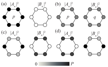
Figure 1: Examples of different modes belonging to family (8)-(10) for the ring with $N=6$. (a) A scalar vortex ($\phi=\varphi=0$) with charge $p$. (b) A symmetric vector vortex ($\phi=\frac{\pi}{4},\varphi=0$) of charge ($p,q$). (c) A discrete necklace ($\phi=\frac{\pi}{4},\varphi=\frac{\pi}{4}$). (d) Another discrete necklace, with $\phi=\frac{\pi}{4},\varphi=-\frac{\pi}{4}$.

In addition to solutions with the explicit ($p=q$) and hidden ($p=-q$) vorticities, for even $N$ there also exist solutions with mixed vorticity, $p=\pm(N/2-q)$. These appear because the constraint (1fg) only needs to be satisfied at a discrete set of points.

3 The linear stability

Linear stability is studied by introducing small perturbations of the form $A_{n}=(U_{n}+a_{n}e^{\lambda z}+b_{n}^{\ast}e^{\lambda^{\ast}z})e^{i\beta_{A}z}$, $B_{n}=(V_{n}+c_{n}e^{\lambda z}+d_{n}^{\ast}e^{\lambda^{\ast}z})e^{i\beta_{B}z}$ and linearizing (1) to derive an eigenvalue problem for $\lambda$. It is convenient to introduce vectors $\mathbf{v}_{n}=(a_{n},b_{n},c_{n},d_{n})$, $\mathbf{E}_{n}=(A_{n},A_{n}^{\ast},B_{n},B_{n}^{\ast})$, writing the eigenvalue problem as

$$(H_{L}+H_{NL})\mathbf{v}_{n}=i\lambda\mathrm{diag}(1,-1,1,-1)\mathbf{v}_{n},$$ (1fk)

where $H_{L}$ is diagonal in the component space (i.e., it does not couple $a_{n}$ to $b_{n}$, etc.), but couples adjacent sites:

$$H_{L}a_{n}=(I-\beta_{A})a_{n}+a_{n-1}+a_{n+1},$$

and similarly for the other components (with $\beta_{A}$ replaced by $\beta_{B}$ for $c_{n},d_{n}$). On the other hand, $H_{NL}$ couples different components, rather than different sites:

$$H_{NL}=\left(\begin{array}[]{cccc}|U_{n}|^{2}&U_{n}^{2}&U_{n}V_{n}^{\ast}&U_{n}V_{n}\\ U_{n}^{\ast 2}&|U_{n}|^{2}&U_{n}^{\ast}V_{n}^{\ast}&U_{n}^{\ast}V_{n}\\ U_{n}^{\ast}V_{n}&U_{n}V_{n}&|V_{n}|^{2}&V_{n}^{2}\\ U_{n}^{\ast}V_{n}^{\ast}&U_{n}V_{n}^{\ast}&V_{n}^{\ast 2}&|V_{n}|^{2}\end{array}\right).$$

This can be compactly written as an outer product, $H_{NL}=\mathbf{E}_{n}\otimes\mathbf{E}_{n}^{\dagger}$.

Equations (1fk) can be solved numerically, as an eigenvalue problem of dimension $4N$. For large $N$, it is relevant to consider some simple limits. For example, when $\varphi=0$ the problem simplifies significantly, the application of the discrete Fourier transform decoupling it into a set of “smaller” eigenvalue problems, each of dimension 4:

$$\left(\begin{array}[]{cc}L_{A}&M\\ M&L_{B}\end{array}\right)\mathbf{v}_{s}=i\lambda\mathbf{v}_{s},$$

where the matrices are defined as

$$L_{A}=\left(\begin{array}[]{cc}P\cos^{2}\phi+\kappa_{p,+}&P\cos^{2}\phi\\ -P\cos^{2}\phi&-P\cos^{2}\phi-\kappa_{p,-}\end{array}\right),$$ (1fn)

$$L_{B}=\left(\begin{array}[]{cc}P\sin^{2}\phi+\kappa_{q,+}&P\sin^{2}\phi\\ -P\sin^{2}\phi&-P\sin^{2}\phi-\kappa_{q,-}\end{array}\right),$$ (1fq)

$$M=\frac{P}{2}\sin 2\phi\left(\begin{array}[]{cc}1&1\\ -1&-1\end{array}\right),$$ (1ft)

with $\kappa_{m,\pm}\equiv 2(\cos\Theta_{m\pm s}-\cos\Theta_{m})$, and $|s|\leq N/2$. In general, the eigenvalues cannot be obtained in an explicit form, but simple expressions are available in some limits. Stability diagrams of family (1fh)-(1fj) in the limit of $\varphi=0$ for $N=6$ are shown in figure 2 for different combinations of topological charges.

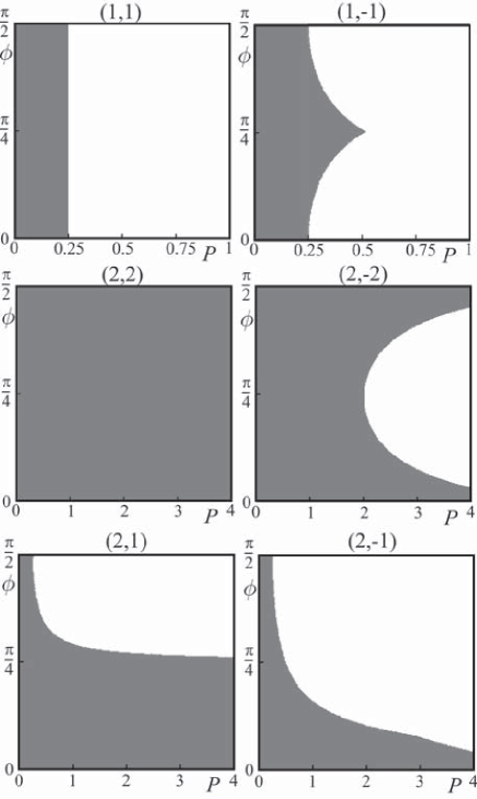
Figure 2: Stable (shaded) and unstable (white) regions in the $(P,\phi)$ parameter plane for composite vortices with different topological charges, indicated in the brackets ($p,q$), in the ring built of $N=6$ sites. Families of hidden-vorticity modes are represented by the top and middle panels in the right column.

When both components have the same charge (which corresponds to the explicit vorticity), the instability threshold is independent of $\phi$, and the stability problem reduces to that for the scalar case: lower charges are unstable, while higher ones are stable [32]. Another situation takes place for the HV states with hidden vorticity: the HV mode (1,-1) encounters instability at a higher power than its scalar counterpart; ultimately, the (1,-1) mode becomes unstable at large powers, in contrast to stable HV solitons in continua [44]. Further, the HV configuration of the (2,-2) type also becomes unstable at large powers, in contrast to its explicit-vorticity (2,2) counterpart, which is completely stable.

Similar stability features are exhibited by the mixed vortex states of the (2,1), (2,-1) types: the state with the greater total charge $p+q$ has a larger stability region. The stability of these solitons depends on the topological charge of the brighter component, i.e., whether the brighter component is stable in the scalar case.

A qualitatively similar behavior is observed for other values of $N$, with the stability dependent on whether the vortex charges are low (smaller than $N/4$) or high (larger than $N/4$). Vortices with the charges equal to $N/4$ represent a special case, as they form a one-parameter family of asymmetric vortex modes, introduced in [55]. This fact complicates the stability analysis, as the stability also depends on the additional parameter.

When $\phi=\pi/4$, an additional pair of zero eigenvalues appears for the hidden- and mixed vortex modes $(p,-p),(p,N/2-p),(p,p-N/2)$, and the linear stability analysis can no longer predict whether the modes are stable. The zero eigenvalues are associated with the degeneracy of family (1fh)-(1fj) with respect to $\varphi$. Calculating the values of the conserved quantities for the family, we obtain $P_{A}=NP\cos^{2}\phi$, $P_{B}=NP\sin^{2}\phi$, $H=2NP(\cos^{2}\phi\cos\Theta_{p}+\sin^{2}\phi\cos\Theta_{q})+NP^{2}/2$ and $S=(1/2)NP\sin\left(2\phi\right)[\cos(\varphi+\gamma)\delta_{p,q}+\sin(\varphi-\gamma)\delta_{p,-q}]$.

We see that for the HV mode with ($p,-p$), when $\phi=\pi/4$, all quantities are independent of the azimuthal modulation $\varphi$, which means that, under small perturbations, the input with $\varphi=0$ can cycle through solutions with different values of $\varphi$, hence we must consider the stability of the family as $\varphi$ is varied. This family can be obtained by applying an isospin rotation to the $\varphi=0$ mode [46]:

$$\left(\begin{array}[]{c}U_{n}\\ V_{n}\end{array}\right)=R_{1}(\varphi)\sqrt{P}\left(\begin{array}[]{c}e^{i\Theta_{p}n}\\ e^{-i\Theta_{p}n}\end{array}\right),$$ (1fu)

which follows from the fact that (1fj) is solved by $\gamma=\varphi$ in this case. This rotation commutes with operator $H_{L}+H_{NL}$ in the linear stability problem, see (1fk). Following the result of [46], the stability is consequently independent of $\varphi$. This result is supported by direct numerical solutions of the linear stability problem. We stress that for other value of $\phi$, the stability does depend on $\varphi$.

Figure 3: The stability of mixed vortex modes as a function of the azimuthal-modulation parameter ($\varphi$) and total power $P$. Shaded: marginal stability. Unshaded: linear instability

The conserved quantities for the mixed vortex modes are independent of $\varphi$ for any value of $\phi$. However, the above reduction of the stability problem to the $\varphi=0$ case is not relevant, as the family cannot be generated by the isospin rotation. Therefore, the stability of the family depends on $\varphi$, as shown in figure 3. The azimuthal modulation lowers the instability threshold for the explicit vortex modes, and it can slightly increase the threshold for the HV mode. In practice, the family will become unstable when $P$ exceeds the lowest instability threshold that occurs as $\varphi$ is varied.

4 Dynamics

The existence of zero eigenvalues in the linear stability problem means that higher-order terms will determine whether the degenerate families are stable. To check the stability, (1) was solved numerically using perturbed initial conditions.

Figure 4 shows the propagation of a perturbed charge-2 HV mode in the waveguide ring built of six sites ($N=6$). The high-frequency oscillations of site powers correspond to frequencies of stable eigenvalues, while the additional low-frequency oscillations correspond to the zero eigenvalue. During this oscillation, the power in each component acquires an azimuthal modulation, however the sum $I_{n}=|A_{n}|^{2}+|B_{n}|^{2}$ remains (on average) constant.

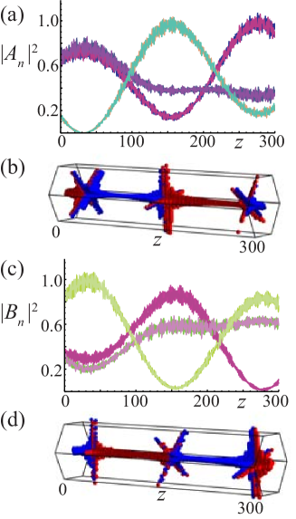
Figure 4: Adiabatic dynamics of the degenerate hidden-vortex family, with parameters $P=1,\phi=\pi/4$, $\varphi=\pi/8$, topological charges (2,-2), and random perturbations added to the initial conditions at the 10% level. (a,c): On-site powers for the two components. (b,d): Vortex lines (red – positive charge, blue – negative charge).

When $z\approx 25$, the amplitudes of the $m=2$ and $m=-2$ Fourier modes are equal and the topological charges of both components vanish [see figure 4(b,d)]. Each component has two pairs of sites with equal powers, and the power vanishes at a pair of sites in one component. The beam profiles at this point resembles those in figure 1(c), which corresponds to a discrete necklace beam with $\varphi=\pi/4$. Increasing $\varphi$ further, the charges of both components flip, and at $z\approx 100$ the azimuthal modulation vanishes, as $\varphi$ attains value $\pi/2$. There is a second charge flip at $z\approx 150$ ($\varphi=3\pi/4$), this time with the other component hosting the pair of vanishing site powers.

Thus we see that the slow oscillations correspond to an adiabatic cycling through the degenerate family of solutions parametrized by $\varphi$. No member of the family is subject to linear instability, therefore the oscillations persist indefinitely long (in excess of $\Delta z=5000$, according to our numerical results).

In contrast to the picture for the HV model outlined above, instability can occur during the adiabatic cycling of the mixed vortex modes, since their stability depends on $\varphi$. This is shown in figure 5, in which the initial condition is the perturbed $\varphi=0$ mode. Initially, it experiences large oscillations in terms of its azimuthal modulation, while preserving its vortex charges and the power sums $I_{n}$. At $z\approx 400$, an unstable value of $\varphi$ is reached and an instability emerges, leading to irregular dynamics in which neither the topological charges nor $I_{n}$ are conserved. If, instead, the $\varphi=\pi/4$ mode is used as the initial condition, this instability sets in immediately.

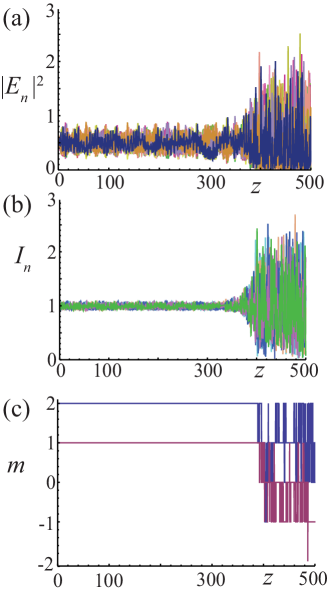
Figure 5: The adiabatic dynamics of the degenerate mixed- vortex family, with $P=1,\phi=\pi/4$, $\varphi=0$, topological charges (2,1) and random perturbations added to the initial conditions at the 5% level. (a) On-site powers of both components. (b) The total power at each site, $I_{n}=|A_{n}|^{2}+|B_{n}|^{2}$. (c) The topological charges.

An additional feature demonstrated by the discrete system is the broken conservation of the OAM. Namely, the two components can exchange their angular momentum with the medium, as well as with each other. We show an example of this in figure 6, in which one component exchanges the angular momentum with the medium, leading to the periodic reversal of its topological charge, while the charge of the other component remains conserved. This type of dynamics is generated by solutions (1fh)-(1fj) with $\phi\neq\pi/4$ and $\varphi$ chosen so as to make the value of $\gamma$ in (1fj) imaginary. The latter acts as a strong azimuthal perturbation, leading to the charge flipping of the second component.

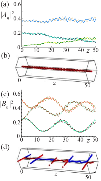
Figure 6: The charge- flipping dynamics of the single component, with $P=1/2,\phi=\pi/5$, $\varphi=\pi/10$, topological charges (2,-1), and random perturbations added to the initial conditions at the 2% level. (a,c): On-site powers for the two components. (b,d): Vortex lines (red – positive charge, blue – negative charge).

5 Conclusions

We have studied the properties of composite vortex modes in circular arrays of nonlinear waveguides. The stability hierarchy of discrete composite vortices can be summarized by stating that the HV (hidden-vorticity) modes suffer instabilities above a critical power, while explicit vortex modes with high topological charges are stable. This hierarchy is opposite to that in continua. Additionally, mixed-vortex modes with different topological charges in the two components exist and can be stable. Degeneracies occur in these families of composite vortex modes, which results in long-lived breather states and persistent vortex-charge flipping.

It should be stressed that the analysis was performed here for the relatively small ring chains, built of $N=6$ sites. For much larger rings, one may expect a change in the stability and dynamics, as, for a fixed diameter of the ring at $N\rightarrow\infty$, the system must go over into the continuum limit, with its reverse picture of the stability domains for the HV and explicit-vorticity modes.

These effects are visible at high powers required for the self-localization in photonic lattices, therefore there is a possibility of observing them in experiments similar to those that were aimed at studying discrete vortices [26, 27] and multivortex solitons [56] in photorefractive crystals. A hexagonal lattice geometry corresponds to the ring built of $6$ sites in our model. We can obtain appropriate experimental parameters for the observation of composite vortices from Ref. [31], which studied double-charge discrete vortex solitons, corresponding to the scalar ($\phi=0$) limit of our nonlinear modes. They used a 20mm long crystal with a bias voltage of 2.2kV/cm, a lattice wave beam with a total power of $75\mu W$ and a $30\mu m$ period. Linear propagation was observed with a probe beam at $532nm$ with a total power of $P\approx 20nW$, while the nonlinear regime was reached at $P\approx 550nW$. With these parameters, the propagation distance is long enough to observe the absence of discrete diffraction at high power (soliton formation) and the modulational instability of unstable modes. To observe composite vortex solitons, all that is required is to split the probe beam into two incoherent components, with the intensity and phase profiles generated using a spatial light modulator. Alternatively, our model can be realized directly in an integrated-optics setting, using a femtosecond-laser written ring of nonlinear waveguides and two incoherent beams [57], although because of the weaker nonlinearity, significantly higher beam powers would be required.

References

References

- [1] Desyatnikov A S, Kivshar Yu S and Torner L 2005 Progress in Optics 47 291
- [2] Nye J F and Berry M V 1974 Proc. R. Soc. London A 336 165
- [3] Soskin M S and Vasnetsov M V 2001 Progress in Optics 42 219
- [4] Malomed B A, Peng G D, Chu P L, Towers I, Buryak A V and Sammut R A 2001 Pramana 57 1061
- [5] Malomed B A, Mihalache D, Wise F and Torner L 2005 J. Optics B: Quant. Semicl. Opt. 7 R53
- [6] Kartashov Y V, Malomed B A and Torner L 2011 Rev. Mod. Phys. 83 247
- [7] Dennis M R, O’Holleran K and Padgett M J 2009 Progress in Optics 52 293
- [8] Gibson G, Courtial J, Padgett M, Vasnetsov M, Pasko V, Barnett S and Franke-Arnold S 2004 Opt. Express 12 5448
- [9] Wang J, Yang J-Y, Fazal I M, Ahmed N, Yan Y, Huang H, Ren Y, Yue Y, Dolinar S, Tur M, Willner A E 2012 Nat. Photonics 6 488
- [10] Firth W J and Skryabin D V 1997 Phys. Rev. Lett. 79 2450
- [11] Torner L and Petrov D V 1997 Electron. Lett. 33 608
- [12] Petrov D V, Torner L, Martorell J, Vilaseca R, Torres J P and Cojocaru C 1998 Opt. Lett. 23 1444
- [13] Quiroga-Teixeiro M and Michinel H 1997 J. Opt. Soc. Am. B 14 2004
- [14] Malomed B A, Crasovan L-C and Mihalache D 2002 Physica D 161 187
- [15] Mihalache D, Mazilu D, Crasovan L-C, Towers I, Malomed B A, Buryak A V, Torner L and Lederer F 2002 Phys. Rev. E 66 016613
- [16] Leblond H, Malomed B A and Mihalache D 2005 Phys. Rev. E 71 036608
- [17] Briedis D, Petersen D, Edmundson D, Królikowski W and Bang O 2005 Opt. Express 13 435443
- [18] Yakimenko A I, Zaliznyak Yu A and Kivshar Yu S 2005 Phys. Rev. E 71 065603
- [19] Mihalache D, Mazilu D, Towers I, Malomed B A and Lederer F 2002 J. Opt. A: Pure Appl. Opt. 4, 615 (2002)
- [20] Borovkova O V, Kartashov Y V, Torner L and Malomed B A 2011 Phys. Rev. E 84 035602(R)
- [21] Kartashov Y V Vysloukh V A and Torner L 2009 Progr. Opt. 52 63
- [22] Christodoulides D N, Lederer F and Silberberg Y 2003 Nature 424 817
- [23] Lederer F, Stegeman G I, Christodoulides D N, Assanto G, Segev M and Silberberg Y 2008 Phys. Reports 463 1
- [24] Malomed B A and Kevrekidis P G 2001 Phys. Rev. E 64 026601
- [25] Pelinovsky D, Kevrekidis P and Frantzeskakis D 2005 Physica D 212 20
- [26] Neshev D N, Alexander T J, Ostrovskaya E A, Kivshar Yu S, Martin H, Makasyuk I and Chen Z 2004 Phys. Rev. Lett. 92 123903
- [27] Fleischer J W, Bartal G, Cohen O, Manela O, Segev M, Hudock J and Christodoulides D N 2004 Phys. Rev. Lett 92 123904
- [28] Sakaguchi H and Malomed B A 2005 Europhys. Lett. 72 698
- [29] Kevrekidis P G, Malomed B A, Chen Z and Frantzeskakis D J 2004 Phys. Rev. E 70 056612
- [30] Law K J H, Song D, Kevrekidis P G, Xu J and Chen Z 2009 Phys Rev A 80 063817
- [31] Terhalle B, Richter T, Law K J H, Göries D, Rose P, Alexander T J, Kevrekidis P G, Desyatnikov A S, Królikowski W, Kaiser F, Denz C and Kivshar Yu S 2009 Phys. Rev A 79 043821
- [32] Desyatnikov A S, Dennis, M R and Ferrando A 2011 Phys. Rev. A 83 063822
- [33] Desyatnikov A S, Neshev D, Ostrovskaya E A, Kivshar Yu S, Królikowski W, Luther-Davies B, Garcia-Ripoll J J and Perez-Garcia V M 2001 Opt. Lett. 26 435
- [34] Desyatnikov A S, Neshev D, Ostrovskaya E A, Kivshar Yu S, McCarthy G, Królikowski W and Luther-Davies B 2002 J. Opt. Soc. Am. B 19 586.
- [35] Desyatnikov A S and Kivshar Yu S 2001 Phys. Rev. Lett. 87 033901
- [36] Bigelow M S, Park Q-H and Boyd R W 2002 Phys. Rev. E 66 046631
- [37] Desyatnikov A S, Kivshar Yu S, Motzek K, Kaiser F, Weilnau C and Denz C 2002 Opt. Lett. 27 634
- [38] Motzek K, Kaiser F, Weilnau C, Denz C, McCarthy G, Królikowski W, Desyatnikov A and Kivshar Yu S 2002 Opt. Commun. 209 501
- [39] Lashkin V M, Ostrovskaya E A, Desyatnikov A S and Kivshar Yu S 2009 Phys. Rev. A 80 013615
- [40] Brtka M, Gammal A and Malomed B A 2010 Phys. Rev. A 82 053610
- [41] Musslimani Z H, Soljačić M, Segev M and Christodoulides D N 2001 Phys. Rev. E 63 066608
- [42] Musslimani Z H, Segev M, Christodoulides D N and Soljačić M 2000 Phys. Rev. Lett. 84 1164
- [43] Desyatnikov A S, Mihalache D, Mazilu D, Malomed B A, Denz C and Lederer F 2005 Phys. Rev. E 71 026615
- [44] Desyatnikov A S, Mihalache D, Mazilu D, Malomed B A and Lederer F 2007 Phys. Lett. A 364 231
- [45] Musslimani Z H, Segev M and Christodoulides D N 2000 Opt. Lett. 25 61
- [46] Desyatnikov A S, Pelinovsky D E and Yang J 2008 J. Math. Sci. 151 3091
- [47] Izdebskaya Y V, Rebling J, Desyatnikov A S and Kivshar Y S 2012 Opt. Lett. 37 767
- [48] Sakaguchi H and Malomed B A 2012 J. Opt. Soc. Am. B 29 2741
- [49] Dong R, Rüter C E, Kip D, Cuevas J, Kevrekidis P G, Song D and Xu J 2011 Phys. Rev. A 83 063816
- [50] Kevrekidis P G, Malomed B A, Frantzeskakis D J and Bishop A R 2003 Phys. Rev. E 67 036614
- [51] Cuevas J, Hoq Q E, Susanto H and Kevrekidis P G 2009 Physica D 238 2216
- [52] Alvarez A, Cuevas J, Romero F R and Kevrekidis P G 2011 Physica D 240 767
- [53] Manakov S V 1973 Zh. Eksp. Teor. Fiz. 65 505
- [54] Ferrando A, Zacarés M, García-March, M-A, Monsoriu J A and de Córdoba P F 2005 Phys. Rev. Lett. 95 123901
- [55] Alexander T J, Sukhorukov A A and Kivshar Yu S 2004 Phys. Rev. Lett. 93 063901
- [56] Terhalle B, Richter T, Desyatnikov A S, Neshev D N, Królikowski W, Kaiser F, Denz C and Kivshar Yu S 2008 Phys. Rev. Lett 101 013903
- [57] Heinrich M, Keil R, Dreisow F, Tünnermann A, Szameit A, Nolte S 2011 App. Phys. B 104 469