Mirror symmetry and the Strominger-Yau-Zaslow conjecture

Abstract.

We trace progress and thinking about the Strominger-Yau-Zaslow conjecture since its introduction in 1996. We begin with the original differential geometric conjecture and its refinements, and explain how insights gained in this context led to the algebro-geometric program developed by the author and Siebert. The objective of this program is to explain mirror symmetry by studying degenerations of Calabi-Yau manifolds. This introduces logarithmic and tropical geometry into the mirror symmetry story, and gives a clear path towards a conceptual understanding of mirror symmetry within an algebro-geometric context. After explaining the overall philosophy, we explain how recent results fit into this program.

Introduction.

Mirror symmetry got its start in 1989 with work of Greene and Plesser [17] and Candelas, Lynker and Schimmrigk [9]. These two works first observed the existence of pairs of Calabi-Yau manifolds exhibiting an exchange of Hodge numbers. Recall that by Yau’s proof of the Calabi conjecture [77], a Calabi-Yau manifold is an $n$-dimensional complex manifold $X$ with a nowhere vanishing holomorphic $n$-form $\Omega$ and a Ricci-flat Kähler metric with Kähler form $\omega$. Ricci-flatness is equivalent to $\omega^{n}=C\Omega\wedge\bar{\Omega}$ for a constant $C$.

The most famous example of a Calabi-Yau manifold is a smooth quintic three-fold $X\subseteq\mathbb{P}^{4}$. The Hodge numbers of $X$ are $h^{1,1}(X)=1$ and $h^{1,2}(X)=101$, with topological Euler characteristic $-200$. The original construction of Greene and Plesser gave a mirror to $X$, as follows. Let $Y\subseteq\mathbb{P}^{4}$ be given by the equation

$$x_{0}^{5}+\cdots+x_{4}^{5}=0,$$

and let

$$G=\{(a_{0},\ldots,a_{4})\in\mathbb{Z}_{5}^{5}\,|\,\sum_{i}a_{i}=0\}.$$

An element $(a_{0},\ldots,a_{4})\in G$ acts on $Y$ by

$$(x_{0},\ldots,x_{4})\mapsto(\xi^{a_{0}}x_{0},\ldots,\xi^{a_{4}}x_{4})$$

for $\xi$ a primitive fifth root of unity. The quotient $Y/G$ is highly singular, but there is a resolution of singularities $\check{X}\rightarrow Y/G$ such that $\check{X}$ is also Calabi-Yau, and one finds $h^{1,1}(\check{X})=101$ and $h^{1,2}(\check{X})=1$, so that $\check{X}$ has topological Euler characteristic $200$.

The relationship between these two Calabi-Yau manifolds proved to be much deeper than just this exchange of Hodge numbers. Pioneering work of Candelas, de la Ossa, Greene and Parkes [10] performed an amazing calculation, following string-theoretic predictions which suggested that certain enumerative calculations on $X$ should give the same answer as certain period calculations on $\check{X}$. The calculations on $\check{X}$, though subtle, could be carried out: these involved integrals of the holomorphic form on $\check{X}$ over three-cycles as the complex structure on $\check{X}$ is varied. On the other hand, the corresponding calculations on $X$ involved numbers of rational curves on $X$ of each degree. For example, the number of lines on a generic quintic threefold is $2875$ and the number of conics is $609250$. String theory thus gave predictions for these numbers for every degree, an astonishing feat given that most of these numbers seemed far beyond the reach of algebraic geometry at the time.

More generally, string theory introduced the concepts of the $A$-model and $B$-model. The $A$-model involves the symplectic geometry of Calabi-Yau manifolds. Properly defined, the counts of rational curves are in fact symplectic invariants, now known as Gromov-Witten invariants. The $B$-model, on the other hand, involves the complex geometry of Calabi-Yau manifolds. Holomorphic forms of course depend on the complex structure, so the period calculations mentioned above can be thought of as $B$-model calculations. Ultimately, string theory predicts an isomorphism between the $A$-model of a Calabi-Yau manifold $X$ and the $B$-model of its mirror, $\check{X}$. The equality of numerical invariants is then a consequence of this isomorphism.

Proofs of these string-theoretic predictions of curve-counting invariants were given by Givental [15] and Lian, Liu and Yau [59], with successively simpler proofs by many other researchers. However, all the proofs relied on the geometry of the ambient space $\mathbb{P}^{4}$ in which the quintic is contained. Roughly speaking, one considers all rational curves in $\mathbb{P}^{4}$, and tries to understand how to compute how many of these are contained in a given quintic hypersurface.

This raised the question: is there some underlying intrinsic geometry to mirror symmetry?

Historically the first approach to an intrinsic formulation of mirror symmetry is Kontsevich’s Homological Mirror Symmetry conjecture, stated in 1994 in [52]. This made mathematically precise the notion of an isomorphism between the $A$- and $B$-models. The homological mirror symmetry conjecture posits an isomorphism between two categories, the Fukaya category of Lagrangian submanifolds of $X$ (the $A$-model) and the derived category of coherent sheaves on the mirror $\check{X}$ (the $B$-model). Morally, this states that the symplectic geometry of $X$ is the same as the complex geometry of $\check{X}$. At the time this conjecture was made, however, there was no clear idea as to how such an isomorphism might be realised, nor did this conjecture state how to construct mirror pairs.

The second approach is due to Strominger, Yau and Zaslow in their 1996 paper [75]. They made a remarkable proposal, based on new ideas in string theory, which gave a very concrete geometric interpretation for mirror symmetry.

Let me summarize, very roughly, the physical argument they used here. Developments in string theory in the mid-1990s introduced the notion of Dirichlet branes, or $D$-branes. These are submanifolds of space-time, with some additional data, which serve as boundary conditions for open strings, i.e., we allow open strings to propagate with their endpoints constrained to lie on a $D$-brane. Remembering that space-time, according to string theory, looks like $\mathbb{R}^{1,3}\times X$, where $\mathbb{R}^{1,3}$ is ordinary space-time and $X$ is a Calabi-Yau three-fold, we can split a $D$-brane into a product of a submanifold of $\mathbb{R}^{1,3}$ and one on $X$. It turned out, simplifying a great deal, that there are two particular types of submanifolds on $X$ of interest: holomorphic $D$-branes, i.e., holomorphic submanifolds with a holomorphic line bundle, and special Lagrangian $D$-branes, which are special Lagrangian submanifolds with flat $U(1)$-bundle:

Definition 0.1.

Let $X$ be an $n$-dimensional Calabi-Yau manifold with $\omega$ the Kähler form of a Ricci-flat metric on $X$ and $\Omega$ a nowhere vanishing holomorphic $n$-form. Then a submanifold $M\subseteq X$ is special Lagrangian if it is Lagrangian, i.e., $\dim_{\mathbb{R}}M=\dim_{\mathbb{C}}X$ and $\omega|_{M}=0$, and in addition, $\operatorname{Im}\Omega|_{M}=0$.

Holomorphic $D$-branes can be viewed as $B$-model objects, and special Lagrangian $D$-branes as $A$-model objects. The isomorphism between the $B$-model on $X$ and the $A$-model on $\check{X}$ then suggests that the moduli space of holomorphic $D$-branes on $X$ should be isomorphic to the moduli space of special Lagrangian $D$-branes on $\check{X}$. (This is now seen as a physical manifestation of the homological mirror symmetry conjecture). Now $X$ itself is the moduli space of points on $X$. So each point on $X$ should correspond to a pair $(M,\nabla)$, where $M\subseteq\check{X}$ is a special Lagrangian submanifold and $\nabla$ is a flat $U(1)$-connection on $M$.

A theorem of McLean [61] tells us that the tangent space to the moduli space of special Lagrangian deformations of a special Lagrangian submanifold $M\subseteq\check{X}$ is $H^{1}(M,\mathbb{R})$. Of course, the moduli space of flat $U(1)$-connections modulo gauge equivalence on $M$ is the torus $H^{1}(M,\mathbb{R})/H^{1}(M,\mathbb{Z})$. In order for this moduli space to be of the correct dimension, we need $\dim H^{1}(M,\mathbb{R})=n$, the complex dimension of $X$. This suggests that $X$ consists of a family of tori which are dual to a family of special Lagrangian tori on $\check{X}$. An elaboration of this argument yields the following conjecture:

Conjecture 0.2.

The Strominger-Yau-Zaslow conjecture. If $X$ and $\check{X}$ are a mirror pair of Calabi-Yau $n$-folds, then there exists fibrations $f:X\rightarrow B$ and $\check{f}:\check{X}\rightarrow B$ whose fibres are special Lagrangian, with general fibre an $n$-torus. Furthermore, these fibrations are dual, in the sense that canonically $X_{b}=H^{1}(\check{X}_{b},\mathbb{R}/\mathbb{Z})$ and $\check{X}_{b}=H^{1}(X_{b},\mathbb{R}/\mathbb{Z})$ whenever $X_{b}$ and $\check{X}_{b}$ are non-singular tori.

This conjecture motivated a great deal of work in the five years following its introduction in 1996, some of which will be summarized in the following sections. There was a certain amount of success, as we shall see, with the conjecture proved for some cases, including the quintic three-fold, at the topological level. Further, the conjecture gave a solid framework for thinking about mirror symmetry at an intuitive level. However, work of Dominic Joyce demonstrated that the conjecture was unlikely to be literally true. Nevertheless, it is possible that weaker limiting forms of the conjecture still hold.

In the first several sections of this survey, I will clarify the conjecture, review what is known about it, and state a weaker form which seems accessible. Most importantly, I will explain how the SYZ conjecture leads to the study of affine manifolds (manifolds with transition functions being affine linear) and hence to an algebro-geometric interpretation of the conjecture, developed by me and Bernd Siebert. This removes the hard analysis, and gives a powerful framework for understanding mirror symmetry at a conceptual level.

The bulk of the paper is devoted to outlining this framework as developed over the last ten years. I explain how affine manifolds are related to degenerations of Calabi-Yau manifolds. Once one begins to consider degenerations, log geometry of K. Kato and Fontaine–Illusie comes into the picture. Conjecturally, the base of the SYZ fibration incorporates key combinatorial information about log structures on degenerations of Calabi-Yau manifolds. Log geometry then gives a connection with tropical geometry and log Gromov-Witten theory, which theoretically allows a description of $A$-model curve counting using tropical geometry. On the mirror side, we explain how again tropical geometry is used to describe complex structures. This identifies tropical geometry as the geometry underlying both sides of mirror symmetry, and guides us towards a conceptual understanding of mirror symmetry. We end with a description of recent work with Pandharipande and Siebert [28] which provides a snapshot of the relationship between the two sides of mirror symmetry.

I would like to thank the organizers of Current Developments in Mathematics 2012 for inviting me to take part in the conference, and Bernd Siebert, my collaborator on much of the work described here. Some of the material appearing in this article was first published in my article “The Strominger-Yau-Zaslow conjecture: From torus fibrations to degenerations,” in Algebraic Geometry: Seattle 2005, edited by D. Abramovich, et al., Proceedings of Symposia in Pure Mathematics Vol. 80, part 1, 149-192, published by the American Mathematical Society. (c) 2009 by the American Mathematical Society. Finally, I would like to thank Lori Lejeune and the Clay Institute for Figure 3.

1. Moduli of special Lagrangian submanifolds

The first step in understanding the SYZ conjecture is to examine the structures which arise on the base of a special Lagrangian fibration. These structures arise from McLean’s theorem on the moduli space of special Lagrangian submanifolds [61], and these structures and their relationships were explained by Hitchin in [42]. We outline some of these ideas here. McLean’s theorem says that the moduli space of deformations of a compact special Lagrangian submanifold of a compact Calabi-Yau manifold $X$ is unobstructed. Further, the tangent space at the point of moduli space corresponding to a special Lagrangian $M\subseteq X$ is canonically isomorphic to the space of harmonic $1$-forms on $M$. This isomorphism is seen explicitly as follows. Let $\nu\in\Gamma(M,N_{M/X})$ be a normal vector field to $M$ in $X$. Then the restriction of the contractions $(\iota(\nu)\omega)|_{M}$ and $(\iota(\nu)\operatorname{Im}\Omega)|_{M}$ are both seen to be well-defined forms on $M$: one needs to lift $\nu$ to a vector field but the choice is irrelevant because $\omega$ and $\operatorname{Im}\Omega$ restrict to zero on $M$. McLean shows that if $M$ is special Lagrangian then

$$\iota(\nu)\operatorname{Im}\Omega=-*\iota(\nu)\omega,$$

where $*$ denotes the Hodge star operator on $M$. Furthermore, $\nu$ corresponds to an infinitesimal deformation preserving the special Lagrangian condition if and only if $d(\iota(\nu)\omega)=d(\iota(\nu)\operatorname{Im}\Omega)=0$. This gives the correspondence between harmonic $1$-forms and infinitesimal special Lagrangian deformations.

Let $f:X\rightarrow B$ be a special Lagrangian fibration with torus fibres, and assume for now that all fibres of $f$ are non-singular. Then we obtain three structures on $B$, namely two affine structures and a metric, as we shall now see.

Definition 1.1.

Let $B$ be an $n$-dimensional manifold. An affine structure on $B$ is given by an atlas $\{(U_{i},\psi_{i})\}$ of coordinate charts $\psi_{i}:U_{i}\rightarrow\mathbb{R}^{n}$, whose transition functions $\psi_{i}\circ\psi_{j}^{-1}$ lie in ${\rm Aff}(\mathbb{R}^{n})$. We say the affine structure is tropical if the transition functions lie in $\mathbb{R}^{n}\rtimes GL(\mathbb{Z}^{n})$, i.e., have integral linear part. We say the affine structure is integral if the transition functions lie in ${\rm Aff}(\mathbb{Z}^{n})$.

If an affine manifold $B$ carries a Riemannian metric $g$, then we say the metric is affine Kähler or Hessian if $g$ is locally given by $g_{ij}=\partial^{2}K/\partial y_{i}\partial y_{j}$ for some convex function $K$ and $y_{1},\ldots,y_{n}$ affine coordinates.

We obtain the three structures as follows:

Affine structure 1. For a normal vector field $\nu$ to a fibre $X_{b}$ of $f$, $(\iota(\nu)\omega)|_{X_{b}}$ is a well-defined $1$-form on $X_{b}$, and we can compute its periods as follows. Let $U\subseteq B$ be a small open set, and suppose we have submanifolds $\gamma_{1},\ldots,\gamma_{n}\subseteq f^{-1}(U)$ which are families of 1-cycles over $U$ and such that $\gamma_{1}\cap X_{b},\ldots,\gamma_{n}\cap X_{b}$ form a basis for $H_{1}(X_{b},\mathbb{Z})$ for each $b\in U$. Consider the $1$-forms $\omega_{1},\ldots,\omega_{n}$ on $U$ defined by fibrewise integration:

$$\omega_{i}(\nu)=\int_{X_{b}\cap\gamma_{i}}\iota(\nu)\omega,$$

for $\nu$ a tangent vector on $B$ at $b$, which we can lift to a normal vector field of $X_{b}$. We have $\omega_{i}=f_{*}(\omega|_{\gamma_{i}})$, and since $\omega$ is closed, so is $\omega_{i}$. Thus there are locally defined functions $y_{1},\ldots,y_{n}$ on $U$ with $dy_{i}=\omega_{i}$. Furthermore, these functions are well-defined up to the choice of basis of $H_{1}(X_{b},\mathbb{Z})$ and constants. Finally, they give well-defined coordinates, as follows from the fact that $\nu\mapsto\iota(\nu)\omega$ yields an isomorphism of $\mathcal{T}_{B,b}$ with $H^{1}(X_{b},\mathbb{R})$ by McLean’s theorem. Thus $y_{1},\ldots,y_{n}$ define local coordinates of a tropical affine structure on $B$.

Affine structure 2. We can play the same trick with $\operatorname{Im}\Omega$: choose submanifolds

$$\Gamma_{1},\ldots,\Gamma_{n}\subseteq f^{-1}(U)$$

which are families of $n-1$-cycles over $U$ and such that $\Gamma_{1}\cap X_{b},\ldots,\Gamma_{n}\cap X_{b}$ form a basis for $H_{n-1}(X_{b},\mathbb{Z})$. We define $\lambda_{i}$ by $\lambda_{i}=-f_{*}(\operatorname{Im}\Omega|_{\Gamma_{i}})$, or equivalently,

$$\lambda_{i}(\nu)=-\int_{X_{b}\cap\Gamma_{i}}\iota(\nu)\operatorname{Im}\Omega.$$

Again $\lambda_{1},\ldots,\lambda_{n}$ are closed $1$-forms, with $\lambda_{i}=d\check{y}_{i}$ locally, and again $\check{y}_{1},\ldots,\check{y}_{n}$ are affine coordinates for a tropical affine structure on $B$.

The McLean metric. The Hodge metric on $H^{1}(X_{b},\mathbb{R})$ is given by

$$g(\alpha,\beta)=\int_{X_{b}}\alpha\wedge*\beta$$

for $\alpha$, $\beta$ harmonic $1$-forms, and hence induces a metric on $B$, which can be written as

$$g(\nu_{1},\nu_{2})=-\int_{X_{b}}\iota(\nu_{1})\omega\wedge\iota(\nu_{2})\operatorname{Im}\Omega.$$

A crucial observation of Hitchin [42] is that these structures are related by the Legendre transform:

Proposition 1.2.

Let $y_{1},\ldots,y_{n}$ be local affine coordinates on $B$ with respect to the affine structure induced by $\omega$. Then locally there is a function $K$ on $B$ such that

$$g(\partial/\partial y_{i},\partial/\partial y_{j})=\partial^{2}K/\partial y_{i}\partial y_{j}.$$

Furthermore, $\check{y}_{i}=\partial K/\partial y_{i}$ form a system of affine coordinates with respect to the affine structure induced by $\operatorname{Im}\Omega$, and if

$$\check{K}(\check{y}_{1},\ldots,\check{y}_{n})=\sum\check{y}_{i}y_{i}-K(y_{1},\ldots,y_{n})$$

is the Legendre transform of $K$, then

$$y_{i}=\partial\check{K}/\partial\check{y}_{i}$$

and

$$\partial^{2}\check{K}/\partial\check{y}_{i}\partial\check{y}_{j}=g(\partial/\partial\check{y}_{i},\partial/\partial\check{y}_{j}).$$

Proof.

Take families $\gamma_{1},\ldots,\gamma_{n},\Gamma_{1},\ldots,\Gamma_{n}$ as above over an open neighbourhood $U$ with the two bases being Poincaré dual, i.e., $(\gamma_{i}\cap X_{b})\cdot(\Gamma_{j}\cap X_{b})=\delta_{ij}$ for $b\in U$. Let $\gamma_{1}^{*},\ldots,\gamma_{n}^{*}$ and $\Gamma_{1}^{*},\ldots,\Gamma_{n}^{*}$ be the dual bases for $\Gamma(U,R^{1}f_{*}\mathbb{Z})$ and $\Gamma(U,R^{n-1}f_{*}\mathbb{Z})$ respectively. From the choice of $\gamma_{i}$’s, we get local coordinates $y_{1},\ldots,y_{n}$ with $dy_{i}=\omega_{i}$, so in particular

$$\delta_{ij}=\omega_{i}(\partial/\partial y_{j})=\int_{\gamma_{i}\cap X_{b}}\iota(\partial/\partial y_{j})\omega,$$

hence $\iota(\partial/\partial y_{j})\omega$ defines the cohomology class $\gamma_{j}^{*}$ in $H^{1}(X_{b},\mathbb{R})$. Similarly, let

$$g_{ij}=-\int_{\Gamma_{i}\cap X_{b}}\iota(\partial/\partial y_{j})\operatorname{Im}\Omega;$$

then $-\iota(\partial/\partial y_{j})\operatorname{Im}\Omega$ defines the cohomology class $\sum_{i}g_{ij}\Gamma_{i}^{*}$ in $H^{n-1}(X_{b},\mathbb{R})$, and $\lambda_{i}=\sum_{j}g_{ij}dy_{j}$. Thus

$$g(\partial/\partial y_{j},\partial/\partial y_{k}) = -\int_{X_{b}}\iota(\partial/\partial y_{j})\omega\wedge\iota(\partial/\partial y_{k})\operatorname{Im}\Omega$$

$$= g_{jk}.$$

On the other hand, let $\check{y}_{1},\ldots,\check{y}_{n}$ be coordinates with $d\check{y}_{i}=\lambda_{i}$. Then

$${\partial\check{y}_{i}/\partial y_{j}}=g_{ij}=g_{ji}={\partial\check{y}_{j}/\partial y_{i}},$$

so $\sum\check{y}_{i}dy_{i}$ is a closed 1-form. Thus there exists locally a function $K$ such that $\partial K/\partial y_{i}=\check{y}_{i}$ and $\partial^{2}K/\partial y_{i}\partial y_{j}=g(\partial/\partial y_{i},\partial/\partial y_{j})$. A simple calculation then confirms that $\partial\check{K}/\partial\check{y}_{i}=y_{i}$. On the other hand,

$$g(\partial/\partial\check{y}_{i},\partial/\partial\check{y}_{j}) = g\left(\sum_{k}{\partial y_{k}\over\partial\check{y}_{i}}{\partial\over\partial y_{k}},\sum_{\ell}{\partial y_{\ell}\over\partial\check{y}_{j}}{\partial\over\partial y_{\ell}}\right)$$

$$= \sum_{k,\ell}{\partial y_{k}\over\partial\check{y}_{i}}{\partial y_{\ell}\over\partial\check{y}_{j}}g(\partial/\partial y_{k},\partial/\partial y_{\ell})$$

$$= \sum_{k,\ell}{\partial y_{k}\over\partial\check{y}_{i}}{\partial y_{\ell}\over\partial\check{y}_{j}}{\partial\check{y}_{k}\over\partial y_{\ell}}$$

$$= {\partial y_{j}\over\partial\check{y}_{i}}={\partial^{2}\check{K}\over\partial\check{y}_{i}\partial\check{y}_{j}}.$$

∎

Thus we introduce the notion of the Legendre transform of an affine manifold with a multi-valued convex function.

Definition 1.3.

Let $B$ be an affine manifold. A multi-valued function $K$ on $B$ is a collection of functions on an open cover $\{(U_{i},K_{i})\}$ such that on $U_{i}\cap U_{j}$, $K_{i}-K_{j}$ is affine linear. We say $K$ is convex if the Hessian $(\partial^{2}K_{i}/\partial y_{j}\partial y_{k})$ is positive definite for all $i$, in any, or equivalently all, affine coordinate systems $y_{1},\ldots,y_{n}$.

Given a pair $(B,K)$ of affine manifold and convex multi-valued function, the Legendre transform of $(B,K)$ is a pair $(\check{B},\check{K})$ where $\check{B}$ is an affine structure on the underlying manifold of $B$ with coordinates given locally by $\check{y}_{i}=\partial K/\partial y_{i}$, and $\check{K}$ is defined by

$$\check{K}_{i}(\check{y}_{1},\ldots,\check{y}_{n})=\sum\check{y}_{j}y_{j}-K_{i}(y_{1},\ldots,y_{n}).$$

Exercise 1.4.

Check that $\check{K}$ is also convex, and that the Legendre transform of $(\check{B},\check{K})$ is $(B,K)$.

Curiously, this Legendre transform between affine manifolds with Hessian metric seems to have first appeared in a work in statistics predating mirror symmetry, see [2].

2. Semi-flat mirror symmetry

Let’s forget about special Lagrangian fibrations for the moment. Instead, we will look at how the structures found on $B$ in the previous section give a toy version of mirror symmetry.

Definition 2.1.

Let $B$ be a tropical affine manifold.

1. Denote by $\Lambda\subseteq\mathcal{T}_{B}$ the local system of lattices generated locally by $\partial/\partial y_{1},\ldots,\partial/\partial y_{n}$, where $y_{1},\ldots,y_{n}$ are local affine coordinates. This is well-defined because transition maps are in $\mathbb{R}^{n}\rtimes GL_{n}(\mathbb{Z})$. Set

   $$X(B):=\mathcal{T}_{B}/\Lambda.$$

   This is a torus bundle over $B$. In addition, $X(B)$ carries a complex structure defined locally as follows. Let $U\subseteq B$ be an open set with affine coordinates $y_{1},\ldots,y_{n}$, so $\mathcal{T}_{U}$ has coordinate functions $y_{1},\ldots,y_{n}$, $x_{1}=dy_{1},\ldots,x_{n}=dy_{n}$. Then

   $$q_{j}=e^{2\pi i(x_{j}+iy_{j})}$$

   gives a system of holomorphic coordinates on $T_{U}/\Lambda|_{U}$, and the induced complex structure is independent of the choice of affine coordinates. This is called the semi-flat complex structure on $X(B)$.

   Later we will need a variant of this: for $\epsilon>0$, set

   $$X_{\epsilon}(B):=\mathcal{T}_{B}/\epsilon\Lambda.$$

   This has a complex structure with coordinates given by

   $$q_{j}=e^{2\pi i(x_{j}+iy_{j})/\epsilon}.$$

   (As we shall see later, the limit $\epsilon\rightarrow 0$ corresponds to a “large complex structure limit.”)

2. Define $\check{\Lambda}\subseteq\mathcal{T}^{*}_{B}$ to be the local system of lattices generated locally by $dy_{1},\ldots,dy_{n}$, with $y_{1},\ldots,y_{n}$ local affine coordinates. Set

   $$\check{X}(B):=\mathcal{T}^{*}_{B}/\check{\Lambda}.$$

   Of course $\mathcal{T}^{*}_{B}$ carries a canonical symplectic structure, and this symplectic structure descends to $\check{X}(B)$.

∎

We write $f:X(B)\rightarrow B$ and $\check{f}:\check{X}(B)\rightarrow B$ for these torus fibrations; these are clearly dual.

Now suppose in addition we have a Hessian metric $g$ on $B$, with local potential function $K$. Then the following propositions show that in fact both $X(B)$ and $\check{X}(B)$ become Kähler manifolds.

Proposition 2.2.

$K\circ f$ is a (local) Kähler potential on $X(B)$, defining a Kähler form $\omega=2i\partial\bar{\partial}(K\circ f)$. This metric is Ricci-flat if and only if $K$ satisfies the real Monge-Ampère equation

$$\det{\partial^{2}K\over\partial y_{i}\partial y_{j}}=constant.$$

Proof.

Working locally with affine coordinates $(y_{j})$ and complex coordinates

$$z_{j}={1\over 2\pi i}\log q_{j}=x_{j}+iy_{j},$$

we compute $\omega=2i\partial\bar{\partial}(K\circ f)={i\over 2}\sum{\partial^{2}K\over\partial y_{j}\partial y_{k}}dz_{j}\wedge d\bar{z}_{k}$ which is clearly positive. Furthermore, if $\Omega=dz_{1}\wedge\cdots\wedge dz_{n}$, then $\omega^{n}$ is proportional to $\Omega\wedge\bar{\Omega}$ if and only if $\det(\partial^{2}K/\partial y_{j}\partial y_{k})$ is constant. ∎

We write this Kähler manifold as $X(B,K)$.

Dually we have

Proposition 2.3.

In local canonical coordinates $y_{i},\check{x}_{i}$ on $\mathcal{T}^{*}_{B}$, the complex coordinate functions $z_{j}=\check{x}_{j}+i\partial K/\partial y_{j}$ on $\mathcal{T}^{*}_{B}$ induce a well-defined complex structure on $\check{X}(B)$, with respect to which the canonical symplectic form $\omega$ is the Kähler form of a metric. Furthermore this metric is Ricci-flat if and only if $K$ satisfies the real Monge-Ampère equation

$$\det{\partial^{2}K\over\partial y_{j}\partial y_{k}}=constant.$$

Proof.

It is easy to see that an affine linear change in the coordinates $y_{j}$ (and hence an appropriate change in the coordinates $\check{x}_{j}$) results in a linear change of the coordinates $z_{j}$, so they induce a well-defined complex structure invariant under $\check{x}_{j}\mapsto\check{x}_{j}+1$, and hence a complex structure on $\check{X}(B)$. Then one computes that

$$\omega=\sum d\check{x}_{j}\wedge dy_{j}={i\over 2}\sum g^{jk}dz_{j}\wedge d\bar{z}_{k}$$

where $g_{ij}=\partial^{2}K/\partial y_{j}\partial y_{k}$. Then the metric is Ricci-flat if and only if $\det(g^{jk})=constant$, if and only if $\det(g_{jk})=constant$. ∎

As before, we call this Kähler manifold $\check{X}(B,K)$.

This motivates the definition

Definition 2.4.

An affine manifold with metric of Hessian form is a Monge-Ampère manifold if the local potential function $K$ satisfies the Monge-Ampère equation $\det(\partial^{2}K/\partial y_{i}\partial y_{j})=constant$.

Hessian and Monge-Ampère manifolds were first studied by Cheng and Yau in [12].

Exercise 2.5.

Show that the identification of $\mathcal{T}_{B}$ and $\mathcal{T}^{*}_{B}$ given by a Hessian metric induces a canonical isomorphism $X(B,K)\cong\check{X}(\check{B},\check{K})$ of Kähler manifolds, where $(\check{B},\check{K})$ is the Legendre transform of $(B,K)$.

There is a key extra parameter which appears in mirror symmetry known as the $B$-field. This appears as a field in the non-linear sigma model with Calabi-Yau target space, and is required mathematically to make sense of mirror symmetry. Mirror symmetry roughly posits an isomorphism between the complex moduli space of a Calabi-Yau manifold $X$ and the Kähler moduli space of $\check{X}$. If one interprets the Kähler moduli space to mean the space of all Ricci-flat Kähler forms on $\check{X}$, then one obtains only a real manifold as moduli space, and one needs a complex manifold to match up with the complex moduli space of $X$. The $B$-field is interpreted as an element ${\bf B}\in H^{2}(\check{X},\mathbb{R}/\mathbb{Z})$, and one views ${\bf B}+i\omega$ as a complexified Kähler class on $\check{X}$ for $\omega$ a Kähler class on $\check{X}$.

In the context of our toy version of mirror symmetry, we view the $B$-field as an element ${\bf B}\in H^{1}(B,\Lambda_{\mathbb{R}}/\Lambda)$, where $\Lambda_{\mathbb{R}}=\Lambda\otimes_{\mathbb{Z}}\mathbb{R}$. This does not quite agree with the above definition of the $B$-field, as this group does not necessarily coincide with $H^{2}(\check{X},\mathbb{R}/\mathbb{Z})$. However, in many important cases, such as for simply connected Calabi-Yau threefolds with torsion-free integral cohomology, these two groups do coincide. More generally, including the case of K3 surfaces and abelian varieties, one would need to pass to generalized complex structures [43], [39], [7], [3], [44], which we do not wish to do here.

Noting that a section of $\Lambda_{\mathbb{R}}/\Lambda$ over an open set $U$ can be viewed as a section of $\mathcal{T}_{U}/\Lambda|_{U}$, such a section acts on $\mathcal{T}_{U}/\Lambda|_{U}$ via translation, and this action is in fact holomorphic with respect to the semi-flat complex structure. Thus a Čech 1-cocycle $(U_{ij},\beta_{ij})$ representing ${\bf B}$ allows us to reglue $X(B)$ via translations over the intersections $U_{ij}$. This is done by identifying the open subsets $f^{-1}(U_{ij})\subseteq f^{-1}(U_{i})$ and $f^{-1}(U_{ij})\subseteq f^{-1}(U_{j})$ via the automorphism of $f^{-1}(U_{ij})$ given by translation by the section $\beta_{ij}$. This gives a new complex manifold $X(B,{\bf B})$. If in addition there is a multi-valued potential function $K$ defining a metric, these translations preserve the metric and yield a Kähler manifold $X(B,{\bf B},K)$.

Thus the full toy version of mirror symmetry is as follows:

Construction 2.6 (The toy mirror symmetry construction).

Suppose given an affine manifold $B$ with potential $K$ and $B$-fields ${\bf B}\in H^{1}(B,\Lambda_{\mathbb{R}}/\Lambda)$, $\check{\bf B}\in H^{1}(B,\check{\Lambda}_{\mathbb{R}}/\check{\Lambda})$. It is not difficult to see, and you will have seen this already if you’ve done Exercise 2.5, that the local system $\check{\Lambda}$ defined using the affine structure on $B$ is the same as the local system $\Lambda$ defined using the affine stucture on $\check{B}$. So we say the pair

$$(X(B,{\bf B},K),\check{\bf B})$$

is mirror to

$$(X(\check{B},\check{\bf B},\check{K}),\bf B).$$

This provides a reasonably fulfilling picture of mirror symmetry in a simple context. Many more aspects of mirror symmetry can be worked out in this semi-flat context, see [55] and [3], Chapter 6. This semi-flat case is an ideal testing ground for concepts in mirror symmetry. However, ultimately this only sheds limited insight into the general case. The only compact Calabi-Yau manifolds with semi-flat Ricci-flat metric which arise in this way are complex tori (shown by Cheng and Yau in [12]). To deal with more interesting cases, we need to allow singular fibres, and hence, singularities in the affine structure of $B$. The existence of singular fibres are fundamental for the most interesting aspects of mirror symmetry.

3. Affine manifolds with singularities

To deal with singular fibres, we define

Definition 3.1.

A (tropical, integral) affine manifold with singularities is a $(C^{0})$ manifold $B$ with an open subset $B_{0}\subseteq B$ which carries a (tropical, integral) affine structure, and such that $\Gamma:=B\setminus B_{0}$ is a locally finite union of locally closed submanifolds of codimension $\geq 2$.

Here we will give a relatively simple construction of such affine manifolds with singularities; a broader class of examples is given in [22]; see also [40] and [41].

Let $\Delta$ be a reflexive polytope in $M_{\mathbb{R}}=M\otimes_{\mathbb{Z}}\mathbb{R}$, where $M=\mathbb{Z}^{n}$. This means that $\Delta$ is a lattice polytope with a unique interior integral point $0\in\Delta$, and the polar dual polytope

$$\nabla:=\{n\in N_{\mathbb{R}}|\hbox{$\langle m,n\rangle\geq-1$ for all $m\in\Delta$}\}$$

is also a lattice polytope.

Let $B=\partial\Delta$, and let $\mathscr{P}$ be a decomposition of $B$ into lattice polytopes, i.e., $\mathscr{P}$ is a set of lattice polytopes contained in $B$ such that (1) $B=\bigcup_{\sigma\in\mathscr{P}}\sigma$; (2) $\sigma_{1},\sigma_{2}\in\mathscr{P}$ implies $\sigma_{1}\cap\sigma_{2}$ lies in $\mathscr{P}$ and is a face of both $\sigma_{1}$ and $\sigma_{2}$; (3) if $\sigma\in\mathscr{P}$, any face of $\sigma$ lies in $\mathscr{P}$.

We now define a structure of integral affine manifold with singularities on $B$, with discriminant locus $\Gamma\subseteq B$ defined as follows. Let $\operatorname{Bar}(\mathscr{P})$ denote the first barycentric subdivision of $\mathscr{P}$ and let $\Gamma\subseteq B$ be the union of all simplices of $\operatorname{Bar}(\mathscr{P})$ not containing a vertex of $\mathscr{P}$ (a zero-dimensional cell) or intersecting the interior of a maximal cell of $\mathscr{P}$. Setting $B_{0}:=B\setminus\Gamma$, we define an affine structure on $B_{0}$ as follows. $B_{0}$ has an open cover

$$\{W_{\sigma}|\hbox{$\sigma\in\mathscr{P}$ maximal}\}\cup\{W_{v}|\hbox{$v\in\mathscr{P}$ a vertex}\}$$

where $W_{\sigma}=\operatorname{Int}(\sigma)$, the interior of $\sigma$, and

$$W_{v}=\bigcup_{\tau\in\operatorname{Bar}(\mathscr{P})\atop v\in\tau}\operatorname{Int}(\tau)$$

is the (open) star of $v$ in $\operatorname{Bar}(\mathscr{P})$. We define an affine chart

$$\psi_{\sigma}:W_{\sigma}\hookrightarrow\mathbb{A}_{\sigma}\subseteq N_{\mathbb{R}}$$

given by the inclusion of $W_{\sigma}$ in $\mathbb{A}_{\sigma}$, which denotes the unique $(n-1)$-dimensional affine hyperplane in $N_{\mathbb{R}}$ containing $\sigma$. Also, take $\psi_{v}:W_{v}\rightarrow M_{\mathbb{R}}/\mathbb{R}v$ to be the projection. One checks easily that for $v\in\sigma$, $\psi_{\sigma}\circ\psi_{v}^{-1}$ is integral affine linear (integrality follows from reflexivity of $\Delta$!) so $B$ is an integral affine manifold with singularities.

Example 3.2.

Let $\Delta\subseteq\mathbb{R}^{4}$ be the convex hull of the points

$$(-1,-1,-1,-1),$$

$$(4,-1,-1,-1),$$

$$(-1,4,-1,-1),$$

$$(-1,-1,4,-1),$$

$$(-1,-1,-1,4).$$

Choose a triangulation $\mathscr{P}$ of $B=\partial\Delta$ into standard simplices; this can be done in a regular way so that the restriction of $\mathscr{P}$ to each two-dimensional face of $\Delta$ is as given by the light lines in Figure 1. This gives a discriminant locus $\Gamma$ depicted by the dark lines in the figure; the line segments coming out of the boundary of the two-face are meant to illustrate the pieces of discriminant locus contained in adjacent two-faces. The discriminant locus there is not contained in the plane of the two-face. In particular, the discriminant locus is not planar at the vertices of $\Gamma$ on the edges of $\Xi$ with respect to the affine structure we define. Note $\Gamma$ is a trivalent graph, with two types of trivalent vertices, the non-planar ones just mentioned and the planar vertices contained in the interior of two-faces.

Figure 1.

For an affine manifold, the monodromy of the local system $\Lambda$ is an important feature of the affine structure. In this example, it is very useful to analyze this monodromy around loops about the discriminant locus. If $v$ is a vertex of $\Gamma$ contained in the interior of a two-face of $\Delta$, one can consider loops based near $v$ in $B_{0}$ around the three line segments of $\Gamma$ adjacent to $v$. It is an enjoyable exercise to calculate that these monodromy matrices take the form, in a suitable basis,

$$T_{1}=\begin{pmatrix}1&0&0\\ 1&1&0\\ 0&0&1\end{pmatrix},T_{2}=\begin{pmatrix}1&0&0\\ 0&1&0\\ 1&0&1\end{pmatrix},T_{3}=\begin{pmatrix}1&0&0\\ -1&1&0\\ -1&0&1\end{pmatrix}.$$

They are computed by studying the composition of transition maps between charts that a loop passes through. These matrices can be viewed as specifying the obstruction to extending the affine structure across a neighbourhood of $v$ in $\Gamma$. Of course, the monodromy of $\check{\Lambda}$ is the transpose inverse of these matrices. Similarly, if $v$ is a vertex of $\Gamma$ contained in an edge of $\Delta$, then the monodromy will take the form

$$T_{1}=\begin{pmatrix}1&-1&0\\ 0&1&0\\ 0&0&1\end{pmatrix},T_{2}=\begin{pmatrix}1&0&-1\\ 0&1&0\\ 0&0&1\end{pmatrix},T_{3}=\begin{pmatrix}1&1&1\\ 0&1&0\\ 0&0&1\end{pmatrix}.$$

So we see that the monodromy of the two types of vertices are interchanged between $\Lambda$ and $\check{\Lambda}$.

One main result of [20] is

Theorem 3.3.

If $B$ is a three-dimensional tropical affine manifold with singularities such that $\Gamma$ is trivalent and the monodromy of $\Lambda$ at each vertex is one of the above two types, then $f_{0}:X(B_{0})\rightarrow B_{0}$ can be compactified to a topological fibration $f:X(B)\rightarrow B$. Dually, $\check{f}_{0}:\check{X}(B_{0})\rightarrow B_{0}$ can be compactified to a topological fibration $\check{f}:\check{X}(B)\rightarrow B$. Both $X(B)$ and $\check{X}(B)$ are topological manifolds.

We won’t give any details here of how this is carried out, but it is not particularly difficult, as long as one restricts to the category of topological (not $C^{\infty}$) manifolds. However, it is interesting to look at the singular fibres we need to add.

If $b\in\Gamma$ is a point which is not a vertex of $\Gamma$, then $f^{-1}(b)$ is homeomorphic to $I_{1}\times S^{1}$, where $I_{1}$ denotes a Kodaira type $I_{1}$ elliptic curve, i.e., a pinched torus.

If $v$ is a vertex of $\Gamma$, with monodromy of the first type, then $f^{-1}(v)=S^{1}\times S^{1}\times S^{1}/\sim$, with $(a,b,c)\sim(a^{\prime},b^{\prime},c^{\prime})$ if $(a,b,c)=(a^{\prime},b^{\prime},c^{\prime})$ or $a=a^{\prime}=1$, where $S^{1}$ is identified with the unit circle in $\mathbb{C}$. This is the three-dimensional analogue of a pinched torus, and $\chi(f^{-1}(v))=+1$. We call this a positive fibre.

If $v$ is a vertex of $\Gamma$, with monodromy of the second type, then $f^{-1}(v)$ can be described as $S^{1}\times S^{1}\times S^{1}/\sim$, with $(a,b,c)\sim(a^{\prime},b^{\prime},c^{\prime})$ if $(a,b,c)=(a^{\prime},b^{\prime},c^{\prime})$ or $a=a^{\prime}=1$, $b=b^{\prime}$, or $a=a^{\prime},b=b^{\prime}=1$. The singular locus of this fibre is a figure eight, and $\chi(f^{-1}(v))=-1$. We call this a negative fibre.

So we see a very concrete local consequence of SYZ duality: in the compactifications $X(B)$ and $\check{X}(B)$, the positive and negative fibres are interchanged. Of course, this results in the observation that the Euler characteristic changes sign under mirror symmetry for Calabi-Yau threefolds.

Example 3.4.

Continuing with Example 3.2, it was proved in [20] that $\check{X}(B)$ is homeomorphic to the quintic and $X(B)$ is homeomorphic to the mirror quintic. Modulo a paper [30] whose appearance has been long-delayed because of other, more pressing, projects, the results of [22] imply that the SYZ conjecture holds for all complete intersections in toric varieties at a topological level.

W.-D. Ruan in [70] gave a description of Lagrangian torus fibrations for hypersurfaces in toric varieties using a symplectic flow argument, and his construction should coincide with a symplectic compactification of the symplectic manifolds $\check{X}(B_{0})$. In the three-dimensional case, such a symplectic compactification has been constructed by Ricardo Castaño-Bernard and Diego Matessi [8]. If this compactification is applied to the affine manifolds with singularities described here, the resulting symplectic manifolds should be symplectomorphic to the corresponding toric hypersurface, but this has not yet been shown.

4. Tropical geometry

Recalling that mirror symmetry is supposed to allow us to count curves, let us discuss at an intuitive level how the picture so far gives us insight into this question. Let $B$ be a tropical affine manifold. Then as we saw, $X(B)$ carries the semi-flat complex structure, and it is easy to describe some complex submanifolds of $X(B)$ as follows. Let $L\subseteq B$ be a linear subspace with rational slope, i.e., the tangent space $\mathcal{T}_{L,b}$ to $L$ at any $b\in L$ can be written as $M\otimes_{\mathbb{Z}}\mathbb{R}$ for some sublattice $M\subseteq\Lambda_{b}$. Then we obtain a submanifold

$$X(L):=\mathcal{T}_{L}/(\mathcal{T}_{L}\cap\Lambda)\subseteq X(B).$$

One checks easily that this is a complex submanifold. For example, if $B=\mathbb{R}^{n}$, so that $X(B)$ is just an algebraic torus $(\mathbb{C}^{*})^{n}$ with coordinates $q_{1},\ldots,q_{n}$, and $L\subseteq B$ is a codimension $p$ affine linear subspace defined by equations

$$\sum_{j}c_{ij}y_{j}=d_{i},\quad 1\leq i\leq p,$$

with $c_{ij}\in\mathbb{Z}$, $d_{i}\in\mathbb{R}$, then the corresponding submanifold of $X(B)$ is the subtorus given by the equations

$$\prod_{j}q_{j}^{c_{ij}}=e^{-2\pi d_{j}},\quad 1\leq i\leq p.$$

Of course, subtori of tori are not particularly interesting. How might we build more complicated submanifolds? Let us focus on curves, where we take the linear submanifolds of $B$ to be of dimension one. Then if we take $L$ to be a line segment, ray, or line, $X(L)$ is a cylinder, with or without boundary in the various cases. We can then try to glue such cylinders together to obtain more complicated curves. For example, imagine we are given rays meeting at a point $b\in B=\mathbb{R}^{2}$ as pictured in Figure 2. Take primitive integral tangent vectors $v_{1},v_{2},v_{3}\in\mathbb{R}^{2}$ to $L_{1},L_{2}$ and $L_{3}$ pointing outwards from the point $b$ where the three segments intersect. Now we have the three cylinders $X(L_{i})$ which do not match up over $b$: the fibre $f^{-1}(b)=\mathbb{R}^{2}/\mathbb{Z}^{2}$ intersects $X(L_{i})$ in a circle $\mathbb{R}v_{i}/\mathbb{Z}v_{i}$. These circles are represented in $H_{1}(f^{-1}(b),\mathbb{Z})=\Lambda_{b}$ precisely by the vectors $v_{1},v_{2},v_{3}$, and so the condition that the circles bound a surface in $f^{-1}(b)$ is that $v_{1}+v_{2}+v_{3}=0$. Thus, if this condition holds, we can glue in a surface $S$ contained in $f^{-1}(b)$ so that $X(L_{1})\cup X(L_{2})\cup X(L_{3})\cup S$ now has no boundary at $b$. Of course, it is very far from being a holomorphic submanifold. The expectation, however, is that this sort of object can be deformed to a nearby holomorphic curve.

Figure 2.

Precisely, continuing with the above example, suppose $b=0$ and $v_{1}=(1,0)$, $v_{2}=(0,1)$ and $v_{3}=(-1,-1)$. With holomorphic coordinates $q_{1},q_{2}$ on $X(B)=(\mathbb{C}^{*})^{2}$, consider the curve $C\subseteq(\mathbb{C}^{*})^{2}$ defined by $1+q_{1}+q_{2}=0$. Look at the image of this curve under the map $f:X(B)\rightarrow B$, which here can be written explicitly as $(q_{1},q_{2})\mapsto{-1\over 2\pi}(\log|q_{1}|,\log|q_{2}|)$. One finds that one obtains a thickening of the trivalent graph above, typically known as an amoeba. Further, if one considers not $X(B)$ but $X_{\epsilon}(B)$, where now holomorphic coordinates are given by $q_{j}=e^{2\pi i(x_{j}+iy_{j})/\epsilon}$ and $f_{\epsilon}:X_{\epsilon}(B)\rightarrow B$ is given by $(q_{1},q_{2})\mapsto-{\epsilon\over 2\pi}(\log|q_{1}|,\log|q_{2}|)$, one finds that as $\epsilon\rightarrow 0$, $f_{\epsilon}(C)$ converges to the trivalent graph in the above figure. In this sense the trivalent graph on $B$ is a limiting version of curves on a family of varieties tending towards a large complex structure limit.

This basic picture for curves in algebraic tori is now very well studied. In particular, this study spawned the subject of tropical geometry. The word tropical is motivated by the role that the tropical semiring plays. This is the semiring $(\mathbb{R},\oplus,\odot)$ where addition and multiplication are given by

$$a\oplus b:={} \min(a,b)$$

$$a\odot b:={} a+b.$$

The word “tropical” is used in honor of the Brazilian mathematician Imre Simon, who pioneered use of this semi-ring.

We now consider polynomials over the tropical semiring, as follows. Let $S\subseteq\mathbb{Z}^{n}$ be a finite subset, and consider tropical polynomials on $\mathbb{R}^{n}$ of the form

$$g:=\sum_{(p_{1},\ldots,p_{n})\in S}c_{p_{1}\ldots p_{n}}x_{1}^{p_{1}}\cdots x_{n}^{p_{n}}$$

where the coefficients lie in $\mathbb{R}$ and the operations are in the tropical semiring. Then $g$ is a convex piecewise linear function on $\mathbb{R}^{n}$, and the locus where $g$ is not linear is called a tropical hypersurface. In particular, in the case $n=2$, we obtain a tropical curve. In the example of Figure 2, the relevant tropical polynomial could be taken to be $0\oplus x_{1}\oplus x_{2}$.

While the tropical semiring has been used extensively in tropical geometry, it is not so convenient for us to view our tropical curves on $B$ as being defined by equations, since typically these curves will be of high codimension. Instead, it is better to follow Mikhalkin [62] and use parameterized tropical curves.

The domain of a parameterized tropical curve will be a weighted graph. In what follows, $\overline{\Gamma}$ will denote a connected graph. Such a graph can be viewed in two different ways. First, it can be viewed as a purely combinatorial object, i.e., a set $\overline{\Gamma}^{[0]}$ of vertices and a set $\overline{\Gamma}^{[1]}$ of edges consisting of unordered pairs of elements of $\overline{\Gamma}^{[0]}$, indicating the endpoints of an edge. We can also view $\overline{\Gamma}$ as the topological realization of the graph, i.e., a topological space which is the union of line segments corresponding to the edges. We shall confuse these two viewpoints at will. We will then denote by $\Gamma$ the topological space obtained from $\overline{\Gamma}$ by deleting the univalent vertices of $\overline{\Gamma}$, so that $\Gamma$ may have some non-compact edges.

We also take $\overline{\Gamma}$ to come with a weight function, a map

$$w:\overline{\Gamma}^{[1]}\rightarrow\mathbb{N}=\{0,1,2,\ldots\}.$$

Replacing $\mathbb{R}^{n}$ with a general tropical affine manifold $B$, we now arrive at the following definition:

Definition 4.1.

A parameterized tropical curve in $B$ is a continuous map

$$h:\Gamma\rightarrow B$$

where $\Gamma$ is obtained from a graph $\overline{\Gamma}$ as above, satisfying the following two properties:

1. If $E\in\Gamma^{[1]}$ and $w(E)=0$, then $h|_{E}$ is constant; otherwise $h|_{E}$ is a proper embedding of $E$ into $B$ as a line segment, ray or line of rational slope.

2. The balancing condition. Let $V\in\overline{\Gamma}^{[0]}$ be a vertex with valency larger than $1$, with adjacent edges $E_{1},\ldots,E_{\ell}$. Let $v_{i}\in\Lambda_{h(V)}$ be a primitive tangent vector to $h(E_{i})$ at $h(V)$, pointing away from $h(V)$. Then

   $$\sum_{i=1}^{\ell}w(E_{i})v_{i}=0.$$

Here the balancing condition is just expressing the topological requirement that the boundaries of the various cylinders $X(h(E_{i}))\subseteq X(B)$ can be connected up with a surface contained in the fibre of $X(B)\rightarrow B$ over $h(V)$. The weights can be interpreted as taking the cylinders $X(h(E_{i}))$ with multiplicity.

An important question then arises:

Question 4.2.

When can a given parameterized tropical curve be viewed as a limit of holomorphic curves in $X_{\epsilon}(B)$ as $\epsilon\rightarrow 0$?

This question has attracted a great deal of attention when $B=\mathbb{R}^{n}$, with completely satisfactory results in the case $n=2$ (Answer: always), and less complete results when $n\geq 3$. The $n=2$ case was first treated by Mikhalkin [62], and resuts in all dimensions were first obtained by Nishinou and Siebert [64]. In particular, Mikhalkin proved that in this two-dimensional case, one can calculate numbers of curves of a given degree and genus passing through a fixed set of points, showing that difficult holomorphic enumerative problems can be solved by a purely combinatorial approach. This work gives hope that one can really count curves combinatorially in much more general settings. In the two-dimensional case, again, my own work [24] showed that the mirror side (for mirror symmetry for $\mathbb{P}^{2}$) could also be interpreted tropically, giving a completely tropical interpretation of mirror symmetry for $\mathbb{P}^{2}$.

So far we have not considered the case that $B$ has singularities. In case $B$ has singularities, we expect that one should be able to relax the balancing condition when a vertex falls inside of a point of the singular locus, and in particular one can allow univalent vertices which map to the singular locus. The reason for this is that once we compactify $X(B_{0})$ to $X(B)$, one expects to find holomorphic disks fibering over line segments emanating from singular points: see Figure 3 for a depiction of this when $B$ is two-dimensional, having isolated singularities.

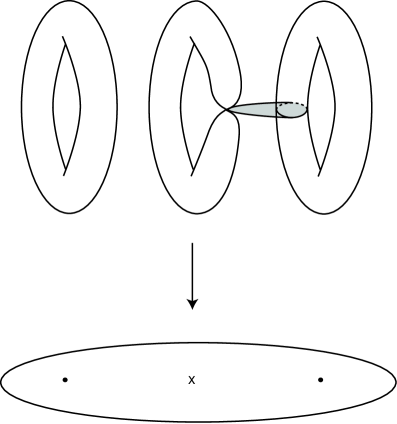
Figure 3.

We will avoid giving a precise definition of what a tropical curve should mean in the case that $B$ has singularities, largely because it is not clear yet what the precise definition should be. Hopefully, though, this discussion makes it clear that at an intuitive level, counting curves should be something which can be done on $B$.

5. The problems with the SYZ conjecture, and how to get around them

The discussion of §3 demonstrates that the SYZ conjecture gives a beautiful description of mirror symmetry at a purely topological level. This, by itself, can often be useful, but fails to get at the original hard differential geometric conjecture and fails to give insight into why mirror symmetry counts curves.

In order for the full-strength version of the SYZ conjecture to hold, the strong version of duality for topological torus fibrations we saw in §3 should continue to hold at the special Lagrangian level. This would mean that a mirror pair $X,\check{X}$ would possess special Lagrangian torus fibrations $f:X\rightarrow B$ and $\check{f}:\check{X}\rightarrow B$ with codimension two discriminant loci, and the discriminant loci of $f$ and $\check{f}$ would coincide. These fibrations would then be dual away from the discriminant locus.

There are examples of special Lagrangian fibrations on non-compact toric varieties $X$ with discriminant locus looking very similar to what we have described in the topological case. In particular, if $X$ is an $n$-dimensional Ricci-flat Kähler manifold with a $T^{n-1}$-action preserving the metric and holomorphic $n$-form, then $X$ will have a very nice special Lagrangian fibration with codimension two discriminant locus. (See [21] and [16]). However, Dominic Joyce (see [48] and other papers cited therein) began studying some three-dimensional $S^{1}$-invariant examples, and discovered quite different behaviour. There is an argument in [19] that if a special Lagrangian fibration is $C^{\infty}$, then the discriminant locus will be (Hausdorff) codimension two. However, Joyce discovered examples which were not differentiable, but only piecewise differentiable, and furthermore, had a codimension one discriminant locus:

Example 5.1.

Define $F:\mathbb{C}^{3}\rightarrow\mathbb{R}\times\mathbb{C}$ by $F(z_{1},z_{2},z_{3})=(a,c)$ with $2a=|z_{1}|^{2}-|z_{2}|^{2}$ and

$$c=\begin{cases}z_{3}&a=z_{1}=z_{2}=0\\ z_{3}-\bar{z}_{1}\bar{z}_{2}/|z_{1}|&a\geq 0,z_{1}\not=0\\ z_{3}-\bar{z}_{1}\bar{z}_{2}/|z_{2}|&a<0.\end{cases}$$

It is easy to see that if $a\not=0$, then $F^{-1}(a,c)$ is homeomorphic to $\mathbb{R}^{2}\times S^{1}$, while if $a=0$, then $F^{-1}(a,c)$ is a cone over $T^{2}$: essentially, one copy of $S^{1}$ in $\mathbb{R}^{2}\times S^{1}$ collapses to a point. In addition, all fibres of this map are special Lagrangian, and it is obviously only piecewise smooth. The discriminant locus is the entire plane given by $a=0$.

This example forces a reevaluation of the strong form of the SYZ conjecture. In further work Joyce found evidence for a more likely picture for general special Lagrangian fibrations in three dimensions. The discriminant locus, instead of being a codimension two graph, will be a codimension one blob. Typically the union of the singular points of singular fibres will be a Riemann surface, and it will map to an amoeba-shaped set in $B$, i.e., the discriminant locus looks like the picture on the right rather than the left in Figure 4, and will be a fattening of the old picture of a codimension two discriminant.

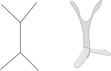
Figure 4.

Joyce made some additional arguments to suggest that this fattened discriminant locus must look fundamentally different in a neighbourhood of the two basic types of vertices we saw in §3, with the two types of vertices expected to appear pretty much as depicted in Figure 4. Thus the strong form of duality mentioned above, where we expect the discriminant loci of the special Lagrangian fibrations on a mirror pair to be the same, cannot hold. If this is the case, one needs to replace this strong form of duality with a weaker form.

It seems likely that the best way to rephrase the SYZ conjecture is in a limiting form. Mirror symmetry as we currently understand it has to do with degenerations of Calabi-Yau manifolds. Given a flat family $f:\mathcal{X}\rightarrow D$ over a disk $D$, with the fibre $\mathcal{X}_{0}$ over $0$ singular and all other fibres $n$-dimensional Calabi-Yau manifolds, we say the family is maximally unipotent if the monodromy transformation $T:H^{n}(\mathcal{X}_{t},\mathbb{Q})\rightarrow H^{n}(\mathcal{X}_{t},\mathbb{Q})$ ($t\in D$ non-zero) satisfies $(T-I)^{n+1}=0$ but $(T-I)^{n}\not=0$. It is a standard expectation of mirror symmetry that mirrors should be associated to maximally unipotent degenerations of Calabi-Yau manifolds. In particular, given two different maximally unipotent degenerations in a single complex moduli space for some Calabi-Yau manifold, one might obtain different mirror manifolds. Such degenerations are usually called “large complex structure limits” in the physics literature, although sometimes this phrase is used to impose some additional conditions on the degeneration, see [63].

We recall the definition of Gromov-Hausdorff convergence, a notion of convergence of a sequence of metric spaces.

Definition 5.2.

Let $(X,d_{X})$, $(Y,d_{Y})$ be two compact metric spaces. Suppose there exists maps $f:X\rightarrow Y$ and $g:Y\rightarrow X$ (not necessarily continuous) such that for all $x_{1},x_{2}\in X$,

$$|d_{X}(x_{1},x_{2})-d_{Y}(f(x_{1}),f(x_{2}))|<\epsilon$$

and for all $x\in X$,

$$d_{X}(x,g\circ f(x))<\epsilon,$$

and the two symmetric properties for $Y$ hold. Then we say the Gromov–Hausdorff distance between $X$ and $Y$ is at most $\epsilon$. The Gromov–Hausdorff distance $d_{GH}(X,Y)$ is the infimum of all such $\epsilon$.

It follows from results of Gromov (see for example [68], pg. 281, Cor. 1.11) that the space of compact Ricci-flat manifolds with diameter $\leq C$ is precompact with respect to Gromov-Hausdorff distance, i.e., any sequence of such manifolds has a subsequence converging with respect to the Gromov-Hausdorff distance to a metric space. This metric space could be quite bad; this is quite outside the realm of algebraic geometry! Nevertheless, this raises the following natural question. Given a maximally unipotent degeneration of Calabi-Yau manifolds $\mathcal{X}\rightarrow D$, take a sequence $t_{i}\in D$ converging to $0$, and consider a sequence $(\mathcal{X}_{t_{i}},g_{t_{i}})$, where $g_{t_{i}}$ is a choice of Ricci-flat metric chosen so that $Diam(g_{t_{i}})$ remains bounded. What is the Gromov-Hausdorff limit of $(\mathcal{X}_{t_{i}},g_{t_{i}})$, or the limit of some convergent subsequence?

Example 5.3.

Consider a degenerating family of elliptic curves parameterized by $t$, given by $\mathbb{C}/(\mathbb{Z}+\mathbb{Z}\tau)$ where $1$ and $\tau={1\over 2\pi i}\log t$ are periods of the elliptic curves. If we take $t$ approaching $0$ along the positive real axis, then we can just view this as a family of elliptic curves $\mathcal{X}_{\alpha}$ with period $1$ and $i\alpha$ with $\alpha\rightarrow\infty$. If we take the standard Euclidean metric $g$ on $\mathcal{X}_{\alpha}$, then the diameter of $\mathcal{X}_{\alpha}$ is unbounded. To obtain a bounded diameter, we replace $g$ by $g/\alpha^{2}$; equivalently, we can keep $g$ fixed on $\mathbb{C}$ but change the periods of the elliptic curve to $1/\alpha,i$. It then becomes clear that the Gromov-Hausdorff limit of such a sequence of elliptic curves is a circle $\mathbb{R}/\mathbb{Z}$.

This simple example motivates the first conjecture about maximally unipotent degenerations, conjectured independently by myself and Wilson on the one hand [38] and Kontsevich and Soibelman [53] on the other.

Conjecture 5.4.

Let $\mathcal{X}\rightarrow D$ be a maximally unipotent degeneration of simply-connected Calabi-Yau manifolds with full $SU(n)$ holonomy, $t_{i}\in D$ with $t_{i}\rightarrow 0$, and let $g_{i}$ be a Ricci-flat metric on $\mathcal{X}_{t_{i}}$ normalized to have fixed diameter $C$. Then a convergent subsequence of $(\mathcal{X}_{t_{i}},g_{i})$ converges to a metric space $(X_{\infty},d_{\infty})$, where $X_{\infty}$ is homeomorphic to $S^{n}$. Furthermore, $d_{\infty}$ is induced by a Riemannian metric on $X_{\infty}\setminus\Gamma$, where $\Gamma\subseteq X_{\infty}$ is a set of codimension two.

Here the topology of the limit depends on the nature of the non-singular fibres $\mathcal{X}_{t}$; for example, if instead $\mathcal{X}_{t}$ was hyperkähler, then we would expect the limit to be a projective space. Also, even in the case of full $SU(n)$ holonomy, if $\mathcal{X}_{t}$ is not simply connected, we would expect limits such as $\mathbb{Q}$-homology spheres to arise.

Conjecture 5.4 is directly inspired by the SYZ conjecture. Suppose we had special Lagrangian fibrations $f_{i}:\mathcal{X}_{t_{i}}\rightarrow B_{i}$. Then as the maximally unipotent degeneration is approached, one can see that the volume of the fibres of these fibrations goes to zero. This would suggest these fibres collapse, hopefully leaving the base as the limit.

This conjecture was proved by myself and Wilson in 2000 for K3 surfaces in [38]. The proof relied on a number of pleasant facts about K3 surfaces. First, they are hyperkähler manifolds, and a special Lagrangian torus fibration becomes an elliptic fibration after a hyperkähler rotation of the complex structure. Since it is easy to construct elliptic fibrations on K3 surfaces, and indeed such a fibration arises from the data of the maximally unipotent degeneration, it is easy to obtain a special Lagrangian fibration. Once this is done, one needs to carry out a detailed analysis of the behaviour of Ricci-flat metrics in the limit. This is done by creating good approximations to Ricci-flat metric, using the existence of explicit local models for these metrics near singular fibres of special Lagrangian fibrations in complex dimension two.

Most of the techniques used are not available in higher dimension. However, much more recently, weaker collapsing results in the hyperkähler case were obtained in work with V. Tosatti and Y. Zhang in [36], assuming the existence of abelian variety fibrations analogous to the elliptic fibrations in the K3 case. Rather than getting an explicit approximate Ricci-flat metric, we make use of a priori estimates of Tosatti in [76].

In the general Calabi-Yau case, the only progress towards the conjecture has been work of Zhang in [78] showing existence of special Lagrangian fibrations in regions of Calabi-Yau manifolds with bounded injectivity radius and sectional curvature and deduces local collapsing from the existence of special Lagrangian fibrations.

The motivation for Conjecture 5.4 from SYZ also provides a limiting form of the conjecture. There are any number of problems with trying to prove the existence of special Lagrangian fibrations on Calabi-Yau manifolds. Even the existence of a single special Lagrangian torus near a maximally unipotent degeneration is unknown, but we expect it should be easier to find them as we approach the maximally unipotent point. Furthermore, even if we find a special Lagrangian torus, we know that it moves in an $n$-dimensional family, but we don’t know its deformations fill out the entire manifold. In addition, there is no guarantee that even if it does, we obtain a foliation of the manifold: nearby special Lagrangian submanifolds may intersect. (For an example, see [60].) So instead, we will just look at the moduli space of special Lagrangian tori.

Given a maximally unipotent degeneration of Calabi-Yau manifolds of dimension $n$, it is known that the image of $(T-I)^{n}:H_{n}(\mathcal{X}_{t},\mathbb{Q})\rightarrow H_{n}(\mathcal{X}_{t},\mathbb{Q})$ is a one-dimensional subspace $W_{0}$. Suppose, given a sequence $t_{i}$ with $t_{i}\rightarrow 0$ as $i\rightarrow\infty$, that for $t_{i}$ sufficiently close to zero, there is a special Lagrangian $T^{n}$ which generates $W_{0}$. This is where we expect to find fibres of a special Lagrangian fibration associated to a maximally unipotent degeneration. Let $B_{0,i}$ be the moduli space of deformations of this torus; every point of $B_{0,i}$ corresponds to a smooth special Lagrangian torus in $\mathcal{X}_{t_{i}}$. This manifold then comes equipped with the McLean metric and affine structures defined in §2. One can then compactify $B_{0,i}\subseteq B_{i}$, (probably by taking the closure of $B_{0,i}$ in the space of special Lagrangian currents; the details aren’t important here). This gives a series of metric spaces $(B_{i},d_{i})$ with the metric $d_{i}$ induced by the McLean metric. If the McLean metric is normalized to keep the diameter of $B_{i}$ constant independent of $i$, then we can hope that $(B_{i},d_{i})$ converges to a compact metric space $(B_{\infty},d_{\infty})$. Here then is the limiting form of SYZ:

Conjecture 5.5.

If $(\mathcal{X}_{t_{i}},g_{i})$ converges to $(X_{\infty},g_{\infty})$ and $(B_{i},d_{i})$ is non-empty for large $i$ and converges to $(B_{\infty},d_{\infty})$, then $B_{\infty}$ and $X_{\infty}$ are isometric up to scaling. Furthermore, there is a subspace $B_{\infty,0}\subseteq B_{\infty}$ with $\Gamma:=B_{\infty}\setminus B_{\infty,0}$ of Hausdorff codimension 2 in $B_{\infty}$ such that $B_{\infty,0}$ is a Monge-Ampère manifold, with the Monge-Ampère metric inducing $d_{\infty}$ on $B_{\infty,0}$.

Essentially what this is saying is that as we approach the maximally unipotent degeneration, we expect to have a special Lagrangian fibration on larger and larger subsets of $\mathcal{X}_{t_{i}}$. Furthermore, in the limit, the codimension one discriminant locus suggested by Joyce converges to a codimension two discriminant locus, and (the not necessarily Monge-Ampère, see [60]) Hessian metrics on $B_{0,i}$ converge to a Monge-Ampère metric.

The main point I want to get at here is that it is likely the SYZ conjecture is only “approximately” correct, and one needs to look at the limit to have a hope of proving anything. On the other hand, the above conjecture seems likely to be accessible by currently understood techniques. I remain hopeful that this conjecture will be proved, though much additional work will be necessary.

How do we do mirror symmetry using this modified version of the SYZ conjecture? Essentially, we would follow these steps:

1. We begin with a maximally unipotent degeneration of Calabi-Yau manifolds $\mathcal{X}\rightarrow D$, along with a choice of polarization. This gives us a Kähler class $[\omega_{t}]\in H^{2}(\mathcal{X}_{t},\mathbb{R})$ for each $t\in D\setminus 0$, represented by $\omega_{t}$ the Kähler form of a Ricci-flat metric $g_{t}$.

2. Identify the Gromov-Hausdorff limit of a sequence $(\mathcal{X}_{t_{i}},r_{i}g_{t_{i}})$ where $t_{i}\rightarrow 0$ and $r_{i}$ is a scale factor which keeps the diameter of $\mathcal{X}_{t_{i}}$ constant. The limit will be, if the above conjectures work, an affine manifold with singularities $B$ along with a Monge-Ampère metric.

3. Perform a Legendre transform to obtain a new affine manifold with singularities $\check{B}$, though with the same metric.

4. Try to construct a compactification of $X_{\epsilon}(\check{B}_{0})$ for small $\epsilon>0$ to obtain a complex manifold $X_{\epsilon}(\check{B})$. This will be the mirror manifold.

As we shall see, we do not expect that we will need the full strength of steps (2) and (3) to carry out mirror symmetry; some way of identifying the base $B$ will be sufficient. Nevertheless, (2) is interesting from the point of view of understanding the differential geomtry of Ricci-flat Kähler manifolds.

Step (4), on the other hand, is crucial, and we need to elaborate on this last step a bit more. The problem is that while we expect that it should be possible in general to construct symplectic compactifications of the symplectic manifold $\check{X}(B_{0})$ (and hence get the mirror as a symplectic manifold, see [8] for the three-dimensional case), we don’t expect to be able to compactify $X_{\epsilon}(\check{B}_{0})$ as a complex manifold. Instead, the expectation is that a small deformation of $X_{\epsilon}(\check{B}_{0})$ is necessary before it can be compactified. Furthermore, this small deformation is critically important in mirror symmetry: it is this small deformation which provides the $B$-model instanton corrections.

Because this last item is so important, let’s give it a name:

Question 5.6 (The reconstruction problem, Version I).

Given a tropical affine manifold with singularities $B$, construct a complex manifold $X_{\epsilon}(B)$ which is a compactification of a small deformation of $X_{\epsilon}(B_{0})$.

We will return to this question later in the paper. However, I do not wish to dwell further on the differential-geometric versions of the SYZ conjecture here. Instead I will move on to describing how the above discussion motivated the algebro-geometric program developed by myself and Siebert for understanding mirror symmetry, and then describe recent work and ideas coming out of this program.

6. Gromov-Hausdorff limits, algebraic degenerations, and mirror symmetry

We now have two notions of limit: the familiar algebro-geometric notion of a degenerating family $\mathcal{X}\rightarrow D$ over a disk on the one hand, and the Gromov-Hausdorff limit on the other. In 2000 Kontsevich and Soibelman had an important insight (see [53]) into the connection between these two. In this section I will give a rough idea of how and why this works.

Very roughly speaking, the Gromov-Hausdorff limit $(\mathcal{X}_{t_{i}},g_{t_{i}})$ as $t_{i}\rightarrow 0$, or equivalently, the base of the putative SYZ fibration, should coincide, topologically, with the dual intersection complex of the singular fibre $\mathcal{X}_{0}$. More precisely, in a relatively simple situation, suppose $f:\mathcal{X}\rightarrow D$ is relatively minimal (in the sense of Mori) and normal crossings, with $\mathcal{X}_{0}$ having irreducible components $X_{1},\ldots,X_{m}$. The dual intersection complex of $\mathcal{X}_{0}$ is the simplicial complex with vertices $v_{1},\ldots,v_{m}$, and which contains a simplex $\langle v_{i_{0}},\ldots,v_{i_{p}}\rangle$ if $X_{i_{0}}\cap\cdots\cap X_{i_{p}}\not=\emptyset$. The idea that the dual intersection complex should play a role in describing the base of the SYZ fibration was perhaps first suggested by Leung and Vafa in [56].

Let us explain roughly why this should be, first by looking at a standard family of degenerating elliptic curves with periods $1$ and ${n\over 2\pi i}\log t$ for $n$ a positive integer. Such a family over the punctured disk is extended to a family over the disk by adding a Kodaira type $I_{n}$ (a cycle of $n$ rational curves) fibre over the origin.

Taking a sequence $t_{i}\rightarrow 0$ with $t_{i}$ real and positive gives a sequence of elliptic curves of the form $X_{\epsilon_{i}}(B)$ where $B=\mathbb{R}/n\mathbb{Z}$ and $\epsilon_{i}=-{2\pi\over\ln t_{i}}$. In addition, the metric on $X_{\epsilon_{i}}(B)$, properly scaled, comes from the constant Hessian metric on $B$. So we wish to explain how $B$ is related to the geometry near the singular fibre. To this end, let $X_{1},\ldots,X_{n}$ be the irreducible components of $\mathcal{X}_{0}$; these are all $\mathbb{P}^{1}$’s. Let $P_{1},\ldots,P_{n}$ be the singular points of $\mathcal{X}_{0}$.

We’ll consider two sorts of open sets in $\mathcal{X}$. For the first type, choose a coordinate $z$ on $X_{i}$, with $P_{i}$ given by $z=0$ and $P_{i+1}$ given by $z=\infty$. Let $U_{i}\subseteq X_{i}$ be the open set $\{z\,|\,\delta\leq|z|\leq 1/\delta\}$ for some small fixed $\delta$. Then one can find a neighbourhood $\widetilde{U}_{i}$ of $U_{i}$ in $\mathcal{X}$ such that $\widetilde{U}_{i}$ is biholomorphic to $U_{i}\times D_{\rho}$ for $\rho>0$ sufficiently small, $D_{\rho}$ a disk of radius $\rho$ in $\mathbb{C}$, and $f|_{\widetilde{U}_{i}}$ is the projection onto $D_{\rho}$.

On the other hand, each $P_{i}$ has a neighbourhood $\widetilde{V}_{i}$ in $\mathcal{X}$ biholomorphic to a polydisk $\{(z_{1},z_{2})\in\mathbb{C}^{2}\,|\,|z_{1}|\leq\delta^{\prime},|z_{2}|\leq\delta^{\prime}\}$ on which $f$ takes the form $z_{1}z_{2}$.

If $\delta$ and $\delta^{\prime}$ are chosen correctly, then for $t$ sufficiently close to zero,

$$\{\widetilde{V}_{i}\cap\mathcal{X}_{t}\,|\,1\leq i\leq n\}\cup\{\widetilde{U}_{i}\cap\mathcal{X}_{t}\,|\,1\leq i\leq n\}$$

form an open cover of $\mathcal{X}_{t}$. Now each of the sets in this open cover can be written as $X_{\epsilon}(U)$ for some $U$ a one-dimensional (non-compact) affine manifold and $\epsilon=-2\pi/\ln|t|$. If $U$ is an open interval $(a,b)\subseteq\mathbb{R}$, then $X_{\epsilon}(U)$ is biholomorphic to the annulus

$$\{z\in\mathbb{C}\,|\,e^{-2\pi b/\epsilon}\leq|z|\leq e^{-2\pi a/\epsilon}\}$$

as $q=e^{2\pi i(x+iy)/\epsilon}$ is a holomorphic coordinate on $X_{\epsilon}((a,b))$. Thus

$$\widetilde{U}_{i}\cap\mathcal{X}_{t}\cong X_{\epsilon}\left(\left({\epsilon\ln\delta\over 2\pi},-{\epsilon\ln\delta\over 2\pi}\right)\right)$$

with $\epsilon=-2\pi/\ln|t|$. As $t\rightarrow 0$, the interval $(\epsilon\ln\delta/2\pi,-\epsilon\ln\delta/2\pi)$ shrinks to a point. So $\widetilde{U}_{i}\cap\mathcal{X}_{t}$ is a smaller and smaller open subset of $\mathcal{X}_{t}$ as $t\rightarrow 0$ when we view things in this way. This argument suggests that every irreducible component should be associated to a point on $B$.

Now look at $\widetilde{V}_{i}\cap\mathcal{X}_{t}$. This is

$$\{(z_{1},z_{2})\in\mathbb{C}^{2}\,|\,|z_{1}|,|z_{2}|<\delta^{\prime},z_{1}z_{2}=t\} \cong \{z\in\mathbb{C}\,|\,|t|/\delta^{\prime}\leq|z|\leq\delta^{\prime}\}$$

$$\cong X_{\epsilon}\left({-\epsilon\over 2\pi}\ln\delta^{\prime},{\epsilon\over 2\pi}(\ln\delta^{\prime}-\ln|t|)\right)$$

with $\epsilon=-2\pi/\ln|t|$. This interval approaches the unit interval $(0,1)$ as $t\rightarrow 0$. So the open set $\widetilde{V}_{i}\cap\mathcal{X}_{t}$ ends up being a large portion of $\mathcal{X}_{t}$. We end up with $\mathcal{X}_{t}$, for small $t$, being a union of open sets of the form $X_{\epsilon}((i+\epsilon^{\prime},i+1-\epsilon^{\prime}))$ (i.e., $\widetilde{V}_{i}\cap\mathcal{X}_{\epsilon}$) and $X_{\epsilon}((i-\epsilon^{\prime\prime},i+\epsilon^{\prime\prime}))$ (i.e., $\widetilde{U}_{i}\cap\mathcal{X}_{t}$) for $\epsilon^{\prime}$, $\epsilon^{\prime\prime}$ sufficiently small. These should glue, at least approximately, to give $X_{\epsilon}(B)$. So we see that irreducible components of $\mathcal{X}_{0}$ seem to coincide with points on $B$, but intersections of components coincide with lines. In this way we see the dual intersection complex emerge.

Let us make one more observation before beginning with rigorous results in the next section. Suppose more generally we had a Gorenstein toroidal crossings degeneration of Calabi-Yau manifolds $f:\mathcal{X}\rightarrow D$ (see [73]). This means that every point $x\in\mathcal{X}$ has a neighbourhood isomorphic to an open set in an affine Gorenstein (i.e., the canonical class is a Cartier divisor) toric variety, with $f$ given locally by a monomial which vanishes exactly to order $1$ on each codimension one toric stratum. This is a generalization of the notion of normal crossings. Very roughly, the above argument suggests that each irreducible component of the central fibre will correspond to a point of the Gromov-Hausdorff limit. The following exercise shows what kind of contribution to $B$ to expect from a point $x\in\mathcal{X}_{0}$ which is a zero-dimensional stratum in $\mathcal{X}_{0}$.

Exercise 6.1.

Suppose that there is a point $x\in\mathcal{X}_{0}$ which has a neighbourhood isomorphic to a neighbourhood of a dimension zero torus orbit of an affine Gorenstein toric variety $Y_{x}$. Such an affine variety is specified as follows. Set $M=\mathbb{Z}^{n}$, $M_{\mathbb{R}}=M\otimes_{\mathbb{Z}}\mathbb{R}$, $N=\operatorname{Hom}_{\mathbb{Z}}(M,\mathbb{Z})$, $N_{\mathbb{R}}=N\otimes_{\mathbb{Z}}\mathbb{R}$ with $n=\dim\mathcal{X}_{t}$. Then there is a lattice polytope $\sigma\subseteq M_{\mathbb{R}}$, $C(\sigma):=\{(rm,r)\,|\,m\in\sigma,r\geq 0\}\subseteq M_{\mathbb{R}}\oplus\mathbb{R}$, $P:={C(\sigma)}^{\scriptscriptstyle\vee}\cap(N\oplus\mathbb{Z})$ the monoid determined by the dual of the cone $C(\sigma)$, $Y_{x}=\operatorname{Spec}\mathbb{C}[P]$, and finally $f$ coincides with the monomial $z^{(0,1)}$.

Now let us take a small neighbourhood of $x$ of the form

$$\widetilde{U}_{\delta}=\{y\in\operatorname{Spec}\mathbb{C}[P]\,|\,\hbox{$|z^{p}|<\delta$ for all $p\in P$}\}.$$

This is an open set as the condition $|z^{p}|<\delta$ can be tested on a finite generating set for $P$, provided that $\delta<1$. Then show that for a given $t$, $|t|<1$ and $\epsilon=-2\pi/\log|t|$, if

$$\sigma_{t}:=\{m\in M_{\mathbb{R}}\,|\,\hbox{$\langle p,(m,1)\rangle>{\log\delta\over\log|t|}$ for all $p\in P$}\},$$

then

$$f^{-1}(t)\cap\widetilde{U}_{\delta}\cong X_{\epsilon}(\sigma_{t}).$$

Note that

$$\sigma:=\{m\in M_{\mathbb{R}}\,|\,\hbox{$\langle p,(m,1)\rangle\geq 0$ for all $p\in P$}\},$$

so $\sigma_{t}$ is an open subset of $\sigma$, and as $t\rightarrow 0$, $\sigma_{t}$ converges to the interior of $\sigma$. ∎

This observation hopefully motivates the basic construction of the next section.

7. Toric degenerations, the intersection complex and its dual

I will now introduce the basic objects of the program developed by myself and Siebert to understand mirror symmetry in an algebro-geometric context. This program was announced in [29], and has been developed further in a series of papers [31], [32], [33], [22], [34], [28].

The motivation for this program came from two different directions. The first, which was largely my motivation, was the discussion of the limiting form of the SYZ conjecture of the previous sections. The second arose in work of Schröer and Siebert [72], [73], which led Siebert to the idea that log structures on degenerations of Calabi-Yau manifolds would allow one to view mirror symmetry as an operation performed on degenerate Calabi-Yau varieties. Siebert observed that at a combinatorial level, mirror symmetry exchanged data pertaining to the log structure and a polarization. This will be explained more clearly in the following section, when I introduce log structures. Together, Siebert and I realised that the combinatorial data he was considering could be encoded naturally in the dual intersection complex of the degeneration, which we saw in the previous section appears to be the base of the SYZ fibration. The combinatorial interchange of data necessary for mirror symmetry then corresponded to a discrete Legendre transform on the dual intersection complex. It became apparent that this approach provided an algebro-geometrization of the SYZ conjecture.

To set this up properly, one has to consider what kind of degenerations to allow. They should be maximally unipotent, of course, but there can be many different birational models of degenerations. Below we define the notion of toric degeneration. The class of toric degenerations may seem rather restrictive, but it appears to be the largest class of degenerations closed under mirror symmetry: one can construct the mirror of a toric degeneration as a toric degeneration. It does not appear that there is any other natural family of degenerations with this property. Much of the material in this section comes from [31], §4.

Roughly put, a toric degeneration of Calabi-Yau varieties is a degeneration whose central fibre is a union of toric varieties glued along toric strata, and the total space of the degeneration is, off of some well-behaved set $Z$ contained in the central fibre, locally toric with the family locally given by a monomial. The precise technical definition is as follows.

Definition 7.1.

Let $f:\mathcal{X}\rightarrow D$ be a proper flat family of relative dimension $n$, where $D$ is a disk and $\mathcal{X}$ is a complex analytic space (not necessarily non-singular). We say $f$ is a toric degeneration of Calabi-Yau varieties if

1. $\mathcal{X}_{t}$ is an irreducible normal Calabi-Yau variety with only canonical singularities for $t\not=0$. (The reader may like to assume $\mathcal{X}_{t}$ is smooth for $t\not=0$).

2. If $\nu:\widetilde{\mathcal{X}}_{0}\to\mathcal{X}_{0}$ is the normalization, then $\widetilde{\mathcal{X}}_{0}$ is a disjoint union of toric varieties, the conductor locus $C\subseteq\widetilde{\mathcal{X}}_{0}$ is reduced, and the map $C\to\nu(C)$ is unramified and generically two-to-one. (The conductor locus is a naturally defined scheme structure on the set where $\nu$ is not an isomorphism.) The square

   $$\begin{CD}C@>{}>{}>\widetilde{\mathcal{X}}_{0}\\ @V{}V{}V@V{}V{\nu}V\\ \nu(C)@>{}>{}>\mathcal{X}_{0}\end{CD}$$

   is cartesian and cocartesian.

3. $\mathcal{X}_{0}$ is a reduced Gorenstein space and the conductor locus $C$ restricted to each irreducible component of $\widetilde{\mathcal{X}}_{0}$ is the union of all toric Weil divisors of that component.

4. There exists a closed subset $Z\subseteq\mathcal{X}$ of relative codimension $\geq 2$ such that $Z$ satisfies the following properties: $Z$ does not contain the image under $\nu$ of any toric stratum of $\widetilde{\mathcal{X}}_{0}$, and for any point $x\in\mathcal{X}\setminus Z$, there is a neighbourhood $\widetilde{U}_{x}$ (in the analytic topology) of $x$, an $n+1$-dimensional affine toric variety $Y_{x}$, a regular function $f_{x}$ on $Y_{x}$ given by a monomial, and a commutative diagram

   $$\begin{matrix}\widetilde{U}_{x}&\smash{\mathop{\longrightarrow}\limits^{\psi_{x}}}&Y_{x}\cr\Big{\downarrow}\hbox to0.0pt{$\vbox{\hbox{$\scriptstyle f|_{\widetilde{U}_{x}}$}}$\hss}&&\Big{\downarrow}\hbox to0.0pt{$\vbox{\hbox{$\scriptstyle f_{x}$}}$\hss}\cr D^{\prime}&\smash{\mathop{\longrightarrow}\limits^{\varphi_{x}}}&\mathbb{C}\cr\end{matrix}$$

   where $\psi_{x}$ and $\varphi_{x}$ are open embeddings and $D^{\prime}\subseteq D$. Furthermore, $f_{x}$ vanishes precisely once on each toric divisor of $Y_{x}$.

Example 7.2.

Take $\mathcal{X}$ to be defined by the equation $tf_{4}+z_{0}z_{1}z_{2}z_{3}=0$ in $\mathbb{P}^{3}\times D$, where $D$ is a disk with coordinate $t$ and $f_{4}$ is a general homogeneous quartic polynomial on $\mathbb{P}^{3}$. It is easy to see that $\mathcal{X}$ is singular at the locus

$$\{t=f_{4}=0\}\cap Sing(\mathcal{X}_{0}).$$

As $\mathcal{X}_{0}$ is the coordinate tetrahedron, the singular locus of $\mathcal{X}_{0}$ consists of the six coordinate lines of $\mathbb{P}^{3}$, and $\mathcal{X}$ has four singular points along each such line, for a total of 24 singular points. Take $Z=Sing(\mathcal{X})$. Then away from $Z$, the projection $\mathcal{X}\rightarrow D$ is normal crossings, which yields condition (4) of the definition of toric degeneration. It is easy to see all other conditions are satisfied.

Given a toric degeneration $f:\mathcal{X}\rightarrow D$, we can build the dual intersection complex $(B,\mathscr{P})$ of $f$, as follows. Here $B$ is an integral affine manifold with singularities, and $\mathscr{P}$ is a polyhedral decomposition of $B$, i.e., a decomposition of $B$ into lattice polytopes. In fact, we will construct $B$ as a union of lattice polytopes. Specifically, let the normalisation of $\mathcal{X}_{0}$, $\widetilde{\mathcal{X}}_{0}$, be written as a disjoint union $\coprod X_{i}$ of toric varieties $X_{i}$, $\nu:\widetilde{\mathcal{X}}_{0}\rightarrow\mathcal{X}_{0}$ the normalisation. The strata of $\mathcal{X}_{0}$ are the elements of the set

$$Strata(\mathcal{X}_{0})=\{\nu(S)\,|\,\hbox{$S$ is a toric stratum of $X_{i}$ for some $i$}\}.$$

Here by toric stratum we mean the closure of a $(\mathbb{C}^{*})^{n}$ orbit.

Let $\{x\}\in Strata(\mathcal{X}_{0})$ be a zero-dimensional stratum. Applying Definition 7.1,(4), to a neighbourhood of $x$, there is a toric variety $Y_{x}$ such that in a neighbourhood of $x$, $f:\mathcal{X}\rightarrow D$ is locally isomorphic to $f_{x}:Y_{x}\rightarrow\mathbb{C}$, where $f_{x}$ is given by a monomial. Now the condition that $f_{x}$ vanishes precisely once along each toric divisor of $Y_{x}$ is the statement that $Y_{x}$ is Gorenstein, and as such, it arises as in Exercise 6.1. Indeed, let $M,N$ be given in Exercise 6.1, with $\operatorname{rank}M=\dim\mathcal{X}_{0}$. Then there is a lattice polytope $\sigma_{x}\subseteq M_{\mathbb{R}}$ such that $C(\sigma_{x})=\{(rm,r)|m\in\sigma,r\geq 0\}$ is the cone defining the toric variety $Y_{x}$. As we saw in Exercise 6.1, a small neighbourhood of $x$ in $\mathcal{X}$ should contribute a copy of $\sigma_{x}$ to $B$, which provides the motivation for our construction. We can now describe how to construct $B$ by gluing together the polytopes

$$\{\sigma_{x}\,|\,\{x\}\in Strata(\mathcal{X}_{0})\}.$$

We will do this in the case that every irreducible component of $\mathcal{X}_{0}$ is in fact itself normal so that $\nu:X_{i}\rightarrow\nu(X_{i})$ is an isomorphism. The reader may be able to imagine the more general construction. With this normality assumption, there is a one-to-one inclusion reversing correspondence between faces of $\sigma_{x}$ and elements of $Strata(\mathcal{X}_{0})$ containing $x$. We can then identify faces of $\sigma_{x}$ and $\sigma_{x^{\prime}}$ if they correspond to the same strata of $\mathcal{X}_{0}$. Some argument is necessary to show that this identification can be done via an integral affine transformation, but again this is not difficult.

Making these identifications, one obtains $B$. One can then prove

Lemma 7.3.

If $\mathcal{X}_{0}$ is complex $n$-dimensional, then $B$ is an real $n$-dimensional manifold.

See [31], Proposition 4.10 for a proof.

Now so far $B$ is just a topological manifold, constructed by gluing together lattice polytopes. Let

$$\mathscr{P}=\{\sigma\subseteq B|\hbox{$\sigma$ is a face of $\sigma_{x}$ for some zero-dimensional stratum $x$}\}.$$

There is a one-to-one inclusion reversing correspondence between strata of $\mathcal{X}_{0}$ and elements of $\mathscr{P}$.

It only remains to give $B$ an affine structure with singularities. In fact, I shall describe somewhat more structure on $B$ derived from $\mathcal{X}_{0}$ which in particular gives an affine structure with singularities on $B$.

First, for $\tau\in\mathscr{P}$, let

$$U_{\tau}:=\bigcup_{\{\sigma\in\mathscr{P}\,|\,\tau\subseteq\sigma\}}\operatorname{Int}(\sigma).$$

A fan structure along $\tau\in\mathscr{P}$ is a continuous map $S_{\tau}:U_{\tau}\rightarrow\mathbb{R}^{k}$ such that

1. $S_{\tau}^{-1}(0)=\operatorname{Int}(\tau)$.

2. If $e:\tau\rightarrow\sigma$ is an inclusion then $S_{\tau}|_{\operatorname{Int}\sigma}$ is an integral affine submersion onto its image.

3. The collection of cones

   $$\{K_{e}:=\mathbb{R}_{\geq 0}S_{\tau}(\sigma\cap U_{\tau})\,|\,e:\tau\rightarrow\sigma\}$$

   defines a finite fan $\Sigma_{\tau}$ in $\mathbb{R}^{k}$.

Two fan structures $S_{\tau},S^{\prime}_{\tau}:U_{\tau}\rightarrow\mathbb{R}^{k}$ are considered equivalent if they differ only by an integral linear transformation of $\mathbb{R}^{k}$.

If $S_{\tau}:U_{\tau}\rightarrow\mathbb{R}^{k}$ is a fan structure along $\tau\in\mathscr{P}$ and $\sigma\supseteq\tau$ then $U_{\sigma}\subseteq U_{\tau}$. The fan structure along $\sigma$ induced by $S_{\tau}$ is the composition

$$U_{\sigma}\smash{\mathop{\longrightarrow}\limits}U_{\tau}\smash{\mathop{\longrightarrow}\limits^{S_{\tau}}}\mathbb{R}^{k}\smash{\mathop{\longrightarrow}\limits}\mathbb{R}^{k}/L_{\sigma}\cong\mathbb{R}^{\ell}$$

where $L_{\sigma}\subseteq\mathbb{R}^{k}$ is the linear span of $S_{\tau}(\sigma)$.

Definition 7.4.

An integral tropical manifold of dimension $n$ is a pair $(B,\mathscr{P})$ as above along with a choice of fan structure $S_{v}$ at each vertex $v$ of $\mathscr{P}$, with the property that if $v,w\in\tau$, then the fan structures along $\tau$ induced by $S_{v}$ and $S_{w}$ are equivalent.

Such data gives $B$ the structure of an integral affine manifold with singularities. Let $\Gamma\subseteq B$ be the union of those cells of $\operatorname{Bar}(\mathscr{P})$ (the first barycentric subdivision of $\mathscr{P}$) which are not contained in maximal cells of $\mathscr{P}$ nor contain vertices of $\mathscr{P}$. Then $B_{0}:=B\setminus\Gamma$ can be covered by

$$\{\operatorname{Int}(\sigma)\,|\,\sigma\in\mathscr{P}_{\max}\}\cup\{W_{v}\,|\,\hbox{$v\in\mathscr{P}$ a vertex}\}$$

for certain open neighbourhoods $W_{v}$ of $v\in B$ contained in $U_{v}$. We define an affine structure on $B_{0}$ by giving $\operatorname{Int}(\sigma)$ the natural affine structure given by $\sigma$ being a lattice polytope, while $S_{v}:U_{v}\rightarrow\mathbb{R}^{n}$ restricts to an affine chart on $W_{v}$.

Finally, the point is that the structure of $\mathcal{X}_{0}$ gives rise to an integral tropical manifold structure on $(B,\mathscr{P})$. Indeed, each vertex $v\in\mathscr{P}$ corresponds to an irreducible component $X_{v}$ of $\mathcal{X}_{0}$ and this irreducible component is a toric variety with fan $\Sigma_{v}$ in $\mathbb{R}^{n}$. Furthermore, there is a one-to-one correspondence between $p$-dimensional cones of $\Sigma_{v}$ and $p$-dimensional cells of $\mathscr{P}$ containing $v$ as a vertex, as they both correspond to strata of $\mathcal{X}_{0}$ contained in $X_{v}$. There is then a continuous map

$$\psi_{v}:U_{v}\rightarrow\mathbb{R}^{n}$$

which takes $U_{v}\cap\sigma$, for any $\sigma\in\mathscr{P}$ containing $v$ as a vertex, into the corresponding cone of $\Sigma_{v}$ integral affine linearly. Such a map is uniquely determined by the combinatorial correspondence and the requirement that it be integral affine linear on each cell. These maps define a fan structure at each vertex. Furthermore, these fan structures are compatible in the sense that if $v,w\in\tau$, the two induced fan structures on $U_{\tau}$ are equivalent. This follows because there is a well-defined fan $\Sigma_{\tau}$ defining the stratum corresponding to $\tau$.

Example 7.5.

Let $f:\mathcal{X}\rightarrow D$ be a degeneration of elliptic curves to an $I_{n}$ fibre. Then $B$ is the circle $\mathbb{R}/n\mathbb{Z}$, decomposed by $\mathscr{P}$ into $n$ line segments of length one.

Example 7.6.

Continuing with Example 7.2, the dual intersection complex is the boundary of a tetrahedron, with each face affine isomorphic to a standard two-simplex, and the affine structure near each vertex makes the polyhedral decomposition look locally like the fan for $\mathbb{P}^{2}$. There is one singularity at the barycenter of each edge, and one can calculate that the monodromy of $\Lambda$ about each of these singularities is $\begin{pmatrix}1&4\\ 0&1\end{pmatrix}$ in a suitable basis.

Example 7.7.

Consider the polytope $\Delta$ of Example 3.2. The dual polytope $\nabla$ is the convex hull of the points $(-1,-1,-1,-1),(1,0,0,0),\ldots,(0,0,0,1)$. The corresponding projective toric variety $\mathbb{P}_{\nabla}$ has a crepant resolution $X_{\Sigma}\rightarrow\mathbb{P}_{\nabla}$ where $\Sigma$ is the fan consisting of cones over all elements of the decomposition $\mathscr{P}$ of $\partial\Delta$ as described in Example 3.2. Consider in $\mathbb{P}_{\nabla}\times\mathbb{A}^{1}$ the degenerating family $\mathcal{X}\rightarrow\mathbb{A}^{1}$ of Calabi-Yau manifolds given by

$$s_{0}+t\sum_{m\in\nabla\cap\mathbb{Z}^{4}}c_{m}s_{m}=0$$

where $s_{m}$ is the section of $\mathcal{O}_{\mathbb{P}_{\nabla}}(1)$ corresponding to $m\in\nabla\cap\mathbb{Z}^{4}$. Let $\widetilde{\mathcal{X}}$ be the proper transform of $\mathcal{X}$ in $X_{\Sigma}\times\mathbb{A}^{1}$. Then the family $\widetilde{\mathcal{X}}\rightarrow\mathbb{A}^{1}$ is a toric degeneration with general fibre the mirror quintic, and its dual intersection complex is the affine manifold $B$ constructed in Example 3.2.

Is the dual intersection complex the right affine manifold with singularities? The following theorem provides evidence for this, and gives the connection between this construction and the SYZ conjecture.

Theorem 7.8.

Let $\mathcal{X}\rightarrow D$ be a toric degeneration, with dual intersection complex $(B,\mathscr{P})$. Then there is an open set $U\subseteq B$ such that $B\setminus U$ retracts onto the discriminant locus $\Gamma$ of $B$, and an open subset $\mathscr{U}_{t}$ of $\mathcal{X}_{t}$ which is biholomorphic to a small deformation of a twist of $X_{\epsilon}(U)$, where $\epsilon=O(-1/\ln|t|)$.

We will not be precise here about what we mean by small deformation; by twist, we mean a twist of the complex structure of $X_{\epsilon}(U)$ by a $B$-field. See [29] for a much more precise statement; the above statement is meant to give a feel for what is true. The proof, along with much more precise statements, will eventually appear in [30].

If $\mathcal{X}\rightarrow D$ is a polarized toric degeneration, i.e., if there is a relatively ample line bundle $\mathcal{L}$ on $\mathcal{X}$, then we can construct another integral tropical manifold $(\check{B},\check{\mathscr{P}})$, which we call the intersection complex, as follows.

For each irreducible component $X_{i}$ of $\mathcal{X}_{0}$, $\mathcal{L}|_{X_{i}}$ is an ample line bundle on a toric variety. Let $\check{\sigma}_{i}\subseteq N_{\mathbb{R}}$ denote the Newton polytope of this line bundle. There is then a one-to-one inclusion preserving correspondence between strata of $\mathcal{X}_{0}$ contained in $X_{i}$ and faces of $\check{\sigma}_{i}$. We can then glue together the $\check{\sigma}_{i}$’s in the obvious way: if $Y$ is a codimension one stratum of $\mathcal{X}_{0}$, it is contained in two irreducible components $X_{i}$ and $X_{j}$, and defines faces of $\check{\sigma}_{i}$ and $\check{\sigma}_{j}$. These faces are affine isomorphic because they are both the Newton polytope of $\mathcal{L}|_{Y}$, and we can then identify them in the canonical way. Thus we obtain a topological space $\check{B}$ with a polyhedral decomposition $\check{\mathscr{P}}$.

To define the fan structure at a vertex $v\in\mathscr{P}$, note that such a vertex corresponds to a zero-dimensional stratum of $\mathcal{X}_{0}$, giving rise to a maximal cell $\sigma_{v}$ of the dual intersection complex. Take the fan structure at $v$ to be defined using the normal fan $\check{\Sigma}_{v}$ to $\sigma_{v}$. Then there is a one-to-one inclusion preserving correspondence between cones in $\check{\Sigma}_{v}$ and strata of $\mathcal{X}_{0}$ containing the stratum corresponding to $v$. This correspondence allows us to define a fan structure

$$S_{v}:U_{v}\rightarrow\mathbb{R}^{n}$$

which takes $U_{v}\cap\check{\sigma}$, for any $\check{\sigma}\in\check{\mathscr{P}}$ containing $v$ as a vertex, into the corresponding cone of $\check{\Sigma}_{v}$. One checks easily that this set of fan structures satisfies the definition of integral tropical manifold, and hence defines the intersection complex $(\check{B},\check{\mathscr{P}})$.

Analogously to Theorem 7.8, we expect

Conjecture 7.9.

Let $\mathcal{X}\rightarrow D$ be a polarized toric degeneration, with intersection complex $(\check{B},\check{\mathscr{P}})$. Let $\omega_{t}$ be a Kähler form on $\mathcal{X}_{t}$ representing the first Chern class of the polarization. Then there is an open set $\check{U}\subseteq\check{B}$ such that $\check{B}\setminus\check{U}$ retracts onto the discriminant locus $\Gamma$ of $\check{B}$, such that $\mathcal{X}_{t}$ is a symplectic compactification of $\check{X}(\check{U})$ for any $t$.

I don’t expect this to be particularly difficult: it should be amenable to the techniques of W.-D. Ruan [71], but such an approach has not been carried out in general.

The relationship between the intersection complex and the dual intersection complex can be made more precise by introducing multi-valued piecewise linear functions, in analogy with the multi-valued convex functions of Definition 1.3.

Definition 7.10.

Let $(B,\mathscr{P})$ be an integral tropical manifold. Then a multi-valued piecewise linear function $\varphi$ on $B$ is a collection of continuous functions on an open cover $\{(U_{i},\varphi_{i})\}$ such that $\varphi_{i}$ is affine linear on each cell of $\mathscr{P}$ intersecting $U_{i}$, and on $U_{i}\cap U_{j}$, $\varphi_{i}-\varphi_{j}$ is affine linear. Furthermore, for any $\tau\in\mathscr{P}$, let $S_{\tau}:U_{\tau}\rightarrow\mathbb{R}^{k}$ be the induced fan structure. Then there is a piecewise linear function $\varphi_{\tau}$ on the fan $\Sigma_{\tau}$ such that on $U_{i}\cap U_{\tau}$, $\varphi_{i}-\varphi_{\tau}\circ S_{\tau}$ is affine linear. Here we will always assume that each linear part of $\varphi_{i}$ has differential in $\check{\Lambda}$, i.e., $\varphi_{i}$ has integral slopes.

The rather technical condition on the local behaviour of each $\varphi_{i}$ on $U_{\tau}$ comes from the idea that such a multi-valued piecewise linear function is really just a collection of piecewise linear functions on the fans $\Sigma_{\tau}$ given by the fan structure of $(B,\mathscr{P})$. These functions need to satisfy some compatibility conditions, and this compatibility is motivated by the following discussion.

Suppose we are given a polarized toric degeneration $\mathcal{X}\rightarrow D$. We in fact obtain a multi-valued piecewise linear function $\varphi$ on the dual intersection complex $(B,\mathscr{P})$ as follows. Restricting to any toric stratum $X_{\tau}$, $\mathcal{L}|_{X_{\tau}}$ is determined completely by an integral piecewise linear function $\varphi_{\tau}$ on $\Sigma_{\tau}$, well-defined up to a choice of linear function. Pulling back this piecewise linear function via $S_{\tau}$ to $U_{\tau}$, we obtain a collection of piecewise linear functions $\{(U_{\tau},\varphi_{\tau}\circ S_{\tau})\,|\,\tau\in\mathscr{P}\}$. The fact that $(\mathcal{L}|_{X_{\tau}})|_{X_{\sigma}}=\mathcal{L}|_{X_{\sigma}}$ for $\tau\subseteq\sigma$ implies that on overlaps $\varphi_{\sigma}\circ S_{\sigma}$ and $\varphi_{\tau}\circ S_{\tau}$ differ by at most an affine linear function. So $\{(U_{\tau},\varphi_{\tau}\circ S_{\tau})\}$ defines a multi-valued piecewise linear function. The last condition in the definition of multi-valued piecewise linear function then reflects the need for the function to be locally a pull-back of a function via $S_{\sigma}$ in a neighbourhood of $\sigma$.

If $\mathcal{L}$ is ample, then the piecewise linear function determined by $\mathcal{L}|_{X_{\sigma}}$ is strictly convex. So we say a multi-valued piecewise linear function is strictly convex if $\varphi_{\tau}$ is strictly convex for each $\tau\in\mathscr{P}$.

As a consequence, if $\mathcal{X}\rightarrow D$ is a polarized toric degeneration, we will write $(B,\mathscr{P},\varphi)$ for the data of the dual intersection complex and the induced multi-valued function $\varphi$. We call this triple the dual intersection complex of the polarized degeneration.

Now suppose we are given abstractly a triple $(B,\mathscr{P},\varphi)$ with $(B,\mathscr{P})$ an integral tropical manifold and $\varphi$ a strictly convex multi-valued piecewise linear function on $B$. Then we construct the discrete Legendre transform $(\check{B},\check{\mathscr{P}},\check{\varphi})$ of $(B,\mathscr{P},\varphi)$ as follows.

$\check{B}$ will be constructed by gluing together Newton polytopes. If we view, for $v$ a vertex of $\mathscr{P}$, the fan $\Sigma_{v}$ as living in $M_{\mathbb{R}}$, then the Newton polytope of $\varphi_{v}$ is

$$\check{v}:=\{x\in N_{\mathbb{R}}\,|\,\langle x,y\rangle\geq-\varphi_{v}(y)\quad\forall y\in M_{\mathbb{R}}\}.$$

There is a one-to-one inclusion reversing correspondence between faces of $\check{v}$ and cells of $\mathscr{P}$ containing $v$. Furthermore, if $\sigma$ is the smallest cell of $\mathscr{P}$ containing two vertices $v$ and $v^{\prime}$, then the corresponding faces of $\check{v}$ and $\check{v}^{\prime}$ are integral affine isomorphic, as they are both isomorphic to the Newton polytope of $\varphi_{\sigma}$. Thus we can glue $\check{v}$ and $\check{v}^{\prime}$ along this common face. After making all these identifications, we obtain a cell complex $(\check{B},\check{\mathscr{P}})$, which is really just the dual cell complex of $(B,\mathscr{P})$. This is given an integral tropical structure by taking the fan structure at a vertex $\check{\sigma}$, for $\sigma\in\mathscr{P}_{\max}$, to be given by the normal fan to $\sigma$.

Finally, the function $\varphi$ has a discrete Legendre transform $\check{\varphi}$ on $(\check{B},\check{\mathscr{P}})$. We have no choice but to define $\check{\varphi}$ in a neighbourhood of a vertex $\check{\sigma}\in\check{\mathscr{P}}$ dual to a maximal cell $\sigma\in\mathscr{P}$ to be a piecewise linear function whose Newton polytope is $\sigma$, i.e.,

$$\check{\varphi}_{\check{\sigma}}(y)=-\inf\{\langle y,x\rangle\,|\,x\in\sigma\subseteq M_{\mathbb{R}}\}.$$

This gives $(\check{B},\check{\mathscr{P}},\check{\varphi})$, the discrete Legendre transform of $(B,\mathscr{P},\varphi)$. If $B$ is $\mathbb{R}^{n}$, then this coincides with the classical notion of discrete Legendre transform. The discrete Legendre transform has several relevant properties:

• The discrete Legendre transform of $(\check{B},\check{\mathscr{P}},\check{\varphi})$ is $(B,\mathscr{P},\varphi)$.

• If we view the underlying topological spaces $B$ and $\check{B}$ as identified by being the underlying space of dual cell complexes, then $\Lambda_{B_{0}}\cong\check{\Lambda}_{\check{B}_{0}}$ and $\check{\Lambda}_{B_{0}}\cong\Lambda_{\check{B}_{0}}$, where the subscript denotes which affine structure is being used to define $\Lambda$ or $\check{\Lambda}$.

This hopefully makes it clear that the discrete Legendre transform is a suitable replacement for the duality provided by the Legendre transform of §2.

Note in particular that if $\mathcal{X}\rightarrow D$ is a polarized toric degeneration, with dual intersection complex $(B,\mathscr{P},\varphi)$, then the discrete Legendre transform $(\check{B},\check{\mathscr{P}},\check{\varphi})$ satisfies the condition that $(\check{B},\check{\mathscr{P}})$ is the intersection complex of the polarized degeneration. The function $\check{\varphi}$ is some extra information on $\check{B}$, which from the definition of discrete Legendre transform encodes the cells of $\mathscr{P}$. These cells of the dual intersection complex were defined using the local toric structure of $\mathcal{X}\rightarrow D$. So $\check{\varphi}$ can be seen as carrying information about this local toric structure. We will say $(\check{B},\check{\mathscr{P}},\check{\varphi})$ is the intersection complex of the polarized toric degeneration $\mathcal{X}\rightarrow D$.

So we see that for $(B,\mathscr{P},\varphi)$, $\mathscr{P}$ carries information about the log structure and $\varphi$ carries information about the polarization, but for $(\check{B},\check{\mathscr{P}},\check{\varphi})$, $\check{\mathscr{P}}$ carries information about the polarization and $\check{\varphi}$ carries information about the log structure. Mirror symmetry interchanges these two pieces of information!

We can now state an algebro-geometric SYZ procedure. In analogy with the procedure suggested in §5, we could follow these steps:

1. We begin with a toric degeneration of Calabi-Yau manifolds $\mathcal{X}\rightarrow D$ with an ample polarization.

2. Construct the dual intersection complex $(B,\mathscr{P},\varphi)$ from this data, as explained above.

3. Perform the discrete Legendre transform to obtain $(\check{B},\check{\mathscr{P}},\check{\varphi})$.

4. Try to construct a polarized degeneration of Calabi-Yau manifolds $\check{\mathcal{X}}\rightarrow D$ whose dual intersection complex is $(\check{B},\check{\mathscr{P}},\check{\varphi})$, or whose intersection complex is $(B,\mathscr{P},\varphi)$.

Example 7.11.

The discrete Legendre transform enables us to reproduce Batyrev duality [5]. Let $\Delta\subseteq M_{\mathbb{R}}$ be a reflexive polytope, $\nabla\subseteq N_{\mathbb{R}}$ the polar dual, and assume $0\in\Delta$ is the unique interior point. We then obtain two toric degenerations given by the equations

$$s_{0}+t\sum_{m\in M\cap\Delta}c_{m}s_{m}=0,\quad\quad s_{0}+t\sum_{n\in N\cap\nabla}c_{n}s_{n}=0$$

in $\mathbb{P}_{\Delta}\times\mathbb{A}^{1}$ and $\mathbb{P}_{\nabla}\times\mathbb{A}^{1}$ respectively, with $s_{m}$ ($s_{n}$) the section of $\mathcal{O}_{\mathbb{P}_{\Delta}}(1)$ corresponding to $m$ (the section of $\mathcal{O}_{\mathbb{P}_{\nabla}}(1)$ corresponding to $n$). It is easy to check that the dual intersection complexes of these two degenerations are given as follows. For the first degeneration, $B=\partial\nabla$ with polyhedral decomposition given by the proper faces of $\nabla$. The fan structure at each vertex $v$ is given by projection $U_{v}\hookrightarrow N_{\mathbb{R}}\rightarrow N_{\mathbb{R}}/\mathbb{R}v$. For the second degeneration, one uses $\Delta$ instead of $\nabla$. One can then check that if one polarizes the two degenerations using $\mathcal{O}_{\mathbb{P}_{\Delta}}(1)$ and $\mathcal{O}_{\mathbb{P}_{\nabla}}(1)$ respectively, then the corresponding triples $(B,\mathscr{P},\varphi)$ are Legendre dual. Thus Batyrev duality is a special case of this general approach to a mirror construction.

For a much more general construction which works for the Batyrev-Borisov construction [6] of mirrors of complete intersection Calabi-Yaus in toric varieties, see [22].

The only step missing in this mirror symmetry algorithm is the last:

Question 7.12 (The reconstruction problem, Version II).

Given $(B,\mathscr{P},\varphi)$, is it possible to construct a polarized toric degeneration $\mathcal{X}\rightarrow D$ whose intersection complex is $(B,\mathscr{P},\varphi)$?

One could hope to solve this problem via naive deformation theory, by constructing the central fibre $\mathcal{X}_{0}$ from the data $(B,\mathscr{P},\varphi)$, and then deforming this to find a smoothing. However, as initially observed in the normal crossings case by Kawamata and Namikawa in [51], one needs to put some additional structure on $\mathcal{X}_{0}$ before it has good deformation theory. This structure is a log structure, and introducing log structures allows us to study many aspects of mirror symmetry directly on the degenerate fibre itself. So let us turn to a review of the theory of logarithmic structures.

8. Log structures

We review the notion of log structures of Fontaine-Illusie and Kato ([45], [50]). These play a key role in trying to understand mirror symmetry via degenerations.

Definition 8.1.

A log structure on a scheme (or analytic space) $X$ is a (unital) homomorphism

$$\alpha_{X}:\mathcal{M}_{X}\rightarrow\mathcal{O}_{X}$$

of sheaves of (multiplicative and commutative) monoids inducing an isomorphism $\alpha_{X}^{-1}(\mathcal{O}_{X}^{\times})\rightarrow\mathcal{O}_{X}^{\times}$. The monoid structure on $\mathcal{O}_{X}$ is given by multiplication. The triple $(X,\mathcal{M}_{X},\alpha_{X})$ is then called a log space. We often write the whole package as $X^{\dagger}$.

A morphism of log spaces $F:X^{\dagger}\rightarrow Y^{\dagger}$ consists of a morphism $\underline{F}:X\rightarrow Y$ of underlying spaces together with a homomorphism $F^{\#}:\underline{F}^{-1}(\mathcal{M}_{Y})\rightarrow\mathcal{M}_{X}$ commuting with the structure homomorphisms:

$$\alpha_{X}\circ F^{\#}=\underline{F}^{*}\circ\alpha_{Y}.$$

The key examples:

Examples 8.2.

(1) Let $X$ be a scheme and $Y\subseteq X$ a closed subset of codimension one. Denote by $j:X\setminus Y\rightarrow X$ the inclusion. Then the inclusion

$$\alpha_{X}:\mathcal{M}_{X}=j_{*}(\mathcal{O}_{X\setminus Y}^{\times})\cap\mathcal{O}_{X}\rightarrow\mathcal{O}_{X}$$

of the sheaf of regular functions invertible off of $Y$ is a log structure on $X$. This is called a divisorial log structure on $X$.

(2) A prelog structure, i.e., an arbitrary homomorphism of sheaves of monoids $\varphi:\mathcal{P}\rightarrow\mathcal{O}_{X}$, defines an associated log structure $\mathcal{M}_{X}$ by

$$\mathcal{M}_{X}=(\mathcal{P}\oplus\mathcal{O}_{X}^{\times})/\{(p,\varphi(p)^{-1})\,|\,p\in\varphi^{-1}(\mathcal{O}_{X}^{\times})\}$$

and $\alpha_{X}(p,h)=h\cdot\varphi(p)$.

(3) If $f:X\rightarrow Y$ is a morphism of schemes and $\alpha_{Y}:\mathcal{M}_{Y}\rightarrow\mathcal{O}_{Y}$ is a log structure on $Y$, then the prelog structure $f^{-1}(\mathcal{M}_{Y})\rightarrow\mathcal{O}_{X}$ given as the composition of $\alpha_{Y}:f^{-1}(\mathcal{M}_{Y})\rightarrow f^{-1}\mathcal{O}_{Y}$ and $f^{*}:f^{-1}\mathcal{O}_{Y}\rightarrow\mathcal{O}_{X}$ defines an associated log structure on $X$, the pull-back log structure.

(4) In (1) we can pull back the log structure on $X$ to $Y$ using (3). Thus in particular, if $\mathcal{X}\rightarrow D$ is a toric degeneration, the inclusion $\mathcal{X}_{0}\subseteq\mathcal{X}$ gives a log structure on $\mathcal{X}$ and an induced log structure on $\mathcal{X}_{0}$. Similarly the inclusion $0\in D$ gives a log structure on $D$ and an induced one on $0$. Here $\mathcal{M}_{0}=\mathbb{C}^{\times}\oplus\mathbb{N}$, where $\mathbb{N}$ is the (additive) monoid of natural (non-negative) numbers, and

$$\alpha_{0}(h,n)=\begin{cases}h&n=0\\ 0&n\not=0.\end{cases}$$

$0^{\dagger}$ is usually called the standard log point.

We then have log morphisms $\mathcal{X}^{\dagger}\rightarrow D^{\dagger}$ and $\mathcal{X}_{0}^{\dagger}\rightarrow 0^{\dagger}$.

(5) If $\sigma\subseteq M_{\mathbb{R}}=\mathbb{R}^{n}$ is a strictly convex rational polyhedral cone, ${\sigma}^{\scriptscriptstyle\vee}\subseteq N_{\mathbb{R}}$ the dual cone, let $P={\sigma}^{\scriptscriptstyle\vee}\cap N$: this is a monoid under addition. The affine toric variety defined by $\sigma$ can be written as $X=\operatorname{Spec}\mathbb{C}[P]$. We then have a pre-log structure induced by the homomorphism of monoids

$$P\rightarrow\mathbb{C}[P]$$

given by $p\mapsto z^{p}$. There is then an associated log structure on $X$. This is in fact the same as the log structure induced by $\partial X\subseteq X$, where $\partial X$ is the toric boundary of $X$, i.e., the union of toric divisors of $X$.

If $p\in P$, then the monomial $z^{p}$ defines a map $f:X\rightarrow\operatorname{Spec}\mathbb{C}[\mathbb{N}]=\mathbb{A}^{1}$ which is a log morphism with the log structure on $\operatorname{Spec}\mathbb{C}[\mathbb{N}]$ induced similarly by $\mathbb{N}\rightarrow\mathbb{C}[\mathbb{N}]$. The fibre $X_{0}=\operatorname{Spec}\mathbb{C}[P]/(z^{p})$ is a subscheme of $X$, there is an induced log structure on $X_{0}$, and a map $X_{0}^{\dagger}\rightarrow 0^{\dagger}$ as in (4). The log morphism $f$ is an example of a log smooth morphism, see Definition 8.3.

Condition (4) of Definition 7.1 in fact implies that locally, away from $Z$, $\mathcal{X}^{\dagger}$ and $\mathcal{X}_{0}^{\dagger}$ are of the above form. So we should view $\mathcal{X}^{\dagger}\rightarrow D^{\dagger}$ as log smooth away from $Z$, and from the log point of view, $\mathcal{X}_{0}^{\dagger}$ can be treated much like a non-singular scheme away from $Z$.

(6) Given a monoid $P$ as in (5) and a morphism $X\rightarrow\operatorname{Spec}\mathbb{C}[P]$, we can pull back the log structure defined above on $\operatorname{Spec}\mathbb{C}[P]$ to $X$. If $X^{\dagger}$ is a log scheme which étale locally can be described in this way, we say $X^{\dagger}$ is a fine saturated log scheme. The adjective “fine” tells us it is locally described via maps to schemes of the form $\operatorname{Spec}\mathbb{C}[P]$ where $P$ is a finitely generated integral monoid, i.e., the canonical homomorphism $P\rightarrow P^{{\operatorname{gp}}}$ is an injection. The adjective “saturated” tells us the monoid $P$ is saturated. This means that $P$ is integral and whenever $p\in P^{{\operatorname{gp}}}$ satisfies $mp\in P$ for some $m>0$, $p\in P$. Such monoids arise, e.g., as the intersection of a rational polyhedral cone with a lattice.

Most of the literature on log geometry tends to apply only to fine log structures. In the key example of $\mathcal{X}_{0}^{\dagger}\rightarrow 0^{\dagger}$, the log structure is fine saturated away from the set $Z$. However, it is not in general fine along $Z$, and this tends to cause many technical problems as new techniques have to be developed to deal properly with the log structure along $Z$. ∎

The notion of log smoothness generalizes the morphisms of Examples 8.2, (5):

Definition 8.3.

A morphism $f:X^{\dagger}\rightarrow Y^{\dagger}$ of fine log schemes is log smooth if étale locally on $X$ and $Y$ it fits into a commutative diagram

with the following properties:

1. The canonical log structure on $\operatorname{Spec}\mathbb{Z}[P]$ and $\operatorname{Spec}\mathbb{Z}[Q]$ of Examples 8.2, (5), pull-back to the log structures on $X$ and $Y$ respectively.

2. The induced morphism

   $$X\rightarrow Y\times_{\operatorname{Spec}\mathbb{Z}[Q]}\operatorname{Spec}\mathbb{Z}[P]$$

   is a smooth morphism of schemes.

3. The right-hand vertical arrow is induced by a monoid homomorphism $Q\rightarrow P$ with $\operatorname{ker}(Q^{{\operatorname{gp}}}\rightarrow P^{{\operatorname{gp}}})$ and the torsion part of $\operatorname{coker}(Q^{{\operatorname{gp}}}\rightarrow P^{{\operatorname{gp}}})$ finite groups of orders invertible on $X$. Here $P^{{\operatorname{gp}}}$ denotes the Grothendieck group of $P$.

Log smooth morphisms include, in the simplest case, normal crossings morphisms.

On a log scheme $X^{\dagger}$ there is always an exact sequence

$$1\smash{\mathop{\longrightarrow}\limits}\mathcal{O}_{X}^{\times}\smash{\mathop{\longrightarrow}\limits^{\alpha^{-1}}}\mathcal{M}_{X}\smash{\mathop{\longrightarrow}\limits}\overline{\mathcal{M}}_{X}\smash{\mathop{\longrightarrow}\limits}0,$$

where we write the quotient sheaf of monoids $\overline{\mathcal{M}}_{X}$ additively. We call $\overline{\mathcal{M}}_{X}$ the ghost sheaf of the log structure. I like to view $\overline{\mathcal{M}}_{X}$ as specifying the combinatorial information associated to the log structure. For example, if $X^{\dagger}$ is induced by the Cartier divisor $Y\subseteq X$ with $X$ normal, then the stalk $\overline{\mathcal{M}}_{X,x}$ at $x\in X$ is the monoid of effective Cartier divisors on a neighbourhood of $x$ supported on $Y$.

It is useful for understanding pull-backs of log structures to note that if $f:Y\rightarrow X$ is a morphism with $X$ carrying a log structure, and $Y$ is given the pull-back log structure, then $\overline{\mathcal{M}}_{Y}=f^{-1}\overline{\mathcal{M}}_{X}$. In the case that $\mathcal{M}_{X}$ is induced by an inclusion of $Y\subseteq X$, $\overline{\mathcal{M}}_{X}$ is supported on $Y$, so we can equate $\overline{\mathcal{M}}_{X}$ and $\overline{\mathcal{M}}_{Y}$, the ghost sheaves for the divisorial log structure on $X$ and its restriction to $Y$.

Exercise 8.4.

Show that in Example 8.2, (5), $\overline{\mathcal{M}}_{X,x}=P$ if $\dim\sigma=\dim M_{\mathbb{R}}$ and $x$ is the unique zero-dimensional torus orbit of $X$. More generally,

$$\overline{\mathcal{M}}_{X,x}={{\tau}^{\scriptscriptstyle\vee}\cap N\over\tau^{\perp}\cap N}=\operatorname{Hom}_{monoid}(\tau\cap M,\mathbb{N}),$$

when $x\in X$ is in the torus orbit corresponding to a face $\tau$ of $\sigma$. In particular, $\tau$ can be recovered as $\operatorname{Hom}_{monoid}(\overline{\mathcal{M}}_{X,x},\mathbb{R}_{\geq 0})$, where $\mathbb{R}_{\geq 0}$ is the additive monoid of non-negative real numbers. ∎

In the sections which follow, the key logarithmic spaces we consider will be those arising from toric degenerations $\mathcal{X}\rightarrow D$. As above, the central fibre $\mathcal{X}_{0}\subseteq\mathcal{X}$ induces a divisorial log structure on $\mathcal{X}$, and restricting gives a log scheme $\mathcal{X}_{0}^{\dagger}$ along with a morphism $\mathcal{X}_{0}^{\dagger}\rightarrow 0^{\dagger}$ which is log smooth off of the bad set $Z\subseteq\mathcal{X}_{0}$.

We can now elaborate on the philosophy we wish to take with the following diagram:

There are two sides to mirror symmetry. The $A$-model side involves counting curves: we wish to count curves in the general fibre of a toric degeneration $\mathcal{X}\rightarrow D$. There are good reasons to believe that this count can in fact be performed on $\mathcal{X}_{0}^{\dagger}$, using a theory of logarithmic Gromov-Witten invariants: see §9. The hope is that $\mathcal{X}_{0}$ is a sufficiently combinatorial object so that such a count can be carried out in a combinatorial manner.

The $B$-side involves deformations of complex structure. The idea is that to understand deformations of complex structure, we should start with the central fibre $\mathcal{X}_{0}^{\dagger}$ and try to construct smoothings, i.e., construct a toric degeneration with this central fibre. The log structure is necessary to find a unique smoothing. If this smoothing can be described sufficiently explicitly, then again one should be able to extract the necessary periods for the $B$-model calculations purely in terms of combinatorics.

So log geometry will play an important role on both sides of mirror symmetry, but as the above suggests, there should be some combinatorial objects underlying both calculations.

In fact, log geometry is closely related to tropical geometry. We will explore in the following sections how tropical geometry controls both the $A$- and $B$-model sides of the above picture, completing the above diagram:

9. The $A$-model and tropical geometry

The first link between log geometry and tropical geometry comes from an elementary combinatorial construction. Given a log scheme $X^{\dagger}$, we can construct the tropicalization of $X^{\dagger}$, as follows. For each geometric point $\bar{\eta}$ of $X$, we have a monoid $\overline{\mathcal{M}}_{X,\bar{\eta}}$, and hence a cone $C_{\bar{\eta}}:=\operatorname{Hom}(\overline{\mathcal{M}}_{X,\bar{\eta}},\mathbb{R}_{\geq 0})$ (where here $\operatorname{Hom}$ denotes monoid homomorphisms and $\mathbb{R}_{\geq 0}$ is given the additive monoid structure). Further, if $\bar{\eta}$ is in the closure of $\bar{\eta}^{\prime}$, there is a generization map $\overline{\mathcal{M}}_{X,\bar{\eta}}\rightarrow\overline{\mathcal{M}}_{X,\bar{\eta}^{\prime}}$. Dualizing, this gives maps $C_{\bar{\eta}^{\prime}}\rightarrow C_{\bar{\eta}}$. If the log structure on $X$ is fine, then these maps are inclusions of faces of strictly convex rational polyhedral cones. We can then form a cell complex by making identifications given by these inclusions of faces, obtaining a polyhedral cone complex $\mathrm{Trop}(X^{\dagger})$. Actually, in general this may not really make sense as a cell complex because the generization maps may induce many strange self-identifications on faces, but in the situations we want to describe here, this will not cause a problem.

This construction is functorial, so if $f:X^{\dagger}\rightarrow Y^{\dagger}$ is a morphism of log schemes, then we obtain $\mathrm{Trop}(f):\mathrm{Trop}(X^{\dagger})\rightarrow\mathrm{Trop}(Y^{\dagger})$.

For example, consider the case of a toric degeneration $\mathcal{X}\rightarrow D$. As we saw in the previous section, this gives a morphism of log schemes $\mathcal{X}_{0}^{\dagger}\rightarrow 0^{\dagger}$. The bad set $Z\subseteq\mathcal{X}_{0}$ is precisely the locus where the log structure on $\mathcal{X}_{0}$ is not fine. Thus we can apply the above tropicalization construction to $\mathcal{X}_{0}^{\dagger}\setminus Z\rightarrow 0^{\dagger}$. Now $\mathrm{Trop}(0^{\dagger})=\mathbb{R}_{\geq 0}$ is a ray. On the other hand, if $x\in\mathcal{X}_{0}$ is a zero-dimensional stratum, locally a neighbourhood of $x$ looks like the fibre over $0$ of $f_{x}:Y_{x}\rightarrow\mathbb{C}$ where $Y_{x}$ is a toric variety defined by $C(\sigma_{x})\subseteq M_{\mathbb{R}}\oplus\mathbb{R}$ for a lattice polytope $\sigma_{x}\subseteq M_{\mathbb{R}}$, and the morphism $Y_{x}\rightarrow\mathbb{C}$ is given by the projection $M_{\mathbb{R}}\oplus\mathbb{R}\rightarrow\mathbb{R}$. Then $\overline{\mathcal{M}}_{\mathcal{X}_{0},x}=C(\sigma_{x})^{\vee}\cap(N\oplus\mathbb{Z})$, as follows from Exercise 8.4, and $C_{x}=C(\sigma_{x})$. In particular, the induced map $\mathrm{Trop}(f):C_{x}\rightarrow\mathrm{Trop}(0^{\dagger})$ has fibre $\mathrm{Trop}(f)^{-1}(1)=\sigma_{x}$. From this, one checks easily that

$$\mathrm{Trop}(f):\mathrm{Trop}(\mathcal{X}_{0}^{\dagger}\setminus Z)\rightarrow\mathrm{Trop}(0^{\dagger})=\mathbb{R}_{\geq 0}$$

has fibre

$$\mathrm{Trop}(f)^{-1}(1)=B,$$

with $B$ coming with the polyhedral decomposition $\mathscr{P}$. So the dual intersection complex comes from a very general construction. In particular, note that $B$ only depends on $\mathcal{X}_{0}^{\dagger}$, not on $\mathcal{X}$ (although this is obvious without knowing this general construction).

Now let us turn to the $A$-model, which for the purposes of this discussion means counting curves on Calabi-Yau manifolds. Suppose we have a toric degeneration $\mathcal{X}\rightarrow D$. We would like to count curves on the general fibre. Can we do so by counting curves on $\mathcal{X}_{0}$ instead, where the problem might have a more combinatorial nature?

This question has a long history. The first work on this kind of question was due to Li and Ruan [58] and Ionel and Parker [46],[47]. Essentially they considered a situation where one has a degeneration $\mathcal{X}\rightarrow D$ where the special fibre $\mathcal{X}_{0}=X_{1}\cup X_{2}$ is a normal crossings union of two smooth irreducible components. They showed that there was a theory of Gromov-Witten invariants of $\mathcal{X}_{0}$, and that it gave the same answer as Gromov-Witten theory on a general fibre. Further, they gave gluing formulas, which stated that the Gromov-Witten invariants of $\mathcal{X}_{0}$ could be computed using the Gromov-Witten invariants of the two pairs $(X_{i},X_{1}\cap X_{2})$, $i=1,2$. Here the Gromov-Witten theory associated to a pair $(X,D)$ where $D\subseteq X$ is a smooth divisor is the theory of relative Gromov-Witten invariants, where one considers curves in $X$ with some imposed orders of tangency at points on the curve with $D$. This gluing formula has proven to be a very powerful tool in Gromov-Witten theory.

In 2001, Bernd Siebert [74] proposed using log geometry to generalize these results. Meanwhile, Jun Li was working on an algebro-geometric approach to the Li-Ruan and Ionel-Parker theories (which were carried out using symplectic techniques). He gave a satisfactory algebro-geometric definition of relative Gromov-Witten invariants and reproved the gluing formula, using a few techniques from log geometry. However, the theory possesses a technical difficulty. In Gromov-Witten theory, it is standard that one allows the domain curves to develop bubbles. But in relative Gromov-Witten theory, it is also necessary to allow the target space $X$ to develop bubbles. This occurs when an irreducible component of the domain curve falls into the divisor $D$, so that the order of tangency with $D$ becomes meaningless. So the actual target space for a relative stable map might be $X$ with a chain of $\mathbb{P}^{1}$-bundles over $D$ glued to $D\subseteq X$. This often makes the analysis more difficult, and was a major stumbling block for extending these techniques to more complicated degenerations.

Several solutions to this problem were completed in 2011. Brett Parker in [66], [67] provided a completely new category, the category of exploded manifolds, in which to study Gromov-Witten theory. These manifolds carry information similar to log spaces, but is a somewhat more flexible and “softer” category in which to work. In [67] he provides a definition of Gromov-witten invariants in this setting and gives a gluing formula. Also, Siebert and I [34] completed a theory of logarithmic Gromov-Witten invariants, as did Abramovich and Chen [11],[1], working with Siebert’s original suggestion. I will summarize the basic ideas here.

Definition 9.1.

A log curve over a fine saturated log scheme $W^{\dagger}$ is a fine saturated log scheme $C^{\dagger}$ with a morphism $C^{\dagger}\rightarrow W^{\dagger}$ which is flat of relative dimension one, log smooth, and with all geometric fibres reduced.

Here log smoothness implies that the geometric fibres of $C\rightarrow W$ are nodal curves, which is pleasant as this is precisely the sort of curve which is allowed as the domain of a stable map. The log structure can also be viewed as incorporating marked points. For example, given a smooth curve $C$ over $W=\operatorname{Spec}\mathbb{C}$, one can take a finite number of points $x_{1},\ldots,x_{k}\in C$ and give $C$ the divisorial log structure associated to the subset $\{x_{1},\ldots,x_{k}\}\subseteq C$. Then $C^{\dagger}$ is log smooth over $W$ with the trivial log structure $\mathcal{M}_{W}=\mathcal{O}_{W}^{\times}$.

Definition 9.2.

Let $X^{\dagger}\rightarrow S^{\dagger}$ be a morphism of fine saturated log schemes. A log curve in $X^{\dagger}$ with base $W^{\dagger}$ is a log curve $C^{\dagger}/W^{\dagger}$ together with a morphism $f:C^{\dagger}\rightarrow X^{\dagger}$ fitting into a commutative diagram of log schemes

A log curve in $X^{\dagger}$ is a stable log map if for every geometric point $\bar{w}\rightarrow W$, the restriction of $f$ to the underlying marked curve $C_{\bar{w}}\rightarrow\bar{w}$ is an ordinary stable map. We write the data as $(C^{\dagger}/W^{\dagger},f)$.

This definition can be further decorated in the usual way by labelling marked points.

The main work of [34] is to construct a well-behaved moduli space of stable log maps. There is a technical issue which arises whenever one tries to construct a moduli space of log objects; this was explored by Martin Olsson in his thesis [65]. The problem is as follows. Suppose we are given a stable log map with domain $\pi:(C,\mathcal{M}_{C})\rightarrow(W,\mathcal{M}_{W})$. Then $\pi^{\prime}:(C,\mathcal{M}_{C}\oplus\mathbb{N}^{r})\rightarrow(W,\mathcal{M}_{W}\oplus\mathbb{N}^{r})$ also gives the domain of a stable log map. Here the structure map $\alpha_{C}$ (or $\alpha_{W}$) takes the value $0$ on the non-zero elements of the constant sheaf $\mathbb{N}^{r}$, and the map $\pi^{\prime}$ acting on monoids just takes $\mathbb{N}^{r}$ isomorphically to $\mathbb{N}^{r}$. The new map $f^{\#}$ is the composition of the old $f^{\#}:f^{-1}\mathcal{M}_{X}\rightarrow\mathcal{M}_{C}$ and the inclusion $\mathcal{M}_{C}\rightarrow\mathcal{M}_{C}\oplus\mathbb{N}^{r}$. As a result, a single stable log map gives rise to a countable number of other maps, so the stack of stable log maps has no chance of being finite type, and hence cannot be proper.

The solution is to identify log structures on $W$ which are universal in a suitable sense. In the above example, all the log curves in question arise as a cartesian diagram of log schemes:

Thus all these extraneous log curves can be viewed as obtained by pull-back from the initial choice of log curve via a logarithmic base-change.

To solve this problem, we introduce a property of stable log maps called basic. I do not wish to give the definition here, as it is very involved, but the important properties of basic stable log maps are universality and boundedness, as expressed in the following two theorems, a summation of the main results of [34]:

Theorem 9.3.

Given a stable log map $(C^{\dagger}/W^{\dagger},f)$, there is a basic stable log map $(C_{b}^{\dagger}/W_{b}^{\dagger},f_{b})$ fitting into a commutative diagram

where the left-hand square is cartesian in the category of fine saturated log schemes and the maps $W\rightarrow W_{b}$ and $C\rightarrow C_{b}$ of underlying schemes are isomorphisms. Furthermore, $(C_{b}^{\dagger}/W_{b}^{\dagger},f_{b})$ and the maps in the above diagram are determined by $(C^{\dagger}/W^{\dagger},f)$ uniquely up to unique isomorphism.

Theorem 9.4.

Let $\mathscr{M}(X^{\dagger}/S^{\dagger})$ denote the stack of basic stable log maps in $X^{\dagger}$ over $S^{\dagger}$. Then:

1. $\mathscr{M}(X^{\dagger}/S^{\dagger})$ is a Deligne-Mumford stack.

2. Let $\beta$ denote a choice of genus $g$, number of marked points $k$, homology class in $H_{2}(X,\mathbb{Z})$, along with a collection of tangency data for the marked points (this notion can be made precise). Let $\mathscr{M}(X^{\dagger}/S^{\dagger},\beta)$ denote the substack of $\mathscr{M}(X^{\dagger}/S^{\dagger})$ of basic stable log maps of curves of genus $g$ and $k$ marked points, representing the given homology class, and satisfying the given tangency conditions. Then modulo some technical hypotheses on $X^{\dagger}$, $\mathscr{M}(X^{\dagger}/S^{\dagger},\beta)$ is proper over $S$ if $X$ is proper over $S$.

3. Assuming further that $X^{\dagger}\rightarrow S^{\dagger}$ is log smooth, $\mathscr{M}(X^{\dagger}/S^{\dagger},\beta)$ carries a virtual fundamental class, allowing for the definition of logarithmic Gromov-Witten invariants.

Similar results were also obtained by Abramovich and Chen in [1],[11].

This is a promising start to the problem of understanding the $A$-model by working entirely on the central fibre of a toric degeneration. There are, however, still two major gaps in the theory which need to be filled.

First, one needs an analogue of the gluing formula. This should allow us to break down a calculation of curves on the central fibre of a degeneration into simpler pieces. This is expected to be quite subtle, however, and is still work in progress. I will say a bit more shortly about what one expects such a formula to look like.

Second, as observed earlier, the central fibre of a toric degeneration $\mathcal{X}_{0}^{\dagger}\rightarrow 0^{\dagger}$ is only fine saturated off of the set $Z$. As a result none of the above theorems about stable log maps apply. It is quite likely that even the definition of stable log map is not the correct one in this case. So the theory still needs to be extended. This is also work in progress of Michael Kasa.

Let us return to the tropicalization functor. Suppose we have a degeneration $q:\mathcal{X}\rightarrow D$, which we assume to be log smooth (say a normal crossings degeneration), so that we don’t have to worry about the singular set $Z$ where the log structure on $\mathcal{X}$ is not fine. As usual, this gives $\mathcal{X}_{0}^{\dagger}\rightarrow 0^{\dagger}$. Suppose we have a basic stable log map over a point, i.e., a diagram

Here $Q$ is a monoid given by $Q=\sigma_{Q}\cap\mathbb{Z}^{n}$ for a strictly convex rational polyhedral cone $\sigma_{Q}$, and the log structure on $W$ is given by $\alpha:Q\oplus\mathbb{C}^{\times}\rightarrow\mathbb{C}$ defined by

$$\alpha(p,s)=\begin{cases}s&p=0\\ 0&p\not=0\end{cases}$$

Here, the monoid $Q$ is determined by the fact the curve is basic. We then tropicalize this, so get a diagram

The fibres of $\mathrm{Trop}(\pi)$ are in general one-dimensional graphs, while $\mathrm{Trop}(q)^{-1}(1)$ is the dual intersection complex $B$ of $\mathcal{X}_{0}^{\dagger}$. (In general, this is only a polyhedral complex and does not carry an affine structure in codimension one, unlike the case of a toric degeneration.) Thus $\mathrm{Trop}(g)^{-1}(1)\subseteq\sigma_{Q}^{\vee}$ can be viewed as a space parameterizing maps from graphs (fibres of $\mathrm{Trop}(\pi)$) into $B$. These will be tropical curves. In fact, where $B$ does carry an affine structure, these curves satisfy the tropical balancing condition.

The fundamental property that the monoid $Q$ associated with the basic log structure must satisfy is that $\mathrm{Trop}(g)^{-1}(1)$ must parameterize all tropical curves in $B$ of the same “combinatorial type”. This makes precise the correspondence between tropical curves and log curves.

We can also describe the expected shape of a gluing formula, in keeping with the formula developed by Brett Parker in his setting [67]. One considers tropical curves in $B$ as above. These in general move in families, but there will be, for any given set of data $\beta$, a finite number of tropical curves representing $\beta$ which cannot be deformed without changing the domain graph. We call such tropical curves rigid. The actual moduli space $\mathscr{M}(\mathcal{X}_{0}^{\dagger}/0^{\dagger},\beta)$ can then be viewed to have a “decomposition into virtual irreducible components” indexed by these rigid curves. Furthermore, the “virtual irreducible component” associated to any rigid curve can be further related to moduli spaces of curves associated to each vertex of the tropical curve. This should ultimately allow an expression for the Gromov-Witten invariants of $\mathcal{X}_{0}^{\dagger}/0^{\dagger}$, and hence the Gromov-Witten invariants of a smoothing of $\mathcal{X}_{0}^{\dagger}$, in terms of much simpler invariants. This is an ongoing joint project with Abramovich, Chen and Siebert.

10. The $B$-model and tropical geometry

Let us turn to the $B$-model, and understand how tropical geometry may be visible in the variation of complex structures which is necessary for $B$-model computations.

This problem is closely related to the reconstruction problem, as stated in Question 7.12. If given $(B,\mathscr{P},\varphi)$, one can find an explicit description of a toric degeneration $\mathcal{X}\rightarrow D$, with dual intersection complex $(B,\mathscr{P},\varphi)$, then one could use this explicit description to calculate periods and extract $B$-model predictions for the mirror.

Before describing the solution to this problem, let me give a bit of history of the reconstruction problem. The version as stated in Question 5.6 was first studied by Fukaya in [13]. There he considered directly the question of perturbing the complex structure on $X_{\epsilon}(B_{0})$ by looking at the Kodaira-Spencer equation governing deformations of complex structure. Arguing informally in the case that $\dim B=2$, he suggested that the perturbations should be concentrated along trees made of gradient flow lines, with the lines emanating initially from singular points of $B$. This gave the first hint that a nice solution to the reconstruction problem might actually see something related to curves. However, Fukaya’s work contained no definite theorems, and the analysis looked likely to be very difficult.

In 2004, Siebert and I were considering how to solve the reconstruction problem using our program. Given $(B,\mathscr{P})$, we had shown in [31] how to construct log schemes $X_{0}(B,\mathscr{P},s)^{\dagger}$ along with a morphism to $0^{\dagger}$ which had all the properties one would want for a central fibre of a toric degeneration $\mathcal{X}_{0}^{\dagger}\rightarrow 0^{\dagger}$. Our original hope was that a generalization of the Bogomolov-Tian-Todorov unobstructedness theorem would allow us to show such log schemes smoothed. In particular, Kawamata and Namikawa [51] had had success with this point of view in the normal crossings case. While this approach works easily in dimension 2, we couldn’t make it work in higher dimension. Furthermore, this approach fails to give the explicit description of the smoothing which would be needed to describe the $B$-model. As a consequence, we turned towards a more explicit approach, which involved gluing together explicit local models.

While we were working on this approach, Kontsevich and Soibelman in [54] got around the difficult analysis of Fukaya’s approach by replacing complex manifolds with rigid analytic manifolds. They were able to show that given a tropical affine surface $B$ with $24$ singularities of focus-focus type (the simplest type of singularity which occurs in affine surfaces, to be described shortly) one could construct a rigid analytic K3 surface $X^{an}(B)$. This was done by gluing together standard pieces via automorphisms attached to lines on $B$. These lines were given as gradient flow lines, giving a similar, but much more precise, picture to the one given by Fukaya.

Combining our approach of gluing local models with one of the central ideas of Kontsevich and Soibelman’s work [54], we were then able to complete a construction in all dimensions, giving a satisfactory solution to the reconstruction problem within algebraic geometry. This was carried out in [33].

Before surveying this approach, let me make a philosophical remark. Note that when we were discussing the $A$-model, we observed that tropical curves on $B$ should correspond to holomorphic curves on $X(B)$. If we want to see these same tropical curves playing a role on the $B$-model of the mirror, then we should think of the $B$-model not on a complex manifold of the form $X(B)$, but rather on $\check{X}(B)$. This is a slightly confusing reversal of roles. Normally counting curves is done in the symplectic category, here expected to mean on the symplectic manifold $\check{X}(B)$, while anything having to do with complex structures should be done on $X(B)$. This reversal can be explained as follows. If we were to study pseudo-holomorphic curves on $\check{X}(B)$, we would need to put an almost complex structure on $\check{X}(B)$. One way to do this is to choose a metric on $B$; this induces an almost complex structure on $\check{X}(B)$ constant on fibres of the torus fibration, generalizing the construction of a complex structure from a Hessian metric described in §2. Then in a suitable adiabatic limit where the almost complex structure is rescaled, pseudo-holomorphic curves are expected to tend towards trees of gradient flow lines. If the chosen metric was in fact Hessian, these gradient flow lines would in fact be straight lines with respect to the Legendre dual affine structure, so these trees of gradient flow lines can be viewed as a generalization of tropical curves. However, tropical geometry is linear and much easier to control. We take the attitude that we should work on the side in which tropical geometry appears. Indeed, this turns out to be very helpful.

Given this, we can then present a somewhat revised version of the mirror symmetry program:

1. We begin with a toric degeneration of Calabi-Yau manifolds $\mathcal{X}\rightarrow D$ with an ample polarization.

2. Construct the dual intersection complex $(B,\mathscr{P},\varphi)$ from this data.

3. Construct a new toric degeneration $\check{\mathcal{X}}\rightarrow D$ whose intersection complex is $(B,\mathscr{P},\varphi)$. This degeneration should be controlled by tropical data.

4. Understand genus $0$ holomorphic curves (or whatever other aspect of the $A$-model one is interested in) on the general fibre of $\mathcal{X}\rightarrow D$ in terms of tropical geometry of $B$.

5. Understand the variation of Hodge structures for $\check{\mathcal{X}}\rightarrow D$ in terms of tropical geometry of $B$.

6. Use the fact that the $A$- and $B$-models of $\mathcal{X}$ and $\check{\mathcal{X}}$ respectively are controlled by the same tropical geometry on $B$ to prove mirror symmetry.

Here we outline the completion of step (3) as carried out in [33].

The first step is as follows. Given $(B,\mathscr{P},\varphi)$, we wish to construct the central fibre $\mathcal{X}_{0}^{\dagger}$ of the degeneration. This in fact was carried out in §5 of [31], assuming certain genericity assumptions on the singular locus of $B$. As a scheme, it is fairly obvious what $\mathcal{X}_{0}$ should be. For each maximal cell $\sigma$, one has an associated projective toric variety $\mathbb{P}_{\sigma}$ with Newton polytope $\sigma$. Any face $\tau\subseteq\sigma$ specifies a toric strata $\mathbb{P}_{\tau}\subseteq\mathbb{P}_{\sigma}$, and given $\tau=\sigma_{1}\cap\sigma_{2}$ for $\sigma_{1},\sigma_{2}$ maximal, we can glue together the toric strata $\mathbb{P}_{\tau}\subseteq\mathbb{P}_{\sigma_{1}},\mathbb{P}_{\sigma_{2}}$ in a torus equivariant manner. There is of course a whole family of possible gluings, parameterized by what we call closed gluing data in [31]. Given closed gluing data $s$, we obtain a scheme $\check{X}_{0}(B,\mathscr{P},s)$.

Now $\check{X}_{0}(B,\mathscr{P},s)$ cannot be a central fibre of a toric degeneration unless it carries a log structure of the correct sort. There are many reasons this may not happen. If $s$ is poorly chosen, there may be zero-dimensional strata of $\check{X}_{0}(B,\mathscr{P},s)$ which do not have neighbourhoods locally étale isomorphic to the toric boundary of an affine toric variety; this is a minimal prerequisite. As a result, we have to restrict attention to closed gluing data induced by what we call open gluing data. Explicitly, each vertex $v$ of $\mathscr{P}$ defines local models $V(v)\subseteq U(v)$ as follows. The piecewise linear function $\varphi$ is defined locally up to affine linear functions. Choose a representative $\varphi_{v}$ for $\varphi$ in a neighbourhood of $v$ which takes the value $0$ at $v$. By extending the function linearly on each cell, we can view this as a piecewise linear function on the fan $\Sigma_{v}$, viewed as a fan in some $\mathbb{R}^{n}$. We can then set

$$P_{v}:=\{(m,r)\in\mathbb{Z}^{n}\times\mathbb{Z}\,|\,r\geq\varphi_{v}(m)\}.$$

Noting that $(0,1)\in P_{v}$, we set

$$U(v):={} \operatorname{Spec}\mathbb{C}[P_{v}],$$

$$V(v):={} \operatorname{Spec}\mathbb{C}[P_{v}]/(z^{(0,1)}).$$

Note that $z^{(0,1)}$ vanishes to order one on every toric divisor of $U(v)$, so in fact $V(v)$ is the toric boundary of $U(v)$. It turns out, as we show in [31], that a necessary condition for $\check{X}_{0}(B,\mathscr{P},s)$ to be the central fibre of a toric degeneration is that it is obtained by dividing out $\coprod_{v\in\mathscr{P}}V(v)$ by an equivalence relation. In other words, we are gluing together the $V(v)$’s along Zariski open subsets to obtain a scheme. Again, there is some choice of gluing, but now the gluing data are given by equivariant identifications of open subsets of the various $V(v)$’s. We call this open gluing data.

The advantage of using open gluing data is that each $V(v)$ carries a log structure induced by the divisorial log structure $V(v)\subseteq U(v)$. These log structures are not identified under the open gluing maps, but the ghost sheaves of the log structures are isomorphic. So the ghost sheaves $\overline{\mathcal{M}}_{V(v)}$ glue to give a ghost sheaf of monoids $\overline{\mathcal{M}}_{\check{X}_{0}(B,\mathscr{P},s)}$. Thus we see how $\varphi$ influences the log structure.

One then tries to construct a log structure with this ghost sheaf. This is done in [31] by building suitable extensions of the ghost sheaf with $\mathcal{O}_{\check{X}_{0}(B,\mathscr{P},s)}^{\times}$, and this extension depends on some moduli (which may in general be empty). The good situation is that one can find a closed subset $Z\subseteq\check{X}(B,\mathscr{P},s)$ of complex codimension at least two and a log structure on $\check{X}_{0}(B,\mathscr{P},s)$ along with a morphism $\check{X}_{0}(B,\mathscr{P},s)^{\dagger}\rightarrow 0^{\dagger}$ which is log smooth away from $Z$. Furthermore, the ghost sheaf on $\check{X}_{0}(B,\mathscr{P},s)\setminus Z$ should be the given ghost sheaf of monoids $\overline{\mathcal{M}}_{\check{X}_{0}(B,\mathscr{P},s)}$ restricted to $\check{X}_{0}(B,\mathscr{P},s)\setminus Z$. We call such a log scheme with morphism to $0^{\dagger}$ a log Calabi-Yau space.

The technical heart of [31] is an explicit classification of log Calabi-Yau spaces with given intersection complex $(B,\mathscr{P},\varphi)$, modulo some assumptions on the singularities of $B$ called simplicity. The definition of simplicity is rather involved, so we will not give it here, but it essentially says that not too much topology of $\check{X}(B)$ (or $X(B)$) can be hiding over the singular locus of $B$.

A main result of [31], (Theorem 5.4) is then

Theorem 10.1.

Given $(B,\mathscr{P},\varphi)$ simple, the set of log Calabi-Yau spaces with intersection complex $(B,\mathscr{P},\varphi)$ modulo isomorphism preserving $B$ (i.e., does not interchange irreducible components) is $H^{1}(B,i_{*}\check{\Lambda}\otimes\mathbb{C}^{\times})$. An isomorphism is said to preserve $B$ if it induces the identity on the intersection complex.

So the moduli space is an algebraic torus (or a disjoint union of algebraic tori) of dimension equal to $\dim_{\mathbb{C}}H^{1}(B,i_{*}\check{\Lambda}\otimes\mathbb{C})$. In [32], we in fact show the dimension of this torus is the dimension of $H^{1}(\mathcal{X}_{t},\mathcal{T}_{\mathcal{X}_{t}})\cong H^{n-1,1}(\mathcal{X}_{t})$ for a smooth fibre $\mathcal{X}_{t}$ of a smoothing $\mathcal{X}\rightarrow D$ of $X_{0}(B,\mathscr{P},s)^{\dagger}$. This is the expected dimension, as this latter vector space is the tangent space to the moduli space of $\mathcal{X}_{t}$.

Now assume given a log Calabi-Yau space $X_{0}:=X_{0}(B,\mathscr{P},s)^{\dagger}\rightarrow 0^{\dagger}$. Our goal is to use the log structure to provide “initial conditions” to produce $k$-th order deformations $X_{k}\rightarrow\operatorname{Spec}\mathbb{C}[t]/(t^{k+1})$, order by order. To do so, we will glue together standard thickenings of “pieces” of $X_{0}$, modifying standard gluings by a complicated system of data we call a structure.

First, the “pieces” of $X_{0}$ we consider are toric open affine subsets of strata of $X_{0}$. Recall that strata of $X_{0}$ are indexed by cells $\tau\in\mathscr{P}$, corresponding to a projective toric variety $\mathbb{P}_{\tau}$. Recall also that if $\omega\subseteq\tau$, the normal cone to $\tau$ along $\omega$ is a cone in the fan defining $\mathbb{P}_{\tau}$ and hence defines an open affine subset of $\mathbb{P}_{\tau}$. We call this open affine subset $V_{\omega,\tau}\subseteq\mathbb{P}_{\tau}$; note

$$V_{\omega,\tau}=\mathbb{P}_{\tau}\setminus\bigcup_{\rho\subseteq\tau\atop\omega\not\subseteq\rho}\mathbb{P}_{\rho}.$$

For example, if $\omega$ is a vertex of $\tau$, then $V_{\omega,\tau}$ is the standard toric open affine subset of $\mathbb{P}_{\tau}$ containing the zero-dimensional stratum of $\mathbb{P}_{\tau}$ corresponding to $\omega$.

Second, what are the thickenings of the sets $V_{\omega,\tau}$? These can be described explicitly as follows. Choose a point $x$ in the interior of $\omega$ not contained in the singular locus $\Gamma$ of $B$. We obtain a fan $\Sigma_{x}$ in the tangent space $\Lambda_{x}\otimes_{\mathbb{Z}}\mathbb{R}$ of not necessarily strictly convex cones consisting of the tangent cones at $x$ of each cell $\sigma$ containing $\omega$. We can choose a representative $\varphi_{x}$ for $\varphi$ in a small neighbourhood of $x$ which is zero along $\omega$, and this can then be extended linearly on each cone of $\Sigma_{x}$ to view $\varphi_{x}$ as a piecewise linear function $\varphi_{x}:\Lambda_{x}\otimes\mathbb{R}\rightarrow\mathbb{R}$. This in turn defines a monoid

$$P_{x}:=\{(m,r)\in\Lambda_{x}\times\mathbb{Z}\,|\,r\geq\varphi_{x}(m)\},$$

completely analogous to the definition of $P_{v}$.

For each maximal cell $\sigma$ containing $\tau$, let $n_{\sigma}\in\check{\Lambda}_{x}$ denote the slope of $\varphi_{x}$ restricted to the tangent cone of $\sigma$. We then define a monomial ideal in the ring $\mathbb{C}[P_{x}]$ given by

$$I_{\omega,\tau}^{>k}=\langle z^{(m,r)}\,|\,\hbox{ $(m,r)\in P_{x}$, $r-\langle n_{\sigma},m\rangle>k$ for some $\sigma\in\mathscr{P}_{\max}$ with $\sigma\supseteq\tau$}\rangle.$$

Then the desired standard thickening of $V_{\omega,\tau}$ is

$$V^{k}_{\omega,\tau}:=\operatorname{Spec}\mathbb{C}[P_{x}]/I_{\omega,\tau}^{>k}.$$

One checks easily that if $k=0$, this recovers $V_{\omega,\tau}$, and if $k>0$, then the reduced space of $V^{k}_{\omega,\tau}$ is $V_{\omega,\tau}$. Thus this is indeed a thickening of $V_{\omega,\tau}$.

There is one point we have to be quite careful about. This definition would appear to depend on the point $x$, and identifications of different tangent spaces $\Lambda_{x}$, $\Lambda_{x^{\prime}}$ via parallel transport depend on the path because of the presence of the singular locus. We deal with this issue not by choosing a specific point $x$, but choosing a specific maximal reference cell $\sigma$ containing $\tau$. We then can identify any $\Lambda_{x}$ with $\Lambda_{\sigma}$, the well-defined tangent space to $\sigma$, via parallel transport from $x$ directly into $\sigma$. We will notate this additional choice of reference cell by writing $V^{k}_{\omega,\tau,\sigma}$. A different choice of reference cell $\sigma^{\prime}$ gives a space $V^{k}_{\omega,\tau,\sigma^{\prime}}$ abstractly, but not canonically, isomorphic to $V^{k}_{\omega,\tau,\sigma}$. This will prove important below. We also use the notation for the coordinate rings

$$R^{k}_{\omega,\tau,\sigma}:=\mathbb{C}[P_{x}]/I_{\omega,\tau}^{>k},$$

again keeping in mind this choice of reference cell.

There are also natural gluings between these various thickened schemes. One notes that given $\tau_{1}\subseteq\tau_{2}\subseteq\tau_{3}$ there are natural surjections

$$R^{k}_{\tau_{1},\tau_{3},\sigma}\rightarrow R^{k}_{\tau_{1},\tau_{2},\sigma}$$

giving a closed embedding $V^{k}_{\tau_{1},\tau_{2},\sigma}\rightarrow V^{k}_{\tau_{1},\tau_{3},\sigma}$, and natural inclusions

$$R^{k}_{\tau_{1},\tau_{3},\sigma}\rightarrow R^{k}_{\tau_{2},\tau_{3},\sigma},$$

giving open embeddings $V^{k}_{\tau_{2},\tau_{3},\sigma}\rightarrow V^{k}_{\tau_{1},\tau_{3},\sigma}$.

If $B$ has no singularities, then the reference cell $\sigma$ is not important, and we drop this from the notation in this case. In particular, it is easy to check that if we take, say, $\tau_{1}$ to be a fixed vertex $v$, and we take the limit of the directed system $\{V^{k}_{v,\tau}\,|\,v\in\tau\}$ of schemes, we obtain a $k$-th order thickening $V^{k}(v)$ of $V(v)$ given by $V^{k}(v)=U(v)\times_{\mathbb{A}^{1}}\operatorname{Spec}\mathbb{C}[t]/(t^{k+1})$, with $U(v)\rightarrow\mathbb{A}^{1}$ the morphism given by $z^{(0,1)}$. This is precisely the kind of vanilla smoothing the log structure leads us to expect. Note we can write this direct limit of schemes as

$$\operatorname{Spec}\lim_{\longleftarrow\atop\tau}R^{k}_{v,\tau}.$$

The basic idea then will be to modify the various maps above by some additional data.

To understand why we need these modifications, let us consider the single most important example, that of an isolated singularity of focus-focus type in a two-dimensional $B$.

We suppose $\mathscr{P}$ contains two maximal cells $\sigma_{1},\sigma_{2}$, with $\sigma_{1}\cap\sigma_{2}=\tau$, as depicted in Figure 5. Note that the intersection of the two coordinate charts is $(\sigma_{1}\cup\sigma_{2})\setminus\tau$, and the transition map is then the identity on $\sigma_{1}\setminus\tau$ and is given by the linear transformation $\begin{pmatrix}1&0\\ 1&1\end{pmatrix}$ on $\sigma_{2}\setminus\tau$. Together, these two charts define an integral affine structure on $(\sigma_{1}\cup\sigma_{2})\setminus\Gamma$, where $\Gamma=\{p\}$ is the common point of the two cuts.

Figure 5. The fundamental example. The diagram shows the affine embeddings of two charts, obtained by cutting the union of two triangles as indicated in two different ways. Each triangle is a standard simplex.

We then take $\varphi$ to be single-valued, identically $0$ on $\sigma_{1}$ and taking the value $1$ at the right-hand vertex.

One now finds

$$R^{k}_{\tau,\sigma_{1},\sigma_{1}}={} \mathbb{C}[x,y,w^{\pm 1}]/(y^{k+1})$$

$$R^{k}_{\tau,\sigma_{2},\sigma_{2}}={} \mathbb{C}[x,y,w^{\pm 1}]/(x^{k+1})$$

$$R^{k}_{\tau,\tau,\sigma_{i}}={} \mathbb{C}[x,y,w^{\pm 1}]/(x^{k+1},y^{k+1}).$$

Here, if we use the chart on the left, i.e., choose a point $s$ below $p$ and work in $P_{s}\subseteq\Lambda_{s}\oplus\mathbb{Z}$, the variables $x,y$ and $w$ are identified with elements of $\mathbb{C}[P_{s}]$ as

$$x=z^{(-1,0,0)},\quad y=z^{(1,0,1)},\quad w=z^{(0,1,0)}.$$

We have the natural surjections $R^{k}_{\tau,\sigma_{i},\sigma_{i}}\rightarrow R^{k}_{\tau,\tau,\sigma_{i}}$, and we identify $R^{k}_{\tau,\tau,\sigma_{1}}$ with $R^{k}_{\tau,\tau,\sigma_{2}}$ by identifying $\Lambda_{\sigma_{1}}$ and $\Lambda_{\sigma_{2}}$ by parallel transport through $s$. Since we have written everything in the left-hand chart, where $\Lambda_{\sigma_{1}}$ and $\Lambda_{\sigma_{2}}$ are identified via parallel transport through $s$, this identification is the trivial one. We can thus glue together the coordinate rings of the thickenings as

$$R^{k}_{\tau,\sigma_{1},\sigma_{1}}\times_{R^{k}_{\tau,\tau,\sigma_{i}}}R^{k}_{\tau,\sigma_{2},\sigma_{2}}.$$

This fibred product of rings is easily seen to be isomorphic to the ring

$$\mathbb{C}[X,Y,W^{\pm 1},t]/(t-XY,t^{k+1}),$$

where $X=(x,x)$, $Y=(y,y)$, $W=(w,w)$, and $t=(xy,xy)$ as elements of the Cartesian product of rings.

On the other hand, suppose we instead identified $R^{k}_{\tau,\tau,\sigma_{1}}$ and $R^{k}_{\tau,\tau,\sigma_{2}}$ by parallel transport through a point $s^{\prime}$ lying above $p$. To do this, we can work in the right-hand chart. Again, $x,y$ and $w$ are defined using the tangent vectors $(-1,0),(1,0)$ and $(0,1)$ in $\sigma_{1}$, and these are transported to the same tangent vectors in $\sigma_{2}$ in the second chart. However, to compare this with our original description of $R^{k}_{\tau,\tau,\sigma_{2}}$, we need to think of these as tangent vectors in $\sigma_{2}$ in the original chart, i.e., the left-hand chart. There, these tangent vectors are $(-1,1)$, $(1,-1)$ and $(0,1)$ respectively. Thus we obtain an isomorphism $R^{k}_{\tau,\tau,\sigma_{1}}\rightarrow R^{k}_{\tau,\tau,\sigma_{2}}$ given by

(10.1) $$x\mapsto xw,\quad y\mapsto yw^{-1},\quad w\mapsto w.$$

Using this identification, we obtain a composed map $R^{k}_{\tau,\sigma_{1},\sigma_{1}}\rightarrow R^{k}_{\tau,\tau,\sigma_{1}}\rightarrow R^{k}_{\tau,\tau,\sigma_{2}}$, leading to a fibred product

$$R^{k}_{\tau,\sigma_{1},\sigma_{1}}\times_{R^{k}_{\tau,\tau,\sigma_{2}}}R^{k}_{\tau,\sigma_{2},\sigma_{2}}\cong\mathbb{C}[X,Y,W^{\pm 1},t]/(XY-tW,t^{k+1}),$$

where now

$$X=(x,xw),\quad Y=(yw,y),\quad W=(w,w),\quad t=(xy,xy).$$

Note that while this new ring is abstractly isomorphic to the previous ring, there is no isomorphism as $\mathbb{C}[t]/(t^{k+1})$-algebras.

So the gluing is not well-defined, and this is caused by the singularities of $B$. The correct smoothing in this case will depend on the choice of log structure, but in any event we expect it should be a family of the form $\operatorname{Spec}\mathbb{C}[X,Y,W^{\pm 1},t]/(XY-f(W)t)$ for some function $f(W)$ which vanishes along the $W$-axis precisely at the points where the given log structure on $X_{0}(B,\mathscr{P},s)$ is not fine. Clearly $f$ is then determined by the log structure up to invertible functions. Let us take for the sake of this example the function $f(W)=1+W$, noting that $f(W)=1+W^{-1}$ would do just as well. We can now modify the gluings using Figure 6.

Figure 6.

In this figure, we have drawn two rays contained in $\tau$ emanating from the singular point, and labelled these two arrows with the functions $1+w^{-1}$ and $1+w$ respectively. These rays tell us that if we try to identify $R^{k}_{\tau,\tau,\sigma_{1}}$ with $R^{k}_{\tau,\tau,\sigma_{2}}$ using parallel transport between the two maximal cells, we need to modify the identification via an automorphism given by the crossing of one of these rays. Here, we will get different automorphisms depending on whether we cross above or below the singularity $p$. If we cross below, the ray tells us to use an automorphism of $R^{k}_{\tau,\tau,\sigma_{1}}$ given by

(10.2) $$x\mapsto x(1+w),\quad y\mapsto y(1+w)^{-1},\quad w\mapsto w,$$

while if we cross above the singularity, we use the automorphism

(10.3) $$x\mapsto x(1+w^{-1}),\quad y\mapsto y(1+w^{-1})^{-1},\quad w\mapsto w.$$

Actually, note that $1+w$ or $1+w^{-1}$ is not invertible in $R^{k}_{\tau,\tau,\sigma_{i}}$, so we need to modify this ring by localizing it at $1+w$ (or equivalently $1+w^{-1}$). Let’s see how this affects the fibred products $R^{k}_{\tau,\sigma_{1},\sigma_{1}}\times_{R^{k}_{\tau,\tau,\sigma_{2}}}R^{k}_{\tau,\sigma_{2},\sigma_{2}}$.

If we use parallel transport below the singular point, then the map $R^{k}_{\tau,\sigma_{1},\sigma_{1}}\rightarrow R^{k}_{\tau,\tau,\sigma_{2}}$ is just given by (10.2), while $R^{k}_{\tau,\sigma_{2},\sigma_{2}}\rightarrow R^{k}_{\tau,\tau,\sigma_{2}}$ remains the canonical one. One then finds

$$R^{k}_{\tau,\sigma_{1},\sigma_{1}}\times_{R^{k}_{\tau,\tau,\sigma_{2}}}R^{k}_{\tau,\sigma_{2},\sigma_{2}}\cong\mathbb{C}[X,Y,W^{\pm},t]/(XY-(1+W)t,t^{k+1}),$$

with

$$X=(x,x(1+w)),\quad Y=(y(1+w),y),\quad W=(w,w),\quad t=(xy,xy).$$

On the other hand, if we use parallel transport above the singular point, we need to compose the automorphism (10.3) with the isomorphism (10.1), giving a map $R^{k}_{\tau,\sigma_{1},\sigma_{1}}\rightarrow R^{k}_{\tau,\tau,\sigma_{2}}$ given by

$$x\mapsto xw(1+w^{-1})=x(1+w),\quad y\mapsto yw^{-1}(1+w^{-1})^{-1}=y(1+w)^{-1},\quad w\mapsto w.$$

Thus this map is exactly the same as (10.2), and hence we get the same fibred product. The glued thickenings are independent of choices. The introduction of the extra automorphisms removes the problems caused by monodromy.

This is a very local situation. The next problem which arises is that more globally, we need to propagate the automorphisms attached to the rays. Indeed, imagine now that the picture we are looking at is contained in a more complex situation, as on the left-hand side of Figure 7. Here we have two singularities, and rays emanate in each direction from the singularity. Let us follow the rule that any identification of rings which involves parallel transport through a ray must be modified by the appropriate automorphism as described above. Then looking at the vertex $v_{1}$, say, we need to glue together five irreducible components, but only one of these gluings is modified. These gluings would not be compatible. To correct for this, one can extend the ray indefinitely, and “parallel transport” the automorphism along the ray. There is a precise sense in which this can be done. This is shown on the right-hand picture in Figure 7, with the dotted lines showing the extension of the rays. Now if crossing a ray in one direction produces the inverse of the automorphism given by crossing the ray the other direction, one finds that gluing at the vertices $v_{1}$ and $v_{2}$ have now become compatible.

A new problem arises, however, at the intersection point of the two rays. Again, when we try to identify various rings using parallel transport and automorphisms induced by crossing rays, we don’t want the choice to depend on the particular path we take. Because in general the two automorphisms attached to the rays don’t commute, we again have trouble at the point of intersection.

This is in fact where our thinking stood in early 2004, shortly before the release of Kontsevich and Soibelman’s paper [54]. The solution to this problem, really the key part of Kontsevich and Soibelman’s argument, is to add new rays emanating from the point of intersection of the old rays, as depicted in Figure 8. These rays are added in such a way as to guarantee that the composition of automorphisms given by a loop around the intersection point is in fact the identity, and thus the identifications will be independent of the choice of path.

Figure 7.

\begin{picture}(2949.0,2049.0)(4204.0,-1948.0)\end{picture}

Figure 8.

The description here is somewhat vague, but demonstrates the basic idea. We’ve seen how we obtain our degeneration by gluing together basic pieces. Other than these different basic pieces, in two dimensions, the main distinction between our approach and the one taken by Kontsevich and Soibelman in [54] is that we work in the affine structure dual to the one [54] works with. They propogate automorphisms along gradient flow lines, but we are able to propogate automorphisms along straight lines with respect to the affine structure. This saves a great deal of trouble in higher dimensions, where gradient flow lines will be much more difficult to control. That makes it possible for us to obtain results in all dimensions.

We of course have not made it particularly clear how we really encode automorphisms and how they propagate, but we will make at least the first point clearer in the next section. For the second point, the main thing is that they propagate along straight lines; this in fact is crucial for guaranteeing that the automorphisms don’t start to involve monomials with poles on irreducible components of $X_{0}$. So here we see something which looks tropical already, with the union of rays looking like a tropical tree. Again, we will make this more precise in the next section.

In higher dimensions, the argument becomes much more subtle. Instead of rays carrying automorphisms, codimension one wall carry automorphisms, and one needs to be very careful about how these walls propagate. Furthermore, there are great technical difficulties concerning convergence of the algorithm near the discriminant locus. This was handled in [54] in two dimensions via an argument showing new rays added can be guaranteed to avoid a neighbourhood of each singularity, but this is done by choosing the metric carefully. In higher dimensions, this is not true, and instead we used algebraic methods to prove convergence. All these difficulties were overcome in [33].

In [25] I wrote down a complete version of the proof in two dimensions; this has the advantage of avoiding most of the really technical issues. Hopefully, [25] provides a gentler entry point into the ideas outlined here than the main paper [33].

We now turn to a more precise description of the automorphisms involved, and give evidence that the description of the explicit deformations (which we view as $B$-model information) really encodes $A$-model information on the mirror.

11. The tropical vertex

To simplify the discussion, we will work in this section only with the simplest rings which occur in the previous section, of the form $R^{k}_{\sigma,\sigma,\sigma}$ where $\sigma$ is a maximal (two-dimensional) cell. This ring is isomorphic to $\mathbb{C}[x^{\pm 1},y^{\pm 1},t]/(t^{k+1})$. Let us work formally instead, setting

$$R=\mathbb{C}[x^{\pm 1},y^{\pm 1}]\mbox{{[}}t\mbox{{]}}.$$

This is the ring of formal power series in $t$ with coefficients Laurent polynomials in $x$ and $y$. Let $f\in R$ be of the form

$$f=1+tx^{a}y^{b}\cdot g(x^{a}y^{b},t),\quad g(z,t)\in\mathbb{C}[z]\mbox{{[}}t\mbox{{]}}.$$

Then this defines an automorphism $\theta_{(a,b),f}$ of $R$ as a $\mathbb{C}\mbox{{[}}t\mbox{{]}}$-algebra given by

$$\theta_{(a,b),f}(x)=x\cdot f^{b},\quad\theta_{(a,b),f}(y)=y\cdot f^{-a}.$$

Note that $\theta_{(a,b),f}^{-1}=\theta_{(a,b),f^{-1}}$. These automorphisms have the further property that they preserve the holomorphic symplectic form ${dx\over x}\wedge{dy\over y}$.

We define the tropical vertex group $\mathbb{V}$ to be the completion with respect to the maximal ideal $(t)\subseteq\mathbb{C}\mbox{{[}}t\mbox{{]}}$ of the subgroup of $\mathbb{C}\mbox{{[}}t\mbox{{]}}$-algebra automorphisms of $R$ generated by all such automorphisms. Note that infinite products are defined in $\mathbb{V}$ only if only finitely many factors are non-trivial modulo $t^{k}$ for every $k>0$. This is a slight modification of a group originally introduced by Kontsevich and Soibelman in [54].

We now describe a local version of the rays described in the previous section. For convenience, set $M=\mathbb{Z}^{2}$, $M_{\mathbb{R}}=M\otimes_{\mathbb{Z}}\mathbb{R}$, and identify $\mathbb{C}[x^{\pm 1},y^{\pm 1}]$ with $\mathbb{C}[M]$.

Definition 11.1.

A ray or line in $M_{\mathbb{R}}$ is a pair $(\mathfrak{d},f_{\mathfrak{d}})$ for some $\mathfrak{d}=\mathbb{R}_{\leq 0}m$ if $\mathfrak{d}$ is a ray and $\mathfrak{d}=\mathbb{R}m$ if $\mathfrak{d}$ is a line, where $m\in M\setminus\{0\}$. Furthermore,

$$f_{\mathfrak{d}}=1+tz^{m}\cdot g(z^{m},t)\in R,\quad g(z,t)\in\mathbb{C}[z]\mbox{{[}}t\mbox{{]}},$$

A scattering diagram $\mathfrak{D}$ is a collection of rays and lines $\{(\mathfrak{d},f_{\mathfrak{d}})\}$ with the property that for any $k>0$, $f_{\mathfrak{d}}\equiv 1\mod t^{k}$ for all but a finite number of elements of $\mathfrak{D}$.

Given a scattering diagram $\mathfrak{D}$, let

$$\operatorname{Supp}\mathfrak{D}=\bigcup_{(\mathfrak{d},f_{\mathfrak{d}})\in\mathfrak{D}}\mathfrak{d}.$$

If we are given a path $\gamma:[0,1]\rightarrow M_{\mathbb{R}}\setminus\{0\}$ with $\gamma(0),\gamma(1)\not\in\operatorname{Supp}(\mathfrak{D})$ and $\gamma$ being transversal to each ray it crosses, then we can define the path-ordered product $\theta_{\gamma,\mathfrak{D}}\in\mathbb{V}$ which is a composition of automorphisms associated to each ray that $\gamma$ crosses. We define the path-ordered product for each power $k>0$, and take the limit. For any given $k>0$, we can find numbers

$$0<t_{1}\leq t_{2}\leq\cdots\leq t_{s}<1$$

and elements $\mathfrak{d}_{i}\in\mathfrak{D}$ with $f_{\mathfrak{d}_{i}}\not\equiv 1\mod t^{k}$ such that $\gamma(t_{i})\in\mathfrak{d}_{i}$, $\mathfrak{d}_{i}\not=\mathfrak{d}_{j}$ if $t_{i}=t_{j}$, and $s$ taken as large as possible. For each $i$ define $\theta_{\mathfrak{d}_{i}}$ to be the automorphism defined as follows. Let $n\in N=\operatorname{Hom}(M,\mathbb{Z})$ be the unique primitive element which vanishes on $\mathfrak{d}_{i}$ and is negative on $\gamma^{\prime}(t_{i})$. Then define $\theta_{\mathfrak{d}_{i}}$ to be the automorphism

$$\theta_{\mathfrak{d}_{i}}(z^{m})=z^{m}f_{\mathfrak{d}_{i}}^{\langle n,m\rangle}.$$

Note this is of the form $\theta_{(a,b),f_{\mathfrak{d}}}$ for suitable choice of $(a,b)$. We then define

$$\theta^{k}_{\gamma,\mathfrak{D}}=\theta_{\mathfrak{d}_{s}}\circ\cdots\circ\theta_{\mathfrak{d}_{1}}.$$

Note that if $\gamma$ crosses two rays at the same time, the order doesn’t matter as one checks easily that two automorphisms commute if they are associated with the same underlying $\mathfrak{d}\subseteq M_{\mathbb{R}}$. Finally, we define

$$\theta_{\gamma,\mathfrak{D}}=\lim_{k\rightarrow\infty}\theta^{k}_{\gamma,\mathfrak{D}}.$$

We can then express the essential lemma of [54] in this context:

Proposition 11.2.

Let $\mathfrak{D}$ be a scattering diagram. Then there is a scattering diagram $\operatorname{{\mathsf{S}}}(\mathfrak{D})$ such that $\operatorname{{\mathsf{S}}}(\mathfrak{D})\setminus\mathfrak{D}$ consists just of rays and $\theta_{\gamma,\operatorname{{\mathsf{S}}}(\mathfrak{D})}$ is the identity for any loop $\gamma$ around the origin.

The proof is very simple and algorithmic; I give a quick outline. One constructs a sequence of scattering diagrams $\mathfrak{D}_{1}=\mathfrak{D},\mathfrak{D}_{2},\ldots$ with the property that $\theta_{\gamma,\mathfrak{D}_{k}}\equiv\operatorname{id}\mod t^{k}$. This is clearly true for $\mathfrak{D}_{1}$, so we proceed inductively, assuming we have constructed $\mathfrak{D}_{k}$. Then one shows (by looking at the Lie algebra of $\mathbb{V}$) that

$$\theta_{\gamma,\mathfrak{D}_{k}}(x)={} x\sum_{i=1}^{n}b_{i}c_{i}t^{k}x^{a_{i}}y^{b_{i}}$$

$$\theta_{\gamma,\mathfrak{D}_{k}}(y)={} -y\sum_{i=1}^{n}a_{i}c_{i}t^{k}x^{a_{i}}y^{b_{i}}$$

for integers $a_{i},b_{i}$ (with $a_{i},b_{i}$ not both zero) and $c_{i}\in\mathbb{C}$. Then one obtains $\mathfrak{D}_{k+1}$ by adding rays

$$(\mathbb{R}_{\leq 0}(a_{i},b_{i}),1\pm c_{i}t^{k}x^{a_{i}}y^{b_{i}}),\quad 1\leq i\leq n$$

with the sign chosen so that when $\gamma$ crosses this ray, it produces the automorphism

$$x\mapsto x(1-b_{i}c_{i}t^{k}x^{a_{i}}y^{b_{i}})\mod t^{k+1},\quad y\mapsto y(1+a_{i}c_{i}t^{k}x^{a_{i}}y^{b_{i}})\mod t^{k+1}.$$

Since this automorphism will commute with all other automorphisms in $\mathfrak{D}_{k}$ modulo $t^{k+1}$, inserting these rays will precisely cancel out the contributions to $\theta_{\gamma,\mathfrak{D}_{k}}$ to order $k$, and thus $\theta_{\gamma,\mathfrak{D}_{k+1}}\equiv\operatorname{id}\mod t^{k+1}$.

It is very easy to program this algorithm and explore these scattering diagrams. They appear to have a very rich and fascinating structure. The following simple examples show their complexity.

Example 11.3.

Consider the case that

$$\mathfrak{D}=\{(\mathbb{R}(1,0),(1+tx^{-1})^{\ell}),(\mathbb{R}(0,1),(1+ty^{-1})^{\ell})\}$$

for $\ell$ some positive integer. For $\ell=1$, it is easy to check that

$$\operatorname{{\mathsf{S}}}(\mathfrak{D})\setminus\mathfrak{D}=\{(\mathbb{R}_{\geq 0}(1,1),1+t^{2}x^{-1}y^{-1})\}.$$

Figure 9 shows explicitly what the automorphisms are as one traverses the depicted loop; the reader can easily check that the composition of the five automorphisms is the identity.

Figure 9. $\operatorname{{\mathsf{S}}}(\mathfrak{D})$ for $\ell=1$. Here the automorphisms are given explicitly, and the identity $\theta_{\gamma,\operatorname{{\mathsf{S}}}(\mathfrak{D})}$ is just the composition of the given automorphisms.

If $\ell=2$, then one finds

$$\operatorname{{\mathsf{S}}}(\mathfrak{D})\setminus\mathfrak{D}= \{(\mathbb{R}(n+1,n),(1+t^{2n+1}x^{-(n+1)}y^{-n})^{2})|n\in\mathbb{Z},n\geq 1\}$$

$$\cup \{(\mathbb{R}(n,n+1),(1+t^{2n+1}x^{-n}y^{-(n+1)})^{2})|n\in\mathbb{Z},n\geq 1\}$$

$$\cup \{(\mathbb{R}(1,1),(1-t^{2}x^{-1}y^{-1})^{-4})\}.$$

This was first found experimentally by myself and Siebert via a computer program, and the first verification of this was given in [14]. It also follows immediately from the results of [28] which will be explained in what follows.

If $\ell=3$, the situation becomes even more complicated. First, as noticed by Kontsevich, $\operatorname{{\mathsf{S}}}(\mathfrak{D})$ has a certain periodicity. Namely,

$$(\mathbb{R}_{\geq 0}(m_{1},m_{2}),f(x^{-m_{1}}y^{-m_{2}}))\in\operatorname{{\mathsf{S}}}(\mathfrak{D})$$

if and only if

$$(\mathbb{R}_{\geq 0}(3m_{1}-m_{2},m_{1}),f(x^{-(3m_{1}-m_{2})}y^{-m_{1}}))\in\operatorname{{\mathsf{S}}}(\mathfrak{D}),$$

provided that $m_{1},m_{2}$ and $3m_{1}-m_{2}$ are all positive. In addition, there are rays with support $\mathbb{R}_{\geq 0}(3,1)$ and $\mathbb{R}_{\geq 0}(1,3)$, hence by the periodicity, there are also rays with support

$$\mathbb{R}_{\geq 0}(8,3),\ \mathbb{R}_{\geq 0}(21,8),\ \ldots\ \ \ \text{and}\ \ \ \mathbb{R}_{\geq 0}(3,8),\ \mathbb{R}_{\geq 0}(8,21),\ \ldots$$

which converge to the rays of slope $(3\pm\sqrt{5})/2$, corresponding to the two distinct eigenspaces of the linear transformation $\begin{pmatrix}3&-1\\ 1&0\end{pmatrix}$. Each of these rays is of the form

$$\big{(}\mathbb{R}_{\geq 0}(m_{1},m_{2}),(1+t^{m_{1}+m_{2}}x^{-m_{1}}y^{-m_{2}})^{3}\big{)}.$$

These are the only rays appearing outside of the cone generated by the rays of slope $(3\pm\sqrt{5})/2$. On the other hand, inside this cone, every rational slope occurs, and the attached functions are very complicated. For example, the function attached to the line of slope 1 is

$$\left(\sum_{n=0}^{\infty}{1\over 3n+1}\begin{pmatrix}4n\\ n\end{pmatrix}t^{2n}x^{-n}y^{-n}\right)^{9}.$$

Again, Siebert and I found this form via computer experiment, but it was verified by Reineke in [69]. Recently, Kontsevich has shown the functions attached to all these rays are algebraic. For example, if $g$ denotes the $9$-th root of the above function, it satisfies the equation

$$t^{2}x^{-1}y^{-1}g^{4}-g+1=0.$$

This series of examples also makes contact with a number of other interesting objects. On the one hand, Reineke in [69] gave an interpretation of the attached functions in terms of Euler characteristics of moduli spaces of representaions of the Kronecker $\ell$-quiver, the quiver with two vertices and $\ell$ arrows between them. On the other hand, these diagrams are also closely related to the cluster algebras defined by these quivers. This connection will be studied in more detail in work with Hacking, Keel, and Kontsevich [27].

We will now explain the enumerative interpretation for the functions which arise in $\operatorname{{\mathsf{S}}}(\mathfrak{D})$. To motivate this, let us return to the tropical interpretation of §4. Begin, say, with a tropical manifold $B$ which corresponds to a K3 surface, as depicted in Figure 10, along with what we will call a tropical disk. This is almost a tropical curve, but it just ends at the point $P$ without any balancing condition at $P$; meanwhile, it has other legs terminating at the singularities of $B$. This is legal behaviour as explained at the end of §4. Following the description at the end of §4, one can imagine disks over each leg terminating at a singular point. Where these legs meet, one would like to glue these disks together and continue along a cylinder over the segment adjacent to $P$. Terminating at $P$, we roughly obtain a disk in $X(B)$ with boundary contained in the torus fibre over $P$, as depicted. It is natural to ask how many ways the initial disks (possibly taking multiple covers of these disks) can be glued together to give a new disk.

Figure 10. A tropical disk on an affine K3 surface. Here the $\times$’s indicate singular points, while the disk “ends” at the point $P$.

Now compare this picture with what we have seen on the mirror side. Our explicit degeneration really gives, as generic fibre, something like $\check{X}(B)$. However, it is controlled by similar tropical information: rays emanate from the singularities in the monodromy invariant direction, just as in the case of the tropical curves. They collide, and the Kontsevich-Soibelman result in Proposition 11.2 gives new rays. So one may hope that this process precisely reflects holomorphic disks in $X(B)$ with boundary on fibres of $X(B)\rightarrow B$.

It is also worth mentioning work of Auroux [4], which makes more precise the notion that the complex structure on one side should be determined by holomorphic disks on the other. This also provides a posteriori support for the idea that there must be an enumerative interpretation for the process of generating new rays.

It is usually difficult to work with holomorphic disks. It is often easier to translate problems involving holomorphic disks into problems involving genuine Gromov-Witten invariants. We can do so for the problems being discussed here. Here then is the enumerative interpretation, in the simplest situation, as explained in [28].

Suppose we are given distinct non-zero primitive vectors $m_{1},\ldots,m_{p}\in M$ and positive integers $\ell_{1},\ldots,\ell_{p}$. Consider the scattering diagram

$$\mathfrak{D}=\{(\mathbb{R}m_{i},(1+tz^{-m_{i}})^{\ell_{i}})\,|\,1\leq i\leq p\}.$$

Let $(\mathfrak{d},f_{\mathfrak{d}})\in\operatorname{{\mathsf{S}}}(\mathfrak{D})\setminus\mathfrak{D}$. We can always assume that this is the only ray in $\operatorname{{\mathsf{S}}}(\mathfrak{D})\setminus\mathfrak{D}$ with a given underlying ray $\mathfrak{d}$. This is because if there are rays $(\mathfrak{d}_{1},f_{\mathfrak{d}_{1}}),(\mathfrak{d}_{2},f_{\mathfrak{d}_{2}}),\ldots$ in $\operatorname{{\mathsf{S}}}(\mathfrak{D})\setminus\mathfrak{D}$ with $\mathfrak{d}_{1}=\mathfrak{d}_{2}=\cdots$, we can replace this collection of rays with a single ray $(\mathfrak{d}_{1},\prod f_{\mathfrak{d}_{i}})$ without affecting $\theta_{\gamma,\operatorname{{\mathsf{S}}}(\mathfrak{D})}$. With this assumption, $f_{\mathfrak{d}}$ is uniquely determined by $\mathfrak{D}$. We wish to interpret $f_{\mathfrak{d}}$ enumeratively.

To do this, consider a complete fan $\Sigma$ in $M_{\mathbb{R}}$ whose one-dimensional rays are

$$\mathbb{R}_{\leq 0}m_{1},\ldots,\mathbb{R}_{\leq 0}m_{p},\mathfrak{d}.$$

Assume for the sake of simplicity in this discussion that $\mathfrak{d}$ does not coincide with the other $p$ rays. Let $X$ be the toric variety defined by $\Sigma$, with toric divisors $D_{1},\ldots,D_{p},D_{\mathrm{out}}$ corresponding to the above rays. Next, choose $\ell_{i}$ general points on the divisor $D_{i}$, say labelled $P_{i1},\ldots,P_{i\ell_{i}}$. Let $\nu:\widetilde{X}\rightarrow X$ be the blow-up of these $\sum_{i}\ell_{i}$ points, with exceptional divisor $E_{ij}$ over $P_{ij}$. Let $\widetilde{D}_{i},\widetilde{D}_{\mathrm{out}}$ denote the proper transforms of $D_{i},D_{\mathrm{out}}$.

In what follows, we will use the notation ${\bf P}_{i}=(p_{i1},\cdots,p_{i\ell_{i}})$ for a partition of length $\ell_{i}$ of some non-negative integer $|{\bf P}_{i}|=p_{i1}+\cdots+p_{i\ell_{i}}$, allowing some of the $p_{ij}$’s to be zero. Fix a class $\beta\in H^{2}(X,\mathbb{Z})$ with the property that $a_{i}:=\beta\cdot D_{i}$ are non-negative and $k:=\beta\cdot D_{\mathrm{out}}$ is positive. It is an easy exercise in toric geometry that this implies a relationship

$$\sum_{i=1}^{p}a_{i}m_{i}=km_{\mathrm{out}},$$

where $m_{\mathrm{out}}$ is a primitive generator of $\mathfrak{d}$. If one chooses a collection of partitions ${\bf P}=({\bf P}_{1},\ldots,{\bf P}_{p})$ where ${\bf P}_{i}$ is a partition of $a_{i}$, let

$$\beta_{\bf P}:=\nu^{*}\beta-\sum_{i=1}^{p}\sum_{j=1}^{\ell_{i}}p_{ij}E_{ij}.$$

This can be thought of as the class of a curve on $X$ which passes through the point $P_{ij}$ precisely $p_{ij}$ times.

We would now like to associate a number to this cohomology class. This will be a Gromov-Witten count of one-pointed rational curves in $\widetilde{X}$ which (1) represent the class $\beta_{\bf P}$; (2) are tangent to $\widetilde{D}_{\mathrm{out}}$ at the marked point with order $k$; and (3) are otherwise disjoint from any of the divisors $\widetilde{D}_{i}$. This is a relative Gromov-Witten invariant. However, the classical theory of relative Gromov-Witten invariants works relative to a smooth divisor, and of course the union of the boundary divisors here is singular. One can instead encode the above conditions using log Gromov-Witten theory. At the time [28] was written, log Gromov-Witten theory was not yet available, and as a consequence, we used a technical work-around to reduce to the classical theory. I give this description here since it does not require knowing log Gromov-Witten theory.

One defines $\widetilde{X}^{o}:=\widetilde{X}\setminus\bigcup_{i=1}^{p}\widetilde{D}_{i}$. One then considers the moduli space $\mathfrak{M}(\widetilde{X}^{o}/\widetilde{D}^{o}_{\mathrm{out}},\beta_{\bf P})$ of relative stable maps of genus zero with target space $\widetilde{X}^{o}$, relative to the divisor $\widetilde{D}^{o}_{\mathrm{out}}=\widetilde{D}_{\mathrm{out}}\cap\widetilde{X}^{o}$. These curves have one marked point with order of tangency $k$ with $\widetilde{D}_{\mathrm{out}}^{o}$. The only problem is that the target space is non-proper, but one shows this doesn’t cause any problems because nevertheless the moduli space is proper. One finds it is virtual dimension zero, and since it carries a virtual fundamental class, we can define

$$N_{\bf P}:=\int_{[\mathfrak{M}(\widetilde{X}^{o}/\widetilde{D}^{o},\beta_{\bf P})]^{vir}}1\in\mathbb{Q}.$$

We can then state the enumerative result ([28]):

Theorem 11.4.

We have

$$\log f_{\mathfrak{d}}=\sum_{\beta}\sum_{\bf P}k(\beta)N_{\bf P}t^{\sum_{i}|{\bf P}_{i}|}z^{-k(\beta)m_{\mathrm{out}}},$$

where the sum is over all $\beta\in H^{2}(X,\mathbb{Z})$ with $\beta\cdot D_{i}\geq 0$, $k(\beta):=\beta\cdot D_{\mathrm{out}}>0$, and partitions ${\bf P}$ with $|{\bf P}_{i}|=\beta\cdot D_{i}$.

Example 11.5.

Returning to Example 11.3, consider the function $f_{\mathfrak{d}}$ attached to the ray of slope $1$ for the cases $\ell=1,2$ and $3$. In each case, the surface $X$ is $\mathbb{P}^{2}$, with coordinate axes $D_{1},D_{2}$ and $D_{\mathrm{out}}$. Then $\widetilde{X}$ is obtained by blowing up $\ell$ points on each of $D_{1}$ and $D_{2}$.

Considering first the case of $\ell=1$, we note that for $\beta=dH$, the class of a degree $d$ curve in $\mathbb{P}^{2}$, the only relevant choice of ${\bf P}$ is ${\bf P}_{1}=d$, ${\bf P}_{2}=d$, and thus we have

$$\beta_{\bf P}=d\nu^{*}H-dE_{11}-dE_{21}.$$

This represents the class of a curve of degree $d$ passing through the two blown-up points $d$ times each. It is easy to see that the only choice for such a curve is a $d$-fold cover of a line passing through the two points. Furthermore, this cover must be totally ramified over $D_{\mathrm{out}}$ to guarantee the required order of tangency with $D_{\mathrm{out}}$. This requires a virtual count, and the relevant localization calculations are carried out in [28], giving a value of $N_{{\bf P}}=(-1)^{d+1}/d^{2}$. Thus we get

$$\log f_{\mathfrak{d}}=\sum_{d=1}^{\infty}d\left({(-1)^{d+1}\over d^{2}}\right)t^{2d}x^{-d}y^{-d}.$$

Exponentiating one finds $f_{\mathfrak{d}}=1+t^{2}x^{-1}y^{-1}$, agreeing with Example 11.3. So here we are just counting the one line through two points in $\mathbb{P}^{2}$ along with certain multiple covers of this line.

Going to $\ell=2$, and $\beta=dH$, one finds four choices for the partition in the case $d=1$, ${\bf P}=(1+0,1+0),(1+0,0+1),(0+1,1+0)$, and $(0+1,0+1)$. Each corresponds to a choice of one point on each of $D_{1}$, $D_{2}$, and one has one line through each of these pairs of points. Thus $N_{\bf P}=1$ for each choice of such ${\bf P}$. As in the case $\ell=1$, each of these lines also contributes to higher degree via multiple covers, with, say, ${\bf P}=(d+0,d+0)$ contributing $N_{\bf P}=(-1)^{d+1}/d^{2}$. For $d=2$, one sees there are no curves for ${\bf P}=(2+0,1+1)$, say, as this would require a conic with a node on $D_{1}$ and tangent to $D_{\mathrm{out}}$; such does not exist. But with ${\bf P}=(1+1,1+1)$, we look at conics passing through all four points and tangent to $D_{\mathrm{out}}$. It is very easy to see there are two such conics.

One can then check that the only other curves contributing are multiple covers of one of the four lines or two conics. The multiple cover contribution for conics is actually different than for lines, because the order of tangency with $D_{\mathrm{out}}$ is different. It turns out the correct contribution for a $d$-fold cover of a conic is $1/d^{2}$. Hence we find

$$\log f_{\mathfrak{d}}=4\sum_{d=1}^{\infty}d\left({(-1)^{d+1}\over d^{2}}\right)t^{2d}x^{-d}y^{-d}+2\sum_{d=1}^{\infty}2d\left(1\over d^{2}\right)t^{4d}x^{-2d}y^{-2d}$$

and exponentiating we get

$$f_{\mathfrak{d}}={(1+t^{2}xy)^{4}\over(1-t^{4}x^{-2}y^{-2})^{4}}=(1-t^{2}x^{-1}y^{-1})^{-4}.$$

In the case that $\ell=3$, one expects $3\times 3=9$ lines, as there is one line passing through each pair of choices of one point on $D_{1}$ and one point on $D_{2}$. For conics, one has double covers of these lines, for a contribution of $-9/4$, and $2\times 3\times 3=18$ conics. Here one needs to choose two points on $D_{1}$ and two points on $D_{2}$, and then there are two conics passing through these four points tangent to $D_{\mathrm{out}}$.

For cubics, there is the contribution of triple covers of lines, for a total of $9/9$, and a number of contributions from plane cubics. It turns out that for ${\bf P}=(1+1+1,1+1+1)$, $N_{\bf P}=18$. Note this gives a count of nodal plane cubics passing through $6$ fixed points and for which $D_{\mathrm{out}}$ is a tri-tangent. On the other hand, for ${\bf P}=(1+2+0,1+1+1)$, $N_{\bf P}=3$. Note that there are a total of $12$ partitions of this shape. This latter count represents nodal cubics with the node at one of the chosen points, passing also through four other chosen points, with $D_{\mathrm{out}}$ being tritangent. One concludes that

$$\log f_{\mathfrak{d}}=9t^{2}x^{-1}y^{-1}+2(-9/4+18)t^{4}x^{-2}y^{-2}+3(9/9+54)t^{6}x^{-3}y^{-3}+\cdots.$$

A direct comparision with the value given in Example 11.3 gives agreement.

We end this section with brief additional motivation for Theorem 11.4 and a word about the proof.

Suppose we have a piece of an integral affine manifold as depicted in Figure 11. Here we imagine a situation with two singular points in a surface, with local monodromy around the singularities contained in the horizontal and vertical line segments being $\begin{pmatrix}1&\ell_{1}\\ 0&1\end{pmatrix}$ and $\begin{pmatrix}1&\ell_{2}\\ 0&1\end{pmatrix}$ in suitably chosen bases (different for each segment). This is a slightly more general situation than was considered in §10, where we only discussed singularities with monodromy of the form $\begin{pmatrix}1&1\\ 0&1\end{pmatrix}$. Nevertheless, the techniques of that section still apply, but the functions attached to the initial rays emanating from the singularities towards the central vertex $v$ can be taken to be of the form $(1+x^{-1})^{\ell_{1}}$ and $(1+y^{-1})^{\ell_{2}}$. This is roughly the shape of the examples discussed above. Applying the scattering procedure would then produce a smoothing of $\check{X}_{0}(B,\mathscr{P},s)$. However, on the mirror side, we interpret $B$ as a dual intersection complex, which means it should arise from a degeneration $\mathcal{X}\rightarrow D$ where the central fibre $\mathcal{X}_{0}$ has an irreducible component $Y_{v}$ isomorphic to $\mathbb{P}^{2}$ (corresponding to the vertex $v$). Furthermore, the total space $\mathcal{X}$ should have $\ell_{1}+\ell_{2}$ ordinary double points lying on the toric boundary of $Y_{v}$. If one blows up the Weil divisor $Y_{v}$ inside of $\mathcal{X}$, one obtains a small resolution $\widetilde{\mathcal{X}}\rightarrow\mathcal{X}$ of these ordinary double points, and in particular, the proper transform $\widetilde{Y}_{v}$ of $Y_{v}$ is the blow-up of $Y_{v}$ at the points $Y_{v}\cap\operatorname{Sing}(\mathcal{X})$. This operation blows up $\ell_{1}$ points on one coordinate axis of $Y_{v}$ and $\ell_{2}$ on the other. This is exactly the same surface considered in Theorem 11.4.

Now consider the kind of curves on $\tilde{Y}_{v}$ counted by Theorem 11.4. These are curves in $\widetilde{Y}_{v}$ which only intersect the third coordinate axis at one point. These can be viewed as curves in $\widetilde{\mathcal{X}}_{0}$, but not ones which deform to holomorphic curves in a general fibre of the family $\widetilde{\mathcal{X}}\rightarrow D$. Rather, roughly, we expect such curves to deform to holomorphic disks, with the point of intersection with the singular locus of $\widetilde{\mathcal{X}}_{0}$ (i.e., the point of intersection with the third axis of $\widetilde{Y}_{v}$) expanding into an $S^{1}$, giving the boundary of the holomorphic disk. Approximately, we expect this boundary to lie in a fibre of an SYZ fibration on a general fibre of the family $\widetilde{\mathcal{X}}\rightarrow D$. The homology class of this boundary inside the fibre is determined by the order of tangency of the curve with the third axis.

This correspondence between the relative curves considered in Theorem 11.4 is only a moral one; there is no proof yet that we are really counting such holomorphic disks. However, this argument served as the primary motivation for Theorem 11.4.

Finally, as far as the proof is concerned, there are several steps. First, we show that scattering diagrams can be deformed to look like a union of tropical curves, and use a variant of Mikhalkin’s fundamental curve-counting results [62] as developed by Nishinou and Siebert [64] to show that scattering diagrams perform certain curve counts on toric surfaces. This is then related to the Gromov-Witten counts of the blown-up surfaces using Jun Li’s gluing formula [57].

Figure 11.

12. Other recent results and the future

I will close with a brief discussion of applications and future developments of the methods discussed here.

Recently a variant of the smoothing mechanism described here was used by myself, Hacking and Keel [26] to give a very general construction of mirrors of pairs $(Y,D)$ where $Y$ is a rational surface and $D$ is an effective anti-canonical divisor forming a cycle of rational curves. We make use of [28] to write down what we call the canonical scattering diagram, which can be described entirely in terms of the Gromov-Witten theory of the pair $(Y,D)$ (and more specifically, counts of curves intersecting $D$ at only one point). This scattering diagram determines the mirror family. However, there is an additional crucial tool used to partially compactify the family constructed. This is necessary because unlike the affine manifolds considered in this paper, the natural one to associate to the pair $(Y,D)$ has a singularity at a vertex of the polyhedral decomposition. There is no local model for a smoothing at this vertex, and as a consequence, one constructs families which are “missing” a point. To add this point back, one needs to be sure there are enough functions on the family constructed, and it turns out homological mirror symmetry suggests a natural way to construct such functions. This can be done tropically, creating what we call theta functions. The same construction applied to the case of degenerating abelian varieties indeed produces ordinary theta functions, and we anticipate the functions we construct in these other contexts will be similarly useful. See [35] for a survey of these ideas.

The construction of [26] then also solves a problem which pre-dates mirror symmetry. In particular, we prove a conjecture of Looijenga concerning smoothability of cusp singularities.

Theta functions can be viewed as canonical bases for rings of functions on an affine variety or spaces of sections of line bundles on projective varieties. As such, they make contact with canonical bases in cluster algebra theory, providing a framework for constructing canonical bases of cluster algebras.

We also expect that the techniques for surface pairs $(Y,D)$ will generalize. Indeed, a mirror partner to any maximally unipotent normal crossings degeneration of K3 surfaces can be constructed along similar lines, in work in progress with Hacking, Keel and Siebert. The expectation is that with an additional helping of log Gromov-Witten theory, one should be able write down a general construction in all dimensions for mirror partners to maximally unipotent degenerations of Calabi-Yau manifolds.

There still remains the question of extracting enumerative information from periods which provided the original excitement in mirror symmetry. Here we showed how enumerative geometry can be reflected in the mirror, but in a rather local way. We expect that it should be possible to carry out the computation of period integrals to extract genus zero Gromov-Witten invariants of the mirror, but some technical issues remain in this direction. Nevertheless, the program of understanding mirror symmetry via degenerations, inspired by the SYZ conjecture, seems to provide a powerful framework of thinking about mirror symmetry inside the realm of algebraic and tropical geometry.

References

- [1] D. Abromovich, Q. Chen: Stable logarithmic maps to Deligne–Faltings pairs II, preprint, 2011.
- [2] S. Amari: Differential-geometric methods in statistics, Lecture Notes in Statistics, 28, Springer-Verlag, 1985.
- [3] P. Aspinwall, T. Bridgeland, A. Craw, M. Douglas, M. Gross, A. Kapustin, G. Moore, G. Segal, B. Szendroi, P. Wilson, Dirichlet branes and mirror symmetry. Clay Mathematics Monographs, 4. American Mathematical Society, Providence, RI; Clay Mathematics Institute, Cambridge, MA, 2009. x+681 pp.
- [4] D. Auroux: Mirror symmetry and -duality in the complement of an anticanonical divisor, J. Gökova Geom. Topol. GGT 1 (2007), 51–91.
- [5] V. Batyrev: Dual polyhedra and mirror symmetry for Calabi-Yau hypersurfaces in toric varieties. J. Algebraic Geom. 3 (1994), 493–535.
- [6] V. Batyrev, and L. Borisov: On Calabi-Yau complete intersections in toric varieties, in Higher-dimensional complex varieties (Trento, 1994), 39–65, de Gruyter, Berlin, 1996.
- [7] O. Ben-Bassat, Mirror symmetry and generalized complex manifolds, preprint, 2004, math.AG/0405303.
- [8] R. Castaño-Bernard and D. Matessi, Lagrangian 3-torus fibration, J. Differential Geom., 81 (2009), 483–573.
- [9] P. Candelas, M. Lynker, R. Schimmrigk, Calabi-Yau manifolds in weighted , Nuclear Phys. B 341 (1990), 383–402.
- [10] P. Candelas, X. de la Ossa, P. Green, and L. Parkes, A pair of Calabi-Yau manifolds as an exactly soluble superconformal theory, Nuclear Phys. B 359 (1991), 21–74.
- [11] Q. Chen: Stable logarithmic maps to Deligne–Faltings pairs I, preprint, 2010.
- [12] S.-Y. Cheng and S.-T. Yau, The real Monge-Ampère equation and affine flat structures, in Proceedings of the 1980 Beijing Symposium on Differential Geometry and Differential Equations, Vol. 1, 2, 3 (Beijing, 1980), 339–370, Science Press, Beijing, 1982.
- [13] K. Fukaya, Multivalued Morse theory, asymptotic analysis and mirror symmetry, in Graphs and patterns in mathematics and theoretical physics, 205–278, Proc. Sympos. Pure Math., 73, Amer. Math. Soc., Providence, RI, 2005.
- [14] D. Gaiotto, G. Moore, A. Neitzke: Four-dimensional wall-crossing via three-dimensional field theory, Comm. Math. Phys. 299 (2010), 163–224.
- [15] A. Givental, Equivariant Gromov-Witten invariants, Internat. Math. Res. Notices 13, (1996), 613–663.
- [16] E. Goldstein: A construction of new families of minimal Lagrangian submanifolds via torus actions, J. Differential Geom. 58 (2001), 233–261.
- [17] B. Greene and M. Plesser, Duality in Calabi-Yau moduli space, Nuclear Phys. B 338 (1990), 15–37.
- [18] M. Gross: Special Lagrangian Fibrations I: Topology, in: Integrable Systems and Algebraic Geometry, (M.-H. Saito, Y. Shimizu and K. Ueno eds.), World Scientific 1998, 156–193.
- [19] M. Gross: Special Lagrangian Fibrations II: Geometry, in: Surveys in Differential Geometry, Somerville: MA, International Press 1999, 341–403.
- [20] M. Gross: Topological Mirror Symmetry, Invent. Math. 144 (2001), 75–137.
- [21] M. Gross: Examples of special Lagrangian fibrations, in Symplectic geometry and mirror symmetry (Seoul, 2000), 81–109, World Sci. Publishing, River Edge, NJ, 2001.
- [22] M. Gross: Toric Degenerations and Batyrev-Borisov Duality, Math. Ann. 333, (2005) 645-688.
- [23] M. Gross: The Strominger-Yau-Zaslow conjecture: from torus fibrations to degenerations, Algebraic geometry—Seattle 2005. Part 1, 149–192, Proc. Sympos. Pure Math., 80, Part 1, Amer. Math. Soc., Providence, RI, 2009.
- [24] M. Gross: Mirror symmetry for and tropical geometry, Adv. Math., 224 (2010), 169–245.
- [25] M. Gross: Tropical geometry and mirror symmetry, CBMS Regional Conference Series in Mathematics, 114. American Mathematical Society, Providencem RI, 2011. xvi+317 pp.
- [26] M. Gross, P. Hacking, S. Keel: Mirror symmetry for log Calabi-Yau surfaces I, preprint, 2011.
- [27] M. Gross, P. Hacking, S. Keel, M. Kontsevich: Mirror symmetry and cluster algebras, in preparation.
- [28] M. Gross, R. Pandharipande, B. Siebert: The tropical vertex, Duke Math. J. 153 (2010), 297–362.
- [29] M. Gross, and B. Siebert: Affine manifolds, log structures, and mirror symmetry, Turkish J. Math. 27 (2003), 33-60.
- [30] M. Gross, and B. Siebert: Torus fibrations and toric degenerations, in preparation.
- [31] M. Gross, and B. Siebert: Mirror symmetry via logarithmic degeneration data I, J. Diff. Geom., 72, (2006) 169–338.
- [32] M. Gross, and B. Siebert: Mirror symmetry via logarithmic degeneration data II, J. Algebraic Geom., 19, (2010) 679–780
- [33] M. Gross and B. Siebert: From affine geoemtry to complex geometry, Annals of Mathematics, 174, (2011), 1301-1428.
- [34] M. Gross and B. Siebert: Logarithmic Gromov-Witten invariants, preprint, 2011, to appear in J. of the AMS.
- [35] M. Gross and B. Siebert: Theta functions and mirror symmetry, preprint, 2011.
- [36] M. Gross, V. Tosatti, Y. Zhang: Collapsing of abelian fibred Calabi-Yau manifolds, preprint, 2011. To appear in Duke Math. J.
- [37] M. Gross, and P.M.H. Wilson: Mirror symmetry via -tori for a class of Calabi-Yau threefolds, Math. Ann. 309 (1997), 505–531.
- [38] M. Gross, and P.M.H. Wilson: Large complex structure limits of surfaces, J. Differential Geom. 55 (2000), 475–546.
- [39] M. Gualtieri, Generalized complex geometry, Oxford University DPhil thesis, math.DG/0401221.
- [40] C. Haase, and I. Zharkov: Integral affine structures on spheres and torus fibrations of Calabi-Yau toric hypersurfaces I, preprint 2002, math.AG/0205321.
- [41] C. Haase, and I. Zharkov: Integral affine structures on spheres III: complete intersections, preprint, math.AG/0504181.
- [42] N. Hitchin: The Moduli Space of Special Lagrangian Submanifolds, Ann. Scuola Norm. Sup. Pisa Cl. Sci. (4) 25 (1997), 503–515.
- [43] N. Hitchin: Generalized Calabi-Yau manifolds, Q. J. Math. 54 (2003), 281–308.
- [44] D. Huybrechts: Generalized Calabi-Yau structures, surfaces, and -fields, Internat. J. Math. 16 (2005), 13–36.
- [45] L. Illusie: Logarithmic spaces (according to K. Kato), in Barsotti Symposium in Algebraic Geometry (Abano Terme 1991), 183–203, Perspect. Math. 15, Academic Press 1994.
- [46] E. Ionel, T. Parker, Relative Gromov-Witten invariants, Ann. of Math. (2) 157 (2003), 45–96.
- [47] E. Ionel, T. Parker, The symplectic sum formula for Gromov-Witten invariants, Ann. of Math. (2) 159 (2004), 935–1025.
- [48] D. Joyce, Singularities of special Lagrangian fibrations and the SYZ conjecture, Comm. Anal. Geom. 11 (2003), 859–907.
- [49] F. Kato: Log smooth deformation theory, Tohoku Math. J. 48 (1996), 317–354.
- [50] K. Kato: Logarithmic structures of Fontaine–Illusie, in: Algebraic analysis, geometry, and number theory (J.-I. Igusa et. al. eds.), 191–224, Johns Hopkins Univ. Press, Baltimore, 1989.
- [51] Y. Kawamata, Y. Namikawa: Logarithmic deformations of normal crossing varieties and smooothing of degenerate Calabi-Yau varieties, Invent. Math. 118 (1994), 395–409.
- [52] M. Kontsevich: Homological algebra of mirror symmetry, Proceedings of the International Congress of Mathematicians, Vol. 1, 2 (Zürich, 1994), 120–139, Birkhäuser, Basel, 1995.
- [53] M. Kontsevich, and Y. Soibelman: Homological mirror symmetry and torus fibrations, in: Symplectic geometry and mirror symmetry (Seoul, 2000), 203–263, World Sci. Publishing, River Edge, NJ, 2001.
- [54] M. Kontsevich, and Y. Soibelman: Affine structures and non-archimedean analytic spaces, The unity of mathematics, 321–385, Progr. Math., 244, Birkhäuser Boston, Boston, MA, 2006.
- [55] N.C. Leung: Mirror symmetry without corrections, Comm. Anal. Geom. 13 (2005), 287–331.
- [56] N.C. Leung, C. Vafa: Branes and toric geometry, Adv. Theor. Math. Phys. 2 (1998), 91–118.
- [57] J. Li: A degeneration formula of GW-invariants, J. Differential Geom. 60 (2002), 199–293.
- [58] A.-M. Li, Y. Ruan: Symplectic surgery and Gromov-Witten invariants of Calabi-Yau 3-folds, Invent. Math., 145 (2001), 151–218.
- [59] B. Lian, K. Liu, S-T. Yau, Mirror principle. I, Asian J. Math. 1 (1997), 729–763.
- [60] D. Matessi, Some families of special Lagrangian tori, Math. Ann. 325 (2003), 211–228.
- [61] R. McLean, Deformations of calibrated submanifolds, Comm. Anal. Geom. 6 (1998), 705–747.
- [62] G. Mikhalkin, Enumerative tropical algebraic geometry in , J. Amer. Math. Soc. 18 (2005), 313–377.
- [63] D. Morrison, Compactifications of moduli spaces inspired by mirror symmetry, in Journées de Géométrie Algébrique d’Orsay (Orsay, 1992), Astérisque 218 (1993), 243–271.
- [64] T. Nishinou, B. Siebert: Toric degenerations of toric varieties and tropical curves, Duke Math. J., 135 (2006), 1–51.
- [65] M. Olsson: Log algebraic stacks and moduli of log schemes, Ph.D. thesis, Berkeley.
- [66] B. Parker: Exploded manifolds, Adv. in Math., 229 (2012), 3256–3319.
- [67] B. Parker: Gromov-Witten invariants of exploded manifolds, preprint, 2011.
- [68] P. Petersen: Riemannian geometry, Graduate Texts in Mathematics, 171. Springer-Verlag, New York, 1998.
- [69] M. Reineke: Poisson automorphisms and quiver moduli, J. Inst. Math. Jussieu 9, (2010), 653–667.
- [70] W.-D. Ruan: Lagrangian torus fibration and mirror symmetry of Calabi-Yau hypersurface in toric variety, preprint 2000, math.DG/0007028.
- [71] W.-D. Ruan: Lagrangian torus fibration of quintic Calabi-Yau hypersurfaces. II. Technical results on gradient flow construction, J. Symplectic Geom. 1 (2002), no. 3, 435–521.
- [72] S. Schröer, B. Siebert: Irreducible degenerations of primary Kodaira surfaces, in Complex geometry (Göttingen, 2000), 193–222, Springer, Berlin, 2002.
- [73] S. Schröer, B. Siebert: Toroidal crossings and logarithmic structures, Adv. Math. 202 (2006), 189–231.
- [74] B. Siebert: Gromov-Witten invariants in relative and singular cases. Lecture given at the workshop “Algebraic aspects of mirror symmetry,” Univ. Kaiserslautern, Germany, June 2001.
- [75] A. Strominger, S.-T. Yau, and E. Zaslow, Mirror Symmetry is -duality, Nucl. Phys. B479, (1996) 243–259.
- [76] V. Tosatti, Adiabatic limits of Ricci-flat Kähler metrics, J. Differential Geom., 84 (2010), 427–453.
- [77] S.-T. Yau: On the Ricci curvature of a compact Kähler manifold and the complex Monge-Ampère equation. I, Comm. Pure Appl. Math., 31 (1978), 339–411.
- [78] Y. Zhang: Collapsing of Calabi-Yau manifolds and special Lagrangian submanifolds, preprint, 2009.