The Influence of Liquid Structure on the Thermodynamics of Freezing

Abstract

The ordering transitions of a 2D lattice liquid characterized by a single favoured local structure (FLS) are studied using Monte Carlo simulations. All eight distinct geometries for the FLS are considered and we find a variety of ordering transitions - first order, continuous and multi-step transitions. Using an entropy-energy representation of the freezing transition we resolve the dual influence of the local structure on the ordering transition, i.e. via the energy of the crystal and the entropy cost of structure in the liquid. The generality of this approach in demonstrated in an analysis of the influence on the tetrahedrality of a modified silicon model and its freezing point.

PACS: 61.20.Gy, 64.60.De

I Introduction

As a liquid is cooled down, its molecules will seek energetically favorable arrangements at the microscopic scale. It is reasonable to presume that among these local structural arrangements that are found to be particularly stable in the liquids will be the ones repeated periodically in the crystals. It is difficult to see how a liquid could freeze if this was not so. Let us imagine that the crystal is assembled so as to maximise the density of just a single local structure. It would follow that a minimal condition on any Hamiltonian used to model both the liquid and crystal phases is that it must stabilize this particular favoured local structure. The simplest such model would be the one that only stabilized this one local structure. This is a simpler picture than is usually invoked for liquid structure. There is, for example, an extended tradition frank ; tarjus of focussing on non-crystalline favoured local structures in order to explain the kinetic stability of the supercooled liquid with respect to freezing. While eminently reasonable, the idea that a competing structure is necessary to explain liquid metastability does imply that a single stable local structure could not provide this stability, irrespective of its geometry. Providing a test of this implication is a task for which our minimal liquid model is ideally suited. In this paper we shall explore the consequences of the minimal model on the liquid and solid states. Our primary interest is to understand how the geometry of the favoured local structure (FLS) determines the nature of the freezing transition. We shall show that the FLS exerts its influence in different ways in the crystal and liquid phases: determining the lattice energy of the former and the entropy cost per FLS in the liquid.

To address the relationship between the liquid structure and freezing, we shall use a 2D lattice model, the Favoured Local Structure (FLS) model, which allows us to directly select the geometry of a favoured local structure from among the possible geometries ronceray_short . Previously, we have identified the crystal ground states for each possible choice of FLS ronceray_short and demonstrated that the decrease in liquid entropy with decreasing energy is smaller for liquids based on a low symmetry FLS as compared with those based on high symmetry local structures ronceray_liq . In this paper, we present an account of the freezing transitions described by the FLS model. In doing so we shall demonstrate how the entropy-energy representation of the phase transitions allows us to clearly see the dual role of the local structure in both establishing the energy of the crystal state and the entropy cost of local ordering in the liquid state.

The question of the relationship between the local stable structure of a liquid and the ordering transitions of that liquid has, until recently, been limited to considerations of specific (high symmetry) geometries. To model the consequences of a local icosahedral coordination, Dzugutov dzugutov92 introduced a spherical particle whose short range attraction was augmented with a next-to-nearest neighbour repulsion, adjusted so as to destabilize close packed crystals structures and enhance icosahedral coordination geometries. The Dzugutov liquid was found to crystallize into a metastable dodecagonal quasicrystal dzugutov93 with the equilibrium crystal phases being body-centered cubic (bcc) at low pressures and face-centered cubic at high pressures roth00 .

Probably the most extensively studied example of a liquid with a selected geometry is silicon silicon-gen and its structural analogues molinero . A widely used potential for silicon, developed by Stillinger and Weber SW , imposes a bond angle energy for triplets of particles to select for the tetrahedral angle. By reducing the strength of this bond angle potential, the local tetrahedral constraint can be continuously relaxed and equilibrium solid phase changes from the diamond structure to bcc sastry . At the value of the bond strength corresponding to the crossover between the two crystal phases, there is a significant freezing point depression and an associated improvement in the glass forming ability.

Both the Dzugutov and Stillinger-Weber potentials originated in modelling of actual atomic interactions. The recent interest in colloidal self assembly has been driven by an increasing capacity to experimentally manipulate the particle interactions themselves colloids . This new perspective has raised some new questions, closer in spirit to the subject of this paper. What is the simplest set of interactions required to stabilize a given target local structure? General aspects of this question have been addressed in the tile assembly model of Winfree and coworkers winfree . A more specific example has been studied by Hormoz and Brenner hormoz who have looked at enhancing the frequency of a high symmetry arrangement of 8 hard spheres by adjusting the nearest neighbour interactions. Restricting themselves to isotropic interactions, Tindemans and Mulder mulder explored the possibility of designing a unique crystal groundstate by minimal extensions of the range and selectivity of the interparticle potential. The kinetics of assembly must also depend on the geometry of the target structure. Wilber et al wilber have considered this problem in the context of self assembly of the Platonic polyhedra. Among the most extensively studied models of anisotropic colloid interactions are spheres decorated by sticky patches. A number of studies of this model have addressed the question of how does the symmetry of the local interactions influence the phase diagram patch .

The present study, while also addressing the issues concerning the relationship between favoured local structures and the thermodynamics of the phases that result, differs from these previous studies in that it demonstrates how the problem of the relationship between interactions and structure can be set aside, to permit a more transparent and complete exploration of the consequences of a given favoured local structure (however its stability is engineered) on the structure and stability of the associated condensed phases - disordered as well as ordered.

II The FLS Model

We consider a 2D triangular lattice of Ising spins (each site has a single degree of freedom named spin value, which can take two values called up or down). These elementary variables are taken as a minimal model for local conformational degrees of freedom of a generic liquid. Readers should note that this model is identical to one in which two different species A and B are distributed on the lattice. The local environment of a given site is defined as the spin state of its 6 nearest neighbours. In the set of $2^{6}$ possible environments, there are 8 local structures that cannot be inter-converted by rotations or spin inversion. These structures are sketched in the insets on Figure 2. The labeling convention we adopted to design each local structure goes as follow: the first digit is the number of down spin (dark sites on the pictures), and the second one is the length of the longest sequence of up spins in the structure (when there is only $0$ or $1$ down site, this second digit is unnecessary, and associated structures will be named simply $\{0\}$ and $\{1\}$ respectively). The $\{32\}$ structure has no plane symmetry and is therefore chiral. Here we will consider only the case when the enantiomers are not distinguished. The chiral case $\{32c\}$, where we favour only one enantiomer, involves a number of interesting subtleties that will be addressed in a separate paper ronceray_chiral .

Among these 8 distinct local structures, we select one that will be designated as the favoured local structure (FLS). Each site whose local environment is the FLS (to a rotation) is assigned an energy of $-1$ ; all the others have an energy of $0$. Note that this energy is independent of the spin on the given site, depending only on the spin arrangement of the 6 neighbouring sites.

We evaluate the equilibrium properties for each FSL model using Monte-Carlo sampling. We consider a system in the canonical ensemble, at temperature $T$ (in this work we will take $k_{B}=1$). For high temperatures we have used the standard Metropolis algorithm and, at low temperatures, the equivalent rejection-free method due to Bortz et al. bortz in which sites are organized in terms of the energy change associated with the spin flip. We have chosen this MC algorithm because, by using random spin flips, it retains enough of a connection to the actual dynamics (Glauber spin dynamics, in this case) so as to provide some indication of the existence and nature of metastability. The price we pay for this extra information is an uncertainty in the transition temperature equal to the hysteresis in the transition temperature when comparing the heating and cooling runs. As a result of the absence of any significant supercooling of the liquid, we find the the uncertainty in the transition temperature is sufficiently small to satisfactorily resolve the trends discussed in this paper.

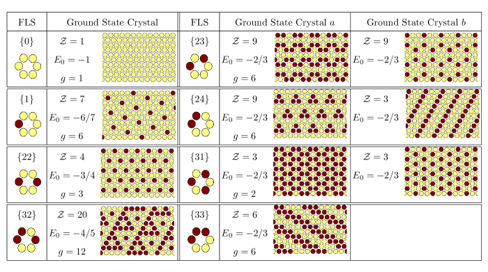
Figure 1: (Color online) The groundstates for the $8$ distinct FLS as defined in the text. The geometrical multiplicity $g$ of the FLS, number of sites in the unit cell $\mathcal{Z}$ and the energy per site $E_{0}$ in the groundstate are indicated. For the $\{23\}$, $\{24\}$ and $\{31\}$ FLS’s we find two degenerate polymorphs.

We have previously ronceray_short identified the ground states (all crystalline) for each choice of FLS. To assist the discussion of the various freezing transitions, we present the crystal phases for the different FLS’s in Figure 1 along with the energy per site $E_{o}$ and the number $g$ of distinct realizations of a FLS on the lattice. Note that three FLS’s have two distinct crystals with the same energy.

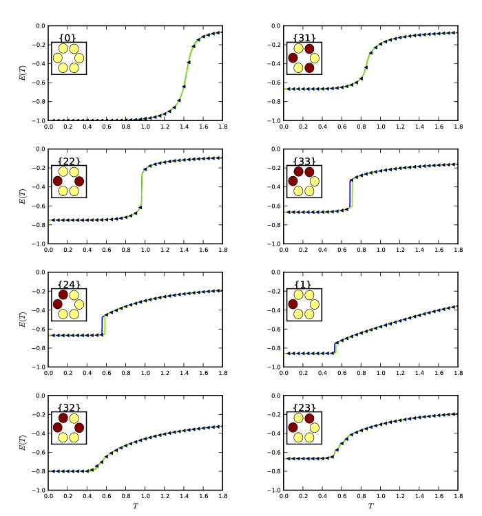
Figure 2: (Color online) The average energy per site as a function of temperature for each FLS. The measurements were made in an hysteresis cycle of temperature – cooling, in blue (dark gray) then heating, in green (light gray). These curves were obtained with a $60\times 60$ lattice and a “cooling rate” of $2.10^{6}$ steps of the rejection-free algorithm per site and per unit of temperature.

III Crystal-Liquid Phase Transitions

The temperature dependence of the average energies on heating and cooling are plotted in Figure 2 for each FLS. We note that the choice of FLS can result in either first order transitions ($\{1\}$, $\{24\}$ and $\{33\}$), continuous transitions ($\{0\}$, $\{22\}$ and $\{31\}$), or, in the case of $\{32\}$ and $\{23\}$, multiple transitions (see Figure 6 for a magnified view in this case). In the cases where two degenerate polymorphs exist we find that only one of the two is observed to form in the case of $\{23\}$ and $\{24\}$. The observed crystal is labeled $a$ in Figure 1. In the case of $\{31\}$, the polymorphs are spin-inversion symmetric and either can form spontaneously from the liquid.

In addition to the variety of freezing transitions, the equilibrium liquid states exhibit a considerable variation in their heat capacities $C_{V}=\frac{dE}{dT}$ and the maximum concentration of FLS that the liquid can accumulate before freezing. In a previous paper ronceray_liq we demonstrated that the influence of the choice of FLS on the liquid structure could be attributed to the difference in the entropy cost per FLS. Contributions to this entropy cost per FLS were found to come from both the symmetry of the favoured local structure itself (the higher the symmetry, the greater the entropy cost) and from the entropy of aggregates of FLS’s.

Not only does the decrease in symmetry of the FLS allow the liquid to accumulate more local order before freezing, but it also tends to result in large unit cells in the crystal ronceray_short . This coincidence of effects means that large unit cells in the crystal phase will often be associated with a liquid that can accumulate a significant amount of local structure (i.e. ’pre-order’) before freezing and help explain why we see little difference in the rate of crystallization of the different systems, even though the unit cell varies across a factor of 20. To appreciate the extent of this pre-ordering, consider the case of the $\{32\}$ FLS which freezes into our most complicated crystal structure (see Figure 1). This freezing involves multiple transitions (as we shall describe below) but if we select $T=0.6$, a temperature that lies just above the first of the ordering transitions, we find that the local ordering has already reached roughly $75\%$ of the final crystal order. In Figure 3 we show an example configuration in the $\{32\}$ liquid at $T=0.6$ in which the entangled fragments of the crystalline order are evident.

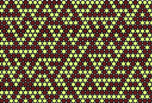
Figure 3: (Color online) Typical equilibrium spin configuration of the system for FLS $\{32\}$, at temperature $T=0.6$, just above the first transition. The extensive local structuring of the liquid appears clearly.

IV The Common Tangent Construction on the Entropy-Energy Plane

Two phases are in coexistence when their free energies are equal. Under the fixed size and temperature conditions of our simulations, the appropriate free energy is the canonical or Helmholtz free energy $F(T)=E(T)-TS(T)$ and the freezing point $T_{f}$ is identified through the resulting relation between the average energy $E(T)$ and the entropy $S(T)$,

$$E_{\mathrm{crystal}}(T_{f})-T_{f}S_{\mathrm{crystal}}(T_{f})=E_{\mathrm{liquid}}(T_{f})-T_{f}S_{\mathrm{liquid}}(T_{f})$$ (1)

For freezing transitions, a useful representation of the coexistence condition is a common tangent construction on the entropy-energy plane. This construction follows directly from Eq. 1 and the relation

$$dS(T)=\frac{1}{T}dE(T)$$ (2)

This relation between canonical quantities resembles the relation by which temperature is defined in the microcanonical ensemble, i.e. $\frac{1}{T}\equiv\frac{\partial S}{\partial E}$. Eq. 2 can be derived using the total differential $dF=dE-SdT-TdS$ combined with the classical relation $S=-\frac{\partial F}{\partial T}$ in the canonical ensemble.

Using Eq. 2, we can calculate the entropy $S(T)$ by integrating $1/T$ over the energy, i.e.

$$S(T)=S(T_{i})+\int_{E_{i}}^{E(T)}\frac{dE^{\prime}}{T(E^{\prime})}$$ (3)

where $T(E)$ is the temperature associated to the average energy $E(T)$ in Figure 2 and $T_{i}$ is the temperature at which $E(T_{i})=E_{i}$. To carry out this calculation we need to know the value of the entropy $S(T_{i})$ . For the liquid we choose the high temperature limit as our reference state. At $T\rightarrow\infty$, the entropy per spin is $S_{\infty}=\ln(2)$ (the factor $2$ reflecting the $2$ possible states of any individual site) and the energy is the average concentration of FLS’s in a random state of the system, i.e.

$$E_{\infty}=-\frac{g}{2^{6}}$$ (4)

where $g$ is the degeneracy of the FLS and is provided in Figure 1. The quantity $S_{\infty}$ corresponds to the total size of the configuration space and so is independent of the choice of FLS. $E_{\infty}$, as given by Eq.  4, does depend on the FLS via the multiplicity $g$, That said, we note that $E_{\infty}$ is small in magnitude and, as we shall see, this dependence contributes little to the overall influence of the choice of FLS on the thermodynamics. For the crystal, the ground state energy $E_{0}$ (also provided in Figure 1) provides the reference energy with an entropy $S(T=0)=0$.

Using Eq. 3 and the respective references states for the liquid and solid, we have calculated the liquid and solid entropies by numerical integration of the simulation data (in order to represent correctly the high temperature liquid, we used a regular sampling in the variable $1/T$ in this limit). In Figure 4 we plot the entropy $S(T)$ against the energy $E(T)$ for the different choices of FLS. As described above, the coexistence temperature $T_{f}$ is equal to the inverse of the slope of the common tangent between the solid and liquid entropy curves for those FLS’s that exhibit a 1st order freezing transition. These common tangents are indicated in each case by a straight dashed line. We have constructed this common tangent with the help of fitted curves for the entropy (power law at low temperature, polynomial for the liquid part), which serve only to get rid of the noise for the numerical construction of the tangent. This construction provides a precise estimate of the transition temperature, even when hysteresis phenomena prevent us from reading it directly on the $E(T)$ curve.

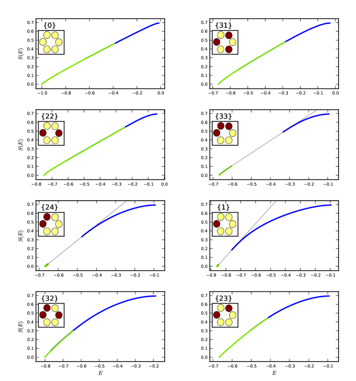
Figure 4: (Color online) The entropy $S(E)$ for the crystal (green / light gray) and liquid (blue / dark gray) for each choice of the FLS. The common tangent is indicated as a thin black line in the case of first order transitions.

For continuous transitions, both Eq. 1 and the equivalent common tangent construction in the $S$-$E$ plane are inadequate since there is no entropy nor energy difference between the two phases at the transition. For these transitions, we determined the transition temperature as the position of the peak in the heat capacity. The values of $T_{f}$ for each of the choices of FLS obtained either from the heat capacity peak or via the common tangent construction are presented in Table 1.

	Continuous			First order			Multi-step
FLS	{ 0 }	{ 31 }	{ 22 }	{ 33 }	{ 24 }	{ 1 }	{ 32 }	{ 23 }
$T_{f}$	1.43	0.85	0.96	0.70	0.57	0.54	0.34	0.53
							0.50	0.57
							0.56	0.64

Table 1: The freezing points of the various FLS systems. In the case of a continuous transition $T_{f}$ is determined as the position of the maximum of the heat capacity. In the case of a first order transition, $T_{f}$ is identified as the midpoint between the transition temperatures on heating and cooling. In case of multiple transitions, all the individual transition temperatures are presented.

The representation of the freezing transition in the $S$-$E$ plane allows for the most transparent connection to be made between the immediate consequences of the choice of FLS and the transition temperature. To illustrate this connection, we shall consider the following simple treatment. Let the liquid entropy be approximated by:

$$S(T)=S_{\infty}-A(E_{\infty}-E(T))^{2}$$ (5)

As explained in the Appendix, Eq. 5 represents the first term in an expansion of the liquid in terms of $(E_{\infty}-E)$ and the constant $A$ can be evaluated exactly for this expansion. These calculated values of $A$ are provided in ref. ronceray_liq . The second assumption is to assume that the crystal entropy at coexistence is zero. This assumption is justified by the observation on Figure 4 that the entropy range for the crystal is indeed very small as compared to the liquid’s. A more accurate treatment of the crystal entropy is provided by a single excitation model discussed in the Appendix. With these two assumptions, the common tangent construction is expressed by the relation

$$2A(E_{\infty}-E)=\frac{S_{\infty}-A(E_{\infty}-E)^{2}}{E-E_{o}}$$ (6)

Solving for $E$, the value of the liquid energy at coexistence, we have

$$E=E_{o}+\sqrt{\Delta^{2}-S_{\infty}/A}$$ (7)

where $\Delta=E_{\infty}-E_{o}$. The theoretical estimate of the transition temperature $T_{f}^{\mathrm{theory}}$, given by the inverse slope of the common tangent, is

$$T_{f}^{\mathrm{theory}}=\frac{1}{2A(\Delta-\sqrt{\Delta^{2}-S_{\infty}/A})}$$ (8)

As is evident from Eqs. 7 and 8, the freezing transition is determined (within this approximate treatment) by just two parameters: the crystal lattice energy, $E_{\infty}-E_{o}$, and the liquid entropy factor $A$. (The high temperature properties $S_{\infty}$ and $E_{\infty}$ being independent of FLS or approximately so, respectively.) The factor $A$ contains the entropy cost of structure in the liquid : a large value of $A$, generally associated with a high symmetry FLS, corresponds to a local structure that incurs a large entropy cost. In Fig. 5 we plot the values of $T_{f}^{\mathrm{theory}}$ calculated using Eq. 8 with the values of the freezing temperature from Table 1. Given the simplicity of the treatment, the theoretical estimates of the freezing temperatures are quite reasonable. The notable exception to this success is the FLS $\{1\}$ where the theory considerably overestimates transition temperature. The $\{1\}$ liquid actually exhibits a substantial decrease in energy prior to freezing, which is not correctly taken into account by the factor $A$, as previously noticed ronceray_liq , which explains this deviation. While this approximate treatment is too simple to establish whether a transition is first- or second-order, we note that it does appear to get the magnitude of the transition temperature roughly right, even for continuous transitions.

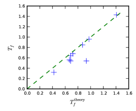
Figure 5: A scatter plot of the values of $T_{f}$ from simulation against the value of $T_{f}^{\mathrm{theory}}$ from Eq. 8. The straight line with slope one indicates the case where $T_{f}=T_{f}^{\mathrm{theory}}$.

V Freezing in Multiple Steps

The presence of multiple transitions for the $\{23\}$ and $\{32\}$ FLS’s is clearly seen when we examine the $E(T)$ curves with an expanded temperature scale about the transition region, as shown in Figure 6. In both cases, the freezing transition is made up of three distinct transitions. This is unusual for crystallization which is typically viewed as the archetype of a highly cooperative transition and hence unlikely to decouple in this way. In this Section we shall try to identify the intermediate phases associated with the step-wise freezing processes.

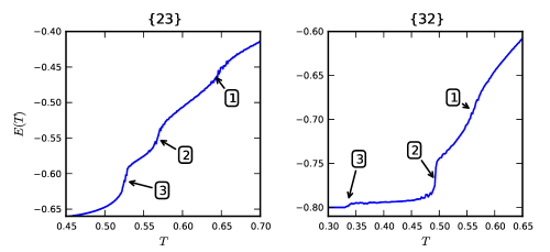
Figure 6: Energy versus temperature curve for multiple transitions systems. The positions of the individual transitions are indicated.

In the case of the $\{23\}$ FLS, the multiple transition scenario appears to arise from the existence of the two degenerate polymorphs (see Figure 1). If we identify the three transition temperature as $T_{1}$, $T_{2}$ and $T_{3}$, as indicated on Figure 6, it appears that the transition on cooling through $T_{2}$ corresponds to the formation of a polycrystalline mixture of the two polymorphs. Further cooling sees the formation at $T_{3}$ of the single phase of the preferred crystal phase. The nature of the continuous transition at $T_{1}$ remains a puzzle.

Turning to the transitions in the $\{32\}$ system , the picture is quite different. Instead of different crystal forms, the sequence of transitions correspond to a step-by-step symmetry breaking. Transition 1 marks the appearance of an orientation, at which the symmetry of the liquid is reduced from “isotropic” to a liquid with 3-fold rotational symmetry. On cooling, transition 2 is characterised by the loss of this rotational symmetry as a unique orientation is selected. Finally, transition 3 breaks the reflection symmetry and the translational invariance in one direction, to give the low $T$ crystalline state. Transitions 2 and 3 seem to be first order, though the small energy gap at transition 3 permits oscillation between phases in our finite size systems. This sequence of symmetry breakings is reminiscent of the liquid-nematic-smectic sequence of transitions observed in some molecular liquids.

VI Discussion

In the case of a single FLS, the choice of the stable structure determines the freezing transition temperature by determining the energy of the crystal lattice and the entropy cost of the FLS in the liquid. How might this picture change when we shift our focus to model liquids in which variations of the particle interactions are used to alter the local favoured structure? Previous work on modifications of the inter-particle potential for tetrahedral particles provides some insight into how subtle this problem can be. In the study by Molinero et al sastry on the modified silicon potential, increasing the strength of the 3-body bending force constant results in an increase in the temperature at which the liquid freezes into the diamond structure. Since the bending force constant has little effect on the solid, the influence of the potential acts through the liquid. An analysis of the enthalpy data sastry-supp for the modified silicon liquid indicates that the major effect of the increase in the bending constant is to increase the liquid enthalpy, an effect absent from the FLS model. In a model of spheres with a tetrahedral arrangement of sticky patches, the angular width $\sigma$ (in radians) of the individual patch represents another parameter for controlling the flexibility of the local structure. Doye et al doye have found that this model fails to crystallize at all, arguing that, for patch sizes down to 0.2 radians, there are multiple near degenerate structures - dodecahedral clusters, cubic diamond and hexagonal diamond - with the result being some sort of structural ’traffic jam’. In neither example cited here has the modification of the inter-particle potential corresponded to a change in the local geometry.

VII Conclusion

In this paper we have examined the variety of freezing transitions exhibited by a model liquid characterised by a favoured local structure. We found examples of ordering transitions that were first order, continuous and multi-stepped. All liquids were found to order with little or, in the case of the continuous transitions, no evidence of a tendency to supercool, in spite of the involvement of some complex crystal phases. The variation of the transition temperature with choice of favoured local structure was found to be reasonably captured by a simple expression involving the groundstate energy $E_{o}$ and the factor $A$ related to the entropy cost per FLS in the liquid.

A couple of observations follow directly from the results reported here. i) As all choices of FLS, with the exception of $\{0\}$, are frustrated (i.e. not all sites can lie simultaneously in the FLS : $E_{o}>-1$), it is clear that frustration provides no inherent impediment to freezing and is generally insufficient to stabilize the supercooled liquid. The competition between two FLS’s: one that can produce a low energy crystal while the other FLS, although more stable, can only order in a higher energy structure, looks like the simplest means of generating a glass forming liquid. ii) The intuitive notion that large unit cell crystals are more ’difficult’ to crystallize finds little support here. We note that the very feature (i.e low symmetry of the FLS) that results in large unit cells also ensures that the liquid, prior to freezing, can accumulate a substantial amount of the favoured local structure. As we have seen, these two effects tend to counter one another in setting the value of the transition temperature.

The FLS model provides a useful tool for building up our intuition on how local structure influences the properties of condensed matter. A report on the extension to 3D is currently in preparation ronceray-fcc . By building the model around the idea of local stable structures, rather than having to discover them as a consequence of particle interactions, we believe that the FLS approach offers a clearer language with which to ask questions about structure in condensed phases - both the influence of local structure and the nature of global ordering.

Acknowledgements

We gratefully acknowledge funding from the École Normale Supérieure and the Australian Research Council.

APPENDIX

In this Appendix we describe an alternative to the numerical fits used for the common tangent construction, which gives analytic values of the Taylor expansion coefficients around asymptotic high- and low-temperature regimes. We formerly derive the first order term of the expansion ronceray_liq . Here we generalize these results to any order using correlation functions that can be computed by exact enumeration. We also present a route to approximate the thermodynamic quantities at low temperature, though only to leading order.

VII.1 The Energy of the Low Temperature Crystal

We shall treat the energy of the crystal phase using a low temperature approximation in which we only include the (uncorrelated) single spin excitations from the groundstate. First, we identify the energy spectrum $(n_{i},\varepsilon_{i})$ of the ground state, as introduced in Table 7 in the example of system $\{22\}$. It classifies the single-spin defects that can occur in the crystal according to the energy of the corresponding state $\varepsilon_{i}$ and the proportion of site that can host such a defect $n_{i}$.

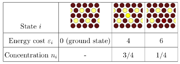
Figure 7: (Color online) Sketch of the energy spectrum of system $\{22\}$ at low temperature. For this system, two kinds of elementary (single spin) defects can occur in the crystal, examples of which are presented schematically (the ground state is also reminded). The energy spectrum of a crystal is determined by the energy costs $\varepsilon_{i}$ of each kind of defect, and the respective concentration of sites that can host such a defect $n_{i}$.

In the canonical ensemble at temperature $T$, each site of type $i$ has a probability:

$$p_{i}(T)=\frac{e^{-\varepsilon_{i}/T}}{1+e^{-\varepsilon_{i}/T}}$$

to be in its excited state, if we negligate the interaction between such defects. This gives the following approximate expression for the energy :

$$E(T)=E_{0}+\sum_{i}\varepsilon_{i}n_{i}\frac{e^{-\varepsilon_{i}/T}}{1+e^{-\varepsilon_{i}/T}}$$ (9)

All other thermodynamic quantities derive from $E(T)$. However the computation of $S(T)$, for example, involves complicated analytic forms, and it is much easier to compute it by numerical integration of Eq.9 using Eq. 3, to arbitrary precision.

A quantitative comparison between the results of simulations and this model is presented on Figure 8, for system $\{22\}$. We find that the accordance is quantitative up to a temperature around $T=0.6$. For the other systems, no qualitative difference was observed, though the quantitative values in the energy spectrum vary. This simple model gives a satisfying description of the crystal state, the physics of which is therefore quite simple. This method gives easily the leading order of the low-temperature expansion. Finding the corrections to this expansion would involve correlation between defects. No difficulty is expected to arise from that, though the computations would be rather tedious.

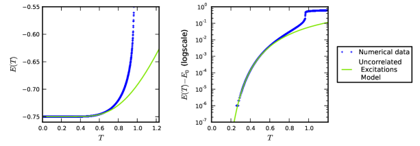
Figure 8: (Color online) The low temperature model described in equation 9, compared to simulated results for system $\{22\}$. The agreement is excellent at low temperature, as can be seen on the right figure, which is $E(T)-E_{0}$ plotted in logarithmic scale. This model correctly identifies leading-order behaviour at low temperature.

VII.2 Exact high-temperature expansion of the FLS model at all orders

In this section, we present an adapted version of the classical high-temperature expansions of spin models adapted to the FLS model. It gives the exact values of the coefficients of the Taylor expansion of the thermodynamic functions around $\beta=1/T=0$. These coefficients are connected correlation functions at infinite temperature, which may be computed exactly. This reasoning is an extension of our work in ronceray_liq , where we presented the route to compute the first non-trivial coefficient.

VII.2.1 Definitions :

To make the link with other spin models, we first introduce the Hamiltonian (energy of a configuration) :

$$H(\mathcal{C})=\sum_{i\in\Lambda}\epsilon_{i}$$ (10)

where $\Lambda$ is the lattice, $\mathcal{C}$ the spin configuration, and the local energy variables are :

$$\epsilon_{i}=\begin{cases}-1&\text{ if $i$ is in the FLS in configuration }\mathcal{C}\\ 0&\text{otherwise}\end{cases}$$ (11)

Each site of the lattice has $z$ neighbours ($z$ is the coordinence of the lattice). We assume invariance under translations, which impose to use periodic boundary conditions if the system is of finite size. For the triangular lattice studied here $z=6$. Note that the FLS model could be adapted to other regular lattices ; a review of this model on the 3D FCC lattice is in preparation.

The partition function of the system is defined as :

$$\mathcal{Z}(\beta)=\sum_{\mathcal{C}}\exp(-\beta H(\mathcal{C}))$$ (12)

where $\beta=1/T$ is the inverse temperature. All thermodynamic quantities derive from $\mathcal{Z}$ and its derivatives ; for example :

$$F(\beta)= -\frac{1}{\beta}\log\mathcal{Z}(\beta)$$ (13)

$$E(\beta)= -\frac{1}{\mathcal{Z}(\beta)}\frac{\partial\mathcal{Z}(\beta)}{\partial\beta}$$ (14)

$$S(\beta)= \beta(E-F)$$ (15)

are respectively the free energy, the average energy and the entropy of the system.

We define an average $\langle\cdot\rangle_{0}$ as the uniform average over all configurations, i.e. at $\beta=0$.

Note that for any site $i$, we have :

$$\langle\epsilon_{i}\rangle_{0}=E_{\infty}=-\frac{g}{2^{z}}$$ (16)

where $g$ is the degeneracy of the FLS and $E_{\infty}$ is the average energy per site at infinite temperature.

VII.2.2 Derivation

Now that the notations are set, we are ready to derive an exact Taylor expansion, at any order, of the thermodynamic functions in the FLS model around $\beta=0$.

Working on the partition function $\mathcal{Z}(\beta)$, a few usual tricks allow us to rewrite:

$$\mathcal{Z}(\beta) =\sum_{\mathcal{C}}\exp(-\beta H(\mathcal{C}))$$ (17)

$$=\sum_{\mathcal{C}}\prod_{i\in\Lambda}\exp(\beta\epsilon_{i})$$ (18)

$$=\sum_{\mathcal{C}}\prod_{i\in\Lambda}(1+\nu\epsilon_{i})$$ (19)

with $\nu=e^{\beta}-1$. Note that $\nu\approx\beta$ at high temperature. These simplifications use the fact that $\epsilon_{i}$ takes only two values, $0$ and $1$.

Now we can expand this product exactly :

$$\prod_{i\in\Lambda}(1+\nu\epsilon_{i})=\sum_{A\subseteq\Lambda}\nu^{|A|}\prod_{i\in A}\epsilon_{i}$$ (20)

The meaning of this expansion is the following : $A$ is the subset of right-side factors selected in the expansion of the product, and $|A|$ is the cardinal of $A$. If we now sum over configurations $\mathcal{C}$ :

$$\mathcal{Z}(\beta)= \sum_{\mathcal{C}}\prod_{i\in\Lambda}(1+\nu\epsilon_{i})$$ (21)

$$= 2^{N}\sum_{A\subseteq\Lambda}\nu^{|A|}\langle\prod_{i\in A}\epsilon_{i}\rangle_{0}$$ (22)

where $N$ is the total number of sites. We can rearrange this sum according to $|A|$ :

$$\mathcal{Z}(\beta)=2^{N}\sum_{k\in\mathbf{N}}\sum_{A\subseteq\Lambda,\ |A|=k}\nu^{k}\langle\prod_{i\in A}\epsilon_{i}\rangle_{0}$$ (23)

So finally we get the high temperature explicit, exact expansion :

$$\boxed{\mathcal{Z}(\beta)=2^{N}\sum_{k\in\mathbf{N}}\ \ \sum_{i_{1}\neq\dots\neq i_{k}}\nu^{k}\langle\epsilon_{i_{1}}\epsilon_{i_{2}}\dots\epsilon_{i_{k}}\rangle_{0}}$$ (24)

A convenient rewriting of this equation in terms of the free energy leads us to introduce the connected correlation functions:

$$\boxed{\beta F(\beta)=-\log\mathcal{Z}(\beta)=-N\log(2)-\sum_{k>0}\ \ \sum_{i_{1}\neq\dots\neq i_{k}}\nu^{k}\langle\epsilon_{i_{1}}\epsilon_{i_{2}}\dots\epsilon_{i_{k}}\rangle_{0}^{C}}$$ (25)

where :

$$\langle\epsilon_{i}\rangle_{0}^{C} =\langle\epsilon_{i}\rangle_{0}$$

$$\langle\epsilon_{i}\epsilon_{j}\rangle_{0}^{C} =\langle\epsilon_{i}\epsilon_{j}\rangle_{0}-\langle\epsilon_{i}\rangle_{0}\langle\epsilon_{j}\rangle_{0}$$

$$\langle\epsilon_{i}\epsilon_{j}\epsilon_{k}\rangle_{0}^{C} =\langle\epsilon_{i}\epsilon_{j}\epsilon_{k}\rangle_{0}-\langle\epsilon_{i}\rangle_{0}\langle\epsilon_{j}\epsilon_{k}\rangle_{0}-\langle\epsilon_{j}\rangle_{0}\langle\epsilon_{i}\epsilon_{k}\rangle_{0}-\langle\epsilon_{k}\rangle_{0}\langle\epsilon_{i}\epsilon_{j}\rangle_{0}+2\langle\epsilon_{i}\rangle_{0}\langle\epsilon_{j}\rangle_{0}\langle\epsilon_{k}\rangle_{0}$$

$$\dots$$

For the explicit computation, free energy representation is more convenient since connected correlation functions vanish as soon as a site is “far” (not overlapping) from the others. Thus every term in the expansion is extensive in the size of the system. In order to compute explicitly the connected correlation function at order $k$, we need to enumerate all possible ways to put an FLS in each of the $k$ sites $i_{1}\dots i_{k}$. It will be zero if they can be separated in two non-overlapping set of structures, thus we need only to enumerate a finite number of positions $i_{1}\dots i_{k}$. The quantity $\langle\epsilon_{i_{1}}\epsilon_{i_{2}}\dots\epsilon_{i_{k}}\rangle_{0}$ can be interpreted simply as the probability that all sites $i_{1}\dots i_{k}$ lie simultaneously in the FLS, in a random spin configuration.

VII.2.3 Computation of the first terms

The first terms read :

$$\beta F(\beta)=-N\log(2)-\nu\sum_{i\in\Lambda}\langle\epsilon_{i}\rangle_{0}^{C}+\nu^{2}\sum_{i\neq j}\langle\epsilon_{i}\epsilon_{j}\rangle_{0}^{C}+\nu^{3}\sum_{i\neq j\neq k}\langle\epsilon_{i}\epsilon_{j}\epsilon_{k}\rangle_{0}^{C}+O(\nu^{4})$$ (26)

The truncature to the order $\nu^{2}$ would give the Gaussian approximation to the density of states, as in ronceray_liq . Now the interest of this new, more formal approach, is to be able to increase the precision and involve higher-order correlation functions.

All that is left is to compute explicitly these connected correlation functions, which need only to test a finite (but possibly big) number of configurations. This is the only model-specific part of this derivation. Using enumerating routines, we could quite easily get the $\nu^{3}$ term for FCC and triangular lattices. Finally, to obtain an expansion of the free energy in powers of $\beta$ instead of $\nu$, we can substitute the expansion of $\nu$ in terms of $\beta$, i.e.

$$\nu=e^{\beta}-1=\sum_{k>0}\frac{\beta^{k}}{k!}=\beta+\beta^{2}/2+\beta^{3}/6+\dots$$ (27)

into Eq. 26.

References

- (1) F. C. Frank, Proc. Roy. Soc. A215, 43 (1952).
- (2) G. Tarjus, S. A. Kivelson, Z. Nussinov and P. Viot, J. Phys.: Cond. Matt. 17, R1143 (2005).
- (3) P. Ronceray and P. Harrowell, Europhys. Lett. 96, 30065 (2011). (2011).
- (4) P. Ronceray and P. Harrowell, J. Chem. Phys. 136, 134504 (2012).
- (5) M. Dzugutov, Phys. Rev. A 46, R2984 (1992).
- (6) M. Dzugutov, Phys. Rev. Lett. 70, 2924 (1993).
- (7) J. Roth and A.R.Denton, Phys. Rev. E 61, 6845 (2000).
- (8) F. Wooten abd D. Weaire, Solid State Phys. 40, 1 (1987).
- (9) V. Molinero and E. B. Moore, J. Phys. Chem. B 113, 4008 (2009).
- (10) F. H. Stillinger and T. A. Weber,Phys. Rev. B 31 5262 (1985).
- (11) V. Molinero, S. Sastry and C. A. Angell, Phys. Rev. Lett. 97, 075701 (2006).
- (12) F. Li, D. P. Josephson and A. Stein, Angew. Chem. Int. Ed. 50, 360 (2011).
- (13) D. Soloveichik and E. Winfree, Siam J. Comput. 36, 1544 (2007).
- (14) S. Hormoz and M. P. Brenner, Proc. Nat. Acad. Sci. USA 108, 5193 (2011).
- (15) S. H. Tindemans and B. M. Mulder, Phys. Rev. E 82, 021404 (2010).
- (16) A. W. Wilber, J. P.K. Doye and A. A. Louis, J. Chem. Phys. 131, 175101 (2009).
- (17) E. Bianchi, R. Blaak and C. N. Likos, Phys. Chem. Chem. Phys. 13, 6397 (2011).
- (18) P. Ronceray and P. Harrowell, in preparation.
- (19) A. B. Bortz, M. H. Kalos, and J. L. Lebowitz, J. Comp. Phys. 17, 10 (1975).
- (20) P. Ronceray and P. Harrowell, in preparation.
- (21) Supplimentary Material for V. Molinero, S. Sastry and C. A. Angell, Phys. Rev. Lett. 97, 075701 (2006).
- (22) J. K. P. Doye et. al., Phys. Chem. Chem. Phys. 9, 2197 (2007).