Improving the Hadron Physics of Non-Standard-Model Decays: Example Bounds on R-parity Violation

Abstract

Using the example of selected decays driven by R-parity-violating supersymmetric operators, we demonstrate how strong final-state interactions can be controlled quantitatively with high precision, thus allowing for a more accurate extraction of effective parameters from data. In our examples we focus on the lepton-flavor-violating decays $\tau\to\mu\pi^{+}\pi^{-}$. In R-parity violation these can arise due to the product of two couplings. We find bounds that are an order of magnitude stronger than previous ones.

1 Introduction

If weak-scale supersymmetry Nilles:1983ge is the solution to the hierarchy problem there must be new supersymmetric particles with masses below $\mathcal{O}(5\,\mathrm{TeV})$, which are accessible to the LHC. There are basically two forms of the minimal supersymmetric Standard Model, with light supersymmetric fields, distinguished by their superpotential. The most widely studied case is R-parity conservation, where the symmetries of the supersymmetric Standard Model are extended to include the discrete multiplicative symmetry R-parity. This renders the proton stable in the theory and the resulting renormalizable superpotential is given by

$$W_{\mathrm{MSSM}}=\epsilon_{ab}\left[(h_{e})_{ij}L_{i}^{a}H_{d}^{b}\bar{E}_{j}+(h_{d})_{ij}Q_{i}^{a}H_{d}^{b}\bar{D}_{j}+(h_{u})_{ij}Q_{i}^{a}H_{u}^{b}\bar{U}_{j}+\mu H_{d}^{a}H_{u}^{b}\right]\,.$$ (1)

Here $L,\,Q,H_{d},\,H_{u}$ are the lepton, quark, and Higgs SU(2)_L doublet left chiral superfields, respectively. $\bar{E},\,\bar{D},\,\bar{U}$ are the corresponding SU(2)_L singlet lepton and quark left chiral superfields. $i,j,k\in\{1,2,3\}$ are generation indices and $a,\,b\in\{1,2\}$ are SU(2)_L gauge indices. The $h_{f=e,d,u}$ are dimensionless Yukawa couplings and $\mu$ is the Higgs mass mixing term. Note that if non-renormalizable terms are allowed then for example the R-parity conserving superpotential term $QQQL$ leads to a dimension-five proton decay operator Nilles:1983ge . This is thus only suppressed by one power of the large mass scale. In this case proton hexality Dreiner:2005rd ; Dreiner:2003yr is the appropriate symmetry. It leads to the same low-energy superpotential given in Eq. (1), but prohibits all dimension-five proton decay operators.

Alternatively, the proton is also stable for the discrete $\mathbb{Z}_{3}$ symmetry baryon triality Ibanez:1991pr . The resulting renormalizable superpotential is Dreiner:1997uz

$$W_{\mathrm{B}_{3}}=W_{\mathrm{MSSM}}+\epsilon_{ab}\left[\lambda_{ijk}L_{i}^{a}L_{j}^{b}\bar{E}_{k}+\lambda^{\prime}_{ijk}L_{i}^{a}Q_{j}^{b}\bar{D}_{k}+\kappa_{i}L_{i}^{a}H_{u}^{b}\right]\,.$$ (2)

Here the $\lambda_{ijk},\,\lambda^{\prime}_{ijk}$ are dimensionless couplings and the $\kappa_{i}$ have dimension mass. Both baryon triality and proton hexality are discrete gauge anomaly-free in the sense of Refs. Dreiner:2005rd ; Ibanez:1991pr ; Krauss:1988zc . At any given energy scale the $\kappa_{i}$ can be rotated to zero, by a transformation in $(L_{i},\,H_{d})$ space Hall:1983id ; Dreiner:2003hw . Since we perform our computations at a fixed low-energy scale, we shall focus on the case $\kappa_{i}=0$ in the following.

An important feature of the additional terms in Eq. (2) is that they violate lepton number and flavor. Correspondingly there is a large set of bounds on the couplings $\lambda_{ijk}$ and $\lambda^{\prime}_{ijk}$. This was first considered in Ref. Hall:1983id , including also possible contributions to rare meson decays. A more systematic approach was taken in Ref. Barger:1989rk , considering bounds on all couplings individually. Since then many bounds have been set from the decays of mesons, including also bounds on products of operators Bhattacharyya:1995pq ; Agashe:1995qm ; Bhattacharyya:1995cg ; Altarelli:1997ce ; Dreiner:1997cd ; Kim:1997rr ; Allanach:1999ic ; herbi02 ; herbi07 . In Ref. Barger:1989rk , for example, the authors considered the R-parity-violating contributions to

$$R_{\pi}\equiv\frac{\Gamma(\pi\to e\nu)}{\Gamma(\pi\to\mu\nu)}\,.$$ (3)

An operator $\lambda^{\prime}_{21k}L_{2}Q_{1}\bar{D}_{k}$ contributes only to ${\Gamma(\pi\to\mu\nu)}$, thus modifying $R_{\pi}$. In computing the exact contribution to ${\Gamma(\pi\to\mu\nu)}$, one uses the definition

$$\langle 0|\bar{u}\gamma^{\mu}P_{L}d|\pi^{-}(q)\rangle\equiv-\frac{i}{\sqrt{2}}\,f_{\pi}q^{\mu}$$ (4)

of the pion decay constant $f_{\pi}$ for the $V-A$ current, and the current-algebra approximation

$$\langle 0|\bar{u}P_{L}d|\pi^{-}(q)\rangle=\sqrt{2}i\,\frac{M_{\pi}^{2}}{m_{u}+m_{d}}f_{\pi}$$ (5)

for the chiral (pseudo)scalar coupling. Here, $M_{\pi}$ denotes the charged pion mass, $m_{u,d}$ are the first-generation quark masses, and we make use of the left- and right-handed projection operators $P_{L/R}=(1\mp\gamma_{5})/2$. Using the experimental value including the error of $R_{\pi}$ PDG , which agrees with the Standard Model, results in a bound on $\lambda^{\prime}_{21k}$. This assumes that $L_{2}Q_{1}\bar{D}_{k}$ is the sole new operator contributing.

More recently Herrero and collaborators have studied $\tau$ decays in various R-parity conserving supersymmetric models Arganda:2008jj ; herrero09 , for example the decays

$$\tau^{\pm}\rightarrow\mu^{\pm}+f_{0}\,/\,\pi^{+}\pi^{-},\,\pi^{0}\pi^{0}\,/\,K^{+}K^{-},\,K^{0}\bar{K}^{0}\,/\,\eta,\,\eta^{\prime}\,/\,\rho^{0},\,\phi~{}.$$ (6)

The authors go beyond the simple current algebra approximation and employ chiral perturbation theory and resonance chiral theory resChPT . They thus dramatically improve the precision of the computation and therefore also the resulting bounds on new physics. The purpose of this paper is to refine these techniques further—in particular, we include both the scalar form factors and the vector form factor, model-independently. In addition, we will also discuss the case of R-parity violation. Specifically we shall focus on the decay

$$\tau^{\pm}\rightarrow\mu^{\pm}\pi^{+}\pi^{-}$$ (7)

to clarify our method. In terms of R-parity-violating operators, this decay receives contributions via the parton level processes

$$\tau^{\pm}\rightarrow\mu^{\pm}u_{i}\bar{u}_{k}\qquad\mathrm{and}\qquad\tau^{\pm}\rightarrow\mu^{\pm}d_{j}\bar{d}_{k}~{}.$$ (8)

Combining the operators $\epsilon_{ab}\lambda_{ijk}L_{i}^{a}L_{j}^{b}\bar{E}_{k}$ and $\epsilon_{ab}\lambda^{\prime}_{ijk}L_{i}^{a}Q_{j}^{b}\bar{D}_{k}$ from the superpotential in Eq. (2) and integrating out the heavy intermediate scalar fermion, we obtain several independent contributions to the decay $\tau^{-}\to\mu^{-}+2$ quarks (cf. Appendix A):

1. Combining $\epsilon_{ab}\lambda^{\prime}_{3ij}L_{3}^{a}Q_{i}^{b}\bar{D}_{j}$ and $[\epsilon_{ab}\lambda^{\prime}_{2kj}L_{2}^{a}Q_{k}^{b}\bar{D}_{j}]^{\dagger}$ corresponds to $\tau^{-}\to\mu^{-}\bar{u}_{i}u_{k}$ with

   $$\mathscr{L}_{\mathrm{eff}}=\frac{1}{2}\frac{\lambda^{\prime}_{3ij}\lambda^{\prime*}_{2kj}}{m^{2}_{\tilde{d}_{j}}}(\bar{u}_{k}\gamma^{\alpha}P_{L}u_{i})(\bar{\mu}\gamma_{\alpha}P_{L}\tau)~{}.$$ (9)

2. Combining $\epsilon_{ab}\lambda^{\prime}_{3ij}L_{3}^{a}Q_{i}^{b}\bar{D}_{j}$ and $\left[\epsilon_{ab}\lambda^{\prime}_{2i\ell}L_{2}^{a}Q_{i}^{b}\bar{D}_{\ell}\right]^{\dagger}$ corresponds to $\tau^{-}\to\mu^{-}d_{j}\bar{d}_{\ell}$ with

   $$\mathscr{L}_{\mathrm{eff}}=\frac{1}{2}\frac{\lambda^{\prime}_{3ij}\lambda^{\prime*}_{2i\ell}}{m^{2}_{\tilde{u}_{i}}}(\bar{d}_{j}\gamma^{\alpha}P_{R}d_{\ell})(\bar{\mu}\gamma_{\alpha}P_{L}\tau)~{}.$$ (10)

3. Combining $\epsilon_{ab}\lambda_{3i2}L_{3}^{a}L_{i}^{b}\bar{E}_{2}$ and $[\epsilon_{ab}\lambda^{\prime}_{ijk}L_{i}^{a}Q_{j}^{b}\bar{D}_{k}]^{\dagger}$ corresponds to $\tau^{-}\to\mu^{-}d_{j}\bar{d}_{k}$ with

   $$\mathscr{L}_{\mathrm{eff}}=\frac{1}{2}\frac{\lambda_{3i2}\lambda^{\prime*}_{ijk}}{m^{2}_{\tilde{\nu}_{i}}}(\bar{d}_{j}P_{R}d_{k})(\bar{\mu}P_{L}\tau)~{}.$$ (11)

   Figure 1: Feynman diagrams inducing transitions of the type $\tau^{-}\to\mu^{-}\bar{u}u$ (a) or $\tau^{-}\to\mu^{-}\bar{d}d$ (b)–(d) by exchange of supersymmetric particles. The arrows denote the direction of the flow of the left-handed fields. The particle labels denote the incoming ($\tau^{-}$) or outgoing fields (all others). Thus in (b), e.g., we have an outgoing (SU(2) singlet) $d_{j}$ and (SU(2) singlet) $\bar{d}_{\ell}$.

4. Combining $\epsilon_{ab}\lambda_{2i3}L_{2}^{a}L_{i}^{b}\bar{E}_{3}$ and $[\epsilon_{ab}\lambda^{\prime}_{ijk}L_{i}^{a}Q_{j}^{b}\bar{D}_{k}]^{\dagger}$ corresponds to $\tau^{-}\to\mu^{-}\bar{d}_{j}d_{k}$ with

   $$\mathscr{L}_{\mathrm{eff}}=\frac{1}{2}\frac{\lambda_{2i3}\lambda^{\prime*}_{ijk}}{m^{2}_{\tilde{\nu}_{i}}}(\bar{d}_{k}P_{L}d_{j})(\bar{\mu}P_{R}\tau)~{}.$$ (12)

Diagrammatic representations of contributions (a)–(d) are shown in Fig. 1.

2 Application to the vector current

The invariant mass distribution of the width for the decay $\tau\to\mu\pi^{+}\pi^{-}$ is given by

$$\frac{d\Gamma}{d\sqrt{s}}=\frac{1}{(2\pi)^{5}}\frac{1}{16m_{\tau}^{2}}\,{\overline{\left|\mathcal{M}\right|^{2}}}|\mathbf{p}_{\pi^{+}}^{\,*}|d\Omega_{+}^{*}\,|{\mathbf{p}}_{\mu}|d\Omega_{\mu}\ ,$$ (13)

where $s$ is the invariant mass squared of the pion pair, $|{\mathbf{p}}_{\pi^{+}}^{\,*}|$ ($\Omega_{\pi^{+}}^{*}$) is the momentum (angle) of the ${\pi^{+}}$ in the rest frame of the pion pair, and $|{\mathbf{p}}_{\mu}|$ and $\Omega_{\mu}$ are to be given in the $\tau$ rest frame.

The essential observation is that the matrix element $\mathcal{M}$ factorizes, since the primary transition is short-ranged (the range of interaction is set by the inverse mass of the exchanged supersymmetric particles), while the final-state interaction is long-ranged. Therefore, we may write

$$\mathcal{M}=\big{\langle}\pi^{+}\pi^{-}\big{|}\hat{O}^{(\alpha)}\big{|}0\big{\rangle}M^{r}_{(\alpha)}\ .$$ (14)

The reduced matrix elements $M^{r}_{(\alpha)}$ are to be calculated in the underlying, fundamental theory, while the hadronic matrix elements $\big{\langle}\pi^{+}\pi^{-}\big{|}\hat{O}^{(\alpha)}\big{|}0\big{\rangle}$ can be deduced either from data or determined with theoretical input.

To begin with, let us assume that only the vector current contributes here—the generalization to the scalar current is straightforward and will be presented below. As long as isospin is assumed to be conserved, two pions with vector quantum numbers (i.e., in a $P$-wave) only couple to the isovector component of the current. Therefore we need to consider only a single form factor and the hadronic matrix element is given by the pion vector form factor, $F_{V}(s)$, defined via

$$\big{\langle}\pi^{+}(p_{\pi^{+}})\pi^{-}(p_{\pi^{-}})\big{|}\tfrac{1}{2}(\bar{u}\gamma^{\alpha}u-\bar{d}\gamma^{\alpha}d)\big{|}0\big{\rangle}\equiv F_{V}(s)(p_{\pi^{+}}-p_{\pi^{-}})^{\alpha}\ .$$ (15)

$F_{V}(s)$ is very well known both from direct measurements of $e^{+}e^{-}\to\pi^{+}\pi^{-}$ Na7FF ; KLOE-1 ; CMD2-1 ; CMD2-2 ; babarFF ; KLOE-2 and, via an isospin rotation, of $\tau^{-}\to\pi^{-}\pi^{0}\nu_{\tau}$ BelleFF , as well as theoretical studies Gasser:1990bv ; guerrero ; Oller ; yndurain ; Anant . It collects all non-perturbative $\pi\pi$ interactions and is universal in the elastic region, which to excellent approximation comprises the energy range $s<1$ GeV².

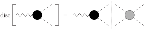
Figure 2: Graphical representation of the discontinuity relation for the pion form factor. The dashed lines are pions, while the wavy line stands for the current coupling to these. The black disc denotes the form factor, while the gray disc denotes the pion–pion scattering $T$-matrix (which, by angular momentum conservation, is automatically projected onto the appropriate partial wave).

We briefly illustrate how to describe $F_{V}(s)$ theoretically, based solely on the fundamental principles of analyticity and unitarity. Figure 2 gives a graphical illustration of the discontinuity of the form factor, regarded as an analytic function of $s$ in the complex plane cut along (parts of) the positive real axis, in the elastic regime, i.e., considering two-pion intermediate states only. It is given by

$$\text{disc}\,F_{V}(s) =F_{V}(s+i\epsilon)-F_{V}(s-i\epsilon)=2i\,\text{Im}\,F_{V}(s)$$

$$=2i\,F_{V}(s)\,\sigma(s)\,t_{1}^{1}(s)^{*}\,\theta\big{(}s-4M_{\pi}^{2}\big{)}=2i\,F_{V}(s)\sin\delta_{1}^{1}(s)e^{-i\delta_{1}^{1}(s)}\,\theta\big{(}s-4M_{\pi}^{2}\big{)}\,,$$ (16)

where $\sigma(s)=\sqrt{1-4M_{\pi}^{2}/s}$ is proportional to the two-particle phase space, and $t_{\ell}^{I}(s)$ refers to the pion–pion partial-wave amplitude of isospin $I$ and angular momentum $\ell$, obtained from expanding the corresponding $T$-matrix in Legendre polynomials. In the final step, we have rewritten the $P$-wave amplitude in terms of the phase shift $\delta_{1}^{1}(s)$ in the canonical manner. One immediately deduces Watson’s final-state theorem watson : reality of $\text{Im}\,F_{V}(s)$ implies that the phase of $F_{V}(s)$ coincides with $\delta_{1}^{1}(s)$. The solution to Eq. (16) is given by

$$F_{V}(s)=P_{V}(s)\Omega_{1}^{1}(s)~{},\quad\Omega_{1}^{1}(s)=\exp\bigg{\{}\frac{s}{\pi}\int_{4M_{\pi}^{2}}^{\infty}ds^{\prime}\frac{\delta_{1}^{1}(s^{\prime})}{s^{\prime}(s^{\prime}-s)}\bigg{\}}~{},$$ (17)

where $\Omega_{1}^{1}(s)$ is the Omnès function Omnes and $P_{V}(s)$ a polynomial. The pion–pion phase shifts are known to excellent precision (up to at least $\sqrt{s}\simeq 1.1$ GeV) from analyses of the highly constrained system of dispersion relations known as Roy equations Roy ; ACGL ; CCL ; garcia .

Perturbative QCD suggests $F_{V}(s)$ should fall off like $1/s$ for large values of $s$ (up to logarithmic corrections) BrodskyLepage , which is also the behavior of the Omnès function if the phase shift approaches $\pi$ asymptotically, as phenomenology indeed suggests. Hence, $P_{V}(s)$ is required to be a constant. Gauge invariance finally requires the normalization to be fixed to $F_{V}(s=0)=1$, therefore $P_{V}(s)\equiv 1$. The representation Eq. (17) can be improved by taking inelastic effects (beyond two-pion intermediate states) into account. We here use a parametrization presented in Ref. FFnew , which describes the available high-precision data Na7FF ; KLOE-1 ; CMD2-1 ; CMD2-2 ; babarFF ; KLOE-2 ; BelleFF perfectly.

The relevant reduced matrix elements needed to complete Eq. (14)—read off from the effective Lagrangians given in Eqs. (9)–(12)—can be subsumed in the expression

$$M^{r}_{V\alpha}=\lambda_{V}\left[\bar{\mu}(p_{\mu})\gamma_{\alpha}P_{L}\tau(p_{\tau})\right]\ ,$$ (18)

where the effective coupling $\lambda_{V}$ is given by

$$\lambda_{V}\equiv\frac{1}{4}\bigg{(}\frac{\lambda^{\prime}_{31j}\lambda^{\prime*}_{21j}}{m_{\tilde{d}_{j}}^{2}}-\frac{\lambda^{\prime}_{3i1}\lambda^{\prime*}_{2i1}}{m_{\tilde{u}_{i}}^{2}}\bigg{)}~{}.$$ (19)

This in principle comprises six different contributions ($i,j=1,2,3$) which can enhance each other or lead to cancellations, depending on the phases of the R-parity-violating couplings. In the Standard Model there is a strong hierarchy among the Yukawa couplings. For example the top quark Yukawa coupling is almost a factor of forty larger than the bottom quark Yukawa coupling. Since no supersymmetry with or without R-parity has yet been found, we shall for simplicity consider one product of operators at a time in Eq. (19). We thus employ the assumption that there is a hierarchy in the unknown R-parity-violating couplings Barger:1989rk ; Dreiner:1991pe .

Using Eqs. (15) and (18) in the definition of the matrix element we find for the spin-averaged squared matrix element

$$\frac{1}{2}\sum_{\rm spins}|\mathcal{M}|^{2}=\frac{\lambda_{V}^{2}}{2}\big{(}s-4M_{\pi}^{2}\big{)}\bigg{[}m_{\tau}^{2}+m_{\mu}^{2}-s+\frac{\lambda(m_{\tau}^{2},m_{\mu}^{2},s)}{s}z^{2}\bigg{]}\big{|}F_{V}(s)\big{|}^{2}~{},$$ (20)

where we included a prefactor of 1/2 from averaging the incoming $\tau$ polarizations. $\lambda(x,y,z)=x^{2}+y^{2}+z^{2}-2(xy+xz+yz)$ is the usual Källén function, and $z=\cos\theta$ denotes the angle of the pions relative to the leptons in the $\pi\pi$ rest frame. Evaluating the angular integral and collecting all kinematic prefactors, we arrive at

$$\frac{d\Gamma_{V}}{d\sqrt{s}}=\frac{\lambda_{V}^{2}}{256\pi^{3}m_{\tau}^{3}}\big{(}s-4M_{\pi}^{2}\big{)}^{3/2}\lambda^{1/2}\big{(}m_{\tau}^{2},m_{\mu}^{2},s\big{)}\bigg{[}m_{\tau}^{2}+m_{\mu}^{2}-s+\frac{\lambda(m_{\tau}^{2},m_{\mu}^{2},s)}{3s}\bigg{]}\big{|}F_{V}(s)\big{|}^{2}\ .$$ (21)

Since all quantities but $\lambda_{V}$ are known in Eq. (21), it provides the kind of expression we are looking for. In particular, the norm of the hadronic current is fixed unambiguously in contrast to previous studies, where quark-model wave functions were employed to fix the normalization.

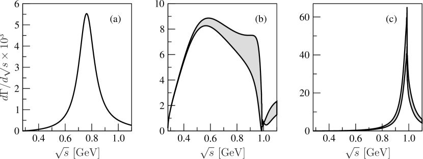
Figure 3: The predicted signals individually for the currents (a) $\bar{q}\gamma^{\alpha}q$, (b) $(\bar{u}u+\bar{d}d)/2$, and (c) $\bar{s}s$. In all cases the effective coupling constant is set to 1 GeV^-2. For the uncertainty bands of the scalar form factors, see the discussion in the main text.

The resulting $\sqrt{s}$ distribution is depicted in panel (a) of Fig. 3, where we have used $\lambda_{V}=1$ GeV^-2, which is easily rescaled.

The signal in the vector channel can be represented reasonably well by a Breit–Wigner distribution with an energy-dependent width as provided by various parametrizations. Here the advantage of our approach lies mainly in its fixed normalization—we briefly compare to the narrow-resonance approximation (where one studies the decay $\tau\to\mu\,\rho^{0}(770)$, assuming a stable $\rho^{0}$) in Appendix B. An additional advantage is that not only the modulus of the form factor, but also its phase is fixed unambiguously, such that the interference of various currents can be analyzed as well.

3 Application to the scalar currents

Contrary to the vector currents, scalar currents are typically not well represented by Breit–Wigner functions (for a detailed discussion see e.g. Ref. Gardner:2001gc ). In this case, isospin symmetry requires two pions to couple exclusively to isoscalar scalar currents. However, there are two such form factors, originating from non-strange and strange isoscalar scalar sources. They are called $\Gamma_{\pi}^{n}$ and $\Gamma_{\pi}^{s}$, respectively, and will contribute simultaneously. The use of scalar form factors (as opposed to Breit–Wigner parametrizations) is unavoidable if one wants to determine the underlying couplings in a controlled way.

The expressions analogous to Eq. (15) now read

$$\left\langle\pi^{+}\pi^{-}\left|\bar{q}q\right|0\right\rangle\equiv\mathcal{B}^{q}\Gamma_{\pi}^{q}(s)\ ,$$ (22)

where the quark flavors may be either $\bar{q}q=(\bar{u}u+\bar{d}d)/2$ for the light quarks, with the superscript $q=n$ denoting the corresponding scalar form factor, or $\bar{q}q=\bar{s}s$ for strange quarks (with superscript $q=s$). Furthermore, $\mathcal{B}^{n}=M_{\pi}^{2}/(m_{u}+m_{d})$, $\mathcal{B}^{s}=(2M_{K}^{2}-M_{\pi}^{2})/(2m_{s})$. With this convention, the form factors, $\Gamma^{q}_{\pi}(s)$, are invariant under the QCD renormalization group. For the numerical evaluation, we will use the values obtained from averaging lattice computations with $N_{f}=2+1$ dynamical flavors FLAG , $(m_{u}+m_{d})/2=(3.43\pm 0.11)\,$MeV, $m_{s}=(94\pm 3)\,$MeV, to be understood in the $\overline{\rm MS}$ scheme at the running QCD scale $\mu=2\,$GeV. In addition, in analogy to Eq. (18) we may now write

$$M_{S}^{q\,r}=\lambda_{S}^{q}\left[\bar{\mu}(p_{\mu})P_{R}\tau(p_{\tau})\right]\ ,$$ (23)

where, again, the superscript $q$ denotes the quark flavor fed by the corresponding operator. Comparison to Eqs. (11) and (12) yields

$$\lambda_{S}^{n}\equiv\frac{(\lambda_{3i2}+\lambda_{2i3})\lambda^{\prime*}_{i11}}{4m^{2}_{\tilde{\nu}_{i}}}~{},\quad\lambda_{S}^{s}\equiv\frac{(\lambda_{3i2}+\lambda_{2i3})\lambda^{\prime*}_{i22}}{4m^{2}_{\tilde{\nu}_{i}}}~{}.$$ (24)

With these expressions we find

$$\frac{d\Gamma_{S}}{d\sqrt{s}}=\frac{1}{64\pi^{3}m_{\tau}^{3}}\big{(}s-4M_{\pi}^{2}\big{)}^{1/2}\lambda^{1/2}\big{(}m_{\tau}^{2},m_{\mu}^{2},s\big{)}\Big{[}(m_{\tau}+m_{\mu})^{2}-s\Big{]}\big{|}\mathcal{B}^{n}\lambda_{S}^{n}\Gamma_{\pi}^{n}(s)+\mathcal{B}^{s}\lambda_{S}^{s}\Gamma_{\pi}^{s}(s)\big{|}^{2}\,.$$ (25)

Experimentally, the scalar form factors are not accessible as directly and unambiguously as the vector form factor. However, they can be reconstructed from dispersion theory, similar to what we discussed as the Omnès representation of the vector form factor in the previous section. The main difference is that the elastic approximation breaks down much earlier in the pion–pion $S$-wave (of isospin $I=0$) due to the strong inelastic coupling of two $S$-wave pions to $K\bar{K}$ in the region of the $f_{0}(980)$, i.e., beginning immediately at the $K\bar{K}$ threshold. In order to describe the scalar form factors including energies around the mass of the $f_{0}(980)$, it is therefore mandatory to solve a two-channel Muskhelishvili–Omnès problem Omnes ; Muskhelishvili . The discontinuity equation (16) has to be generalized to two coupled channels for the scalar form factors of pion and kaon. The two-channel $T$-matrix correspondingly can be parametrized in terms of three input functions, the pion–pion $S$-wave phase shift $\delta_{0}^{0}(s)$ known from Roy equation solutions ACGL ; CCL ; garcia , as well as modulus and phase of the inelastic reaction $\pi\pi\to K\bar{K}$ Cohen ; Etkin ; BDM04 . We again assume the fall-off of all scalar form factors $\propto 1/s$, and the scattering phases involved to approach integer multiples of $\pi$ in the appropriate way. The solution to the coupled-channel discontinuity equation cannot be written down analytically in a similarly compact form as for the single-channel case, Eq. (17), but has to be constructed numerically DGL90 ; Moussallam99 ; Descotes ; HDKM . It now depends on the constant normalization of the corresponding pion and kaon form factors $\Gamma_{\pi/K}^{n/s}(s=0)$. In contrast to the vector case, the normalizations of the scalar form factors are not fixed by symmetries; they are however related to the corresponding masses by the Feynman–Hellmann theorem Hellmann ; Feynman ,

$$\Gamma_{\pi}^{n}(0)=\frac{1}{2\mathcal{B}^{n}}\bigg{(}\frac{\partial}{\partial m_{u}}+\frac{\partial}{\partial m_{d}}\bigg{)}M_{\pi}^{2}~{},\quad\Gamma_{\pi}^{s}(0)=\frac{1}{\mathcal{B}^{s}}\frac{\partial}{\partial m_{s}}M_{\pi}^{2}~{},$$ (26)

and similar for the scalar form factors of the kaon. At leading order in the quark mass expansion, one therefore has $\Gamma_{\pi}^{n}(0)=1$, $\Gamma_{\pi}^{s}(0)=0$, $\Gamma_{K}^{n}(0)=1/2$, and $\Gamma_{K}^{s}(0)=1$. Beyond that, information on these quantities can again be deduced from lattice calculations. We vary the normalizations of the kaon form factors according to $\Gamma_{K}^{n}(0)=0.4\ldots 0.6$, $\Gamma_{K}^{s}(0)=0.95\ldots 1.15$, as suggested by the uncertainties in the corresponding low-energy constants given in Ref. FLAG , while keeping the rather well-known pion-form-factor normalizations fixed at $\Gamma_{\pi}^{n}(0)=0.98$, $\Gamma_{\pi}^{s}(0)=0$.

In Figs. 3(b) and (c) we show the resulting invariant mass distributions for the pion pair for $(\lambda_{S}^{q}=1$ GeV^-2, $\lambda_{S}^{s}=0$) and $(\lambda_{S}^{q}=0$, $\lambda_{S}^{s}=1$ GeV^-2), respectively, with the uncertainty bands as dictated by the above estimates for the uncertainty in the kaon form factor normalizations. In panel $(b)$ the $f_{0}(500)$ (or $\sigma$ meson) shows up as a broad bump with a clear non-Breit–Wigner shape, while the $f_{0}(980)$ produces a peak exclusively in the strangeness form factor, panel $(c)$. Thus, were a pronounced peak just below 1 GeV observed in $\tau\to\mu\pi^{+}\pi^{-}$, it would allow one to straightforwardly extract $\lambda_{S}^{s}$ from data, without the need to employ any assumption on the internal structure of the $f_{0}(980)$—additional information can be gained from also studying the $\bar{K}K$ final state, which however we will not detail here. This highlights the advantage of our approach compared to the one of Ref. herrero09 : in that work assumptions on the quark content of the $f_{0}(980)$ need to be employed in order to derive bounds, which then in turn strongly depend on these assumptions. In our case the bounds can be deduced directly from a fit to the spectra, once they are measured.

4 Discussion

If supersymmetry was to show up in experiments like $\tau\to\mu\pi^{+}\pi^{-}$, there is no a priori reason why pion pairs in the vector channel would be significantly more populated than pion pairs in the scalar channel. While the effective couplings for the vector channel are given by squark exchange, the scalar channel is driven by sneutrino-exchange contributions. Thus one should expect interferences of the three currents discussed individually above. In this context it is important to stress that, below the first significant inelastic threshold, the phase of the form factor agrees with that of the elastic scattering amplitude watson , which is well known in both the scalar and the vector channel ACGL ; CCL ; garcia .

The Belle collaboration has given upper limits on branching ratios $\mathcal{B}(\tau^{-}\to\mu^{-}\pi^{+}\pi^{-})$ with different kinematical cuts Miyazaki:2008mw ; Miyazaki:2011xe ; Miyazaki:2012mx . In particular, they find

$$\mathcal{B}\big{(}\tau^{-}\to\mu^{-}\rho^{0}(770)\big{)}\times\mathcal{B}\big{(}\rho^{0}(770)\to\pi^{+}\pi^{-}\big{)} <1.2\times 10^{-8}~{},$$

$$\mathcal{B}\big{(}\tau^{-}\to\mu^{-}f_{0}(980)\big{)}\times\mathcal{B}\big{(}f_{0}(980)\to\pi^{+}\pi^{-}\big{)} <3.4\times 10^{-8}~{},$$

$$\mathcal{B}\big{(}\tau^{-}\to\mu^{-}\pi^{+}\pi^{-}\big{)} <2.1\times 10^{-8}~{}.$$ (27)

The resonance signals are isolated by applying cuts to the $\pi^{+}\pi^{-}$ invariant mass spectrum, specifically $906\,{\rm MeV}<\sqrt{s}<1065\,{\rm MeV}$ for the $f_{0}(980)$ Miyazaki:2008mw and $587\,{\rm MeV}<\sqrt{s}<962\,{\rm MeV}$ for the $\rho(770)$ Miyazaki:2011xe . As we aim for deriving upper limits on coupling constants from null experiments, what will effectively enter the bounds on the scalar couplings are the lower limits of the uncertainty bands on the scalar form factors. Note that the vector form factor is known to a precision that any uncertainty therein is totally irrelevant at the accuracy we aim for. When comparing to the last, inclusive, bound in Eq. (27), we will set all form factors to zero above $1.1$ GeV where we deem our representations not very reliable anymore; obviously, the bounds could be improved upon if lower bounds were available also at higher energies. Integrating Eqs. (21) and (25) in the respective ranges, we find

$$\int_{587\,{\rm MeV}}^{962\,{\rm MeV}}\bigg{(}\frac{d\Gamma_{V}}{d\sqrt{s}} +\frac{d\Gamma_{S}}{d\sqrt{s}}\bigg{)}d\sqrt{s}=\Big{[}0.94|\lambda_{V}|^{2}+\{2.3\ldots 3.0\}|\lambda_{S}^{n}|^{2}+\{2.5\ldots 3.7\}\,\text{Re}\big{(}\lambda_{S}^{n}\lambda_{S}^{s*}\big{)}$$

$$+\{1.2\ldots 1.8\}|\lambda_{S}^{s}|^{2}\Big{]}\times 10^{-3}{\rm GeV}^{5}$$

$$<2.7\times 10^{-20}{\rm GeV}\ ,$$

$$\int_{906\,{\rm MeV}}^{1065\,{\rm MeV}}\bigg{(}\frac{d\Gamma_{V}}{d\sqrt{s}} +\frac{d\Gamma_{S}}{d\sqrt{s}}\bigg{)}d\sqrt{s}=\Big{[}0.10|\lambda_{V}|^{2}+\{0.3\ldots 0.6\}|\lambda_{S}^{n}|^{2}+\{0.5\ldots 2.1\}\,\text{Re}\big{(}\lambda_{S}^{n}\lambda_{S}^{s*}\big{)}$$

$$+\{0.35\ldots 0.42\}\,\text{Im}\big{(}\lambda_{S}^{n}\lambda_{S}^{s*}\big{)}+\{2.5\ldots 3.7\}|\lambda_{S}^{s}|^{2}\Big{]}\times 10^{-3}{\rm GeV}^{5}$$

$$<7.7\times 10^{-20}{\rm GeV}\ ,$$

$$\int_{2M_{\pi}}^{1100\,{\rm MeV}}\bigg{(}\frac{d\Gamma_{V}}{d\sqrt{s}} +\frac{d\Gamma_{S}}{d\sqrt{s}}\bigg{)}d\sqrt{s}=\Big{[}1.05|\lambda_{V}|^{2}+\{4.3\ldots 5.1\}|\lambda_{S}^{n}|^{2}+\{2.4\ldots 4.7\}\,\text{Re}\big{(}\lambda_{S}^{n}\lambda_{S}^{s*}\big{)}$$

$$+\{0.47\ldots 0.57\}\,\text{Im}\big{(}\lambda_{S}^{n}\lambda_{S}^{s*}\big{)}+\{3.2\ldots 4.7\}|\lambda_{S}^{s}|^{2}\Big{]}\times 10^{-3}{\rm GeV}^{5}$$

$$<4.8\times 10^{-20}{\rm GeV}\ ,$$ (28)

where the limits on the branching fractions have been converted into partial widths with the help of the lifetime of the $\tau$ lepton. The uncertainties shown for the coefficients of the scalar couplings are due to the ranges assumed for the kaon scalar form factor normalizations as discussed above. They are displayed explicitly in order to indicate the remaining potential for improvement, once this specific hadronic input is still better known. Note that contributions $\propto\text{Im}\big{(}\lambda_{S}^{n}\lambda_{S}^{s*}\big{)}$ have to come from above the $K\bar{K}$ threshold, where the two interfering scalar form factors are not required to have identical phases according to Watson’s theorem watson any more.

In order to set limits on the underlying coupling constants, we shall make the usual simplifying assumption that they are all real. Thus, assuming the first operator in Eq. (19) dominates we obtain for example the bound

$$\lambda_{21i}^{\prime*}\lambda_{31i}^{\prime}<2.1\cdot 10^{-4}\left(\frac{m_{\tilde{d}_{i}}}{100\,\mathrm{GeV}}\right)^{2}\,.$$ (29)

The corresponding bound on the second operator is

$$\lambda_{2i1}^{\prime*}\lambda_{3i1}^{\prime}<2.1\cdot 10^{-4}\left(\frac{m_{\tilde{u}_{i}}}{100\,\mathrm{GeV}}\right)^{2}\,.$$ (30)

A complete list is given in Table 1.

product of couplings	bound	susy mass	eff. coupling
$\lambda_{21i}^{\prime*}\lambda_{31i}^{\prime}$	$2.1\cdot 10^{-4}$	$m_{\tilde{d}_{i}}$	$\lambda_{V}$
$\lambda_{2i1}^{\prime*}\lambda_{3i1}^{\prime}$	$2.1\cdot 10^{-4}$	$m_{\tilde{u}_{i}}$	$\lambda_{V}$
$\lambda_{3i2}\lambda_{i11}^{\prime*}$, $\lambda_{2i3}\lambda_{i11}^{\prime*}$	$1.3\cdot 10^{-4}$	$m_{\tilde{\nu}_{i}}$	$\lambda_{S}^{n}$
$\lambda_{3i2}\lambda_{i22}^{\prime*}$, $\lambda_{2i3}\lambda_{i22}^{\prime*}$	$1.5\cdot 10^{-4}$	$m_{\tilde{\nu}_{i}}$	$\lambda_{S}^{s}$

Table 1: Our best bounds on the products of supersymmetric R-parity-violating couplings. We assume all other couplings to be zero. The bounds scale with the square of the given mass divided by 100 GeV, so for a 1 TeV mass they are a factor 100 weaker. To obtain the bound we employed the effective coupling in the far right column. Note that in the first two rows for the case of $i=1$ both operator products contribute in $\lambda_{V}$ and the relative phases are essential. They can only be treated separately if $m_{\tilde{d}_{1}}\ll m_{\tilde{u}_{1}}$ or $m_{\tilde{u}_{1}}\ll m_{\tilde{d}_{1}}$.

Note that while the most restrictive bound on the vector coupling $\lambda_{V}$ and the underlying products of fundamental coupling constants is derived from the dedicated search for $\tau^{-}\to\mu^{-}\rho^{0}(770)$ Miyazaki:2011xe , the best limits on the two effective scalar couplings stem from the most recent limit on $\tau^{-}\to\mu^{-}\pi^{+}\pi^{-}$ without further kinematical cuts Miyazaki:2012mx . In the literature the best previous bound is given from different processes bounding the individual couplings separately Allanach:1999ic . Combining them to a product bound we obtain

$$\lambda^{\prime}_{21i}\lambda^{\prime}_{31i}<7.2\cdot 10^{-3}\left(\frac{m_{\mathrm{susy}}}{100\,\mathrm{GeV}}\right)^{2}\,,$$ (31)

where we have set the mass of the different virtual supersymmetric scalars equal. We have thus improved this bound by more than a factor of 30. We can also compare our result to the related bounds obtained in Ref. Black:2002wh . The authors consider the effective operators

$$\mathcal{O}_{j}=\frac{C^{j}_{\alpha\beta}}{\Lambda^{2}}(\bar{\mu}\Gamma_{j}\tau)(\bar{q}^{\alpha}\Gamma_{j}q^{\beta})\,,$$ (32)

independent of their origin, for different Dirac structures $\Gamma_{j}$. These contribute for example to $\tau\to\mu\pi^{+}\pi^{-}$. Setting $C^{j}=4\pi$ the authors obtain the bounds

$$\Lambda>2.6\,\mathrm{TeV\;(scalar)},\quad\Lambda>12\,\mathrm{TeV\;(vector)}\,,$$ (33)

where ‘scalar’ and ‘vector’ denote the cases $\Gamma_{j}=\mathbf{1}$ and $\Gamma_{j}=\gamma^{\alpha}$, respectively. Comparing the vector case to our bound we thus have

$$\frac{\lambda^{\prime}_{21i}\lambda^{\prime}_{31i}}{4\tilde{m}^{2}}=\frac{4\pi}{\Lambda^{2}}\,,$$ (34)

hence

$$\lambda^{\prime}_{21i}\lambda^{\prime}_{31i}=16\pi\left(\frac{\tilde{m}}{\Lambda}\right)^{2}<3.5\cdot 10^{-3}\left(\frac{\tilde{m}}{100\,\mathrm{GeV}}\right)^{2}\,,$$ (35)

which is more than an order of magnitude weaker than our bound, partly owing to weaker experimental bounds at the time. We point out that in Ref. Black:2002wh the scalar form factors were assumed to be constant, which is, as we have discussed, not a good approximation.

5 Conclusions

Supersymmetry has to-date not been observed. Thus well-motivated versions, such as R-parity violation, which however have been considered less conventional, are now also being investigated in more detail. Most of the strictest bounds on supersymmetry with R-parity violation arise from precision, low-energy observables, e.g. meson decays, or decays involving mesons. These computations typically involve simple approximations of the relevant hadron physics, such as the current algebra approximation. In this paper we demonstrate that the bounds on the R-parity-violating couplings can be considerably improved when including dynamical aspects of hadron physics. We do this in a model-independent manner, such that it can easily be applied to test other fundamental theories of physics beyond the Standard Model.

To be specific, we have focused on the decay $\tau^{\pm}\to\mu^{\pm}\pi^{+}\pi^{-}$. Here, the hadron physics aspects can be treated particularly rigorously, as the strong final-state interactions of the pion pair are described in terms of the vector and scalar form factors, which are either directly measured experimentally, or can be reconstructed using the rigorous, model-independent methods of dispersion theory. We then employ upper bounds found by the Belle collaboration on the branching ratios of the lepton-flavor-violating $\tau$ decays, and obtain bounds on products of the R-parity-violating couplings. Due to the extra information we have included and the slightly improved experimental data we find bounds which are more than an order of magnitude stronger than previous ones.

Appendix A Derivation of effective operators

In this Appendix we present as an example the computation of the effective Lagrangian given in Eq. (9). We show the results in four-component spinor notation, as this still is the most widely used convention across communities. However, we actually derived the results in two-component spinor notation Dreiner:2008tw and then translated them into four-component notation using Appendix G of Ref. Dreiner:2008tw .

The superpotential in Eq. (2) contains the terms $\epsilon_{ab}\lambda_{ijk}^{\prime}L_{i}^{a}Q_{j}^{b}\bar{D}_{k}$. In component fields the corresponding Yukawa Lagrangian terms are given by, see for example Ref. Richardson:2000nt ,

$$\mathscr{L}_{\mathrm{LQD}}=-\lambda_{ijk}^{\prime}\Big{(} \tilde{d}^{*}_{kR}\overline{\nu^{c}_{i}}P_{L}d_{j}-\tilde{d}^{*}_{kR}\overline{\ell^{c}_{i}}P_{L}u_{j}+\tilde{d}_{jL}\bar{d}_{k}P_{L}\nu_{i}$$

$$-\tilde{u}_{jL}\bar{d}_{k}P_{L}\ell_{i}+\tilde{\nu}_{i}\bar{d}_{k}P_{L}d_{j}-\tilde{\ell}_{iL}\bar{d}_{k}P_{L}u_{j}+\mathrm{h.c.}\Big{)}\,,$$ (36)

where we have assumed that the Yukawa coupling is real and we have denoted the charged lepton by $\ell_{i}$. The charge conjugate field is defined as $\ell_{i}^{c}\equiv C{{\bar{\ell}_{i}}}^{T}$. If we now combine the second term for $i=3$ as well as the hermitian conjugate of the second term for $i=2$, identify the third index, and assume the intermediate $\tilde{d}_{k}$ squark to be very heavy, we obtain the effective Lagrangian

$$\mathscr{L_{\mathrm{eff}}}=-\frac{\lambda^{\prime}_{3ij}\lambda_{2kj}^{\prime*}}{m^{2}_{\tilde{d}_{j}}}\left(\overline{\tau^{c}}P_{L}u_{i}\right)\left(\bar{u}_{k}P_{R}\mu^{c}\right)~{}.$$ (37)

A Fierz reordering as well as employing the definition of the complex conjugate field then gives the form for the effective interaction in Eq. (9)

$$\mathscr{L}_{\mathrm{eff}}=\frac{1}{2}\frac{\lambda^{\prime}_{3ij}\lambda^{\prime*}_{2kj}}{m^{2}_{\tilde{d}_{j}}}(\bar{u}^{k}\gamma^{\alpha}P_{L}u^{i})(\bar{\mu}\gamma_{\alpha}P_{L}\tau)~{}.$$ (38)

Appendix B Comparison to the narrow-resonance approximation

In this Appendix, we briefly compare our treatment of the $\tau\to\mu\pi^{+}\pi^{-}$ decay in terms of form factors to the narrow-resonance approximation. If, e.g., the $\rho$ meson were a stable particle, instead of Eq. (14) we had to use, cf. Ref. herbi02 ; herbi07 ,

$$\mathcal{M}=\big{\langle}\rho(k)\big{|}\hat{J}^{\alpha}\big{|}0\big{\rangle}M^{r}_{V\,\alpha}\ ,\quad\big{\langle}\rho(k)\big{|}\hat{J}^{\alpha}\big{|}0\big{\rangle}=\big{\langle}\rho(k)\big{|}\tfrac{1}{2}(\bar{u}\gamma^{\alpha}u-\bar{d}\gamma^{\alpha}d)\big{|}0\big{\rangle}=\frac{1}{\sqrt{2}}f_{\rho}M_{\rho}\epsilon(\lambda)^{\alpha\ *}\ ,$$ (39)

where $f_{\rho}=220$ MeV denotes the $\rho$ decay constant and $\epsilon(\lambda)$ is the $\rho$ polarization vector. The expressions for the physical and the stable $\rho$ are most easily compared on the level of the decay rates. Employing the identity

$$\sum_{\lambda}\epsilon(\lambda)_{\alpha}^{*}\epsilon(\lambda)_{\beta}=-g_{\alpha\beta}+\frac{k_{\alpha}k_{\beta}}{M_{\rho}^{2}}\ ,$$ (40)

one finds that switching from a stable $\rho$ to an unstable one is obtained by the replacement

$$\frac{1}{2}f_{\rho}^{2}M_{\rho}^{2} \to-\frac{1}{3}(2\pi)^{3}\int ds\int d\Phi_{2}(q,p_{\pi^{+}},p_{\pi^{-}})({p}_{\pi^{+}}-{p}_{\pi^{-}})^{2}\left|F_{V}(s)\right|^{2}$$

$$=\frac{1}{6\pi^{2}}\int ds\Theta(s-4M_{\pi}^{2})\frac{|{\mathbf{p}}_{\pi^{+}}^{*}|^{3}}{\sqrt{s}}\left|F_{V}(s)\right|^{2}\ ,$$ (41)

where $q^{2}=s$, we use the definition of the phase space as given in Ref. PDG , and $({p}_{\pi^{+}}-{p}_{\pi^{-}})^{2}=-4{\mathbf{p}}_{\pi^{+}}^{\,*\ 2}$ in the center-of-mass frame. In order to understand under which circumstances the full expression is well represented by the left hand side of Eq. (41), we may parametrize the pion vector form factor by its spectral function, assuming a constant width. Then we may write

$$|F_{V}(s)|^{2}\simeq\frac{M_{\rho}^{4}}{(s-M_{\rho}^{2})^{2}+M_{\rho}^{2}\Gamma_{\rho}^{2}}=\pi\frac{M_{\rho}^{3}}{\Gamma_{\rho}}\rho(s)\ .$$ (42)

As a consequence of unitarity the spectral function is normalized,

$$\int_{4M_{\pi}^{2}}^{\infty}ds\,\rho(s)=1\ .$$ (43)

In experiments the $\rho$ meson is typically identified by imposing cuts on the two-pion invariant mass. If for the sake of the argument here we assume that these cuts were sufficiently wide that the normalization integral is exhausted, we find, using the explicit expression for the $\rho$ width

$$\Gamma_{\rho}=\frac{g_{\rho\pi\pi}^{2}}{6\pi}\frac{|{\mathbf{p}}_{\pi^{+}}^{*}|^{3}}{M_{\rho}^{2}}$$ (44)

as well as the KSFR relation $g_{\rho\pi\pi}^{2}=M_{\rho}^{2}/(2f_{\pi}^{2})$ KS ; FR ,

$$f_{\rho}=2f_{\pi}\ ,$$ (45)

which is a known connection e.g. in the hidden-local-symmetry approach HLS . With $f_{\pi}=92.2$ MeV, this identity is fulfilled to about 20% accuracy. However, in any realistic situation the $\rho$ meson in the final state can only be isolated by cuts on the $\pi\pi$ invariant mass, such that the $\rho$ spectral function is not fully saturated, leading to uncontrolled inaccuracies in the extraction of the effective parameters.

References

- (1) H. P. Nilles, Supersymmetry, Supergravity and Particle Physics, Phys. Rept. 110 (1984) 1.
- (2) H. K. Dreiner, C. Luhn and M. Thormeier, What is the discrete gauge symmetry of the MSSM?, Phys. Rev. D 73 (2006) 075007 [hep-ph/0512163].
- (3) H. K. Dreiner, H. Murayama and M. Thormeier, Anomalous flavor U(1)(X) for everything, Nucl. Phys. B 729 (2005) 278 [hep-ph/0312012].
- (4) L. E. Ibáñez and G. G. Ross, Discrete gauge symmetries and the origin of baryon and lepton number conservation in supersymmetric versions of the standard model, Nucl. Phys. B 368 (1992) 3.
- (5) B. C. Allanach, A. Dedes and H. K. Dreiner, R-parity-violating minimal supergravity model, Phys. Rev. D 69 (2004) 115002 [Erratum-ibid. D 72 (2005) 079902] [hep-ph/0309196].
- (6) L. M. Krauss and F. Wilczek, Discrete Gauge Symmetry in Continuum Theories, Phys. Rev. Lett. 62 (1989) 1221.
- (7) L. J. Hall and M. Suzuki, Explicit R-Parity Breaking in Supersymmetric Models, Nucl. Phys. B 231 (1984) 419.
- (8) H. K. Dreiner and M. Thormeier, Supersymmetric Froggatt–Nielsen models with baryon- and lepton-number violation, Phys. Rev. D 69 (2004) 053002 [hep-ph/0305270].
- (9) V. D. Barger, G. F. Giudice and T. Han, Some New Aspects of Supersymmetry R-Parity-Violating Interactions, Phys. Rev. D 40 (1989) 2987.
- (10) G. Bhattacharyya and D. Choudhury, and decays: Placing new bounds on R-parity-violating supersymmetric coupling, Mod. Phys. Lett. A 10 (1995) 1699 [hep-ph/9503263].
- (11) K. Agashe and M. Graesser, R-parity violation in flavor changing neutral current processes and top quark decays, Phys. Rev. D 54 (1996) 4445 [hep-ph/9510439].
- (12) G. Bhattacharyya and A. Raychaudhuri, Searching R-parity-violating supersymmetry in semileptonic decays, Phys. Lett. B 374 (1996) 93 [hep-ph/9512277].
- (13) G. Altarelli, J. R. Ellis, G. F. Giudice, S. Lola and M. L. Mangano, Pursuing interpretations of the HERA large data, Nucl. Phys. B 506 (1997) 3 [hep-ph/9703276].
- (14) H. K. Dreiner and P. Morawitz, High anomaly at HERA and supersymmetry, Nucl. Phys. B 503 (1997) 55 [hep-ph/9703279].
- (15) J. E. Kim, P. Ko and D.-G. Lee, More on R-parity- and lepton-family-number-violating couplings from muon(ium) conversion, and and decays, Phys. Rev. D 56 (1997) 100 [hep-ph/9701381].
- (16) B. C. Allanach, A. Dedes and H. K. Dreiner, Bounds on R-parity-violating couplings at the weak scale and at the GUT scale, Phys. Rev. D 60 (1999) 075014 [hep-ph/9906209].
- (17) H. K. Dreiner, G. Polesello and M. Thormeier, Bounds on broken R parity from leptonic meson decays, Phys. Rev. D 65 (2002) 115006 [hep-ph/0112228].
- (18) H. K. Dreiner, M. Kramer and B. O’Leary, Bounds on R-parity-violating supersymmetric couplings from leptonic and semi-leptonic meson decays, Phys. Rev. D 75 (2007) 114016 [hep-ph/0612278].
- (19) J. Beringer et al. [Particle Data Group], Review of Particle Physics, Phys. Rev. D 86 (2012) 010001.
- (20) E. Arganda, M. J. Herrero and J. Portolés, Lepton-flavour-violating semileptonic decays in constrained MSSM-seesaw scenarios, JHEP 0806 (2008) 079 [arXiv:0803.2039 [hep-ph]].
- (21) M. J. Herrero, J. Portolés and A. M. Rodríguez-Sánchez, Sensitivity to the Higgs Sector of SUSY-Seesaw Models in the Lepton-Flavour-Violating decay, Phys. Rev. D 80 (2009) 015023 [arXiv:0903.5151 [hep-ph]].
- (22) G. Ecker, J. Gasser, A. Pich and E. de Rafael, The Role of Resonances in Chiral Perturbation Theory, Nucl. Phys. B 321 (1989) 311.
- (23) S. R. Amendolia et al. [NA7 Collaboration], A Measurement of the Space-Like Pion Electromagnetic Form Factor, Nucl. Phys. B 277 (1986) 168.
- (24) A. Aloisio et al. [KLOE Collaboration], Measurement of and extraction of below 1 GeV with the KLOE detector, Phys. Lett. B 606 (2005) 12 [hep-ex/0407048].
- (25) R. R. Akhmetshin et al., Measurement of the cross section with the CMD-2 detector in the 370–520 MeV c.m. energy range, JETP Lett. 84 (2006) 413 [Pisma Zh. Eksp. Teor. Fiz. 84 (2006) 491] [hep-ex/0610016].
- (26) R. R. Akhmetshin et al. [CMD-2 Collaboration], High-statistics measurement of the pion form factor in the -meson energy range with the CMD-2 detector, Phys. Lett. B 648 (2007) 28 [hep-ex/0610021].
- (27) B. Aubert et al. [BABAR Collaboration], Precise measurement of the cross section with the Initial State Radiation method at BABAR, Phys. Rev. Lett. 103 (2009) 231801 [arXiv:0908.3589 [hep-ex]].
- (28) F. Ambrosio et al. [KLOE Collaboration], Measurement of from threshold to 0.85 GeV2 using Initial State Radiation with the KLOE detector, Phys. Lett. B 700 (2011) 102 [arXiv:1006.5313 [hep-ex]].
- (29) M. Fujikawa et al. [Belle Collaboration], High-Statistics Study of the Decay, Phys. Rev. D 78 (2008) 072006 [arXiv:0805.3773 [hep-ex]].
- (30) J. Gasser and U.-G. Meißner, Chiral expansion of pion form factors beyond one loop, Nucl. Phys. B 357 (1991) 90.
- (31) F. Guerrero and A. Pich, Effective field theory description of the pion form factor, Phys. Lett. B 412 (1997) 382 [hep-ph/9707347].
- (32) J. A. Oller, E. Oset and J. E. Palomar, Pion and kaon vector form factors, Phys. Rev. D 63 (2001) 114009 [hep-ph/0011096].
- (33) J. F. De Trocóniz and F. J. Ynduráin, Precision determination of the pion form factor and calculation of the muon , Phys. Rev. D 65 (2002) 093001 [hep-ph/0106025].
- (34) B. Ananthanarayan, I. Caprini and I. S. Imsong, Implications of the recent high statistics determination of the pion electromagnetic form factor in the timelike region, Phys. Rev. D 83 (2011) 096002 [arXiv:1102.3299 [hep-ph]].
- (35) F. Niecknig, B. Kubis and S. P. Schneider, Dispersive analysis of and decays, Eur. Phys. J. C 72 (2012) 2014 [arXiv:1203.2501 [hep-ph]].
- (36) K. M. Watson, Some general relations between the photoproduction and scattering of mesons, Phys. Rev. 95 (1954) 228.
- (37) R. Omnès, On the solution of certain singular integral equations of quantum field theory, Nuovo Cim. 8 (1958) 316.
- (38) S. M. Roy, Exact integral equation for pion–pion scattering involving only physical region partial waves, Phys. Lett. B 36 (1971) 353.
- (39) B. Ananthanarayan, G. Colangelo, J. Gasser and H. Leutwyler, Roy equation analysis of scattering, Phys. Rept. 353 (2001) 207 [hep-ph/0005297].
- (40) I. Caprini, G. Colangelo and H. Leutwyler, private communication.
- (41) R. García-Martín, R. Kamiński, J. R. Peláez, J. Ruiz de Elvira and F. J. Ynduráin, The Pion–pion scattering amplitude. IV: Improved analysis with once subtracted Roy-like equations up to 1100 MeV, Phys. Rev. D 83 (2011) 074004 [arXiv:1102.2183 [hep-ph]].
- (42) G. P. Lepage and S. J. Brodsky, Exclusive Processes in Perturbative Quantum Chromodynamics, Phys. Rev. D 22 (1980) 2157.
- (43) C. Hanhart, A New Parameterization for the Pion Vector Form Factor, Phys. Lett. B 715 (2012) 170 [arXiv:1203.6839 [hep-ph]].
- (44) H. K. Dreiner and G. G. Ross, R-parity violation at hadron colliders, Nucl. Phys. B 365 (1991) 597.
- (45) S. Gardner and U.-G. Meißner, Rescattering and chiral dynamics in decay, Phys. Rev. D 65 (2002) 094004 [hep-ph/0112281].
- (46) G. Colangelo et al., Review of lattice results concerning low energy particle physics, Eur. Phys. J. C 71, 1695 (2011) [arXiv:1011.4408 [hep-lat]].
- (47) N. I. Muskhelishvili, Singular Integral Equations, Wolters-Noordhoff Publishing, Groningen, 1953 [Dover Publications, 2nd edition, 2008].
- (48) D. H. Cohen, D. S. Ayres, R. Diebold, S. L. Kramer, A. J. Pawlicki and A. B. Wicklund, Amplitude Analysis of the System Produced in the Reactions and at 6 GeV/c, Phys. Rev. D 22 (1980) 2595.
- (49) A. Etkin et al., Amplitude Analysis of the System Produced in the Reaction at 23 GeV/c, Phys. Rev. D 25 (1982) 1786.
- (50) P. Büttiker, S. Descotes-Genon and B. Moussallam, A new analysis of scattering from Roy and Steiner type equations, Eur. Phys. J. C 33 (2004) 409 [arXiv:hep-ph/0310283].
- (51) J. F. Donoghue, J. Gasser and H. Leutwyler, The decay of a light Higgs boson, Nucl. Phys. B 343 (1990) 341.
- (52) B. Moussallam, dependence of the quark condensate from a chiral sum rule, Eur. Phys. J. C 14 (2000) 111 [hep-ph/9909292].
- (53) S. Descotes-Genon, Zweig rule violation in the scalar sector and values of low-energy constants, JHEP 0103 (2001) 002 [hep-ph/0012221].
- (54) M. Hoferichter, C. Ditsche, B. Kubis and U.-G. Meißner, Dispersive analysis of the scalar form factor of the nucleon, JHEP 1206 (2012) 063 [arXiv:1204.6251 [hep-ph]].
- (55) H. Hellmann, Einführung in die Quantenchemie, Franz Deuticke, Leipzig, 1937.
- (56) R. P. Feynman, Forces in Molecules, Phys. Rev. 56 (1939) 340.
- (57) V. Bernard, S. Descotes-Genon and G. Toucas, Topological susceptibility on the lattice and the three-flavour quark condensate, JHEP 1206 (2012) 051 [arXiv:1203.0508 [hep-ph]].
- (58) Y. Miyazaki et al. [Belle Collaboration], Search for Lepton-Flavor-Violating Decays into Lepton and Meson, Phys. Lett. B 672 (2009) 317 [arXiv:0810.3519 [hep-ex]].
- (59) Y. Miyazaki et al. [Belle Collaboration], Search for Lepton-Flavor-Violating Decays into a Lepton and a Vector Meson, Phys. Lett. B 699 (2011) 251 [arXiv:1101.0755 [hep-ex]].
- (60) Y. Miyazaki et al. [Belle Collaboration], Search for Lepton-Flavor-Violating and Lepton-Number-Violating Decay Modes, arXiv:1206.5595 [hep-ex].
- (61) D. Black, T. Han, H.-J. He and M. Sher, – flavor violation as a probe of the scale of new physics, Phys. Rev. D 66 (2002) 053002 [hep-ph/0206056].
- (62) H. K. Dreiner, H. E. Haber and S. P. Martin, Two-component spinor techniques and Feynman rules for quantum field theory and supersymmetry, Phys. Rept. 494 (2010) 1 [arXiv:0812.1594 [hep-ph]].
- (63) P. Richardson, Simulations of R-parity-violating SUSY models, hep-ph/0101105.
- (64) K. Kawarabayashi and M. Suzuki, Partially conserved axial vector current and the decays of vector mesons, Phys. Rev. Lett. 16 (1966) 255.
- (65) Riazuddin and Fayyazuddin, Algebra of current components and decay widths of and mesons, Phys. Rev. 147 (1966) 1071.
- (66) M. Harada and K. Yamawaki, Hidden local symmetry at loop: A New perspective of composite gauge boson and chiral phase transition, Phys. Rept. 381 (2003) 1 [hep-ph/0302103].