Cross-Correlation of SDSS DR7 Quasars and DR10 BOSS Galaxies: The Weak Luminosity Dependence of Quasar Clustering at $z\sim 0.5$

Abstract

We present the measurement of the two-point cross-correlation function (CCF) of $8,198$ Sloan Digital Sky Survey (SDSS) Data Release 7 (DR7) quasars and $349,608$ DR10 CMASS galaxies from the Baryonic Oscillation Spectroscopic Survey (BOSS) at redshift $\bar{z}\sim 0.5$ ($0.3<z<0.9$). The cross-correlation function can be reasonably well fit by a power-law model $\xi_{QG}(r)=(r/r_{0})^{-\gamma}$ on projected scales of $r_{p}=2-25\,h^{-1}{\rm Mpc}$ with $r_{0}=6.61\pm 0.25\,h^{-1}$Mpc and $\gamma=1.69\pm 0.07$. We estimate a quasar linear bias of $b_{Q}=1.38\pm 0.10$ at $\langle z\rangle=0.53$ from the CCF measurements. This linear bias corresponds to a characteristic host halo mass of $\sim 4\times 10^{12}\,h^{-1}M_{\odot}$, compared to $\sim 10^{13}\,h^{-1}M_{\odot}$ characteristic host halo mass for CMASS galaxies. Based on the clustering measurements, most quasars at $\bar{z}\sim 0.5$ are not the descendants of their higher luminosity counterparts at higher redshift, which would have evolved into more massive and more biased systems at low redshift. We divide the quasar sample in luminosity and constrain the luminosity dependence of quasar bias to be $db_{Q}/d\log L=0.20\pm 0.34$ or $0.11\pm 0.32$ (depending on different luminosity divisions) for quasar luminosities $-23.5>M_{i}(z=2)>-25.5$, implying a weak luminosity dependence of quasar clustering for the bright end of the quasar population at $\bar{z}\sim 0.5$. We compare our measurements with theoretical predictions, Halo Occupation Distribution (HOD) models and mock catalogs. These comparisons suggest quasars reside in a broad range of host halos, and the host halo mass distributions significantly overlap with each other for quasars at different luminosities, implying a poor correlation between halo mass and instantaneous quasar luminosity. We also find that the quasar HOD parameterization is largely degenerate such that different HODs can reproduce the CCF equally well, but with different outcomes such as the satellite fraction and host halo mass distribution. These results highlight the limitations and ambiguities in modeling the distribution of quasars with the standard HOD approach and the need for additional information in populating quasars in dark matter halos with HOD.

I. introduction

Quasars are powered by mass accretion onto supermassive black holes (SMBHs) at the center of massive galaxies. Like galaxies, quasars are luminous tracers of the underlying dark matter, and can be used to map the large-scale structure of the Universe. Over the past decade, quasar clustering has been measured for large statistical samples drawn from dedicated surveys, most notably the Sloan Digital Sky Survey (SDSS, York et al., 2000) and the 2dF QSO Redshift Survey (2QZ, Croom et al., 2004). Building on earlier studies on small and heterogenous samples (e.g., Shaver, 1984), the auto-correlation function of quasars has been measured with unprecedented precision for a wide redshift range (from $z\sim 0.4$ to $z\sim 4$) and a variety of quasar properties (e.g., Porciani et al., 2004; Croom et al., 2005; Porciani & Norberg, 2006; Myers et al., 2006, 2007a, 2007b; Shen et al., 2007, 2008, 2009; da Ângela et al., 2005, 2008; Ross et al., 2009; Ivashchenko et al., 2010; White et al., 2012), and has been extended to the small-scale regime ($\lesssim 1\,h^{-1}{\rm Mpc}$, e.g., Hennawi et al., 2006; Myers et al., 2008; Shen et al., 2010; Kayo & Oguri, 2012). The clustering measurements have also been performed for Active Galactic Nuclei (AGNs) selected at non-optical wavelengths (e.g., Wake et al., 2008; Gilli et al., 2009; Coil et al., 2009; Hickox et al., 2009, 2011; Donoso et al., 2010; Cappelluti et al., 2010; Krumpe et al., 2010, 2012; Miyaji et al., 2011; Allevato et al., 2011). These quasar/AGN clustering measurements revealed that quasars live in massive ($\sim 10^{12}-10^{13}\,h^{-1}M_{\odot}$) dark matter halos, and constraints on the duty cycle of quasar activity can be inferred from the relative abundance of quasars and their host halos (e.g., Cole & Kaiser, 1989; Martini & Weinberg, 2001; Haiman & Hui, 2001).

With quasar samples increasing in size, several attempts have been made to measure quasar clustering as a function of quasar luminosity. More massive halos are formed in rarer peaks of the density fluctuation field and are more strongly clustered (e.g., Bardeen et al., 1986; Cole & Kaiser, 1989; Mo & White, 1996; Sheth et al., 2001). Galaxy clustering shows a strong dependence on luminosity (e.g., Norberg et al., 2001; Zehavi et al., 2005, 2011; Coil et al., 2006; Coupon et al., 2012), indicating a good correlation between host halo mass and galaxy luminosity. On the other hand, quasar clustering studies to date have failed to detect a strong luminosity dependence (e.g., Adelberger & Steidel, 2005; Porciani & Norberg, 2006; Myers et al., 2007a; da Ângela et al., 2008; White et al., 2012), although Shen et al. (2009) reported a 2$\sigma$ detection for the most luminous quasars in SDSS Data Release 5 (DR5) at $\langle z\rangle\sim 1.5$.

A weak dependence of quasar clustering on luminosity is expected if quasar luminosity is not tightly correlated with halo mass. Scatter between the instantaneous quasar luminosity and host halo mass dilutes any luminosity dependence of the clustering. Several semi-analytical cosmological quasar models have been constructed to make predictions broadly consistent with current constraints on the luminosity dependence of quasar clustering (e.g., Lidz et al., 2006; Shen, 2009; Shankar et al., 2010a; Conroy & White, 2013, for recent work); more sophisticated approaches with dark matter-only simulations$+$semi-analytical galaxy formation models (e.g., Bonoli et al., 2009; Fanidakis et al., 2012; Hirschmann et al., 2012), or with fully hydrodynamic cosmological simulations (e.g., Thacker et al., 2009; Degraf et al., 2011; Chatterjee et al., 2012) are underway. Precise measurements of the luminosity dependence of quasar clustering are important in quantifying the scatter between quasar luminosity and host halo mass (e.g., White et al., 2008; Shankar et al., 2010a), which can in turn provide useful constraints on the correlation between black hole mass and halo mass, and on quasar light curve models (e.g., Yu & Lu, 2004, 2008; Hopkins et al., 2005, 2008; Shen, 2009; Croton, 2009; Cao, 2010; Shanks et al., 2011).

The sparseness of quasars makes the measurements of the luminosity dependence of quasar clustering a nontrivial task. Fine bins in luminosity and redshift, while breaking the $L-z$ degeneracy, lead to very noisy clustering measurements (e.g., da Ângela et al., 2008), hampering the detection of a possible luminosity dependence. Shen et al. (2009) used a flux-limited quasar sample covering a wide redshift range ($0.4<z<2.5$) in order to increase the statistics, but the resulting luminosity subsamples are mixtures over a range of quasar luminosity and redshift.

One approach to mitigate such poor statistics is to cross-correlate the quasar sample with a much larger, galaxy sample. On large scales, where linear bias applies, the cross-correlation function is determined by the auto-correlation functions of both sets of tracers. Using the cross-correlation technique, one can obtain a much better measurement of quasar clustering by boosting the pair counts, suppressing the shot noise from the small number of pairs in quasar auto-correlation measurements. In addition, the small-scale cross correlation between galaxies and quasars constrains the occupation of galaxies in quasar-hosting halos, and may hint on the triggering mechanism of quasar activity.

There have been a number of studies on the cross correlation between galaxies and different types of quasars and Active Galactic Nuclei (AGN), i.e., optical-selected quasars, X-ray-, radio- and infrared-selected (type 1 and type 2) AGNs (e.g., Adelberger & Steidel, 2005; Li et al., 2006; Coil et al., 2007, 2009; Wake et al., 2008; Padmanabhan et al., 2009; Donoso et al., 2010; Krumpe et al., 2010, 2012; Miyaji et al., 2011; Hickox et al., 2009, 2011). These studies generally found weak or no luminosity dependence of the large-scale quasar bias, although these measurements can be improved upon using larger samples.

Here we use the Tenth Data Release (DR10), “CMASS”, galaxy sample (White et al., 2011; Anderson et al., 2012; Sanchez et al., 2012) from the Baryon Oscillation Spectroscopic Survey (BOSS; Schlegel, White & Eisenstein, 2009; Dawson et al., 2012) in SDSS III (Eisenstein et al., 2011) and the DR7 (Abazajian et al., 2009) spectroscopic quasar sample from SDSS I/II (Schneider et al., 2010) to measure the cross correlation function of galaxies and quasars at $0.3<z<0.9$ ($\langle z\rangle\sim 0.53$). These samples represent the largest and most homogeneous spectroscopic samples to date for such cross correlation analyses, and enable us to derive one of the most stringent constraints on the luminosity dependence of large-scale quasar clustering in this redshift range. It also provides important clues on how galaxies and quasars occupy the same dark matter halos as functions of galaxy and quasar properties, thus shedding light on the assembly process of quasars and their immediate environment.

In this study we focus on the luminosity dependence of quasar linear bias at $z\sim 0.5$, although we also briefly touch on the occupation of quasars within dark matter halos. More detailed modeling and discussions on the other interesting aspects of quasar-galaxy cross-correlation will be reported in future work. This paper is organized as follows: §II describes the quasar and galaxy samples used; the cross correlation function measurements are presented in §III; we present a detailed discussion on our results in terms of comparisons to theoretical quasar models (§IV.1), Halo Occupation Distribution (HOD) modeling (§IV.2), and mock catalog based interpretation (§IV.3); we conclude in §V. In the Appendix we present systematic checks of our correlation function measurements. Throughout the paper we adopt a flat $\Lambda$CDM cosmology with $\Omega_{\Lambda}=0.726$, $h=0.7$, $\Omega_{b}=0.0457$, $\sigma_{8}=0.8$ and $n_{s}=0.95$ (e.g., Komatsu et al., 2011). All errors quoted are $1\sigma$ statistical only, unless otherwise specified. Quasar luminosities are quoted in terms of $M_{i}(z=2)$, the absolute $i$ band magnitude normalized at $z=2$ (Richards et al., 2006).

II. The Data

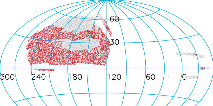
Figure 1.— Aitoff projection of the sky coverage of the cross-correlation samples. The gray region shows the entire SDSS DR7 uniform quasar sample footprint, while the red region shows the current overlap with the DR10 BOSS CMASS galaxy sample.

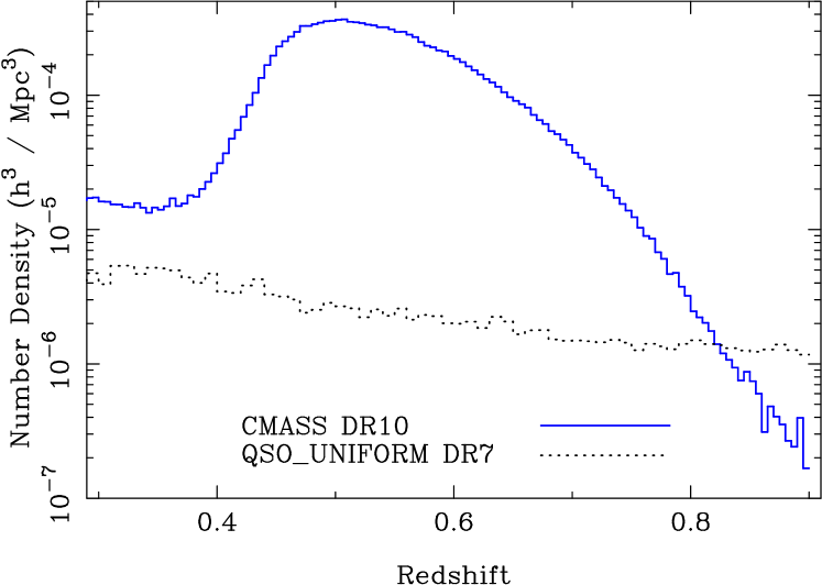
Figure 2.— Number density as a function of redshift for the DR7 uniform quasar and DR10 CMASS galaxy samples. We have limited both samples within $0.3<z<0.9$.

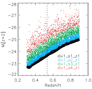
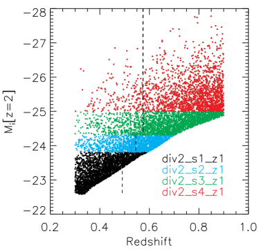
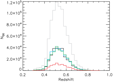
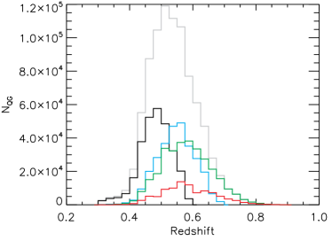
Figure 3.— Subsamples of quasars divided by quasar luminosity. The detailed sample definition is described in §II.2 and summarized in Table 1. The top panels show the distribution in the quasar luminosity-redshift plane, with different colors for the four different luminosity subsamples. Note that the red points overlap with the green points, i.e., the most luminous subsample is a subset of a less luminous subsample. The vertical dashed lines further split each luminosity subsample by the cross-pair-weighted median redshift. The bottom panels show the cross pair-weighted (with $QG$ pair separations $r_{p}<50\,h^{-1}$Mpc and $\pi<70\,h^{-1}$Mpc) redshift distribution of quasars in each subsample (with the gray lines showing that for the full sample). The left and right columns are for Division 1 and Division 2 in terms of quasar luminosity, respectively.

Table 1Summary of Quasar Subsamples. $N^{*}_{\rm QG}$ is the total number of quasar-galaxy pairs with $r_{p}<50\,h^{-1}{\rm Mpc}$ and $\pi<70\,h^{-1}{\rm Mpc}$ in a given cross-correlation sample. The median redshift and magnitude are the pair-count (with $r_{p}<50\,h^{-1}{\rm Mpc}$ and $\pi<70\,h^{-1}{\rm Mpc}$) weighted median values of quasars. The last four columns list the best-fit power-law model correlation length of the CCF (with fixed slope $\gamma=1.7$), the galaxy linear bias, the linear bias of the cross-correlation sample fitted with the full covariance matrix and with diagonal elements of the covariance matrix. See §III for details on subsamples and the estimation of correlation lengths and linear biases.

#	Sample	$N_{\rm Q}$	$N_{\rm G}$	$N_{\rm QG}^{*}$	$z_{\rm min}$	$z_{\rm max}$	$M_{i,\rm{min}}$	$M_{i,\rm{max}}$	$\langle z\rangle$	$\langle M_{i}\rangle$	$r_{0}(\gamma=1.7)$	$b_{\rm G}$	$b_{\rm QG}$	$b_{\rm QG}^{\rm diag}$
0	Full	8198	349608	879352	0.3000	0.8999	$-28.693$	$-22.576$	0.532	$-24.055$	$6.614_{-0.240}^{+0.234}$	$2.10\pm 0.02$	$1.70_{-0.06}^{+0.06}$	$1.70\pm 0.04$
1	div1_s1_z1	2726	349608	293098	0.3003	0.8998	$-25.115$	$-22.576$	0.533	$-23.675$	$6.682_{-0.433}^{+0.414}$	$2.11\pm 0.02$	$1.69_{-0.11}^{+0.11}$	$1.72\pm 0.07$
2	div1_s1_z2	1075	155888	134524	0.3003	0.5320	$-23.819$	$-22.576$	0.481	$-23.440$	$6.390_{-0.654}^{+0.610}$	$2.03\pm 0.04$	$1.44_{-0.17}^{+0.16}$	$1.42\pm 0.10$
3	div1_s1_z3	1651	193720	135256	0.5321	0.8998	$-25.115$	$-23.570$	0.589	$-23.942$	$6.966_{-0.535}^{+0.508}$	$2.15\pm 0.03$	$1.90_{-0.16}^{+0.15}$	$2.01\pm 0.09$
4	div1_s2_z1	2738	349608	293640	0.3002	0.8999	$-25.541$	$-22.808$	0.531	$-24.000$	$6.841_{-0.327}^{+0.316}$	$2.10\pm 0.02$	$1.69_{-0.08}^{+0.08}$	$1.69\pm 0.06$
5	div1_s2_z2	1068	155888	137808	0.3002	0.5319	$-24.171$	$-22.808$	0.480	$-23.726$	$6.899_{-0.463}^{+0.442}$	$2.03\pm 0.04$	$1.69_{-0.11}^{+0.10}$	$1.68\pm 0.08$
6	div1_s2_z3	1670	193720	133358	0.5322	0.8999	$-25.541$	$-23.838$	0.591	$-24.294$	$6.856_{-0.450}^{+0.431}$	$2.15\pm 0.03$	$1.73_{-0.12}^{+0.11}$	$1.72\pm 0.09$
7	div1_s3_z1	2734	349608	292614	0.3000	0.8993	$-28.693$	$-23.208$	0.533	$-24.727$	$6.277_{-0.358}^{+0.344}$	$2.11\pm 0.02$	$1.70_{-0.10}^{+0.09}$	$1.67\pm 0.07$
8	div1_s3_z2	1069	155888	135812	0.3000	0.5319	$-26.851$	$-23.208$	0.481	$-24.395$	$6.823_{-0.607}^{+0.571}$	$2.03\pm 0.04$	$1.78_{-0.15}^{+0.14}$	$1.79\pm 0.09$
9	div1_s3_z3	1665	193720	133933	0.5327	0.8993	$-28.693$	$-24.204$	0.591	$-24.991$	$5.303_{-0.573}^{+0.533}$	$2.15\pm 0.03$	$1.58_{-0.14}^{+0.13}$	$1.52\pm 0.10$
10	div1_s4_z1	837	349608	91081	0.3004	0.8993	$-28.693$	$-23.915$	0.533	$-25.406$	$6.804_{-0.429}^{+0.411}$	$2.11\pm 0.02$	$1.79_{-0.13}^{+0.12}$	$1.78\pm 0.10$
11	div1_s4_z2	321	155888	41766	0.3004	0.5303	$-26.851$	$-23.915$	0.482	$-25.043$	$5.404_{-1.075}^{+0.942}$	$2.03\pm 0.04$	$1.93_{-0.20}^{+0.18}$	$1.88\pm 0.15$
12	div1_s4_z3	516	193720	42015	0.5329	0.8993	$-28.693$	$-24.876$	0.592	$-25.622$	$5.634_{-0.942}^{+0.842}$	$2.15\pm 0.03$	$1.39_{-0.28}^{+0.23}$	$1.42\pm 0.17$
13	div2_s1_z1	2397	249546	283766	0.3000	0.5889	$-23.812$	$-22.576$	0.484	$-23.564$	$6.861_{-0.460}^{+0.439}$	$2.05\pm 0.03$	$1.67_{-0.11}^{+0.10}$	$1.63\pm 0.07$
14	div2_s1_z2	1995	78593	136423	0.3000	0.4906	$-23.810$	$-22.576$	0.448	$-23.420$	$6.797_{-0.655}^{+0.614}$	$2.14\pm 0.05$	$1.55_{-0.16}^{+0.14}$	$1.52\pm 0.10$
15	div2_s1_z3	402	170953	112867	0.4907	0.5889	$-23.812$	$-23.369$	0.524	$-23.659$	$6.429_{-0.689}^{+0.641}$	$2.06\pm 0.04$	$1.69_{-0.19}^{+0.17}$	$1.78\pm 0.10$
16	div2_s2_z1	1443	335123	286117	0.3005	0.6980	$-24.315$	$-23.812$	0.547	$-24.040$	$6.988_{-0.379}^{+0.365}$	$2.11\pm 0.02$	$1.69_{-0.11}^{+0.10}$	$1.69\pm 0.07$
17	div2_s2_z2	628	178865	123829	0.3005	0.5446	$-24.315$	$-23.812$	0.499	$-24.018$	$5.744_{-0.576}^{+0.538}$	$2.05\pm 0.03$	$1.42_{-0.13}^{+0.12}$	$1.44\pm 0.10$
18	div2_s2_z3	815	156258	132738	0.5447	0.6980	$-24.315$	$-23.813$	0.592	$-24.066$	$7.150_{-0.499}^{+0.475}$	$2.12\pm 0.03$	$1.77_{-0.18}^{+0.16}$	$1.84\pm 0.10$
19	div2_s3_z1	4358	349608	306945	0.3004	0.8999	$-28.693$	$-24.315$	0.578	$-24.741$	$5.923_{-0.312}^{+0.301}$	$2.15\pm 0.02$	$1.75_{-0.09}^{+0.09}$	$1.74\pm 0.06$
20	div2_s3_z2	624	229499	138601	0.3004	0.5747	$-26.851$	$-24.315$	0.518	$-24.740$	$6.108_{-0.487}^{+0.461}$	$2.09\pm 0.03$	$1.88_{-0.13}^{+0.13}$	$1.88\pm 0.09$
21	div2_s3_z3	3734	120109	143922	0.5748	0.8999	$-28.693$	$-24.316$	0.637	$-24.744$	$6.259_{-0.371}^{+0.356}$	$2.19\pm 0.04$	$1.77_{-0.09}^{+0.09}$	$1.69\pm 0.07$
22	div2_s4_z1	1966	349608	95949	0.3019	0.8999	$-28.693$	$-25.000$	0.579	$-25.417$	$6.030_{-0.546}^{+0.513}$	$2.15\pm 0.02$	$1.75_{-0.13}^{+0.12}$	$1.70\pm 0.11$
23	div2_s4_z2	188	228104	42244	0.3019	0.5738	$-26.851$	$-25.003$	0.521	$-25.406$	$5.936_{-0.876}^{+0.794}$	$2.09\pm 0.03$	$1.74_{-0.23}^{+0.20}$	$1.69\pm 0.17$
24	div2_s4_z3	1778	121504	45791	0.5745	0.8999	$-28.693$	$-25.000$	0.644	$-25.419$	$6.477_{-0.719}^{+0.667}$	$2.20\pm 0.04$	$1.90_{-0.17}^{+0.16}$	$1.84\pm 0.13$

The SDSS I/II uses a dedicated 2.5-m wide-field telescope (Gunn et al., 2006) with a drift-scan camera with 30 $2048\times 2048$ CCDs (Gunn et al., 1998) to image the sky in five broad bands ($u\,g\,r\,i\,z$; Fukugita et al., 1996). The imaging data are taken on dark photometric nights of good seeing (Hogg et al., 2001), are calibrated photometrically (Smith et al., 2002; Ivezić et al., 2004; Tucker et al., 2006) and astrometrically (Pier et al., 2003), and object parameters are measured (Lupton et al., 2001). Quasar candidates (Richards et al., 2002a) for follow-up spectroscopy are selected from the imaging data using their colors, and are arranged in spectroscopic plates (Blanton et al., 2003) to be observed with a pair of fiber-fed double spectrographs (Smee et al., 2012). The final (DR7) quasar catalog from SDSS I/II was presented in Schneider et al. (2010).

The BOSS survey is an ongoing program within SDSS III (Eisenstein et al., 2011), which is obtaining spectra for massive galaxy and quasar targets selected using photometry from SDSS I/II and new imaging data in the South Galactic Cap (SGC) in SDSS III. Targets are observed with an upgraded version of the multi-object fiber spectrographs for SDSS I/II (Smee et al., 2012). The BOSS spectra are reduced and classified by an automatic pipeline described in Bolton et al. (2012), and the first public data release of BOSS spectra is Data Release 9 (DR9) (Ahn et al., 2012). In this work we use the unpublished Data Release 10 (DR10) for our galaxy sample, which contains BOSS spectra taken through July 2012, and surpasses the DR9 samples.

II.1. Sample Construction

We use the subset of quasars in the SDSS DR7 quasar catalog (Schneider et al., 2010), with UNIFORM_TARGET$=1$ in the value-added catalog of Shen et al. (2011). These quasars were uniformly targeted using the final quasar target selection algorithm (Richards et al., 2002a) implemented in SDSS I/II, and constitute a statistical sample suitable for clustering studies (e.g., Shen et al., 2007, 2009; Ross et al., 2009). For the redshift range of interest here ($z<1$), this quasar sample is flux limited to $i=19.1$. The sky coverage of this uniform quasar sample is 6248 deg².

Two main galaxy samples are targeted in BOSS, with separate color and magnitude cuts: the CMASS sample at $\langle z\rangle\sim 0.55$, and the LOWZ sample at $z\lesssim 0.4$. We choose the CMASS sample as our galaxy sample, as it has a larger redshift overlap with our quasar sample. The total DR10 BOSS CMASS galaxy sample contains over $560\,k$ galaxies, which is approximately one half of the final BOSS CMASS galaxy sample.

Since the CMASS galaxy sample has a narrow redshift distribution that peaks around $z\sim 0.55$ and drops rapidly towards both ends, we have imposed a redshift cut, $0.3<z<0.9$, to both the CMASS sample and the quasar sample. Fig. 1 shows the overlap between the CMASS galaxy sample and the DR7 uniform quasar sample used in the current study, with a sky area of $4122\,{\rm deg}^{2}$. Fig. 2 shows the redshift distributions of our final CMASS sample and quasar sample for subsequent cross-correlation analysis, with 349,608 galaxies and 8,198 quasars in total.

II.2. Quasar Luminosity Subsamples

Since our primary goal is to investigate the luminosity dependence of quasar clustering, we divide our quasar sample into different subsamples by quasar luminosity.

The redshift distributions of the quasars and CMASS galaxies (e.g., Fig. 2) suggest that most of the pair contribution comes from a rather narrow redshift range around $z\sim 0.5$. Thus any redshift-dependent clustering is expected to be small. Nevertheless, we consider quasar subsamples divided by redshift-varying luminosity boundaries (Division 1), as well as by constant luminosity cuts (Division 2), as shown in Fig. 3. Division 1 enforces all subsamples to have the same redshift distribution, but the subsamples will overlap with each other in luminosity. Division 2 ensures there is no luminosity overlap in each subsample, but the effective redshift is slightly different for each subsample. We further split these luminosity subsamples by the pair-weighted quasar median redshift in each bin to create $L-z$ subsamples, to investigate possible redshift evolution. Table 1 summarizes the luminosity and redshift boundaries and properties of these quasar subsamples. These redshift and luminosity boundaries were chosen to yield comparable pair counts for cross-correlation subsamples, except for the most luminous subsamples (div1_s4_* and div2_s4_*).

We assign the effective luminosity and redshift to each quasar subsample using the pair-weighted median values of quasar luminosity and redshift.

II.3. Correcting for Fiber Collisions

Due to restrictions of fiber placement during the BOSS survey, two targets separated by less than 62″ (corresponding to $\sim 0.44\,h^{-1}{\rm Mpc}$ transverse comoving distance at $z=0.55$) cannot be observed simultaneously on the same plate (tile), but can be both observed on overlapping plates. The BOSS tiling procedure uses optimized algorithms to maximize the number of galaxy targets in tile overlap regions, but there are still $\sim 10\%$ CMASS galaxy targets that do not have a spectroscopic observation and are lost from the spectroscopic catalog. This fiber collision effect reduces the number of pairs on small (one-halo) scales and therefore lowers the clustering strength over these small scales. There are several schemes to compensate for the preferential loss of quasar-galaxy pairs due to fiber collisions: upweighting the nearest spectroscopic galaxies that have a collided target (Anderson et al., 2012); assigning the photometric targets a redshift from the nearest spectroscopic neighbor (e.g., Zehavi et al., 2005); or using an algorithm that tracks the tiling geometry and recovers the true small-scale correlation strength (Guo et al., 2012a).

Here we decided to use the upweighting scheme to recover the small-scale cross-correlation signal. In the case of our cross-correlation study, the spectroscopic observations of BOSS galaxies are completely independent of the spectroscopic observations of the low-$z$ SDSS-I/II quasars, as the BOSS survey never places a fiber on a known low-redshift quasar (Ross et al., 2012). The upweighting scheme is thus equivalent to the nearest neighbor scheme such that both methods provide the maximum compensation for pair loss due to fiber collision. The information on the galaxy weights for fiber-collision (and a smaller fraction due to redshift failures) corrections is taken from the DR10 CMASS sample.

II.4. Random Catalogs, Correlation Function Estimators, and Error Estimation

We generate random catalogs for the CMASS galaxy sample with the same angular geometry and redshift distribution as the data. The spectroscopic completeness $f_{s}$ (i.e., fraction of targets with fibers assigned) is a function of sectors (see e.g., Blanton et al., 2003, for the definition of sectors), and is taken into account by upweighting the galaxy points during pair counting. We already account for fiber collisions, so the spectroscopic completeness here does not include objects lost to fiber collisions.

We estimate the 1D and 2D redshift space correlation functions $\xi_{s}(s)$ and $\xi_{s}(r_{p},\pi)$ using the simple estimator (Davis & Peebles, 1983, DP): $QG/QR-1$, where $QG$ and $QR$ are the normalized numbers of quasar-galaxy and quasar-random pairs in each scale bin, $s$ is the pair separation in redshift space, and $r_{p}$ ($\pi$) is the transverse (radial) separation in redshift space. We shall comment further on this choice below. To reduce the effects of redshift distortions, we use the projected correlation function (e.g., Davis & Peebles, 1983)

$$w_{p}(r_{p})=2\int_{0}^{\infty}d\pi\ \xi_{s}(r_{p},\pi)\ .$$ (1)

In practice we integrate $\xi_{s}(r_{p},\pi)$ to $\pi_{\rm max}=70\,h^{-1}$Mpc, where the result is already converged for the scales considered in this paper. This upper-limit of $\pi_{\rm max}$ will be taken into account in our subsequent modeling. For our fiducial $\xi_{s}(r_{p},\pi)$ grid we use a logarithmic binning in $r_{p}$ with $\Delta\log r_{p}=0.125$ starting from $r_{p,{\rm min}}=0.1\,h^{-1}$Mpc and a linear binning in $\pi$ with $\Delta\pi=5\,h^{-1}$Mpc.

There are different methods to estimate the statistical errors of the correlation function measurement, either internally using bootstrap or jackknife resampling, or externally using mock catalogs (for a discussion, see, e.g., Norberg et al., 2009). Here we adopt the jackknife resampling method (as was done in, e.g., Scranton et al., 2002; Zehavi et al., 2005; Shen et al., 2007): we divide the clustering samples into $N_{\rm jack}$ spatially contiguous regions with equal area, and create $N_{\rm jack}$ jackknife samples by excluding each of these regions in turn. We create our jackknife samples using the pixelization scheme of STOMP, which has been used in other studies (e.g., McBride et al., 2011). We measure the correlation function for each of these jackknife samples, and the covariance error matrix is estimated as:

$${\rm Cov}(i,j)=\frac{N_{\rm jack}-1}{N_{\rm jack}}\sum_{l=1}^{N_{\rm jack}}(\xi_{i}^{l}-\bar{\xi}_{i})(\xi_{j}^{l}-\bar{\xi}_{j})\ ,$$ (2)

where indices $i$ and $j$ run over all bins in the correlation function, and $\bar{\xi}$ is the mean value of the statistic $\xi$ over the jackknife samples. The covariance matrix is generally dominated by the diagonal elements except for the large-scale bins, where correlations between adjacent $\xi$ bins become important due to common objects in these bins.

We settled on 50 jackknife samples to estimate the covariance matrix. The normalized covariance matrix (also known as the correlation matrix) is defined as:

$${\rm Cov_{norm}}(i,j)=\frac{{\rm Cov}(i,j)}{\sigma_{i}\sigma_{j}}\ ,$$ (3)

where $\sigma_{i}^{2}\equiv{\rm Cov}(i,i)$ is the diagonal element of the covariance matrix. By default we will use the full covariance matrix in our model fitting unless otherwise stated. Further discussions on error estimations and jackknife sampling are presented in the appendix.

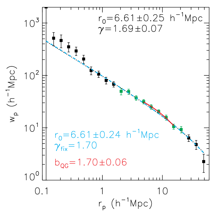
Figure 4.— Projected cross-correlation function for the full quasar and CMASS galaxy cross-correlation sample. The black and cyan lines are the best-fit power-law model for the scale range $r_{p}=2-25\,h^{-1}$Mpc with flexible power-law index $\gamma$ and fixed index $\gamma_{\rm fix}=1.7$. The red line is the best fit linear bias model (i.e., the linear matter correlation function scaled by a constant bias) for the fitting range $r_{p}=4-16\,h^{-1}$Mpc. All fits were performed using the full covariance matrix.

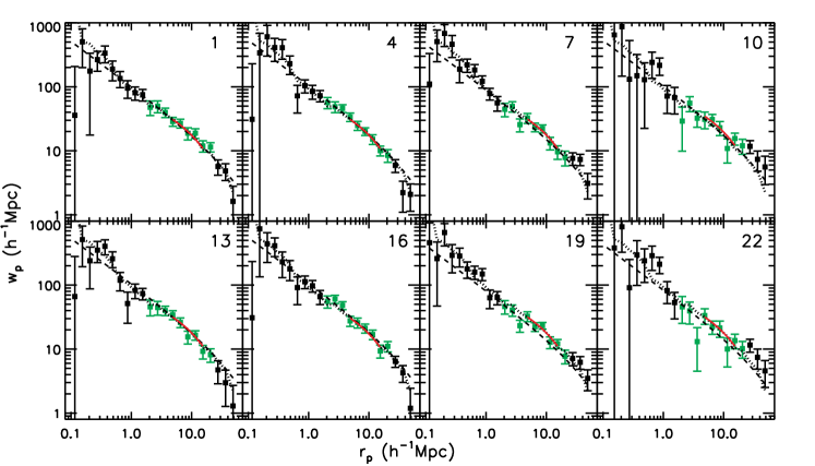
Figure 5.— Projected cross-correlation function for the quasar luminosity subsamples with the two luminosity divisions (see Fig. 3). The data points are measurements for that bin, with green symbols (within $2<r_{p}<25\,h^{-1}{\rm Mpc}$) indicating those used in the power-law model fitting. The $w_{p}$ data for the full sample is shown in dotted lines as a reference. The black dashed lines are the power-law fit to the fitting range $r_{p}=2-25\,h^{-1}$Mpc with fixed slope $\gamma=1.7$, and the red lines are the linear matter correlation function scaled by the best-fit linear bias $b_{QG}$ over the fitting range $r_{p}=4-16\,h^{-1}$Mpc. The sample number is marked in each panel (see Table 1 for sample information).

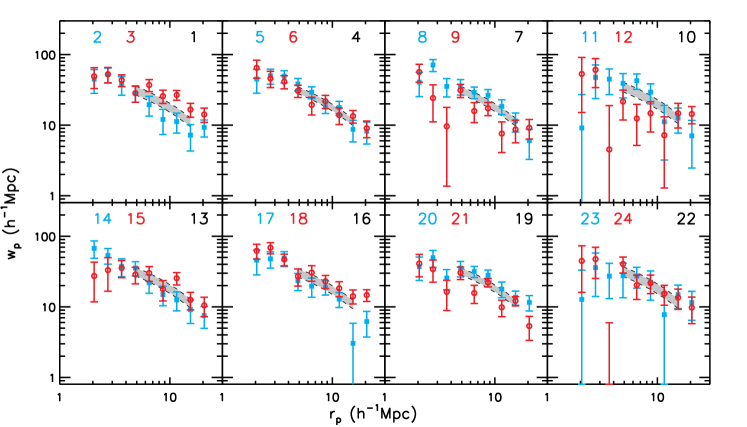
Figure 6.— Projected cross-correlation function for the $L-z$ subsamples with the two luminosity divisions. In each panel, the black shaded region is the 1$\sigma$ range of the biased linear matter correlation function derived from the best-fit to the luminosity subsample indicated by the black number. The cyan and red points are the results for the two $L-z$ subsamples of each luminosity subsample. For clarity we only show the data points over the $2<r_{p}<25\,h^{-1}{\rm Mpc}$ range.

Table 2Measurements of the cross-correlation function $w_{p}$ for the full sample and subsamples. The second column lists the total raw number of $QG$ pairs in a given $r_{p}$ bin with $\pi\leq 70\,h^{-1}{\rm Mpc}$, which can be used as a rough estimate of the robustness of the sample statistics. The last column lists the diagonal errors of the $w_{p}$ measurements, and the normalized covariance matrices are provided in Table 5. A portion is shown here for its content. The table is available in its entirety in the electronic version of this paper.

sample	$r_{p}$	$QG$	$w_{p}$	$\sigma_{w_{p},{\rm diag}}$
#	($h^{-1}$Mpc)		($h^{-1}$Mpc)	($h^{-1}$Mpc)
0	$0.1155$	12	$2061.9628$	$2440.1567$
	$0.1540$	23	$513.5358$	$145.3023$
	$0.2054$	38	$464.1206$	$127.6868$

Table 3Quasar linear bias derived from $b_{QG}$ and $b_{G}$. The error bars are simply propagated from $b_{QG}$ and $b_{G}$ neglecting covariance. We only tabulated the results for the luminosity subsamples (e.g., the results for the $L-z$ subsamples are too noisy to be useful). Note that the data for the most luminous subsample (s4) are a subset of the less luminous subsample (s3), so the bias measurements in these two bins are not independent.

sample	$\langle z\rangle$	$\langle M_{i}\rangle$	$b_{Q}$
Full	0.532	$-24.055$	$1.38\pm 0.10$
div1_s1_z1	0.533	$-23.675$	$1.35\pm 0.18$
div1_s2_z1	0.531	$-24.000$	$1.36\pm 0.13$
div1_s3_z1	0.533	$-24.727$	$1.37\pm 0.15$
div1_s4_z1	0.533	$-25.406$	$1.52\pm 0.21$
div2_s1_z1	0.484	$-23.564$	$1.36\pm 0.17$
div2_s2_z1	0.547	$-24.040$	$1.35\pm 0.17$
div2_s3_z1	0.578	$-24.741$	$1.42\pm 0.15$
div2_s4_z1	0.579	$-25.417$	$1.42\pm 0.20$

III. The Cross Correlation Function

III.1. The whole quasar sample

We show the projected correlation function $w_{p}$ for the full quasar and CMASS galaxy samples in Fig. 4, and tabulate the measurements in Table 2. Much of our focus will be on the larger scales measurements, but it can be seen that we have a good detection of clustering to quite small scales. In particular, there are 842 $QG$ pairs within $r_{p}<1\,h^{-1}{\rm Mpc}$ and $\pi<70\,h^{-1}{\rm Mpc}$, allowing a fair estimate of the small-scale (one-halo) cross-correlation.

We fit the measured CCF with a power-law model $\xi(r)=(r/r_{0})^{-\gamma}$ over the projected scales $2<r_{p}<25\ h^{-1}{\rm Mpc}$ to quantify the clustering strength on intermediate-scales. We can also estimate a linear bias $b_{QG}$, i.e.,

$$w_{p}=w_{p,{\rm matter}}b_{QG}^{2}\ ,$$ (4)

where $w_{p,{\rm matter}}$ is the correlation function of the underlying matter at the redshift of interest, and $b_{QG}^{2}\approx b_{Q}b_{G}$ where $b_{Q}$ and $b_{G}$ are the linear biases for the quasar and CMASS samples respectively.

To estimate the linear bias $b_{QG}$, we use the linear matter correlation function computed using the linear power spectrum in Eisenstein & Hu (1999) under the adopted cosmology, estimated at the pair-weighted median redshift of the cross-correlation samples. Our investigations using mock catalogs (see §IV.3) show that on scales $r_{p}\lesssim 4\,h^{-1}$Mpc nonlinear and one-halo effects start to affect the linear bias, while at $r_{p}\gtrsim 15\,h^{-1}$Mpc residual redshift space distortion (RSD) effects start to become important. Thus we narrow the fitting range to $r_{p}=[4,16]\,h^{-1}$Mpc to estimate the linear bias, where a scale-independent linear bias seems to be a good approximation (within $10\%$). Although we lose statistical power by excluding data points (i.e., only 5 bins of scale are used in the fitting), this procedure is preferred to avoid scales where non-linear effects, scale-dependent bias, and RSDs may affect the linear bias estimate. Nevertheless we tested varying $r_{p}$ boundaries within $[1,50]\,h^{-1}{\rm Mpc}$ in the fitting and found all derived $b_{QG}$ values are consistent within 1$\sigma$, thus our estimate of $b_{QG}$ is robust against this detail.

The correlation function is well fitted by a power-law model with $r_{0}=6.61\pm 0.25$ and $\gamma=1.69\pm 0.07$ over the scales of $2<r_{p}<25\,h^{-1}{\rm Mpc}$ ($\chi^{2}/{\rm dof}=6.54/7$). On smaller scales, the correlation function significantly deviates from the best-fit power-law model derived from larger scales, and requires explicit modeling of the one-halo term. The fact that we detect significant clustering at $r_{p}\lesssim 1\,h^{-1}{\rm Mpc}$ indicates that there are a population of satellite hosted quasars and CMASS galaxies in the cross-correlation sample (see discussions in §IV).

The linear bias for the full cross-correlation sample from our simple fitting is $b_{QG}=1.70\pm 0.06$. In order to derive the quasar linear bias $b_{Q}$ we need to know the linear bias of CMASS galaxies $b_{G}$. For this purpose we have measured the auto correlation function (ACF) for the CMASS galaxy sample using the standard DP estimator, and used the same fitting procedure to estimate $b_{G}$. However, we found that the best-fit $b_{G}$ value does depend on the exact fitting range, given the substantially smaller statistical errors from the ACF measurement. To reduce the risk of contamination from small-scale non-linear clustering and large-scale redshift-space distortion, we fit the CMASS ACF over the same scale range ($r_{p}=[4,16]\,h^{-1}{\rm Mpc}$) as for the CCF data, and derive $b_{G}=2.10\pm 0.02$. Within this fitting range, the ratio of the CCF to the galaxy ACF is roughly constant, allowing use of the relation $b_{QG}^{2}=b_{Q}b_{G}$ to derive the quasar linear bias. The inferred quasar linear bias is $b_{Q}\sim 1.38\pm 0.10$, consistent with the estimated $b_{Q}\sim 1.3\pm 0.2$ from the SDSS quasar auto-correlation function measured at $\langle z\rangle\sim 0.5$ (e.g., Shen et al., 2009). This linear bias is also consistent with the value derived using the HOD approach described in §IV.2 and with the bias of the mock catalogs (which show a slight, slow decrease of the inferred bias from $4\,h^{-1}$Mpc to $16\,h^{-1}$Mpc).

Our derived CMASS galaxy bias value is somewhat larger than the estimated value of $1.8-2$ in other ACF studies of CMASS galaxies (e.g., White et al., 2011; Nuza et al., 2012), but is consistent with that derived in Guo et al. (2012b) based on the DR9 CMASS sample. This result is at least partly caused by the different methodology in estimating the bias. We also compared our ACF measurement directly with those reported in other studies (e.g., White et al., 2011; Anderson et al., 2012; Nuza et al., 2012); our measurement is systematically higher by $\sim 10\%$ over $r_{p}=4-16\,h^{-1}{\rm Mpc}$ scales. To resolve this discrepancy we performed extensive tests upon our galaxy sample and the samples used in other studies, and found that this systematic difference is largely due to the usage of additional galaxy weights in the other studies. While there are good reasons to use those weights in these studies, it is not clear that they are applicable to our cross-correlation measurements. On the other hand, we tested the difference of using the simple DP estimator and the more robust Landy-Szalay (Landy & Szalay, 1993, LS) estimator, and found that the DP estimator over-estimates $w_{p}$ by only $<2\%$ below $r_{p}=10\,h^{-1}{\rm Mpc}$ and by $\sim 10\%$ at $r_{p}\sim 40\,h^{-1}{\rm Mpc}$, which means the difference caused by using the simple DP estimator is negligible. In general the statistical errors tabulated in Table 1 are significantly smaller than the systematic uncertainties in the galaxy bias estimation. Nevertheless, regarding the detection of the luminosity dependence of quasar bias, the exact value of the galaxy bias is not critical.

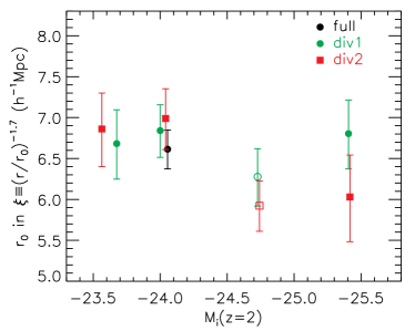
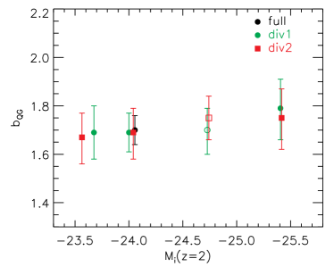
Figure 7.— The strength of the cross-correlation in terms of $r_{0}$ (left) from the power-law model fits and linear bias $b_{QG}$ (right) for different luminosity subsamples. These estimates are tabulated in Table 1. We use open symbols for the second most luminous subsample (s3) in the two divisions to indicate the fact that it contains the most luminous subsample (s4).

      

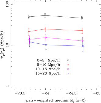
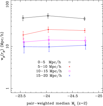
Figure 8.— Clustering in larger (averaged) bins as a function of their median pair-weighted magnitude, for Division 1 (left) and Division 2 (right). Only the first three luminosity subsamples in each division are shown. The errors denote the 1$\sigma$ uncertainty from jackknife re-sampling with 50 regions. This demonstrates that the shape and amplitude of the cross-correlation function show no significant variation for different quasar luminosity subsamples.

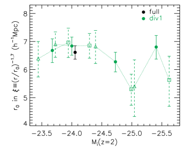
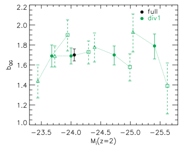
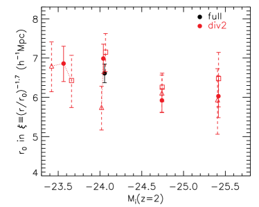
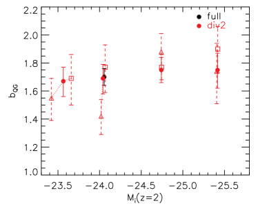
Figure 9.— The strength of the cross-correlation in terms of $r_{0}$ and linear bias $b_{QG}$. For each luminosity subsample we further plot the results of the two redshift subsamples, connected by the dotted lines. No redshift difference is detected given the large error bars.

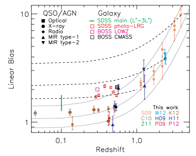
Figure 10.— Left: comparison of the linear bias derived for different tracer samples. The solid symbols are for quasars and AGNs, while the open symbols and the green vertical line segment are for galaxies. Measurements are from Shen et al. (2009, S09), White et al. (2012, W12), Krumpe et al. (2012, K12), Cappelluti et al. (2010, C10), Hickox et al. (2009, H09), Hickox et al. (2011, H11), Zehavi et al. (2011, Z11), Padmanabhan et al. (2009, P09), and Parejko et al. (2012, P12). The three dotted lines are the halo linear bias estimated using the recipes provided in Tinker et al. (2005) for halo masses $M_{h}=1,4,16\times 10^{12}\,h^{-1}M_{\odot}$. Note that different fitting formula for the halo bias will yield slightly different results (e.g., Sheth et al., 2001). The three dashed lines are the predicted bias evolution for a passive population (e.g., Fry, 1996; Mo & White, 1996; Hopkins et al., 2008), started at three arbitrary high redshifts and matched to the measured linear bias of quasars at these redshifts. These biases derived in different work used different methods, and while they often agree within the reported error bars, there are cases when the reported error bars underestimate the systematic uncertainty in determining the bias (e.g., Padmanabhan et al., 2009; Krumpe et al., 2012), especially when the statistical uncertainty is small. With these caveats in mind, this figure suggests that quasars at different redshifts reside in halos with typical masses of a few $10^{12}\,h^{-1}M_{\odot}$, and as such low-redshift quasars are not the descendants of their high-redshift counterparts, which would have evolved into more massive systems. The massive galaxies at $z\lesssim 0.5$ in the SDSS samples typically reside in $\sim 10^{13}\,h^{-1}M_{\odot}$ halos, and could be the descendants of $z\sim 1$ quasars. Right: Same as the left panel, but with the product of the linear bias and the linear growth factor $D(z)$ as the $y$-axis. Thus constant large-scale clustering is denoted by horizontal lines in this plot.

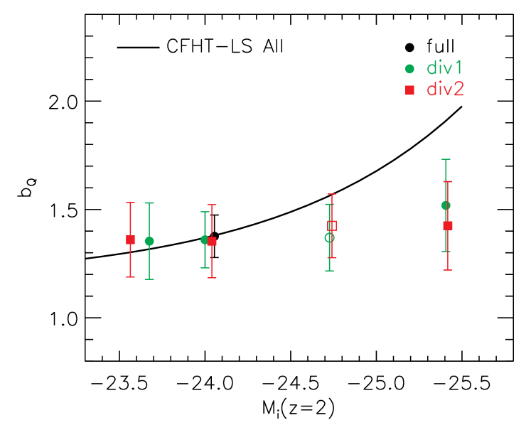
Figure 11.— Comparison of the luminosity dependence of quasar bias derived in this work (symbols) with that of galaxies in the CFHT-LS sample (black solid line) at $0.4<z<0.6$ (Coupon et al., 2012). We use open symbols for the second most luminous subsample (s3) in the two divisions to indicate the fact that it contains the most luminous subsample (s4). To map between quasar luminosity and galaxy luminosity we have assumed that the typical quasar luminosity in our sample ($M_{i}(z=2)=-24.055$) corresponds to the galaxy luminosity with the same bias. Incidently we get a corresponding galaxy luminosity of $\approx L^{*}$. Note that the galaxy biases were derived for luminosity-threshold samples, and we have limited the galaxy luminosity within the range of $0.15-3L^{*}$, approximately the range probed by the CFHT-LS sample. The luminosity dependence of quasar bias is apparently weaker than that of the galaxy bias.

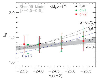
Figure 12.— Left: Comparisons between several model predictions and our measurement of the luminosity dependence of quasar large-scale linear bias. We use open symbols for the second most luminous subsample (s3) in the two divisions to indicate the fact that it contains the most luminous subsample (s4). For the dotted lines (i.e., power-law models with $\alpha=0,0.3,0.6,0.75$), the predictions are generated using the Tinker et al. (2005) halo bias formula at $z=0.53$, and normalized such that they are close to the measured bias for the full quasar sample. The gray band is the prediction at $z=0.5-0.6$ from the Shen (2009) model, and the blue dashed line is the prediction at $z=0.55$ from the fiducial model in Conroy & White (2013, CW13) neglecting the satellite contribution (which serves to increase the bias in the fainter bins by about 5% while leaving the bright bins almost unchanged). Right: The distribution of host halo mass at fixed quasar luminosity from the Shen (2009) model, estimated at $z=0.5$.

III.2. Quasar subsamples divided in luminosity

Fig. 5 shows the resulting cross-correlation function for each quasar luminosity subsample (i.e., no dividing in redshift), and comparison with that for the full sample. For each luminosity subsample we show in Fig. 6 the results for the $L-z$ subsamples. All the measurements are tabulated in Table 2.

Our current samples do not have a sufficient number of small-scale $QG$ pairs ($r_{p}\lesssim 1\,h^{-1}{\rm Mpc}$) to probe the clustering difference on these one-halo scales when dividing our quasar sample in luminosity. To quantify the luminosity-dependence of the large-scale clustering strength we fit $w_{p}$ in the range of $2<r_{p}<25\,h^{-1}{\rm Mpc}$ with the power-law model and in the range of $4<r_{p}<16\,h^{-1}$Mpc with the linear-bias model. For the power-law model we fix the slope to be $\gamma=1.7$, consistent with the best-fit slope for the full cross-correlation sample. The amplitude of the clustering is therefore measured by the best-fit correlation length $r_{0}$ and linear bias $b_{QG}$.

The best-fit values of $r_{0}$ and linear bias $b_{QG}$ for different CCF subsamples are shown in Fig. 7 for the four quasar luminosity subsamples in each division. No significant difference is detected among these subsamples. In Fig. 8 we present the $w_{p}$ values computed over wide linear $r_{p}$ bins with $\Delta r_{p}=5\,h^{-1}{\rm Mpc}$ for the four luminosity subsamples in the two divisions. These $w_{p}$ values represent the averaged correlation over these wide bins. Again, we see that while the value of $w_{p}$ depends on scale, there is no significant difference in clustering strength between any of the samples on these scales. Our sample statistics are insufficient to probe potential luminosity dependence on $r_{p}\lesssim 1\,h^{-1}{\rm Mpc}$ scales.

One concern is that for Div 2 the effective redshift is slightly different for each luminosity subsample, and possible redshift evolution may complicate the interpretation. However, the difference in the linear growth factor over the probed redshift range ($z\sim 0.45-0.65$) is only $\sim 10\%$, and the evolution in the linear bias $b_{G}$ of the CMASS galaxy sample over this redshift range is negligible (see Table 1). Thus the effect of redshift evolution is negligible for our samples, as expected, and we do not observe a significant difference when we further divide our luminosity subsamples in redshift (e.g., Fig. 9).

IV. discussion

The improved measurement of quasar large-scale clustering at $z\sim 0.5$, and the inferred luminosity dependence of quasar bias, can be used to study the evolution of the global quasar population and to test cosmological quasar models while the small-scale cross-correlation probes the immediate neighborhood of quasars and may hint at the triggering mechanism of quasars. Since the statistics on the small-scale cross-correlation in the present study are still not sufficient for detailed studies (see Fig. 5), much of our following discussion will focus on the large-scale quasar bias and its luminosity dependence, although we do attempt to model the small-scale clustering for the full cross-correlation sample.

Quasars reside in dark matter halos, and the redshift evolution of quasar bias can be used to understand the cosmic evolution of this population. A long-lived quasar population may passively evolve into their lower redshift counterparts with a predicted bias evolution (e.g., Fry, 1996; Tegmark & Peebles, 1998; Mo & White, 1996; White et al., 2007; Hopkins et al., 2007a), and can be confronted with the observed quasar bias evolution (see §IV.1).

The observed luminosity dependence of quasar bias constrains how well quasar luminosity correlates with halo mass. In a physical galaxy formation scheme, there are various correlations among halo, galaxy and BH properties such that a chain of $L_{\rm qso}\leftrightarrow M_{\rm BH}\leftrightarrow M_{\rm gal}\leftrightarrow M_{\rm h}$ may form. If the BH mass is more directly connected to halo mass than to galaxy mass, we expect a simpler version, $L_{\rm qso}\leftrightarrow M_{\rm BH}\leftrightarrow M_{\rm h}$. In the simplest scenario, i.e., all quasars are shining at a constant Eddington ratio, and BH mass linearly correlates with halo mass with no scatter, we expect a strong luminosity dependence of quasar bias as a result of more luminous quasars living in more massive halos. In practice, there are inevitably curvature and scatter among these correlations, which will modify the resulting luminosity dependence of quasar bias. For instance, quasar luminosity at fixed BH mass may have a substantial dispersion, as a natural result from different fueling conditions; BH mass may not perfectly (and linearly) correlate with halo mass due to diversities in galaxy formation details. These scatters will produce a distribution of host halo mass at fixed quasar luminosity; the more these halo masses overlap in different quasar luminosity bins, the less prominent will be the observed luminosity dependence of quasar bias. This effect will be further illustrated in the following discussion.

IV.1. Implications from large-scale clustering

Fig. 10 presents the quasar/AGN bias measured in different studies and comparisons to the bias of different galaxy samples. The three dotted lines show the bias of halos with constant halo mass $M_{h}=1,4,16\times 10^{12}\,h^{-1}{\rm Mpc}$ using the Tinker et al. (2005) halo bias formula. The three dashed lines show the evolution of bias for a passive population of tracers (e.g., Fry, 1996; Tegmark & Peebles, 1998; Mo & White, 1996; White et al., 2007; Hopkins et al., 2007a).

These different samples probe different redshifts and luminosities, and are selected with different methods, thus a detailed comparison would be difficult. Furthermore, these studies used different methodologies to estimate the linear bias. Although in most cases the bias values derived with different methods agree to within 1$\sigma$, there are cases where they could differ significantly (e.g., Padmanabhan et al., 2009; Krumpe et al., 2012). Keeping these caveats in mind, some general conclusions can be drawn from this figure:

• Optically selected quasars appear to have a typical halo mass between $10^{12}-10^{13}\,h^{-1}M_{\odot}$ (e.g., Croom et al., 2005; Hopkins et al., 2007a; Shen et al., 2009; Shanks et al., 2011) over a wide redshift range. This result implies that most low-$z$ quasars are not the descendants of their high-$z$ counterparts, which would have evolved into systems with relatively higher bias at low redshift.

• There is no significant difference in the clustering strength between optical quasar samples and several X-ray selected AGN samples at the same redshift (e.g., Krumpe et al., 2012). However, we note that these X-ray AGN samples only probe slightly fainter luminosities than the optical quasar samples, thus both types of active SMBHs are likely drawn from a similar population, and therefore should trace a comparable halo mass range. There may be some hints that radio-selected AGNs have higher clustering than optical quasars and X-ray selected AGNs (e.g., Wake et al., 2008; Hickox et al., 2009; Donoso et al., 2010).

• The galaxy populations from SDSS and BOSS are significantly more clustered than quasars/AGNs at the same redshift. By selection these galaxy samples are at the massive end of the galaxy population. Thus most low-$z$ quasars are not shining within these massive galaxies. These massive galaxies may have experienced a brief quasar phase in the past to build up the central SMBH mass, and are therefore likely the descendants of high-$z$ quasar host galaxies.

At $z\sim 0.5$, the average stellar mass of the CMASS galaxy sample is $\sim 2\times 10^{11}\,M_{\odot}$ (Maraston et al. 2012). This value corresponds to a black hole mass of $\sim 4\times 10^{8}\,M_{\odot}$ using the local $M_{\rm BH}-M_{\rm bulge}$ relation in Marconi & Hunt (2003) and assuming all the stellar mass is in the bulge for CMASS galaxies. The average BH mass of the SDSS quasars is estimated to be $\sim 4\times 10^{7}\,M_{\odot}$ (assuming unity Eddington ratio) or $\sim 3\times 10^{8}\,M_{\odot}$ (virial BH mass estimates from Shen et al. 2011). Since the SDSS quasars reside in halos that are typically a factor of a few less massive than CMASS galaxy hosts, either the quasar BH mass in these lower-mass galaxies is over-massive compared with the prediction from the local $M_{\rm BH}-M_{\rm bulge}$ relation, or the virial mass estimates for SDSS quasars are systematically overestimated (for the latter possibility, see, e.g., Shen et al., 2008; Shen & Kelly, 2010, 2012).

We now examine what constraints the luminosity-dependence of quasar bias at $z\sim 0.5$ can place on cosmological quasar models. First, we derive a quick constraint on the luminosity dependence of quasar bias by fitting a straight line to the data. For simplicity we neglect (small) correlated errors among these bias estimates due to the usage of the common galaxy sample in the cross-correlation measurements. Using the four luminosity subsamples in the two divisions, the slope constrained from the data is

$$\frac{db_{Q}}{d\log L} = 0.20\pm 0.34\quad\textrm{div 1}$$ (5)

$$= 0.11\pm 0.32\quad\textrm{div 2}\ ,$$ (6)

for $-23.5>M_{i}(z=2)>-25.5$. Thus the data are consistent with no luminosity dependence over this luminosity range.

This weak luminosity dependence is in contrast to that of galaxy clustering (e.g., Norberg et al., 2001; Zehavi et al., 2005, 2011; Coil et al., 2008; Coupon et al., 2012). The SDSS main galaxy sample at $\langle z\rangle\sim 0.1$ shows a strong positive luminosity dependence in galaxy clustering (Zehavi et al., 2011): $b_{G}(>L)\times\sigma_{8}/0.8=1.06+0.21(L/L^{*})^{1.12}$, where $L^{*}$ corresponds to $M_{r}=-20.5$. For the $0.4<z<0.6$ galaxies in the Canada-France-Hawaii Telescope Legacy Survey (CFHT-LS) sample (Coupon et al., 2012), $b_{G}(>L)=1.166+0.288(L/L^{*})$ where $L^{*}$ corresponds to $M_{g}^{*}-5\log h=-19.81$ (for all galaxies). The luminosity dependence of galaxy bias for the CFHT-LS sample is shown in Fig. 11 and compared to that of the quasar bias derived in this work. We have assumed that the median quasar luminosity in our sample ($M_{i}(z=2)=-24.055$) corresponds to the galaxy threshold luminosity with the same bias, which incidently corresponds to a galaxy luminosity of $\approx L^{*}$. Based on this comparison, a luminosity dependence of quasar clustering as strong as that for galaxies is ruled out at the $\sim 95\%$ ($\sim 2\sigma$) confidence level (CL). This result reflects a reasonably good correlation between galaxy luminosity (and stellar mass) and halo mass, a correlation that appears to be weaker between quasar luminosity and halo mass.

The linear bias for a population of quasars at fixed luminosity $L$ can be expressed as (e.g., Shen, 2009):

$$b_{Q}(L)=\int b_{h}(M_{h})\frac{dP(M_{h}|L)}{dM_{h}}dM_{h}\ ,$$ (7)

where $b_{h}(M_{h})$ is the linear bias of halos with mass $M_{h}$, and $dP(M_{h}|L)/dM_{h}$ is the distribution of host halo mass at fixed quasar luminosity $L$. If we define an effective halo mass $\langle M_{h}\rangle(L)$ such that $b_{h}(\langle M_{h}\rangle)\equiv b_{Q}(L)$, the dependence of $\langle M_{h}\rangle$ on $L$ determines the luminosity dependence of quasar bias. As a toy model, we parameterize a relation $\langle M_{h}\rangle(L)\propto L^{\alpha}$. A slope of $\alpha\approx 0.6\sim 0.75$ is consistent with a model in which all quasars are shining at fixed Eddington ratio, and their BH mass correlates with halo mass as $M_{\rm BH}\propto M_{h}^{4/3-5/3}$ with no scatter (i.e., a “light bulb” model for quasars). The scaling can be predicted from some analytical arguments (e.g., Silk & Rees, 1998; Wyithe & Loeb, 2003) or inferred from observations of local dormant BHs (e.g., Ferrarese, 2002; Baes et al., 2003) although scatter in the relation is expected. Any scatter in the $M_{\rm BH}-M_{h}$ relation, and dispersion in the Eddington ratio distribution, will lead to flattening in the $\langle M_{h}\rangle-L$ correlation (i.e., reducing $\alpha$). Thus the level of observed luminosity dependence of quasar bias places a constraint on the scatter between halo mass and quasar luminosity for a given power-law slope in the intrinsic correlation.

Fig. 12 (left) shows several realizations of this toy model with different values of $\alpha$ in dotted lines. Models with large $\alpha$ are less favorable compared with the data, although they cannot be completely ruled out given the uncertainties in the measurements.

There are several more realistic, semi-analytical quasar models that can be confronted with this observational constraint (see §I and Appendix B of White et al. 2012). It is beyond the scope of this paper to compare these different models in detail or use our measurements to constrain their model parameters (cf. Shankar et al., 2010a, b).

As a simple demonstration, we consider one semi-analytical quasar model from Shen (2009). This cosmological quasar model assumes that quasars are triggered in halo major mergers, and adopts a quasar light curve model composed of an Eddington-limited accretion phase and a power-law decaying phase. This model can reproduce a variety of quasar observables, including quasar clustering, luminosity function and Eddington ratio distributions over a wide redshift range. In Fig. 12 (left) we show the model predictions for the quasar bias as a function of luminosity at $z=0.5-0.6$ as the gray shaded region. Although this model still predicts a mild increase in quasar bias with luminosity, it matches the data very well. The right panel of Fig. 12 displays the predicted distribution of halo mass for quasars at several fixed luminosities. There is considerable overlap in the range of halo masses for these quasar luminosities, which dilutes the bias difference of these quasars with different luminosities. The large dispersion in halo mass at fixed quasar luminosity is caused by both the scatter between halo mass and BH mass (or peak luminosity) and the luminosity evolution of individual quasars (see discussions in, e.g., Lidz et al., 2006; White et al., 2008; Shen, 2009; Shankar et al., 2010a).

We also compare the data with the prediction from a simple model connecting halos and galaxies to quasars recently proposed by Conroy & White (2013). This model is a “scattered light bulb” model which assumes a linear relation between galaxy mass and quasar BH mass, a lognormal distribution of quasar Eddington ratios, and a constant duty cycle. The free parameters in this model are tuned to match the observed quasar luminosity function over a wide redshift range. The predicted luminosity dependence of quasar bias at $z=0.55$ from their fiducial model (without satellite-hosted quasars) is shown as the blue dashed line in the left panel of Fig. 12. This model predicts a luminosity dependence that is slightly stronger than that predicted by the Shen (2009) model, although it is still consistent with the data within $1\,\sigma$. Inclusion of satellite hosted quasars increases the predicted bias in the fainter bins by about 5% while negligibly changing the brighter bins. This marginally improves the agreement with our data.

One might expect a stronger BH mass dependence of quasar clustering, because the additional scatter between the instantaneous luminosity and BH mass (i.e., the Eddington ratio distribution at fixed BH mass) has no effect here. Quasar BH masses can be estimated with the virial BH mass estimators (e.g., Vestergaard & Peterson, 2006). We tested this hypothesis by dividing the quasar sample using virial BH masses estimated in Shen et al. (2011), but did not find any significant dependence on virial BH mass (also see, e.g., Shen et al., 2009). This result, however, could be due to the large statistical and systematic uncertainties of these virial BH mass estimates (e.g., Shen et al., 2008), or due to a large scatter in the intrinsic correlation between halo mass and quasar BH mass.

IV.2. Halo occupation distribution modeling

Next, we attempt to model our CCF measurements with simple Halo Occupation Distribution (HOD) models (for a review on halo models, see, e.g. Cooray & Sheth, 2002). This approach is an intuitive way to interpret the observed CCF, and can offer insights on how galaxies and quasars form in dark matter halos.

We fix the galaxy HOD by adopting parameters consistent with those in White et al. (2011) from modeling the CMASS galaxy ACF, which reproduces our DR10 CMASS ACF measurement. The large-scale galaxy bias parameter from this set of HOD parameters is $b_{G}=2.00$. For the quasar HOD, we focus on two types of parameterizations. Both types separate the contributions from central and satellite quasars in halos, and they differ in the form of the central quasar HOD. In the first parameterization, the mean number of quasars located at the center of a halo of virial mass $M$ is parameterized as

$$\langle N_{\rm cen}(M)\rangle=\frac{1}{2}\left[1+{\rm erf}\left(\frac{\log M-\log M_{\rm min}}{\sigma_{\rm logM}}\right)\right].$$ (8)

This is a softened step function with characteristic mass scale $M_{\rm min}$ and transition width of $\sigma_{\rm logM}$. We parameterize satellite quasars as a power law with a low mass rolloff,

$$\langle N_{\rm sat}(M)\rangle=\exp\left(-\frac{M_{0}}{M}\right)\left(\frac{M}{M_{1}^{\prime}}\right)^{\alpha}.$$ (9)

Such a quasar HOD parameterization is similar in form to the galaxy HOD (e.g., Zheng et al., 2005, 2007), and it is loosely motivated by cosmological hydrodynamic simulation of AGN (Di Matteo et al., 2008; Chatterjee et al., 2012). This five-parameter model ($M_{\rm min}$, $\sigma_{\rm logM}$, $M_{0}$, $M_{1}^{\prime}$, and $\alpha$) has been applied to model the two-point auto-correlation functions of $\langle z\rangle=1.4$ and $\langle z\rangle=3.2$ SDSS quasars (Richardson et al., 2012). The second quasar HOD parameterization adopts the same satellite HOD form, but it uses a log-normal form for the mean occupation function of central quasars,

$$\langle N_{\rm cen}(M)\rangle=f_{\rm cen}\exp\left[-\frac{(\log M-\log M_{\rm cen})^{2}}{2\sigma_{M}^{2}}\right].$$ (10)

This parameterization has 6 parameters in total (3 for satellite HOD and 3 for central HOD). Compared to the 5-parameter model, it reduces the number of central quasars in massive halos. We will refer to the two types of HOD parameterizations as 5-par and 6-par models, respectively.

For both parameterizations, we assume no correlation between the occupation numbers of central and satellite quasars and between galaxies and quasars. We also assume that the spatial distributions of both quasars and galaxies inside halos follow the Navarro-Frenk-White (NFW) profile (Navarro et al., 1997). The variation and limitation of the quasar HOD parameterizations will be discussed after presenting the main modeling results.

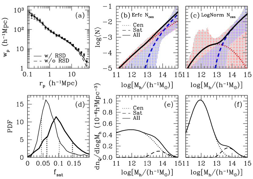
Figure 13.— Results from HOD modeling of the cross-correlation between galaxies and the full sample of quasars. Panel (a): HOD fit to the projected galaxy-quasar CCF. The solid curve is the best-fit from the 5-par HOD model with the effect of residual redshift space distortion (RSD) included. The shaded region is the envelope of the fits from the 68.3% of the models with the smallest $\chi^{2}$ values in the MCMC chain. The dashed curve is the predicted $w_{p}$ with the above best-fit HOD, if the effects of residual RSD were not included. Panel (b): The best-fit mean occupation function of quasars (solid) from the 5-par model, decomposed into its central (dotted) and satellite (dashed) components. The red and blue shaded regions are envelopes from the 68.3% of models with the lowest $\chi^{2}$ values for the central and satellite mean occupation functions. Panel (c): Same as (b), but from the 6-par model. Panel (d): The fraction of satellite quasars in the full sample derived from the HOD modeling. The thin and thick curves are from the 5-par and 6-par models, respectively. Dotted lines enclose the central 68.3% of each distribution. Panel (e): The contribution to the quasar number density as a function of halo mass, decomposed into central (dotted) and satellite (dashed) quasars, from the best-fit 5-par model. The curves are obtained from the product of the mean occupation functions and the differential halo mass function. The curves are also proportional to the probability distribution of host halo mass of quasars. Panel (f): Same as (e), but from the 6-par model. See the text for details on the 5-par and 6-par models.

The calculation of the galaxy-quasar two-point CCF in the HOD framework follows similar procedures in Zheng (2004), Zehavi et al. (2005), and Tinker et al. (2005). One improvement we have in the model is to incorporate the effect of residual redshift-space distortion (RSD) when computing the projected CCF from the real-space CCF, by applying the method of Kaiser (1987) to decompose the CCF into monopole, quadrupole, and hexadecapole moments (also see van den Bosch et al. 2012; J. Tinker, private communication, 2009), which improves the modeling on large scales as we will see later.

We model the cross-correlation between CMASS galaxies and the full sample of quasars at the pair-weighted redshift $z=0.53$. We include the quasar number density in calculating $\chi^{2}$, adopting a value of $2\times 10^{-6}h^{3}{\rm Mpc}^{-3}$ with a 20% fractional error (see Figure 2). A Markov Chain Monte Carlo method is applied to probe the parameter space.

The main results from the HOD modeling are shown in Figure 13. In Figure 13$(a)$, the solid curve is the best-fit $w_{p}$ from the 5-par model, with $\chi^{2}$/dof=26.6/18. The value of $\chi^{2}$ is about 1.4$\sigma$ higher than the expected mean value 18, which is mostly contributed by the three points between $20h^{-1}{\rm Mpc}$ and $40h^{-1}{\rm Mpc}$. While it is an acceptable fit, the slightly higher $\chi^{2}$ may indicate that the model needs further improvement or that the error bars and covariances on large scales are underestimated. The dashed curve shows the predicted $w_{p}$ with the best-fit HOD if the residual RSD is not included in the model. As expected, on scales much less than $\pi_{\rm max}=70h^{-1}{\rm Mpc}$, the effect of residual RSD is small. However, on scales close to $\pi_{\rm max}$, the effect starts to appear, e.g., about 40% lower in $w_{p}$ at $r_{p}\sim 50h^{-1}{\rm Mpc}$ if the residual RSD is neglected. The $\chi^{2}$ from the $w_{p}$ with no RSD becomes $\chi^{2}$/dof=33.3/18, clearly demonstrating that including the residual RSD does improve the fitting significantly.

The best-fit mean occupation functions for the 5-par model are shown in Figure 13$(b)$, which can also be interpreted as the mass-dependent duty cycle of the quasars in the full sample, i.e., the fraction of halos hosting active quasars in the full sample. For central quasars, a large transition width of the softened step function makes $\langle N_{\rm cen}(M)\rangle$ behave like a power law with an index of $\sim 0.8$ above $10^{11}h^{-1}M_{\odot}$. Satellite quasars (with power law index $\sim 1.07$ in $\langle N_{\rm sat}\rangle$ at the high mass end) start to dominate around $10^{14}h^{-1}M_{\odot}$. The overall occupation function resembles a power law with index $\sim 0.95$. The shaded regions delineate the envelopes from the first 68.3% of the models after sorting them in ascending order of $\chi^{2}$, which give us some idea of the constraining power of the CCF on the quasar HOD. For central quasars, the high-mass end is not well constrained – the fast drop in halo mass function toward the massive end makes quasars in massive halos contribute little to the large scale bias and number density of quasars. For satellite quasars, the constraints are tighter around the mass scale where they become comparable in occupation number to the central quasars. This mass scale also corresponds to the mass range of halos that have a significant contribution to small-scale galaxy-quasar pairs. Other than this mass range, the constraints on satellite HOD are loose.

Multiplying the best-fit mean occupation function with the differential halo mass function, we obtain the contribution to the quasar number density from halos of different masses, as shown in Figure 13$(e)$. With appropriate normalization, the curve also gives the probability distribution of the host halo mass of the quasars in the full sample. While peaked around $10^{12}h^{-1}M_{\odot}$, the host halos have a wide distribution in mass, about 4 dex in a full-width-half-maximum sense. Marginalized over all models, the median host halo masses for central and satellite quasars are $\log M_{\rm med,cen}=11.60_{-0.39}^{+0.36}$ and $\log M_{\rm med,sat}=13.74_{-0.39}^{+0.27}$, respectively.

Figure 13$(e)$ demonstrates that satellite quasars (dashed curve) clearly make a non-negligible contribution to the full sample. The strong small-scale clustering in the data requires the existence of satellite quasars. Otherwise, the small-scale $w_{p}$ would become shallower. The satellite fraction marginalized over all models is $f_{\rm sat}=0.068_{-0.023}^{+0.034}$ (the thin curve in Figure 13$(d)$).

With the adopted HOD parameterization, the 5-par model successfully reproduces the observed galaxy-quasar CCF. The central quasar occupation function appears to be a significantly softened step function ($\sigma_{\rm logM}=2.73_{-0.21}^{+0.20}$). Such a large transition width implies a large scatter in quasar luminosity at any given halo mass. The large transition width also leads to a wide mass range of host halos, which even extends to a few times $10^{9}h^{-1}M_{\odot}$, a regime for dwarf galaxies. This result of low mass halos does not appear to be reasonable. Could it be an artifact of the parameterization of the 5-par model? The $\langle N_{\rm cen}(M)\rangle$ function is parameterized to be monotonically increasing with mass towards an asymptotic value of unity (although it never reaches unity in the mass range of interest). There are only two free parameters in $\langle N_{\rm cen}(M)\rangle$, making a relatively tight connection between the high-mass end and the low-mass end HOD. For example, while a higher $\langle N_{\rm cen}(M)\rangle$ at the high mass end helps to reproduce the small-scale clustering, it increases the large-scale bias, and as a response, the occupation function must extend to low-mass halos to reduce the large scale bias.

The 6-par model can explore the parameterization limitation, which allows the high-mass occupation function of central quasars to cutoff exponentially. It tends to mimic the lack of quasar activity in high mass halos where gas accretion is likely suppressed. With this 6-par model, we find an almost equally good fit to $w_{p}$, with $\chi^{2}$/dof=26.1/17, and the best-fit curve is similar to that in Figure 13$(a)$. The constraints on the mean occupation functions (indicated by the shaded regions in Figure 13$(c)$) become less tight, especially for central quasars. The host halo mass for central quasars now has a much narrower distribution (see Figure 13$(f)$), which is in a better agreement with the prediction from the Shen (2009) model (See the right panel in Fig. 12). Marginalized over all models, the median host halo masses for central and satellite quasars are $\log M_{\rm med,cen}=11.85_{-0.33}^{+0.25}$ and $\log M_{\rm med,sat}=13.66_{-0.34}^{+0.26}$, respectively. The satellite fraction from the 6-par model is $f_{\rm sat}=0.099_{-0.036}^{+0.046}$ (see the thick curve in Figure 13$(d)$).

Figure 14.— Top: the mean (total) occupation number of quasars and galaxies for the two quasar HOD parameterization described in §IV.2. The galaxy HOD is the CMASS HOD shifted to lower mass scales to mimic a $L>L^{*}$ galaxy sample, which seems consistent with that in Coupon et al. (2012), and roughly matches the large-scale clustering of quasars. Bottom: the ratio between the mean occupation numbers of quasars and galaxies. The shaded region indicates the $68.3\%$ confidence range. For both quasar HOD parameterizations the ratio of quasars to galaxies rises to a plateau at the high-mass end, but the uncertainties are too large to confirm or rule out a decline in the quasar fraction (per galaxy) in $>10^{14}\,M_{\odot}$ halos (e.g., clusters of galaxies).

The high satellite fraction from either model is a somewhat surprising result. With a similar 5-par parameterization, Richardson et al. (2012) model the 2-point auto-correlation function of $0.5<z<2.5$ ($\bar{z}=1.4$) SDSS quasars and infer a satellite fraction of $(7.4\pm 1.3)\times 10^{-4}$. Also from HOD modeling of quasar clustering, Kayo & Oguri (2012) infer a satellite fraction of $0.054_{-0.016}^{+0.017}$ for $0.6<z<2.2$ quasars. Although our result is close to the latter one, the parameterizations are different — Kayo & Oguri (2012) assumes that both the central and satellite quasar occupation functions have the same Gaussian form, differing only in the amplitudes. The satellite fraction is mainly determined by the small-scale clustering. In detail, for our quasar-galaxy CCF modeling, the result would depend on the assumptions about the correlation between galaxies and quasars inside halos and about the spatial distribution of satellite quasars and galaxies inside halos. This again highlights the ambiguity in HOD parameterizations for the quasar population.

One important distinction is that the quasar satellite fraction in our HOD model is not the fraction of binary quasars (quasar pairs on 1-halo scales). Many of the massive halos will only have one satellite quasar and no central quasar, thus the actual binary quasar fraction would be substantially lower than the satellite fraction. We still designate these quasars as satellite quasars (even though they are the only quasar in the halo) because they have a distinct intra-halo spatial distribution compared to central quasars in our HOD modeling.

The clustering measurement can be well fit using different HOD parameterization, as demonstrated by our 5-par and 6-par models. That is, there exist large degeneracies in quasar HOD from the clustering data alone. In addition to the 2-point correlation functions, we need other observables (e.g., pairwise velocity distribution) to break the degeneracies and constrain the connection between quasars and halos. We also need to rely on theoretical work for a more physically motivated HOD parameterization to model quasar clustering.

We also tried to model the HOD for our quasar luminosity subsamples, but the constraints are poor given the increasingly larger measurement uncertainties. Therefore we defer a more detailed HOD modeling of the luminosity dependence of quasar clustering to future work with improved clustering measurements (especially on small scales, see discussions in § 4.4). The large-scale quasar bias for the full sample from our HOD modeling is: $b=1.27^{+0.08}_{-0.07}$ (5-par) and $b=1.26^{+0.08}_{-0.07}$ (6-par), which are slightly lower, but consistent with our estimation in §III within 1$\sigma$.

Finally, we comment on whether quasars are under-represented in massive halos by examining the ratio of quasars to galaxies as a function of halo mass. Fig. 14 shows the ratio of (central$+$satellite) quasars to galaxies as a function of host halo mass, for the two HOD parameterizations above. For the galaxy HOD we have simply shifted the CMASS HOD to lower mass scales to approximate a $L>L^{*}$ galaxy sample, which seems to be consistent with the results in Coupon et al. (2012), and roughly matches the large-scale clustering of quasars (see Fig. 11 and caption thereof). The quasar-to-galaxy ratio rises to a plateau at high halo masses in both HODs, but the uncertainties are large and we cannot confirm or exclude a decline of quasar fraction (per galaxy) in $\gtrsim 10^{14}\,M_{\odot}$ halos (e.g., clusters of galaxies).

We tabulate the best-fit quasar HOD parameters and the adopted CMASS galaxy HOD parameters in Table 4, but we caution that the quasar HODs are merely for future reference purposes and not for detailed physical interpretation, given the large degeneracies discussed above.

Table 4The adopted CMASS galaxy HOD parameters and the best-fit parameters for the two quasar HOD parameterizations described in §IV.2. All masses are in units of $h^{-1}M_{\odot}$. We caution that the quasar HODs are merely for future reference purposes and not for detailed physical interpretation, given the large degeneracies discussed in §IV.2.

CMASS HOD		5-par quasar HOD		6-par quasar HOD
Eqs. (8) and (9)		Eqs. (8) and (9)		Eqs. (9) and (10)
$\log M_{\rm min}$	$13.14$	$\log M_{\rm min}$	$19.46^{+0.61}_{-0.64}$	$\log M_{\rm cen}$	$13.57^{+4.92}_{-1.41}$
$\sigma_{\log M}$	$0.485$	$\sigma_{\log M}$	$2.73^{+0.20}_{-0.21}$	$\sigma_{M}$	$0.91^{+0.82}_{-0.62}$
$\log M_{0}$	$13.01$	$\log M_{0}$	$12.74^{+0.86}_{-1.05}$	$\log f_{\rm cen}$	$-3.13^{+2.10}_{-0.46}$
$\log M_{1}^{\prime}$	$14.05$	$\log M_{1}^{\prime}$	$16.24^{+0.81}_{-0.51}$	$\log M_{0}$	$12.53^{+0.88}_{-1.02}$
$\alpha$	$0.97$	$\alpha$	$1.19^{+0.37}_{-0.33}$	$\log M_{1}^{\prime}$	$16.13^{+0.73}_{-0.40}$
				$\alpha$	$1.21^{+0.29}_{-0.33}$

IV.3. Mock catalog based interpretation

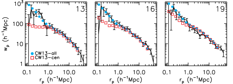
Figure 15.— Comparisons between the measured CCF and predictions from our mock catalogs, for the three luminosity subsamples 13, 16 and 19 (see Table 1). In each panel the black line with error bars is the measured CCF, the red open squares are the prediction for mock quasar model (1) and the cyan filled circles are the prediction for mock quasar model (2). The errors on the predicted CCF are smaller than the observational errors, and are suppressed for clarity. See text for details on the mock catalogs and interpretations.

Figure 16.— Linear and non-linear biases of the CCF from one of our mock catalogs. The underlying matter correlation function was computed using the linear and non-linear power spectra from the simulation directly. The shaded region encloses the $\pm 5\%$ range of the median non-linear bias within $r_{p}=4-16\,h^{-1}$Mpc. Both the linear and non-linear biases show scale-dependence. The non-linear bias is computed using the projected correlation function including redshift space distortions while the linear bias calculation does not include redshift space distortions. For scales $4<r_{p}<16\,{h^{-1}}$Mpc, the linear bias is roughly scale-independent. This result motivated our choice of the fitting range in deriving the linear bias in §III, for which the effects of scale-dependent bias and redshift space distortions are negligible.

We now consider a mock catalog based approach to interpret the observed CCF (e.g. Padmanabhan et al., 2009; White et al., 2011; Conroy & White, 2013). Compared with analytic implementation of the HOD (§IV.2), the mock-based approach directly uses simulated halo catalogs, thus avoiding using any specific fitting formulae for the halo bias and abundance. Unfortunately it can be subject to finite volume and finite resolution limitations. The basis of our catalogs is a $2048^{3}$ particle N-body simulation of the $\Lambda$CDM cosmology in a $700\,h^{-1}$Mpc box run with the TreePM code described in White (2002). This simulation has sufficient volume to probe the CCF on the scales of relevance here while retaining sufficient force and mass resolution to resolve the halos hosting CMASS galaxies and quasars.

We can populate the halos in the simulation using different models for the relevant objects. The CMASS galaxies are placed in the halos using a HOD similar to that described in §IV.2. The parameters are adjusted to fit the small-scale clustering measured in White et al. (2011) and the large-scale clustering measured in Anderson et al. (2012) for CMASS galaxies. Since our purposes are primarily illustrative, we simply chose one model which provides a good fit without attempting to propagate the uncertainty in this model. This best-fit model is a very good fit to the data. For the quasars we chose two different models based on the framework in Conroy & White (2013, CW13 for short). The CW13 framework assumes there is a linear relation between galaxy stellar mass and BH mass with a scatter, and that the BH shines as a quasar with a constant duty cycle, with its luminosity drawn from a lognormal distribution with a constant mean Eddington ratio. This simple model can reproduce the quasar luminosity function and large-scale quasar bias for a wide range of redshifts.

For both quasar models we consider the cross-correlation on both large- and small-scales is independent of the overall duty cycle of the quasars — a random dilution of the sample returns the same clustering on average. The first model assumes quasars live at the centers of dark matter halos with the quasar luminosity set by the stellar mass of the galaxy most likely to be hosted by such a halo (as in Conroy & White, 2013). In the second model, quasars live in both central and satellite galaxies, with the quasar luminosity set by the stellar mass of the galaxy (as in Conroy & White, 2013). Comparison between the two models shows the impact of quasars populating satellite galaxies.

Fig. 15 shows the CCF comparisons of our mock predictions with the data, for the three luminosity subsamples: 13, 16 and 19 in Division 2 (see Table 1). In each panel, the black line with error bars is the measured CCF, and the red (CW13-cen) and cyan (CW13-all) points are our mock predictions for quasar model (1) and (2), respectively. Model (1) where quasars only populate central galaxies does not provide a good match to the small-scale CCF. On the other hand, Model (2) where quasars populate both central and satellite galaxies provides a good match to the overall CCF for three luminosity subsamples (although the model may over-predict the CCF a little on scales of a few $h^{-1}$Mpc for sample 19). The reason that the predicted CCF does not vary much over the three quasar luminosity bins is that there is substantial overlap in the host halo mass range for quasars in the three bins, due to the significant scatter between host galaxy stellar mass and instantaneous quasar luminosity in the CW13 model ($\sim 0.4\,$dex). Since in Model (2), quasars are randomly subsampled from galaxies regardless of their positions (with scatter), the overall satellite fraction of quasars is roughly the same as for galaxies, i.e., $f_{\rm sat}\sim 10\%$ for the three luminosity samples shown in Fig. 15. This satellite fraction is similar to that inferred from the 6-par HOD model discussed in §IV.2. In reality, the situation may be more complicated such that central galaxies might be less likely to host a quasar than satellite galaxies in the most massive halos (e.g., clusters), which will lead to changes in the satellite fraction. In addition, just as for our HOD modeling, any enhanced probability of finding close galaxy-quasar pairs (e.g., if quasars are triggered during interactions with companion galaxies) will change our mock interpretation (which assumes galaxies and quasars are statistically independent when populating the halos). Additional observations of quasars in groups and clusters are required to probe these possibilities.

For our mocks, the mean quasar occupation number and the distribution of host halo mass differ in detail from our best-fit HOD models in §IV.2, which again highlights the fact that there is a broad range of HOD parameter space that can accommodate the observed CCF.

A side product of our mock-based modeling is a prediction for the scale-dependence of the bias for the CCF. In Fig. 16 we show the ratios of the CCF of our mock catalogs to the auto-correlation function of the underlying dark matter computed from the linear and non-linear matter power spectra from our simulation. The linear bias is approximately constant over scales $\sim 4-16\,h^{-1}$Mpc. It is on the basis of this modeling that we have chosen the fitting range quoted in §III.

IV.4. The future

Given the weak luminosity dependence of quasar clustering, one must considerably improve the errors on the measurements to firm up a detection. In addition, it is desirable to have a larger lever arm in quasar luminosity, since the change in quasar linear bias with luminosity is slow. With the cross-correlation technique the galaxy sample limits us to a fixed area of sky. To go brighter we need to work at the highest redshift available (both because of volume effects and because of the $z$-dependence of the luminosity function). To go fainter we need to probe to dimmer objects in the same area of sky.

A major discriminant between quasars models lies in the less luminous quasars (below $L_{\star}$). In older, or more simplified, models these quasars arise from low-mass black holes accreting at close to the Eddington rate, whereas in most modern models a significant fraction of them arise from higher mass black holes accreting at a lower rate (and the prevalence of low accretion rate black holes is particularly pronounced in the redshift range of interest here).

Unlike most galaxy clustering measurements (especially those from SDSS), quasar clustering measurements are still limited by statistical errors. Our current cross-correlation sample only includes $\sim 2/3$ of the final CMASS galaxy-DR7 quasar overlap sample. Thus we expect some improvement in the clustering measurements using the final data release of BOSS. The signal-to-noise ratio for Poisson noise dominated regimes (e.g., at small scales) will increase by a factor of $\sim 1.2$. For large-scale bins where errors are correlated, we expect improvements somewhat smaller than this. In any case, the final cross-correlation sample will have a more uniform sky coverage than the current sample, which may eliminate some systematic problems.

V. conclusions

In this paper we presented the cross-correlation function measurements between quasars and galaxies at $z\sim 0.5$ using a spectroscopic quasar sample from SDSS DR7 and a BOSS CMASS galaxy sample from SDSS-III DR10. Our cross-correlation sample contains 8,198 quasars and 349,608 BOSS (CMASS) galaxies. Our main results are the following:

• The CCF can be well described by a power-law model $\xi_{QG}=(r/r_{0})^{-\gamma}$ for scales $r_{p}=[2,25]\,h^{-1}$Mpc with $r_{0}=6.61\pm 0.25\,h^{-1}$Mpc and $\gamma=1.69\pm 0.07$. The large-scale quasar linear bias is estimated to be $b_{Q}=1.38\pm 0.10$ at $\langle z\rangle\sim 0.53$. This bias infers that quasars at these redshift reside in halos with typical mass of $\sim 4\times 10^{12}\,h^{-1}M_{\odot}$ (using the Tinker et al. 2005 fitting formula), similar to quasar clustering measurements at high-redshift, but lower than the typical halo mass $\sim 10^{13}\,h^{-1}M_{\odot}$ for massive galaxies in SDSS. Thus most of these low-redshift quasars are not the descendants of their high-redshift counterparts, which would have evolved into more massive and more biased systems (such as the hosts of CMASS galaxies).

• We found weak luminosity dependence of the large-scale quasar linear bias, over the luminosity range $-23.5>M_{i}(z=2)>-25.5$ probed by our sample. This result is generally consistent with other quasar clustering measurements at different redshifts. This weak luminosity dependence suggests that quasars with fixed luminosity spread over a broad range of host halo masses, in qualitative and quantitative agreement with predictions from several theoretical models (e.g., Lidz et al., 2006; Shen, 2009; Conroy & White, 2013).

• We performed HOD and mock catalog-based modeling of the measured CCF. For the HOD modeling, we found large degeneracies in the HOD parameterizations such that different HODs can reproduce the CCF equally well, with different host halo mass distributions and satellite fractions. This result highlights the limitations and ambiguities in the standard HOD approach for modeling the quasar population. Additional information is needed in order to break the degeneracies in the quasar HOD models.

  For the mock-based approach, we found the simple model in Conroy & White (2013) that relates quasars to galaxies can reproduce the CCF reasonably well. Under such a model framework, we need a satellite fraction of quasars (i.e., fraction of quasars hosted by satellite galaxies) of $f_{\rm sat}\sim 10\%$. Just as for the HOD-based modeling, however, we cannot rule out other models by which quasars can inhabit dark matter halos and produce the same CCF.

  The difficulty of finding a unique HOD model for quasars probably lies primarily in the fact that quasars are a sparse population with an unknown duty cycle relative to halos (or galaxies). The large scatter between quasar luminosity and halo mass also makes it difficult to use luminosity-dependent clustering as an additional constraint in quasar HOD modeling.

With the upcoming data release of the BOSS survey, we will eventually have a spectroscopic CCF sample with $\sim 50\%$ more quasars and more CMASS galaxies with the final SDSS-III data release. The new data will increase the cross-pair counts by $\sim 50\%$. On small scales ($r_{p}\lesssim 1\,h^{-1}{\rm Mpc}$) where Poisson statistics dominate, we therefore expect $\sim 20\%$ improvement in the errors of $w_{p}$ measurements. These changes will potentially be able to reveal differences in the small-scale clustering when binned in quasar luminosity. In the short term, we also plan to measure the CCF using spectroscopic SDSS-DR7 quasars and the photometric CMASS galaxy sample, which will have the same cross-sample coverage as the final spectroscopic CMASS sample and is free of fiber collision losses. Future deeper galaxy and quasar surveys over large areas can improve the pair statistics further, and at the same time increase the dynamical range in quasar luminosity.

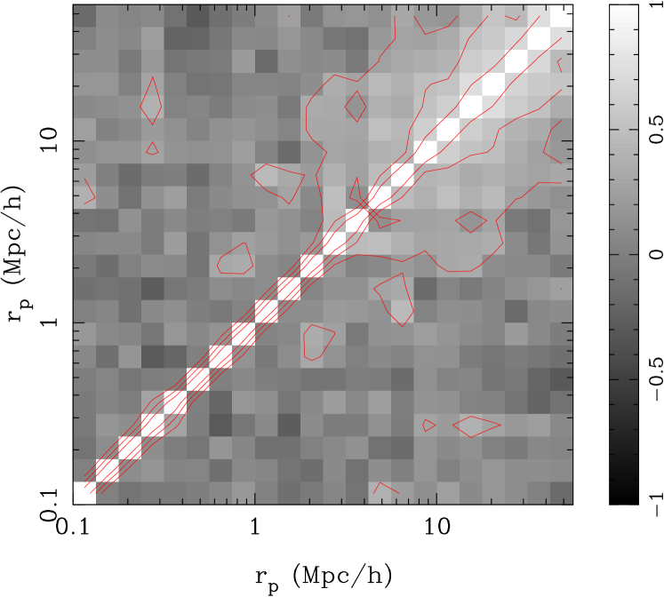
Figure 17.— Correlation matrix of $w_{p}(r_{p})$ for the full sample cross correlation (DR10 CMASS galaxies with DR7 uniform quasars). This is the normalized covariance matrix, i.e. correlation matrix, such that the diagonal elements are unity calculated on 50 jackknife samples. The contours correspond to values of $0.75$, $0.50$, and $0.25$.

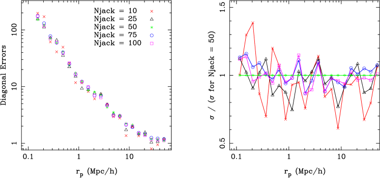
Figure 18.— Left: the 1$\sigma$ (diagonal) errors calculated from varying number of jackknife samples: 10, 25, 50, 75, 100. Our fiducial choice is 50 jackknife samples. Right: the ratio of the diagonal errors with different numbers of jackknife samples to those using 50 jackknife samples.

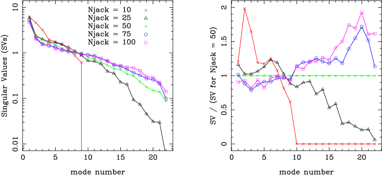
Figure 19.— Singular values (or eigenvalues) obtained by performing a singular value decomposition (SVD) on the correlation matrix estimated from the different number of jackknife samples.

Table 5Normalized covariance matrices from the full CCF sample and from individual CCF subsamples. The corresponding diagonal errors are tabulated in Table 2. A portion (i.e., the covariance matrix from the full CCF sample) is shown here for its content. The table is available in its entirety in the electronic version of this paper.

$r_{p}\ [h^{-1}{\rm Mpc}]$	$0.115$	$0.154$	$0.205$	$0.274$	$0.365$	$0.487$	$0.649$	$0.866$	$1.155$	$1.540$	$2.054$	$2.738$	$3.652$	$4.870$	$6.494$	$8.660$	$11.548$	$15.399$	$20.535$	$27.384$	$36.517$	$48.697$
0.115	$1.000$	$-0.002$	$-0.087$	$-0.047$	$0.001$	$0.137$	$0.015$	$0.141$	$-0.019$	$-0.023$	$-0.161$	$-0.035$	$-0.083$	$0.273$	$0.305$	$0.049$	$0.114$	$-0.086$	$0.078$	$0.123$	$0.022$	$-0.182$
0.154		$1.000$	$0.082$	$0.106$	$0.028$	$-0.010$	$-0.179$	$0.016$	$0.058$	$-0.029$	$-0.116$	$0.104$	$-0.215$	$0.000$	$-0.077$	$0.197$	$0.008$	$0.147$	$0.125$	$0.147$	$0.107$	$0.136$
0.205			$1.000$	$0.055$	$-0.097$	$-0.042$	$0.230$	$0.126$	$-0.164$	$-0.127$	$-0.001$	$0.101$	$0.057$	$-0.155$	$-0.220$	$0.013$	$-0.015$	$0.109$	$-0.070$	$-0.069$	$0.091$	$0.052$
0.274				$1.000$	$0.226$	$0.058$	$-0.375$	$-0.055$	$0.074$	$-0.213$	$0.021$	$-0.078$	$-0.050$	$0.034$	$-0.061$	$0.229$	$0.229$	$0.389$	$0.262$	$0.248$	$0.213$	$0.087$
0.365					$1.000$	$0.071$	$-0.118$	$0.340$	$0.220$	$-0.050$	$0.138$	$0.284$	$0.034$	$0.110$	$-0.006$	$0.068$	$0.089$	$0.144$	$0.002$	$-0.067$	$-0.259$	$0.030$
0.487						$1.000$	$0.027$	$-0.049$	$-0.061$	$0.091$	$-0.068$	$-0.172$	$-0.072$	$-0.077$	$-0.253$	$0.047$	$-0.038$	$0.041$	$-0.190$	$-0.190$	$-0.214$	$-0.302$
0.649							$1.000$	$0.154$	$-0.070$	$0.010$	$0.309$	$0.133$	$0.019$	$-0.007$	$-0.087$	$0.098$	$0.053$	$-0.094$	$-0.068$	$-0.172$	$-0.189$	$-0.210$
0.866								$1.000$	$0.024$	$0.033$	$0.266$	$0.269$	$-0.108$	$0.144$	$0.150$	$0.147$	$0.051$	$0.092$	$0.029$	$0.158$	$-0.088$	$-0.068$
1.155									$1.000$	$-0.087$	$0.140$	$0.180$	$0.070$	$0.170$	$0.389$	$0.123$	$0.124$	$0.194$	$0.082$	$-0.064$	$-0.022$	$0.133$
1.540										$1.000$	$-0.087$	$0.031$	$0.105$	$0.282$	$0.276$	$-0.060$	$0.084$	$0.020$	$0.190$	$0.333$	$0.233$	$0.157$
2.054											$1.000$	$0.231$	$0.047$	$0.091$	$0.097$	$0.076$	$0.280$	$0.245$	$0.127$	$0.072$	$-0.137$	$-0.165$
2.738												$1.000$	$0.389$	$0.350$	$0.166$	$0.297$	$0.153$	$0.336$	$0.285$	$0.077$	$-0.149$	$0.111$
3.652													$1.000$	$0.110$	$0.269$	$0.173$	$0.175$	$0.216$	$0.262$	$0.063$	$-0.011$	$0.208$
4.870														$1.000$	$0.487$	$0.429$	$0.268$	$0.245$	$0.355$	$0.270$	$0.119$	$0.004$
6.494															$1.000$	$0.363$	$0.346$	$0.311$	$0.407$	$0.423$	$0.275$	$0.236$
8.660																$1.000$	$0.496$	$0.598$	$0.547$	$0.294$	$0.224$	$0.207$
11.548																	$1.000$	$0.601$	$0.565$	$0.425$	$0.327$	$0.181$
15.399																		$1.000$	$0.703$	$0.548$	$0.440$	$0.385$
20.535																			$1.000$	$0.679$	$0.488$	$0.482$
27.384																				$1.000$	$0.649$	$0.403$
36.517																					$1.000$	$0.694$
48.697																						$1.000$

The number of jackknife regions is somewhat arbitrary (see detailed discussion in Norberg et al., 2009). Using too few jackknife samples will result in a low number of realizations to estimate the variance, and can formally cause the covariance matrix to become singular (when the number of samples is less than the number of bins). The use of too many jackknife regions causes each region to become small in area (and therefore volume) and can inaccurately represent the cosmic (sample) variance in the large-scale errors. At a minimum, we must ensure the size of each jackknife region is significantly larger than the largest scales we measure in the data.

We first investigate the magnitude of the diagonal errors, which we show in Figure 18. The values of $\sigma$ can vary by up to $30-40$%, but are otherwise roughly equivalent. There is no systematic bias in the values that affects one choice more than any other across all the bins. A lower number of jackknife samples, however, results in a larger variation in the values, as we would expect.

To quantify how well we resolve the structure of the correlation matrix (e.g. Figure 17), we perform a singular value decomposition (SVD) on the correlation matrix. The SVD effectively rotates the matrix into an orthogonal space which can be thought of as a combination of eigenvectors and eigenvalues. The singular values (SVs) are eigenvalues (defined to be positive) which are the multiplicative amplitude of the corresponding (normalized) eigenvector. The SVs are typically numbered such that they are monotonically decreasing, and can be interpreted as a measure of the “importance” of each mode in terms of contributing to the observed structure in the full correlation matrix. For example, an $N$ by $N$ diagonal correlation matrix (i.e. the identity matrix) would result in $N$ SVs that were all equal in value. The ratio of the largest SV divided by the smallest SV is referred to as the condition number, and if significantly large can result in poor numerical results when the matrix is inverted (i.e. an ill-conditioned matrix) which is performed in model fitting.

We show the SVs for our correlation matrices in Figure 19. We clearly see our expectation of the ill-conditioned matrix for $N_{\rm jack}=10$ since we are using 22 bins. A larger $N_{\rm jack}$ results in a better conditioned matrix (a line that appears more flat as the SVs vary less). We also notice quickly diminishing returns for larger numbers of samples: while there is a dramatic difference between $10$ and $50$ samples, it is much less of a difference for the larger numbers of jacknife samples.

We conclude from these investigations that using less than $50$ jackknife samples could be troubling. Taking into account the area coverage of our data ($4122$ deg²), $50$ jackknife samples result in each jackknife region covering about $82$ deg² (roughly $9$ deg or less on a side). As our statistical errors are significantly larger than the galaxy autocorrelation function (e.g. Zehavi et al., 2011), we are not overly concerned about resolving each element of the covariance matrix. Our choice of $50$ jackknife samples is a factor of 2 larger than the number of bins.

References

- Abazajian et al. (2009) Abazajian, K., et al. 2009, ApJS, 182, 543 (DR7)
- Adelberger & Steidel (2005) Adelberger, K. L., & Steidel, C. C. 2005, ApJ, 627, L1
- Ahn et al. (2012) Ahn, C., et al. 2012, ApJS, 203, 21 (DR9)
- Allevato et al. (2011) Allevato, V., et al. 2011, ApJ, 736, 99
- Anderson et al. (2012) Anderson, L., et al. 2012, arXiv:1203.6594
- Baes et al. (2003) Baes, M., Buyle, P., Hau, G. K. T., & Dejonghe, H. 2003, MNRAS, 341, L44
- Bardeen et al. (1986) Bardeen, J. M., Bond, J. R., Kaiser, N., & Szalay, A. S. 1986, ApJ, 304, 15
- Blanton et al. (2003) Blanton, M. R., Lin, H., Lupton, R. H., Maley, F. M., Young, N., Zehavi, I., & Loveday, J. 2003, AJ, 125, 2276
- Bolton et al. (2012) Bolton, A., et al. 2012, AJ, 144, 144
- Bonoli et al. (2009) Bonoli, S., Marulli, F., Springel, V., White, S. D. M., Branchini, E., & Moscardini, L. 2009, MNRAS, 396, 423
- Cao (2010) Cao, X. 2010, ApJ, 725, 388
- Cappelluti et al. (2010) Cappelluti, N. , Ajello, M., Burlon, D., Krumpe, M., Miyaji, T., Bonoli, S., & Greiner, J. 2010, ApJ, 716, L209
- Chatterjee et al. (2012) Chatterjee, S., Degraf, C., Richardson, J., Zheng, Z., Nagai, D., & Di Matteo, T. 2012, MNRAS, 419, 2657
- Cohn & White (2008) Cohn J.D., White M., 2008, MNRAS, 385, 2025.
- Coil et al. (2006) Coil, A. L., Newman, J. A., Cooper, M. C., Davis, M., Faber, S. M., Koo, D. C., & Willmer, C. N. A. 2006, ApJ, 644, 671
- Coil et al. (2007) Coil, A. L., Hennawi, J. F., Newman, J. A., Cooper, M. C., & Davis, M. 2007, ApJ, 654, 115
- Coil et al. (2008) Coil, et al., 2008, ApJ, 672, 153
- Coil et al. (2009) Coil, A. L., et al. 2009, ApJ, 701, 1484
- Cole & Kaiser (1989) Cole, S., & Kaiser, N. 1989, MNRAS, 237, 1127
- Conroy & White (2013) Conroy, C., & White, M. 2013, ApJ, in press, arXiv:1208.3198
- Cooray & Sheth (2002) Cooray, A., & Sheth, R. 2002, Phys. Rep., 372, 1
- Coupon et al. (2012) Coupon, J., et al. 2012, A&A, 542, 5
- Croom et al. (2004) Croom, S. M., Smith, R. J., Boyle, B. J., Shanks, T., Miller, L., Outram, P. J., & Loaring, N. S. 2004, MNRAS, 349, 1397
- Croom et al. (2005) Croom, S. M., et al. 2005, MNRAS, 356, 415
- Croton (2009) Croton, D. J. 2009, MNRAS, 394, 1109
- da Ângela et al. (2005) da Ângela, J., Outram, P. J., Shanks, T., Boyle, B. J., Croom, S. M., Loaring, N. S., Miller, L., & Smith, R. J. 2005, MNRAS, 360, 1040
- da Ângela et al. (2008) da Ângela, J., et al. 2008, MNRAS, 383, 565
- Davis & Peebles (1983) Davis, M., & Peebles, P. J. E. 1983, ApJ, 267, 465
- Dawson et al. (2012) Dawson, K. S., et al. 2012, submitted, arXiv:1208.0022
- Degraf et al. (2011) Degraf, C., Di Matteo, T., & Springel, V. 2011, MNRAS, 413, 1383
- Di Matteo et al. (2008) Di Matteo, T., Colberg, J., Springel, V., Hernquist, L., & Sijacki, D. 2008, ApJ, 676, 33
- Donoso et al. (2010) Donoso, E., Li, C. Kauffmann, G. Best, P. N., & Heckman, T. M. 2010, MNRAS, 407, 1078
- Eisenstein & Hu (1999) Eisenstein, D. J., & Hu, W. 1999, ApJ, 511, 5
- Eisenstein et al. (2011) Eisenstein, D. J., et al. 2011, AJ, 142, 72
- Fanidakis et al. (2012) Fanidakis N., Baugh C.M., Benson A.J., Bower R.G., Cole S., Done C., Frenk C.S., Hickox R.C., Lacey C., del P. Lagos C., 2012, MNRAS, 419, 2797
- Ferrarese (2002) Ferrarese, L. 2002, ApJ, 578, 90
- Fry (1996) Fry, J. N. 1996, ApJ, 461, L65
- Fukugita et al. (1996) Fukugita, M., Ichikawa, T., Gunn, J. E., Doi, M., Shimasaku, K., & Schneider, D. P. 1996, AJ, 111, 1748
- Gilli et al. (2009) Gilli, R., et al. 2009, A&A, 494, 33
- Gunn et al. (1998) Gunn, J. E., et al. 1998, AJ, 116, 3040
- Gunn et al. (2006) —. 2006, AJ, 131, 2332
- Guo et al. (2012a) Guo, H., Zehavi, I., & Zheng, Z. 2012a, ApJ, 756, 127
- Guo et al. (2012b) Guo, H., et al. 2012b, ApJ, submitted, arXiv:1212.1211
- Haiman & Hui (2001) Haiman, Z., & Hui, L. 2001, ApJ, 547, 27
- Hennawi et al. (2006) Hennawi, J. F., et al. 2006, AJ, 131, 1
- Hickox et al. (2009) Hickox, R. C., et al. 2009, ApJ, 696, 891
- Hickox et al. (2011) —. 2011, ApJ, 731, 117
- Hirschmann et al. (2012) Hirschmann M., Somerville R. S., Naab T., Burkert A. 2012, MNRAS, 426, 237
- Hogg et al. (2001) Hogg, D. W., Finkbeiner, D. P., Schlegel, D. J., & Gunn, J. E. 2001, AJ, 122, 2129
- Hopkins et al. (2008) Hopkins, P. F., Hernquist, L., Cox, T. J., & Kereš, D. 2008, ApJS, 175, 356
- Hopkins et al. (2005) Hopkins, P. F., Hernquist, L., Martini, P., Cox, T. J., Robertson, B., Di Matteo, T., & Springel, V. 2005, ApJ, 625, L71
- Hopkins et al. (2007a) Hopkins, P. F., Lidz, A., Hernquist, L., Coil, A. L., Myers, A. D., Cox, T. J., & Spergel, D. N. 2007a, ApJ, 662, 110
- Ivashchenko et al. (2010) Ivashchenko, G., Zhdanov, V. I., & Tugay, A. V. 2010, MNRAS, 409, 1691
- Ivezić et al. (2004) Ivezić, Ž., et al. 2004, Astronomische Nachrichten, 325, 583
- Kaiser (1987) Kaiser, N. 1987, MNRAS, 227, 1
- Kayo & Oguri (2012) Kayo, I. and Oguri, M. 2012, MNRAS, 424, 1363
- Komatsu et al. (2011) Komatsu, E., et al. 2011, ApJS, 192, 18
- Krumpe et al. (2010) Krumpe, M., Miyaji, T., & Coil, A. L. 2010, ApJ, 713, 558
- Krumpe et al. (2012) Krumpe, M., Miyaji, T., Coil, A. L., & Aceves, H. 2012, ApJ, 746, 1
- Landy & Szalay (1993) Landy, S. D., & Szalay, A. S. 1993, ApJ, 412, 64
- Li et al. (2006) Li, C., Kauffmann, G., Wang, L., White, S. D. M., Heckman, T. M., & Jing, Y. P. 2006, MNRAS, 373, 457
- Lidz et al. (2006) Lidz, A., Hopkins, P. F., Cox, T. J., Hernquist, L., & Robertson, B. 2006, ApJ, 641, 41
- Lupton et al. (2001) Lupton, R., Gunn, J. E., Ivezić, Z., Knapp, G. R., & Kent, S. 2001, in Astronomical Society of the Pacific Conference Series, Vol. 238, Astronomical Data Analysis Software and Systems X, ed. F. R. Harnden, Jr., F. A. Primini, & H. E. Payne, 269
- Maraston et al. (2012) Maraston, C., et al. 2012, arXiv:1207.6114
- Marconi & Hunt (2003) Marconi, A., & Hunt, L. K. 2003, ApJ, 589, L21
- Martini & Weinberg (2001) Martini, P., & Weinberg, D. H. 2001, ApJ, 547, 12
- McBride et al. (2011) McBride, C. K. and Connolly, A. J. and Gardner, J. P. and Scranton, R. and Newman, J. A. and Scoccimarro, R. and Zehavi, I. and Schneider, D. P. 2011, ApJ, 726, 13
- Miyaji et al. (2011) Miyaji, T., Krumpe, M., Coil, A. L., & Aceves, H. 2011, ApJ, 726, 83
- Mo & White (1996) Mo, H. J., & White, S. D. M. 1996, MNRAS, 282, 347
- Myers et al. (2007a) Myers, A. D., Brunner, R. J., Nichol, R. C., Richards, G. T., Schneider, D. P., & Bahcall, N. A. 2007a, ApJ, 658, 85
- Myers et al. (2007b) Myers, A. D., Brunner, R. J., Richards, G. T., Nichol, R. C., Schneider, D. P., & Bahcall, N. A. 2007b, ApJ, 658, 99
- Myers et al. (2008) Myers, A. D., Richards, G. T., Brunner, R. J., Schneider, D. P., Strand, N. E., Hall, P. B., Blomquist, J. A., & York, D. G. 2008, ApJ, 678, 635
- Myers et al. (2006) Myers, A. D., et al. 2006, ApJ, 638, 622
- Navarro et al. (1997) Navarro, J. F., Frenk, C. S., & White, S. D. M. 1997, ApJ, 490, 493
- Norberg et al. (2001) Norberg, P., et al., 2001, MNRAS, 328, 64
- Norberg et al. (2009) Norberg, P., Baugh, C. M., Gaztañaga, E., & Croton, D. J. 2009, MNRAS, 396, 19
- Nuza et al. (2012) Nuza, S. E., et al. 2012, MNRAS, in press, arXiv:1202.6057
- Padmanabhan et al. (2009) Padmanabhan, N., White, M., Norberg, P., & Porciani, C. 2009, MNRAS, 397, 1862
- Parejko et al. (2012) Parejko, J., et al. 2012, MNRAS, submitted
- Pier et al. (2003) Pier, J. R., Munn, J. A., Hindsley, R. B., Hennessy, G. S., Kent, S. M., Lupton, R. H., & Ivezić, Ž. 2003, AJ, 125, 1559
- Porciani et al. (2004) Porciani, C., Magliocchetti, M., & Norberg, P. 2004, MNRAS, 355, 1010
- Porciani & Norberg (2006) Porciani, C., & Norberg, P. 2006, MNRAS, 371, 1824
- Richards et al. (2002a) Richards, G. T., et al. 2002a, AJ, 123, 2945
- Richards et al. (2006) Richards, G. T. et al. 2006, AJ, 131, 2766
- Richardson et al. (2012) Richardson, J., Zheng, Z., Chatterjee, S., Nagai, D., & Shen, Y. 2012, ApJ, 755, 30
- Ross et al. (2009) Ross, N. P., et al. 2009, ApJ, 697, 1634
- Ross et al. (2012) Ross, N. P., et al. 2012, ApJS, 199, 3
- Sanchez et al. (2012) Sanchez A.G., et al., 2012, submitted, arXiv:1203.6616
- Schlegel, White & Eisenstein (2009) Schlegel D., White M., Eisenstein D.J., 2009, The Astronomy and Astrophysics Decadal Survey, Science White Papers #314, arXiv:0902.4680
- Scranton et al. (2002) Scranton, R., et al. 2002, ApJ, 579, 48
- Schneider et al. (2010) Schneider, D. P., et al. 2010, AJ, 139, 2360
- Shankar et al. (2009) Shankar, F., Weinberg, D. H., & Miralda-Escudé, J. 2009, ApJ, 690, 20
- Shankar et al. (2010b) Shankar, F., Crocce, M., Miralda-Escudé, J., Fosalba, P., & Weinberg, D. H. 2010, ApJ, 718, 231
- Shankar et al. (2010a) Shankar, F., Weinberg, D. H., & Shen, Y. 2010, MNRAS, 406, 1959
- Shanks et al. (2011) Shanks, T., Croom, S. M., Fine, S., Ross, N. P., & Sawangwit, U. 2011, MNRAS, 416, 650
- Shaver (1984) Shaver, P. A. 1984, A&A, 136, L9
- Shen (2009) Shen, Y. 2009, ApJ, 704, 89
- Shen et al. (2008) Shen, Y., Greene, J. E., Strauss, M. A., Richards, G. T., & Schneider, D. P. 2008, ApJ, 680, 169
- Shen et al. (2008) Shen, Y., Strauss, M. A., Hall, P. B., Schneider, D. P., York, D. G., & Bahcall, N. A. 2008, ApJ, 677, 858
- Shen & Kelly (2010) Shen, Y., & Kelly, B. C. 2010, ApJ, 713, 41
- Shen & Kelly (2012) —. 2012, ApJ, 746, 169
- Shen et al. (2007) Shen, Y., et al. 2007, AJ, 133, 2222
- Shen et al. (2009) —. 2009, ApJ, 697, 1656
- Shen et al. (2010) —. 2010, ApJ, 719, 1693
- Shen et al. (2011) —. 2011, ApJS, 194, 45
- Sheth et al. (2001) Sheth, R. K., Mo, H. J., & Tormen, G. 2001, MNRAS, 323, 1
- Silk & Rees (1998) Silk, J., & Rees, M. J. 1998, A&A, 331, L1
- Smee et al. (2012) Smee, S. A., et al. 2012, AJ, submitted, arXiv:1208.2233
- Smith et al. (2002) Smith, J. A., et al. 2002, AJ, 123, 2121
- Tegmark & Peebles (1998) Tegmark, M., & Peebles, P. J. E. 1998, ApJ, 500, L79
- Thacker et al. (2009) Thacker, R. J., Scannapieco, E., Couchman, H. M. P., & Richardson, M. 2009, ApJ, 693, 552
- Tinker et al. (2005) Tinker, J. L., Weinberg, D. H., Zheng, Z., & Zehavi, I. 2005, ApJ, 631, 41
- Tucker et al. (2006) Tucker, D. L., et al. 2006, Astronomische Nachrichten, 327, 821
- van den Bosch et al. (2012) van den Bosch, F., More, S., Cacciato, M., Mo, H., & Yang, X. 2012, arXiv:1206.6890
- Vestergaard & Peterson (2006) Vestergaard, M., & Peterson, B. M. 2006, ApJ, 641, 689
- Wake et al. (2008) Wake, D. A., Croom, S. M., Sadler, E. M., & Johnston, H. M. 2008, MNRAS, 391, 1674
- White (2002) White M., 2002, ApJS, 579, 16
- White et al. (2008) White, M., Martini, P., & Cohn, J. D. 2008, MNRAS, 390, 1179
- White et al. (2007) White, M., Zheng, Z., Brown, M.J.I., Dey, A., Jannuzi, B.T., 2007, ApJ, 655, L69
- White et al. (2011) White, M., et al. 2011, ApJ, 728, 126
- White et al. (2012) White, M., et al. 2012, MNRAS, 424, 933
- Wyithe & Loeb (2003) Wyithe, J. S. B., & Loeb, A. 2003, ApJ, 595, 614
- York et al. (2000) York, D. G., et al. 2000, AJ, 120, 1579
- Yu & Lu (2004) Yu, Q., & Lu, Y. 2004, ApJ, 602, 603
- Yu & Lu (2008) —. 2008, ApJ, 689, 732
- Zehavi et al. (2005) Zehavi, I., et al. 2005, ApJ, 630, 1
- Zehavi et al. (2011) —. 2011, ApJ, 736, 59
- Zheng (2004) Zheng, Z. 2004, ApJ, 610, 61
- Zheng et al. (2005) Zheng, Z., Berlind, A. A., Weinberg, D. H., et al. 2005, ApJ, 633, 791
- Zheng et al. (2007) Zheng, Z., Coil, A. L., & Zehavi, I. 2007, ApJ, 667, 760