Exponential Error Bounds on Parameter Modulation–Estimation for Discrete Memoryless Channels

Abstract

We consider the problem of modulation and estimation of a random parameter $U$ to be conveyed across a discrete memoryless channel. Upper and lower bounds are derived for the best achievable exponential decay rate of a general moment of the estimation error, $\mbox{\boldmath$E$}|\hat{U}-U|^{\rho}$, $\rho\geq 0$, when both the modulator and the estimator are subjected to optimization. These exponential error bounds turn out to be intimately related to error exponents of channel coding and to channel capacity. While in general, there is some gap between the upper and the lower bound, they asymptotically coincide both for very small and for very large values of the moment power $\rho$. This means that our achievability scheme, which is based on simple quantization of $U$ followed by channel coding, is nearly optimum in both limits. Some additional properties of the bounds are discussed and demonstrated, and finally, an extension to the case of a multidimensional parameter vector is outlined, with the principal conclusion that our upper and lower bound asymptotically coincide also for a high dimensionality.

Index Terms: Parameter estimation, modulation, discrete memoryless channels, error exponents, random coding, data processing theorem.

1 Introduction

Consider the problem of conveying the value of a parameter $u$ across a given discrete memoryless channel

$$p(\mbox{\boldmath$y$}|\mbox{\boldmath$x$})=\prod_{t=1}^{n}p(y_{t}|x_{t}),$$ (1)

where $\mbox{\boldmath$x$}=(x_{1},\ldots,x_{n})$ and $\mbox{\boldmath$y$}=(y_{1},\ldots,y_{n})$ are the channel input and output vectors, respectively. Our main interest, in this work, is in the following questions: How well can one estimate $u$ based on $y$ when one is allowed to optimize, not only the estimator, but also the modulator, that is, the function $\mbox{\boldmath$x$}(u)=(x_{1}(u),\ldots,x_{n}(u))$ that maps $u$ into a channel input vector? How fast does the estimation error decay as a function of $n$ when the best modulator and estimator are used?

In principle, this problem, which is the discrete–time analogue of the classical problem of “waveform communication” (in the terminology of [15, Chap. 8]), can be viewed both from the information–theoretic and the estimation–theoretic perspectives. Classical results in neither of these disciplines, however, seem to suggest satisfactory answers.

From the information–theoretic point of view, if the parameter is random, call it $U$, this is actually a problem of joint source–channel coding, where the source emits a single variable $U$ (or a fixed number of them when $U$ is a vector), whereas the channel is allowed to be used many times ($n$ is large). The separation theorem of classical information theory asserts that asymptotic optimality of separate source– and channel coding is guaranteed in the limit of long blocks. However, it refers to a regime of long blocks both in source coding and channel coding, whereas here the source block length is 1, and so, there is no hope to compress the source with performance that comes close to the rate–distortion function.

In the realm of estimation theory, on the other hand, there is a rich literature on Bayesian and non–Bayesian bounds, mostly concerning the mean square error (MSE) in estimating parameters from signals corrupted by an additive white Gaussian noise (AWGN) channel, as well as other channels (see, e.g., [12] and the introductions of [1], [2], and [14] for overviews on these bounds). Most of these bounds lend themselves to calculation for a given modulator $\mbox{\boldmath$x$}(u)$ and therefore they may give insights concerning optimum estimation for this specific modulator. They may not, however, be easy to use for the derivation of universal lower bounds, namely, lower bounds that depend neither on the modulator nor on the estimator, which are relevant when both optimum modulators and optimum estimators are sought. Two exceptions to this rule (although usually, not presented as such) are families of bounds that stem from generalized data processing theorems (DPT’s) [5], [6], [11], [16], [18], henceforth referred to as “DPT bounds”, and bounds based on hypothesis testing and channel coding considerations [1], [3], [17], henceforth called “channel–coding bounds.”

In this paper, we use both the channel–coding techniques and DPT techniques in order to derive lower bounds on general moments of the estimation error, $\mbox{\boldmath$E$}|\hat{U}-U|^{\rho}$, where $U$ is a random parameter, $\hat{U}$ is its estimate, and the power $\rho$ is an arbitrary positive real (not necessarily an integer). It turns out that when $\mbox{\boldmath$x$}(u)$ is subjected to optimization, $\mbox{\boldmath$E$}|\hat{U}-U|^{\rho}$ can decay exponentially rapidly as a function of $n$, and so, our focus is on the best achievable exponential rate of decay as a function of $\rho$, which we shall denote by ${\cal E}(\rho)$, that is,

$$\inf\mbox{\boldmath$E$}|\hat{U}-U|^{\rho}\approx e^{-n{\cal E}(\rho)},$$ (2)

where the infimum is over all modulators and estimators. Interestingly, both the upper and lower bounds on ${\cal E}(\rho)$ are intimately related to well–known exponential error bounds associated with channel coding, such as Gallager’s random coding exponent (for small values of $\rho$) and the expurgated exponent function (for large values of $\rho$). In other words, we establish an estimation–theoretic meaning to these error exponent functions. In particular, under certain conditions, our channel–coding upper bound on ${\cal E}(\rho)$ (corresponding to a lower bound on $\mbox{\boldmath$E$}|\hat{U}-U|^{\rho}$) can be presented as

$$\overline{E}(\rho)=\left\{\begin{array}[]{ll}E_{0}(\rho)&\rho<\rho_{0}\\ E_{ex}(0)&\rho\geq\rho_{0}\end{array}\right.$$ (3)

where $E_{0}(\rho)=\max_{q}E_{0}(\rho,q)$, $E_{0}(\rho,q)$ being Gallager’s function, $E_{ex}(0)$ is the expurgated exponent at zero rate, and $\rho_{0}$ is value of $\rho$ for which $E_{0}(\rho)=E_{ex}(0)$ (so that $\overline{E}(\rho)$ is continuous). In addition, we derive a DPT bound and discuss its advantages and disadvantages compared to the above bound.

We also suggest a lower bound, $\underline{E}(\rho)$, on ${\cal E}(\rho)$ (associated with upper bounds on $\inf\mbox{\boldmath$E$}|\hat{U}-U|^{\rho}$), which is achieved by a simple, separation–based modulation and estimation scheme. While there is a certain gap between $\overline{E}(\rho)$ and $\underline{E}(\rho)$ for every finite $\rho$, it turns out that this gap disappears (in the sense that the ratio $\underline{E}(\rho)/\overline{E}(\rho)$ tends to unity) both for large $\rho$ and for small $\rho$, and so, we have exact asymptotics of ${\cal E}(\rho)$ in these two extremes: For large $\rho$, ${\cal E}(\rho)$ tends to $E_{ex}(0)$ and for small $\rho$, ${\cal E}(\rho)\sim\rho C$, where $C$ is the channel capacity. Our simple achievability scheme is then nearly optimum at both extremes, which means that a separation theorem essentially holds for very small and for very large values of $\rho$, in spite of the earlier discussion (see also [7, Section III.D]). The results are demonstrated for the example of a “very noisy channel,” [4, Example 3, pp. 147–149], [13, pp. 155–158], which is convenient to analyze, as it admits closed–form expressions.

Finally, we suggest an extension of our results to the case of a multidimensional parameter vector $\mbox{\boldmath$U$}=(U_{1},\ldots,U_{d})$. It turns out that the effect of the dimension $d$ is in reducing the effective value of $\rho$ by a factor of $d$. In other words, $\overline{E}(\rho)$ is replaced by $\overline{E}(\rho/d)$ and the extension of the achievability result is straightforward. This means that for fixed $\rho$, the limit of large $d$ (where the effective value $\rho/d$ is very small) also admits exact asymptotics, where ${\cal E}(\rho)\sim\rho C/d$.

The outline of the paper is as follows. In Section 2, we define the problem formally and we establish notation conventions. In Section 3, we derive our main upper and lower bounds based on channel coding considerations. In Section 4, we derive our DPT bound and discuss it. Section 5 is devoted to the example of the very noisy channel, and finally, in Section 6 the multidimensional case is considered.

2 Notation Conventions and Problem Formulation

Throughout this paper, scalar random variables (RV’s) will be denoted by capital letters, their sample values will be denoted by the respective lower case letters, and their alphabets will be denoted by the respective calligraphic letters. A similar convention will apply to random vectors and their sample values which will be denoted with same symbols in a bold face font. For example, $y\in{\cal Y}$ is a realization of a random variable $Y$, whereas $\mbox{\boldmath$y$}=(y_{1},\ldots,y_{n})\in{\cal Y}^{n}$ ($n$ being a positive integer and ${\cal Y}^{n}$ being the $n$–th Cartesian power of ${\cal Y}$) is a realization of a random vector $\mbox{\boldmath$Y$}=(Y_{1},\ldots,Y_{n})$.

Let $U$ be a uniformly distributed random variable over the interval $[-1/2,+1/2]$, which we will also denote by ${\cal U}$. We refer to $U$ as the parameter to be conveyed from the source to the destination, via a given noisy channel. A given realization of $U$ will be denoted by $u$.

A discrete memoryless channel (DMC) is characterized by a matrix of conditional probabilities $p=\{p(y|x),~{}x\in{\cal X},~{}y\in{\cal Y}\}$, where the channel input and output alphabets, ${\cal X}$ and ${\cal Y}$, are assumed finite. When a DMC $p=\{p(y|x),~{}x\in{\cal X},~{}y\in{\cal Y}\}$ is fed by an input vector $\mbox{\boldmath$x$}\in{\cal X}^{n}$, it produces an output vector $\mbox{\boldmath$y$}\in{\cal Y}^{n}$ according to

$$p(\mbox{\boldmath$y$}|\mbox{\boldmath$x$})=\prod_{t=1}^{n}p(y_{t}|x_{t}).$$ (4)

A modulator is a measurable mapping $\mbox{\boldmath$x$}=f_{n}(u)$ from ${\cal U}=[-1/2,+1/2]$ to ${\cal X}^{n}$ and an estimator is a mapping $\hat{u}=g_{n}(\mbox{\boldmath$y$})$ from ${\cal Y}^{n}$ back to ${\cal U}$. The random vector $f_{n}(U)$ will also be denoted by $X$. Similarly, the random variable $g_{n}(\mbox{\boldmath$Y$})$ will also be denoted by $\hat{U}$. Our basic figure of merit for communication systems is the expectation of $\rho$–th power of the estimation error, i.e., $\mbox{\boldmath$E$}\{|\hat{U}-U|^{\rho}\}$, where $\rho$ is a positive real (not necessarily an integer) and $\mbox{\boldmath$E$}\{\cdot\}$ is the expectation operator with respect to (w.r.t.) the randomness of $U$ and $Y$. The capability of attaining an exponential decay in $\mbox{\boldmath$E$}\{|\hat{U}-U|^{\rho}\}$ by certain choices of a modulator $f_{n}$ and an estimator $g_{n}$, motivates the definition of the following exponential rates

$$\overline{{\cal E}}(\rho)=\limsup_{n\to\infty}\left[-\frac{1}{n}\ln\left(\inf_{f_{n},g_{n}}\mbox{\boldmath$E$}\{|\hat{U}-U|^{\rho}\}\right)\right]$$ (5)

and

$$\underline{{\cal E}}(\rho)=\liminf_{n\to\infty}\left[-\frac{1}{n}\ln\left(\inf_{f_{n},g_{n}}\mbox{\boldmath$E$}\{|\hat{U}-U|^{\rho}\}\right)\right].$$ (6)

This paper is basically about the derivation of upper bounds on $\overline{{\cal E}}(\rho)$ and lower bounds on $\underline{{\cal E}}(\rho)$, with special interest in situations where these upper and lower bounds come close to each other.

3 Upper and Lower Bounds Based on Channel Coding

Let $q=\{q(x),~{}x\in{\cal X}\}$ be a given probability vector of a random variable $X$ taking on values in ${\cal X}$, and let $p=\{p(y|x),~{}{\cal X},~{}y\in{\cal Y}\}$ define the given DMC. Let $E_{0}(\rho,q)$ be the Gallager function [4, p. 138, eq. (5.6.14)], [13, p. 133, eq. (3.1.18)], defined as

$$E_{0}(\rho,q)=-\ln\left(\sum_{y\in{\cal Y}}\left[\sum_{x\in{\cal X}}q(x)p(y|x)^{1/(1+\rho)}\right]^{1+\rho}\right),~{}~{}~{}~{}\rho\geq 0.$$ (7)

Next, we define

$$E_{0}(\rho)=\max_{q}E_{0}(\rho,q),$$ (8)

where the maximum is over the entire simplex of probability vectors, and let $\overline{E}_{0}(\rho)$ be the upper concave envelope (UCE) of $E_{0}(\rho)$. Next define

$$E_{x}(\varrho)=-\varrho\ln\left(\sum_{x,x^{\prime}\in{\cal X}}q(x)q(x^{\prime})\left[\sum_{y\in{\cal Y}}\sqrt{p(y|x)p(y|x^{\prime})}\right]^{\varrho}\right)$$ (9)

where the parameter $\varrho$ should be distinguished from the power $\rho$ of the estimation error in discussion. The expurgated exponent function [4, p. 153, eq. (5.7.11)], [13, p. 146, eq. (3.3.13)] is defined as

$$E_{ex}(R)=\sup_{\varrho\geq 1}[E_{x}(\varrho)-\varrho R].$$ (10)

It is well known (and a straightforward exercise to show) that

$$E_{ex}(0)=\sup_{\varrho\geq 1}E_{x}(\varrho)=\lim_{\varrho\to\infty}E_{x}(\varrho)=-\sum_{x,x^{\prime}\in{\cal X}}q(x)q(x^{\prime})\ln\left[\sum_{y\in{\cal Y}}\sqrt{p(y|x)p(y|x^{\prime})}\right].$$ (11)

Finally, define

$$\bar{E}(\rho)=\left\{\begin{array}[]{ll}\overline{E}_{0}(\rho)&\rho\leq\rho_{0}\\ E_{ex}(0)&\rho>\rho_{0}\end{array}\right.$$ (12)

where $\rho_{0}$ is the (unique) solution to the equation $\overline{E}_{0}(\rho)=E_{ex}(0)$.

Our first theorem (see Appendix A for the proof) asserts that $\overline{E}(\rho)$ is an upper bound on the best achievable exponential decay rate of $\rho$–th moment of the estimation error.

Theorem 1

Let $U$ be uniformly distributed over ${\cal U}=[-1/2,+1/2]$ and let $p=\{p(y|x)~{}x\in{\cal X},~{}y\in{\cal Y}\}$ be a given DMC. Then, for every $\rho\geq 0$

$$\overline{{\cal E}}(\rho)\leq\overline{E}(\rho).$$ (13)

We now proceed to present a lower bound $\underline{E}(\rho)$ to $\underline{{\cal E}}(\rho)$. Let $R_{-}$ be the smallest $R$ such that $E_{ex}(R)$ is attained with $\varrho=1$ and let $R_{+}$ denote the largest $R$ such that

$$E_{r}(R)=\max_{0\leq\rho\leq 1}[E_{0}(\varrho,q)-\varrho R]$$ (14)

is attained for $\varrho=1$. Next, define

$$\rho_{+} = \frac{E_{0}(1)-R_{+}}{R_{+}}$$ (15)

$$\rho_{-} = \frac{E_{0}(1)-R_{-}}{R_{-}}$$ (16)

and finally,

$$\underline{E}(\rho)=\left\{\begin{array}[]{ll}\sup_{0\leq\varrho\leq 1}\rho E_{0}(\varrho)/(\varrho+\rho)&\rho\leq\rho_{+}\\ \rho E_{0}(1)/(1+\rho)=\rho E_{x}(1)/(1+\rho)&\rho_{+}<\rho\leq\rho_{-}\\ \sup_{\varrho\geq 1}\rho E_{x}(\varrho)/(\varrho+\rho)&\rho>\rho_{-}\end{array}\right.$$ (17)

Our next theorem (see Appendix B for the proof) tells us that $\underline{E}(\rho)$ is a lower bound on the best attainable exponential decay rate of $\mbox{\boldmath$E$}\{|\hat{U}-U|^{\rho}\}$.

Theorem 2

Let $U$ be uniformly distributed over ${\cal U}=[-1/2,+1/2]$ and let $p=\{p(y|x)~{}x\in{\cal X},~{}y\in{\cal Y}\}$ be a given DMC. Then, for every $\rho\geq 0$

$$\underline{{\cal E}}(\rho)\geq\underline{E}(\rho).$$ (18)

The derivations of both $\overline{E}(\rho)$ and $\underline{E}(\rho)$ rely on channel coding considerations. In particular, the derivation of $\overline{E}(\rho)$ builds strongly on the method of [7], which extends the derivation of the Ziv–Zakai bound [17] and the Chazan–Zakai–Ziv bound [3]. While the two latter bounds are based on considerations associated with binary hypotheses testing, here and in [7], the general idea is extended to exponentially many hypotheses pertaining to channel decoding.

We see that both bounds exhibit different types of behavior in different ranges of $\rho$ (i.e., “phase transitions”), but in a different manner. For both $\overline{E}(\rho)$ and $\underline{E}(\rho)$ the behavior is related to the ordinary Gallager function in some range of small $\rho$, and to the expurgated exponent in a certain range of large $\rho$.

As can be seen in the proof of Theorem 2 (Appendix B), the communication system that achieves $\underline{E}(\rho)$ works as follows (see also [7], [8]): Define

$$R(\rho)=\frac{\underline{E}(\rho)}{\rho}=\left\{\begin{array}[]{ll}\sup_{0\leq\varrho\leq 1}E_{0}(\varrho)/(\varrho+\rho)&\rho\leq\rho_{+}\\ E_{0}(1)/(1+\rho)=E_{x}(1)/(1+\rho)&\rho_{+}<\rho\leq\rho_{-}\\ \sup_{\varrho\geq 1}E_{x}(\varrho)/(\varrho+\rho)&\rho>\rho_{-}\end{array}\right.$$ (19)

Construct a uniform grid of $M=e^{nR(\rho)}/2$ evenly spaced points along ${\cal U}$, denoted $\{u_{1},u_{2},\ldots,u_{M}\}$. If $\rho>\rho_{-}$ assign to each grid point $u_{i}$ a codeword of a code of rate $R(\rho)$ that achieves the expurgated exponent $E_{ex}[R(\rho)]$ (see [4, Theorem 5.7.1] or [13, Theorem 3.3.1]). If $\rho\leq\rho_{-}$, do the same with a code that achieves $E_{r}[R(\rho)]$ (see [4, p. 139, Corollary 1] or [13, Theorem 3.2.1]). Given $u$, let $f_{n}(u)$ be the codeword $\mbox{\boldmath$x$}_{i}$ that is assigned to the grid point $u_{i}$, which is closest to $u$. Given $y$, let $g_{n}(\mbox{\boldmath$y$})$ be the grid point $u_{j}$ that corresponds to the codeword $\mbox{\boldmath$x$}_{j}$ that has been decoded based on $y$ using the ML decoder for the given DMC.

Let us examine the behavior of these bounds as $\rho\to 0$ and as $\rho\to\infty$. For very large values of $\rho)$, where the upper bound $\overline{E}(\rho)$ is obviously given by $E_{ex}(0)$, the lower bound is given by

$$\lim_{\rho\to\infty}\underline{E}(\rho) = \lim_{\rho\to\infty}\sup_{\varrho\geq 1}\frac{\rho E_{x}(\varrho)}{\varrho+\rho}$$ (20)

$$\geq \lim_{\rho\to\infty}\frac{\rho E_{x}(\sqrt{\rho})}{\sqrt{\rho}+\rho}$$ (21)

$$= \lim_{\rho\to\infty}E_{x}(\sqrt{\rho})=E_{ex}(0),$$ (22)

which means that for large $\rho$ all the exponents asymptotically coincide:

$$\lim_{\rho\to\infty}\underline{E}(\rho)=\lim_{\rho\to\infty}\underline{{\cal E}}(\rho)=\lim_{\rho\to\infty}\overline{{\cal E}}(\rho)=\lim_{\rho\to\infty}\overline{E}(\rho)=E_{ex}(0).$$ (23)

In the achievability scheme described above, $R(\rho)$ is a very low coding rate. On the other hand, for very small values of $\rho$, where $\overline{E}(\rho)=\overline{E}_{0}(\rho)=\rho C+o(\rho)$, $C$ being the channel capacity, we have

$$\lim_{\rho\to 0}\frac{\underline{E}(\rho)}{\rho} = \lim_{\rho\to 0}\sup_{0\leq\varrho\leq 1}\frac{E_{0}(\varrho)}{\varrho+\rho}$$ (24)

$$\geq \lim_{\rho\to 0}\frac{E_{0}(\sqrt{\rho})}{\sqrt{\rho}+\rho}$$ (25)

$$= \lim_{\rho\to 0}\frac{E_{0}(\sqrt{\rho})}{\sqrt{\rho}}\cdot\frac{1}{1+\sqrt{\rho}}$$ (26)

$$= \lim_{\rho\to 0}\frac{E_{0}(\sqrt{\rho})}{\sqrt{\rho}}=C,$$ (27)

which means that for small $\rho$ all the exponents behave like $\rho C$, i.e.,

$$\lim_{\rho\to 0}\frac{\underline{E}(\rho)}{\rho}=\lim_{\rho\to 0}\frac{\underline{{\cal E}}(\rho)}{\rho}=\lim_{\rho\to 0}\frac{\overline{{\cal E}}(\rho)}{\rho}=\lim_{\rho\to 0}\frac{\overline{E}(\rho)}{\rho}=C.$$ (28)

It is then interesting to observe that not only channel–coding error exponents, but also channel capacity plays a role in the characterization of the best achievable modulation–estimation performance. In the achievability scheme described above, $R(\rho)$ is a very high coding rate, very close to the capacity $C$.

4 Upper Bound Based on Data Processing Inequalities

We next derive an alternative upper bound on $\overline{{\cal E}}(\rho)$ that is based on generalized data processing inequalities, following Ziv and Zakai [18] and Zakai and Ziv [16]. The idea behind these works is that it is possible to define generalized mutual information functionals satisfying a DPT, by replacing the negative logarithm function of the ordinary mutual information, by a general convex function. This enables to obtain tighter distortion bounds for communication systems with short block length.

In [6] it was shown that the following generalized mutual information functional, between two generic random variables, $A$ and $B$, admits a DPT for every positive integer $k$ and for every vector $(\alpha_{1},\ldots,\alpha_{k})$ whose components are non–negative and sum to unity:

$$\tilde{I}(A;B)=-\mbox{\boldmath$E$}\left\{\sum_{b\in{\cal B}}\prod_{i=1}^{k}p(b|A_{i})^{\alpha_{i}}\right\}=-\sum_{b\in{\cal B}}\prod_{i=1}^{k}\sum_{a_{i}\in{\cal A}}q(a_{i})p(b|a_{i})^{\alpha_{i}}.$$ (29)

In particular, since $U\to\mbox{\boldmath$Y$}\to\hat{U}$ is a Markov chain, then by the generalized DPT,

$$\tilde{I}(U;\hat{U})\leq\tilde{I}(U;\mbox{\boldmath$Y$}).$$ (30)

The idea is to further upper bound $I(U;\mbox{\boldmath$Y$})$ and to further lower bound $\tilde{I}(U;\hat{U})$ subject to the constraint $\mbox{\boldmath$E$}|\hat{U}-U|^{\rho}=D$, which leads to a generalized rate–distortion function, and thereby to obtain an inequality on $\mbox{\boldmath$E$}|\hat{U}-U|^{\rho}$. Specifically, $I(U;\mbox{\boldmath$Y$})$ is upper bounded as follows:

$$\tilde{I}(U;\mbox{\boldmath$Y$}) = -\sum_{\mbox{\boldmath$y$}\in{\cal Y}^{n}}\prod_{i=1}^{k}\int_{-1/2}^{+1/2}\mbox{d}u_{i}p(\mbox{\boldmath$y$}|f_{n}(u_{i}))^{\alpha_{i}}$$ (31)

$$= -\sum_{\mbox{\boldmath$y$}\in{\cal Y}^{n}}\prod_{i=1}^{k}\int_{-1/2}^{+1/2}\mbox{d}u_{i}\prod_{t=1}^{n}p(y_{t}|[f_{n}(u_{i})]_{t})^{\alpha_{i}}$$ (32)

$$= -\prod_{t=1}^{n}\sum_{y\in{\cal Y}}\prod_{i=1}^{k}\int_{-1/2}^{+1/2}\mbox{d}u_{i}p(y_{t}|[f_{n}(u_{i})]_{t})^{\alpha_{i}}$$ (33)

$$\leq -\min_{q}\prod_{t=1}^{n}\sum_{y\in{\cal Y}}\prod_{i=1}^{k}\sum_{x_{i}\in{\cal X}}q(x_{i})p(y_{t}|x_{i})^{\alpha_{i}}$$ (34)

$$= -\min_{q}\left[\sum_{y\in{\cal Y}}\prod_{i=1}^{k}\sum_{x_{i}\in{\cal X}}q(x_{i})p(y|x_{i})^{\alpha_{i}}\right]^{n}$$ (35)

$$= -\exp\{-n\max_{q}E(\alpha_{1},\ldots,\alpha_{k},q)\},$$ (36)

where $[f_{n}(u_{i})]_{t}$ denotes the $t$–th component of the vector $\mbox{\boldmath$x$}=f_{n}(u_{i})$ and where

$$E(\alpha_{1},\ldots,\alpha_{k},q)=-\ln\left[\sum_{y\in{\cal Y}}\prod_{i=1}^{k}\left(\sum_{x_{i}\in{\cal X}}q(x_{i})p(y|x_{i})^{\alpha_{i}}\right)\right].$$ (37)

Note that for $k=1+\varrho$ ($\varrho$ – integer),

$$\hat{E}\left(\frac{1}{1+\varrho},\ldots,\frac{1}{1+\varrho},q\right)=E_{0}(\varrho,q).$$ (38)

In Appendix C we show that

$$\min\{\tilde{I}(U,\hat{U}):~{}\mbox{\boldmath$E$}|\hat{U}-U|^{\rho}=D\}\stackrel{{\scriptstyle\Delta}}{{=}}\tilde{R}(D)\geq-c\cdot D^{\sum_{i=1}^{k}\zeta_{\rho}(\alpha_{i})}$$ (39)

where $c$ is a constant that depends solely on $\rho$, $k$ and $\alpha_{1},\ldots,\alpha_{k}$, and where

$$\zeta_{\rho}(\alpha)=\left\{\begin{array}[]{ll}\alpha&0\leq\alpha\leq\frac{1}{1+\rho}\\ \frac{1-\alpha}{\rho}&\frac{1}{1+\rho}\leq\alpha\leq 1\end{array}\right.=\min\left\{\alpha,\frac{1-\alpha}{\rho}\right\}.$$ (40)

The function $\tilde{R}(D)$ in eq. (39) is referred to as a “generalized rate–distortion function” in the terminology of [18] and [16]. Thus, from the generalized DPT,

$$\mbox{\boldmath$E$}|\hat{U}-U|^{\rho}\equiv D\geq c^{\prime}\cdot e^{-n\overline{E}_{DPT}(\rho)}$$ (41)

where $c^{\prime}$ is another constant and

$$\overline{E}_{DPT}(\rho)\stackrel{{\scriptstyle\Delta}}{{=}}\inf_{k>1}\inf_{\alpha_{1},\ldots,\alpha_{k}}\sup_{q}\frac{E(\alpha_{1},\ldots,\alpha_{k},q)}{\sum_{i=1}^{k}\zeta_{\rho}(\alpha_{i})}.$$ (42)

As an example, assume that the channel is such that the function $E_{0}(\varrho)$ is concave, so that $\overline{E}_{0}(\varrho)=E_{0}(\varrho)$. In this case, $\rho_{0}\geq 1$ since $E_{0}(1)\leq E_{ex}(0)$ and $E_{0}(\varrho)$ is monotonically increasing. Now, let $\rho\leq\rho_{0}$ be an integer (for example, $\rho=1$ is always a legitimate choice). Then,

$$\overline{E}(\rho) = E_{0}(\rho)$$ (43)

$$= \sup_{q}\frac{E(1/(1+\rho),\ldots,1/(1+\rho),q)}{(1+\rho)\zeta_{\rho}(1/(1+\rho))}$$ (44)

$$\geq \inf_{k>1}\inf_{\alpha_{1},\ldots,\alpha_{k}}\sup_{q}\frac{\hat{E}(\alpha_{1},\ldots,\alpha_{k},q)}{\sum_{i=1}^{k}\zeta_{\rho}(\alpha_{i})}$$ (45)

$$= \overline{E}_{DPT}(\rho).$$ (46)

Thus, at least in this case, the DPT bound is guaranteed to be no worse than the channel–coding bound $\overline{E}(\rho)$. Nonetheless, in our numerical studies, we have not found an example where the DPT bound strictly improves on the channel–coding bound, i.e., $\overline{E}_{DPT}(\rho)<\overline{E}(\rho)$, and it remains an open question whether the DPT bound can offer improvement in any situation, thanks to its additional degrees of freedom. It should be pointed out that the vector $(\alpha_{1},\ldots,\alpha_{k})$ that achieves $E_{DPT}(\rho)$ is not always given by $(1/(k+1),\ldots,1/(k+1))$ because the function $E(\alpha_{1}.\ldots,\alpha_{k},q)$ is not convex in $(\alpha_{1},\ldots,\alpha_{k})$. At any rate, in all cases where the two bounds are equivalent, namely, $\overline{E}_{DPT}(\rho)=\overline{E}(\rho)$, this is interesting on its own right since the two bounds are obtained by two different techniques that are based on completely different considerations. One advantage of the DPT approach is that it seems to lend itself more comfortably to extensions that account for moments of more general functions of the estimation error, i.e., $\mbox{\boldmath$E$}\{g(|\hat{U}-U|)\}$, for a large class of monotonically increasing functions $g$. On the other hand, the optimization associated with calculation of the DPT bound is not trivial.

5 Example: Very Noisy Channel

As an example, we consider the so called very noisy channel, which is characterized by

$$p(y|x)=p(y)[1+\epsilon(x,y)],~{}~{}~{}~{}~{}~{}|\epsilon(x,y)|\ll 1,~{}~{}~{}\forall x\in{\cal X},~{}y\in{\cal Y}.$$ (47)

As is shown in [13, Sect. pp. 155–158], to the first order, we have the following relations

$$C=\frac{1}{2}\max_{q}\sum_{x,y}q(x)p(y)\epsilon^{2}(x,y)$$ (48)

$$E_{0}(\varrho)=\frac{\varrho}{1+\varrho}\cdot C,$$ (49)

and therefore

$$E_{r}(R)=\max_{0\leq\varrho\leq 1}\left(\frac{\varrho}{1+\varrho}\cdot C-\varrho R\right)=\left\{\begin{array}[]{ll}\frac{C}{2}-R&R<\frac{C}{4}\\ (\sqrt{C}-\sqrt{R})^{2}&\frac{C}{4}\leq R\leq C\\ 0&R>C\end{array}\right.$$ (50)

As for the expurgated exponent, we have

$$E_{x}(\varrho)=E_{0}(1)=\frac{C}{2}$$ (51)

and so,

$$E_{ex}(R)=\sup_{\varrho\geq 1}[E_{x}(\varrho)-\varrho R]=\frac{C}{2}-R$$ (52)

which means that expurgation does not help for very noisy channels. This implies that $\rho_{0}=1$ and so

$$\overline{E}(\rho)=\left\{\begin{array}[]{ll}\frac{\rho}{1+\rho}\cdot C&\rho\leq 1\\ \frac{C}{2}&\rho>1\end{array}\right.$$ (53)

As for the lower bound, we have the following: For $\rho<1$,

$$\underline{E}(\rho)=\sup_{0\leq\varrho\leq 1}\frac{\rho}{\rho+\varrho}\cdot\frac{\varrho}{1+\varrho}\cdot C=\frac{\rho}{(1+\sqrt{\rho})^{2}}\cdot C.$$ (54)

The same result is obtained, of course, from the solution to the equation $\rho R=(\sqrt{C}-\sqrt{R})^{2}$. For $\rho\geq 1$,

$$\underline{E}(\rho)=\sup_{\varrho\geq 1}\frac{\rho E_{x}(\varrho)}{\varrho+\rho}=\sup_{\varrho\geq 1}\frac{\rho}{\varrho+\rho}\cdot\frac{C}{2}=\frac{\rho}{1+\rho}\cdot\frac{C}{2}.$$ (55)

Thus, in summary

$$\underline{E}(\rho)=\left\{\begin{array}[]{ll}\frac{\rho}{(1+\sqrt{\rho})^{2}}\cdot C&\rho<1\\ \frac{\rho}{1+\rho}\cdot\frac{C}{2}&\rho\geq 1\end{array}\right.$$ (56)

We see how the bounds asymptotically coincide (in the sense that $\overline{E}(\rho)/\underline{E}(\rho)\approx 1$) both for very large values of $\rho$ and for very small values of $\rho$ (see Fig. 1).

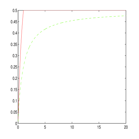
Figure 1: The upper bound $\overline{E}(\rho)/C$ (solid curve) and the lower bound $\underline{E}(\rho)/C$ (dashed curve) for the example of the very noisy channel.

As for the DPT bound, we have the following approximate analysis:

$$e^{-\sup_{q}E(\alpha_{1},\ldots,\alpha_{k},q)} = \inf_{q}\sum_{y\in{\cal Y}}\prod_{i=1}^{k}\left[\sum_{x_{i}\in{\cal X}}q(x_{i})p(y|x_{i})^{\alpha_{i}}\right]$$ (57)

$$= \inf_{q}\sum_{y\in{\cal Y}}\prod_{i=1}^{k}\left\{p(y)^{\alpha_{i}}\left[\sum_{x_{i}\in{\cal X}}q(x_{i})[1+\epsilon(x_{i},y)]^{\alpha_{i}}\right]\right\}$$ (58)

$$= \inf_{q}\sum_{y\in{\cal Y}}p(y)\prod_{i=1}^{k}\left[\sum_{x_{i}\in{\cal X}}q(x_{i})[1+\epsilon(x_{i},y)]^{\alpha_{i}}\right]$$ (59)

$$\approx \inf_{q}\sum_{y\in{\cal Y}}p(y)\prod_{i=1}^{k}\left(\sum_{x_{i}\in{\cal X}}q(x_{i})\left[1+\alpha_{i}\epsilon(x_{i},y)-\frac{1}{2}\alpha_{i}(1-\alpha_{i})\epsilon^{2}(x_{i},y)\right]\right)$$ (60)

$$= \inf_{q}\sum_{y\in{\cal Y}}p(y)\prod_{i=1}^{k}\left[1-\frac{1}{2}\alpha_{i}(1-\alpha_{i})\sum_{x_{i}\in{\cal X}}q(x_{i})\epsilon^{2}(x_{i},y)\right]$$ (61)

$$\approx \inf_{q}\sum_{y\in{\cal Y}}p(y)\left[1-\frac{1}{2}\sum_{i=1}^{k}\alpha_{i}(1-\alpha_{i})\sum_{x_{i}\in{\cal X}}q(x_{i})\epsilon^{2}(x_{i},y)\right]$$ (62)

$$= 1-\frac{1}{2}\sum_{i=1}^{k}\alpha_{i}(1-\alpha_{i})\sup_{q}\sum_{x_{i}\in{\cal X}}\sum_{y\in{\cal Y}}q(x_{i})p(y)\epsilon^{2}(x_{i},y)$$ (63)

$$\approx 1-C\sum_{i=1}^{k}\alpha_{i}(1-\alpha_{i})$$ (64)

$$= 1-C\left(1-\sum_{i=1}^{k}\alpha_{i}^{2}\right).$$ (65)

where in the fifth line, we have used the identity $\sum_{x}q(x)\epsilon(x,y)=0$ for all $y$ with $p(y)>0$ [13, p. 156, eq. (3.4.28)]. Thus,

$$\sup_{q}E(\alpha_{1},\ldots,\alpha_{k},q)=-\ln\left[1-C\left(1-\sum_{i=1}^{k}\alpha_{i}^{2}\right)\right]\approx C\left(1-\sum_{i=1}^{k}\alpha_{i}^{2}\right),$$ (66)

and then

$$\overline{E}_{DPT}(\rho)\approx C\cdot\inf_{k>1}\inf_{\alpha_{1},\ldots,\alpha_{k}}\frac{1-\sum_{i=1}^{k}\alpha_{i}^{2}}{\sum_{i=1}^{k}\zeta_{\rho}(\alpha_{i})}.$$ (67)

The very same expressions are obtained for the continuous–time AWGN channel with unlimited bandwidth, where $C=P/N_{0}$, $P$ being the signal power and $N_{0}$ being the one–sided noise spectral density. For $\rho=1$ and $k=2$, we have $\zeta_{1}(\alpha)=\min\{\alpha,1-\alpha\}$:

$$\overline{E}_{DPT}(1) \leq C\cdot\inf_{0\leq\alpha\leq 1}\frac{1-\alpha^{2}-(1-\alpha)^{2}}{2\min\{\alpha,1-\alpha\}}$$ (68)

$$= C\cdot\inf_{0\leq\alpha\leq 1/2}\frac{2\alpha(1-\alpha)}{2\alpha}=\frac{C}{2},$$ (69)

which agrees with $\overline{E}(\rho)$. For $\rho=2$ and $k=2$, the minimum is attained for $\alpha=1/3$, and the result is $E_{DPT}(2)\leq 8C/9$. However for $k=3$, the bound improves to $C/3$.

6 Extension to the Multidimensional Case

Consider now the case of a parameter vector $\mbox{\boldmath$U$}=(U_{1},\ldots,U_{d})$, uniformly distributed across the unit hypercube $[-1,2,+1/2]^{d}$. A reasonable figure of merit in this case would be a linear combination of $\mbox{\boldmath$E$}\{|\hat{U}_{i}-U_{i}|^{\rho}\}$, $i=1,2,\ldots,d$. Since each one of these terms is exponential in $n$, it makes sense to let the coefficients of this linear combination also be exponential functions of $n$, as otherwise, the results will be exponentially insensitive to the choice of the coefficients. This means that we consider the criterion

$$\sum_{i=1}^{d}e^{nr_{i}}\cdot\mbox{\boldmath$E$}\{|\hat{U}_{i}-U_{i}|^{\rho}\},$$ (70)

where, without loss of generality, we take $r_{i}\geq 0$, $\min_{i}r_{i}=0$.

The derivation below is an extension of the derivation of the channel coding bound, given in Appendix A for the case $d=1$. Therefore, a reader who is interested in the details is advised to read Appendix A first, or otherwise to skip directly to the final result in eq. (87) and the discussion that follows.

Let us define $R_{i}=(r_{i}+\gamma)/\rho$ for some constant $\gamma\geq 0$. Consider the following chain of inequalities:

$$\sum_{i=1}^{d}e^{nr_{i}}\cdot\mbox{\boldmath$E$}\{|\hat{U}_{i}-U_{i}|^{\rho}\} \geq \sum_{i=1}^{d}e^{nr_{i}}\cdot e^{-n\rho R_{i}}\mbox{Pr}\{|\hat{U}_{i}-U_{i}|\geq e^{-nR_{i}}\}$$ (71)

$$= \sum_{i=1}^{d}e^{-n(\rho R_{i}-r_{i})}\mbox{Pr}\{|\hat{U}_{i}-U_{i}|\geq e^{-nR_{i}}\}$$ (72)

$$= e^{-\gamma n}\sum_{i=1}^{d}\mbox{Pr}\{|\hat{U}_{i}-U_{i}|\geq e^{-n(r_{i}+\gamma)/\rho}\}$$ (73)

$$\geq e^{-\gamma n}\cdot\mbox{Pr}\bigcup_{i=1}^{d}\left\{|\hat{U}_{i}-U_{i}|\geq e^{-n(r_{i}+\gamma)/\rho}\right\}$$ (74)

$$\geq e^{-\gamma n}\cdot\exp\left\{-nE_{sl}\left(\frac{1}{\rho}\left[\sum_{i=1}^{d}r_{i}+\gamma d\right]\right)\right\},$$ (75)

where the second line follows from Chebychev’s inequality, the fifth line follows from the union bound, and the last line follows from the same arguments as in [7, Sect. IV.A]. Maximizing over $\gamma$, we get

$$\sum_{i=1}^{d}e^{nr_{i}}\cdot\mbox{\boldmath$E$}\{|\hat{U}_{i}-U_{i}|^{\rho}\}\\ \geq\exp\left\{-n\min_{\gamma\geq 0}\left[\gamma+E_{sl}\left(\frac{1}{\rho}\left[\sum_{i=1}^{d}r_{i}+\gamma d\right]\right)\right]\right\}.$$ (76)

Defining $R=(\sum_{i=1}^{d}r_{i}+\gamma d)/\rho$, $R_{\min}=\sum_{i=1}^{d}r_{i}/\rho$ and $\bar{r}=R_{\min}/d$, the above minimization at the exponent becomes equivalent to

$$\min_{R\geq R_{\min}}\left[\frac{\rho R-\sum_{i}r_{i}}{d}+E_{sl}(R)\right]$$ (77)

$$= \min_{R\geq R_{\min}}\left[\frac{\rho}{d}\cdot R+E_{sl}(R)\right]-\rho\bar{r}$$ (78)

$$= \left\{\begin{array}[]{ll}E_{sp}(R_{\rho/d})+\frac{\rho}{d}(R_{\rho/d}-R_{\min})&\rho/d\leq\rho_{0}\\ E_{ex}(0)-\rho_{0}R_{\min}&\rho/d>\rho_{0}\end{array}\right.$$ (81)

where $R_{\theta}$ is defined as the achiever of $\min_{R\geq R_{\min}}[\theta R+E_{sp}(R)]$. Thus, the extension of the channel–coding bound to the $d$–dimensional case reads

$$\overline{E}(\rho,d,r_{1},\ldots,r_{d}) = \left\{\begin{array}[]{ll}E_{sp}(R_{\rho/d})+\frac{\rho}{d}R_{\rho/d}-\frac{1}{d}\sum_{i=1}^{d}r_{i}&\rho\leq\rho_{0}d\\ E_{ex}(0)-\frac{\rho_{0}}{\rho}\sum_{i=1}^{d}r_{i}&\rho>\rho_{0}d\end{array}\right.$$ (84)

$$= \left\{\begin{array}[]{ll}E_{0}\left(\frac{\rho}{d}\right)-\frac{1}{d}\sum_{i=1}^{d}r_{i}&\rho/d\leq\rho_{0}\\ E_{ex}(0)-\frac{\rho_{0}}{\rho}\sum_{i=1}^{d}r_{i}&\rho/d>\rho_{0}\end{array}\right.$$ (87)

We see that when $r_{i}=0$ for all $i$ (i.e., all weights are 1), it is the same channel–coding bound as before, except that $\rho$ is replaced by $\rho/d$, that is, $\overline{E}(\rho/d)$. For $\rho\to\infty$, the bound tends to $E_{ex}(0)$, which can be approached again by a low–rate code for a Cartesian grid in the parameter space. At the other extreme, when $d$ is very large compared to $\rho$, so $\rho/d$ is small, construct a grid of $e^{n(C-\epsilon)/d}\times e^{n(C-\epsilon)/d}\times\ldots\times e^{n(C-\epsilon)/d}$, quantize $U$ and assign to each grid point a codeword of a typical random code at rate $C-\epsilon$. Then the performance will be about $e^{-n\rho C/d}$. Therefore, as a corollary of the above result, we have

$$\sum_{i=1}^{d}\mbox{\boldmath$E$}\{|\hat{U}_{i}-U_{i}|^{\rho}\}\\ \geq e^{-n[\overline{E}(\rho/d)+o(n)]}.$$ (88)

Appendix A

Proof of Theorem 1. We begin by using the Markov/Chebychev inequality:

$$\mbox{\boldmath$E$}|\hat{U}-U|^{\rho}\geq\Delta^{\rho}\mbox{Pr}\{|\hat{U}-U|\geq\Delta\}.$$ (A.1)

Next we need to further lower bound $\mbox{Pr}\{|\hat{U}-U|\geq\Delta\}$ and then maximize the r.h.s. over $\Delta$. Equivalently, similarly as in [7], we may set $\Delta=e^{-nR}$ in the r.h.s. and maximize the bound w.r.t. $R$. Let $E(R)$ be the reliability function of the channel. Then, similarly as in [7, Theorem 1], we have:

$$\mbox{Pr}\{|\hat{U}-U|\geq e^{-nR}\}\geq e^{-n[E(R)+o(n)]}$$ (A.2)

and so,

$$\mbox{\boldmath$E$}|\hat{U}-U|^{\rho}\geq e^{-n\rho R}\cdot e^{-n[E(R)+o(n)]}=e^{-n[\rho R+E(R)+o(n)]}.$$ (A.3)

The best lower bound is obtained by maximizing the r.h.s. over $R$, yielding

$$\mbox{\boldmath$E$}|\hat{U}-U|^{\rho} \geq e^{-n\min_{R\geq 0}[\rho R+E(R)+o(n)]}$$ (A.4)

$$\geq e^{-n\min_{R\geq 0}[\rho R+E_{sl}(R)+o(n)]}$$

where $E_{sl}(R)$ is the exponent associated with the straight line bound, which is well known to be an upper bound on the reliability function $E(R)$ [9], [10], [13, Sect. 3.8], and which is given by

$$E_{sl}(R)=\left\{\begin{array}[]{ll}E_{ex}(0)-\rho_{0}R&0\leq R\leq R_{0}\\ E_{sp}(R)&R_{0}<R\leq C\\ 0&R>C\end{array}\right.$$ (A.5)

where

$$E_{sp}(R)=\sup_{\varrho\geq 0}[E_{0}(\varrho)-\varrho R]$$ (A.6)

is the sphere–packing exponent, $\rho_{0}$ is as defined in Theorem 1 and $R_{0}$ is the rate $R$ at which $\mbox{d}E_{sp}(R)/\mbox{d}R=-\rho_{0}$, or equivalently, the solution to the equation $E_{sp}(R)=E_{ex}(0)-\rho_{0}R$. Thus, according to the second line of eq. (A.4),

$$\overline{{\cal E}}(\rho)\leq\min_{R\geq 0}[\rho R+E_{sl}(R)].$$ (A.7)

For $\rho\geq\rho_{0}$, the minimum is obviously attained at $R=0$, and so,

$$\overline{{\cal E}}(\rho)\leq\rho\cdot 0+E_{sl}(0)=E_{ex}(0).$$ (A.8)

For $\rho<\rho_{0}$, we use

$$\overline{{\cal E}}(\rho)\leq\min_{R\geq 0}[\rho R+E_{sl}(R)]\leq\min_{R\geq 0}[\rho R+E_{sp}(R)].$$ (A.9)

The right–most side of eq. (A.9) is the Legendre–Fenchel transform (LFT) of $E_{sp}(R)$, which in turn (according to (A.6)), is the LFT of $E_{0}(\rho)$. Thus, the right–most side of (A.9) is given by the UCE of $E_{0}(\rho)$, which is $\overline{E}_{0}(\rho)$. Thus,

$$\overline{{\cal E}}(\rho)\leq\left\{\begin{array}[]{ll}\overline{E}_{0}(\rho)&\rho<\rho_{0}\\ E_{ex}(0)&\rho\geq\rho_{0}\end{array}\right.=\overline{E}(\rho).$$ (A.10)

This completes the proof of Theorem 1.

Appendix B

Proof of Theorem 2. Define

$$R(\rho)=\frac{\underline{E}(\rho)}{\rho}=\left\{\begin{array}[]{ll}\sup_{0\leq\varrho\leq 1}E_{0}(\varrho)/(\varrho+\rho)&\rho\leq\rho_{+}\\ E_{0}(1)/(1+\rho)=E_{x}(1)/(1+\rho)&\rho_{+}<\rho\leq\rho_{-}\\ \sup_{\varrho\geq 1}E_{x}(\varrho)/(\varrho+\rho)&\rho>\rho_{-}\end{array}\right.$$ (B.1)

Consider a grid of $M=e^{nR(\rho)}/2$ evenly spaced points along ${\cal U}$, denoted $\{u_{1},u_{2},\ldots,u_{M}\}$, where $u_{1}=-1/2+e^{-nR(\rho)}$ and $u_{M}=1/2-e^{-nR(\rho)}$ (see also [7, Theorem 2]). If $\rho>\rho_{-}$, assign to each point $u_{i}$ a codeword of a code of rate $R(\rho)$ that achieves the expurgated exponent $E_{ex}[R(\rho)]$. Otherwise, do the same with a code that achieves $E_{r}[R(\rho)]$ (see [4, p. 139, Corollary 1] or [13, Theorem 3.2.1]). Given $u$, let $f_{n}(u)$ be the codeword $\mbox{\boldmath$x$}_{i}$ that is assigned to the grid point $u_{i}$, which is closest to $u$. Given $y$, let $g_{n}(\mbox{\boldmath$y$})$ be the grid point $u_{j}$ that corresponds to the codeword $\mbox{\boldmath$x$}_{j}$ that has been decoded based on $y$ using the ML decoder for the given DMC. For every $R\geq 0$, we have:

$$\mbox{\boldmath$E$}\{|\hat{U}-U|^{\rho}\} = \mbox{\boldmath$E$}\left\{|\hat{U}-U|^{\rho}\bigg{|}|\hat{U}-U|\leq e^{-nR}\right\}\cdot\mbox{Pr}\{|\hat{U}-U|\leq e^{-nR}\}+$$ (B.2)

$$\mbox{\boldmath$E$}\left\{|\hat{U}-U|^{\rho}\bigg{|}|\hat{U}-U|>e^{-nR}\right\}\cdot\mbox{Pr}\{|\hat{U}-U|>e^{-nR}\}$$

$$\leq [e^{-nR}]^{\rho}\cdot 1+1^{\rho}\cdot\mbox{Pr}\{|\hat{U}-U|>e^{-nR}\}$$

$$= e^{-n\rho R}+\mbox{Pr}\{|\hat{U}-U|>e^{-nR}\}.$$

Now, it follows from the construction of the proposed scheme that if $R$ is the coding rate and the spacing between each two consecutive grid points is $2e^{-nR}$, then the event $\{|\hat{U}-U|>e^{-nR}\}$ occurs iff the ML decoder errs. Thus, $\mbox{Pr}\{|\hat{U}-U|>e^{-nR}\}$ is exactly the probability of decoding error. Considering the case $\rho>\rho_{-}$, this code is assumed to achieve the expurgated exponent, and so, this probability of error is upper bounded by $e^{-n\{E_{ex}(R)]-o(n)\}}$. Since $\rho R$ is an increasing function of $R$ and $E_{ex}(R)$ is a decreasing function, the best choice of $R$ is the solution to the equation

$$\rho R=E_{ex}(R)$$ (B.3)

or, equivalently

$$\rho R=\sup_{\varrho\geq 1}[E_{x}(\varrho)-\varrho R].$$ (B.4)

Below we show that the solution to this equation is given by

$$R=R(\rho)\stackrel{{\scriptstyle\Delta}}{{=}}\sup_{\varrho\geq 1}\frac{E_{x}(\varrho)}{\varrho+\rho}$$ (B.5)

and for this choice of $R$, both exponents in the last line of (B.2) are given by

$$\rho R(\rho)=\sup_{\varrho\geq 1}\frac{\rho E_{x}(\varrho)}{\varrho+\rho}$$ (B.6)

which is exactly the expression of $\underline{E}(\rho)$ in the range $\rho>\rho_{-}$. In the range $\rho<\rho_{+}$, exactly the same arguments hold, except that $E_{ex}(R)$ and $E_{x}(\varrho)$ and $\sup_{\varrho\geq 1}$ are replaced by $E_{r}(R)$, $E_{0}(\varrho)$, and $\sup_{0\leq\varrho\leq 1}$, respectively. In the intermediate range, the same line of arguments hold once again, with $\varrho=1$ and $E_{x}(1)\equiv E_{0}(1)$.

It remains to show that $R(\rho)$ in (B.5) solves equation (B.4) for $\rho>\rho_{-}$, and then similar arguments will follow for the two other ranges. Let $R(\rho)$ be defined as in (B.5) and let $R^{\prime}(\rho)$ be defined as the solution to (B.4). We wish to prove that $R(\rho)=R^{\prime}(\rho)$. To this end, we will prove that both $R(\rho)\geq R^{\prime}(\rho)$ and $R(\rho)\leq R^{\prime}(\rho)$. To prove the first inequality, let $\varrho(R)$ denote the achiever of $E_{ex}(R)=\sup_{\varrho\geq 1}[E_{x}(\varrho)-\varrho R]$. Then, by definition of $R^{\prime}(\rho)$, we obviously have

$$\rho R^{\prime}(\rho)=E_{x}[\varrho(R^{\prime}(\rho))]-\varrho[R^{\prime}(\rho)]R^{\prime}(\rho)$$ (B.7)

i.e.,

$$R^{\prime}(\rho)=\frac{E_{x}[\varrho(R^{\prime}(\rho))]}{\varrho[R^{\prime}(\rho)]+\rho}\leq\sup_{\varrho\geq 1}\frac{E_{x}(\varrho)}{\varrho+\rho}\equiv R(\rho).$$ (B.8)

To prove the second (opposite) inequality, let $\varrho(\rho)$ be the achiever of $R(\rho)$, that is,

$$R(\rho)=\frac{E_{x}[\varrho(\rho)]}{\varrho(\rho)+\rho},$$ (B.9)

or, equivalently,

$$\rho R(\rho)=E_{x}[\varrho(\rho)]-\varrho(\rho)R(\rho).$$ (B.10)

But the l.h.s. cannot exceed $\sup_{\varrho\geq 1}[E_{x}(\varrho)-\varrho R(\rho)]=E_{ex}[R(\rho)]$, and so,

$$\rho R(\rho)\leq E_{ex}[R(\rho)].$$ (B.11)

Now, as mentioned earlier, the function $\rho R$ is increasing in $R$ whereas the function $E_{ex}(R)$ is decreasing. Thus, the value of $R$ for which there is equality $\rho R=E_{ex}(R)$, which is $R^{\prime}(\rho)$, cannot be smaller than any value of $R$, for which $\rho R\leq E_{ex}(R)$, like $R(\rho)$. Hence, $R(\rho)\leq R^{\prime}(\rho)$. This completex the proof of Theorem 2.

Appendix C

Derivation of a lower bound on the generalized rate–distortion function. Consider the minimization of the generalized mutual information

$$\tilde{I}(U;\hat{U})=-\mbox{\boldmath$E$}\left\{\int_{{\cal U}}\mbox{d}\hat{u}\prod_{i=1}^{k}p(\hat{u}|U_{i})^{\alpha_{i}}\right\}=-\int_{{\cal U}}\mbox{d}\hat{u}\prod_{i=1}^{k}\int_{{\cal U}}\mbox{d}u_{i}p(u_{i})p(\hat{u}|u_{i})^{\alpha_{i}}.$$ (C.1)

Similarly as in [18, Sect. IV, Example 2] and [6], since we are dealing with an exponentially small estimation error level (small distortion), then for reasons of convenience, we approximate our distortion measure $d(u,\hat{u})=|\hat{u}-u|^{\rho}$ ($u,~{}\hat{u}\in{\cal U}$) by

$$d^{\prime}(u,\hat{u})=|(\hat{u}-u)~{}\mbox{mod}~{}1|^{\rho}.$$ (C.2)

where

$$t~{}\mbox{mod}~{}1\stackrel{{\scriptstyle\Delta}}{{=}}\left<t+\frac{1}{2}\right>-\frac{1}{2}$$ (C.3)

$\left<r\right>$ being the fractional part of $r$, that is, $\left<r\right>=r-\lfloor r\rfloor$. The justification is that for very small distortion (the high–resolution limit), the modulo 1 operation has a negligible effect, and hence $d^{\prime}(u,\hat{u})$ becomes essentially equivalent to the original distortion measure $d(u,\hat{u})=|\hat{u}-u|^{\rho}$. Using the same reasoning as in [18, Sect. IV, Example 2] and [6], there is no loss of optimality by confining attention to channels $p(\hat{u}|u)$ of the form $f(w)$ with $w=\hat{u}-u~{}\mbox{mod}~{}1$. Thus, the minimization of $\tilde{I}(U;\hat{U})$ reduces to the maximization of

$$U(f)=\prod_{i=1}^{k}\mbox{d}w_{i}\int_{-1/2}^{+1/2}\mbox{d}w_{i}[f(w_{i})]^{\alpha_{i}}$$ (C.4)

subject to the constraints

$$\int_{-1/2}^{+1/2}\mbox{d}w\cdot f(w) = 1$$ (C.5)

$$\int_{-1/2}^{+1/2}\mbox{d}w\cdot|w|^{\rho}f(w) = D.$$ (C.6)

This optimization problem is not trivial, but we can find an upper bound on $U(f)$ in terms of $D$ for small $D$. We begin with the following bound for each one of the factors of $U(f)$:

$$\int_{-1/2}^{+1/2}\mbox{d}w\cdot[f(w)]^{\alpha_{i}} = \int_{-1/2}^{+1/2}\mbox{d}w\cdot[f(w)]^{\alpha_{i}}\cdot\left(\frac{|w|^{\rho}+D}{|w|^{\rho}+D}\right)^{\alpha_{i}}$$ (C.7)

$$= \int_{-1/2}^{+1/2}\mbox{d}w\cdot[f(w)(|w|^{\rho}+D)]^{\alpha_{i}}\cdot\left[\frac{1}{(|w|^{\rho}+D)^{\theta_{i}}}\right]^{1-\alpha_{i}}$$ (C.8)

$$\leq \left[\int_{-1/2}^{+1/2}\mbox{d}w\cdot f(w)(|w|^{\rho}+D)\right]^{\alpha_{i}}\cdot\left[\int_{-1/2}^{+1/2}\frac{\mbox{d}w}{(|w|^{\rho}+D)^{\theta_{i}}}\right]^{1-\alpha_{i}}$$ (C.9)

$$= (2D)^{\alpha_{i}}\cdot\left[\int_{-1/2}^{+1/2}\frac{\mbox{d}w}{(|w|^{\rho}+D)^{\theta_{i}}}\right]^{1-\alpha_{i}}.$$ (C.10)

where $\theta_{i}=\alpha_{i}/(1-\alpha_{i})$ and the third line follows from Hölder’s inequality. It remains to evaluate the integral

$$I=\int_{-1/2}^{+1/2}\frac{\mbox{d}w}{(|w|^{\rho}+D)^{\theta_{i}}}.$$ (C.11)

To this end, we have to distinguish between the cases $\theta_{i}>1/\rho$ and $\theta_{i}<1/\rho$ (the case $\theta_{i}=1/\rho$ can be solved separately or approached as a limit of $\theta_{i}\to 1/\rho$ from either side). For the case $\theta_{i}>1/\rho$, letting

$$c_{i}=\int_{-\infty}^{+\infty}\frac{\mbox{d}t}{(|t|^{\rho}+1)^{\theta_{i}}},$$ (C.12)

we can easily bound $I$ as follows:

$$I = D^{-\theta_{i}}\int_{-1/2}^{+1/2}\frac{\mbox{d}w}{(|w/D^{1/\rho}|^{\rho}+1)^{\theta_{i}}}$$ (C.13)

$$\leq D^{1/\rho-\theta_{i}}\int_{-\infty}^{+\infty}\frac{\mbox{d}(w/D^{1/\rho})}{(|w/D^{1/\rho}|^{\rho}+1)^{\theta_{i}}}$$ (C.14)

$$\leq c_{i}D^{1/\rho-\theta_{i}}.$$ (C.15)

For $\theta_{i}<1/\rho$, we proceed as follows:

$$I = D^{1/\rho-\theta_{i}}\int_{-1/(2D^{1/\rho})}^{+1/(2D^{1/\rho})}\frac{\mbox{d}t}{(|t|^{\rho}+1)^{\theta_{i}}}$$ (C.16)

$$= 2D^{1/\rho-\theta_{i}}\int_{0}^{+1/(2D^{1/\rho})}\frac{\mbox{d}t}{(t^{\rho}+1)^{\theta_{i}}}$$ (C.17)

$$\leq 2D^{1/\rho-\theta_{i}}\int_{0}^{+1/(2D^{1/\rho})}\frac{\mbox{d}t}{(\max\{t^{\rho},1\})^{\theta_{i}}}$$ (C.18)

$$= 2D^{1/\rho-\theta_{i}}\int_{0}^{+1/(2D^{1/\rho})}\frac{\mbox{d}t}{\max\{t^{\rho\theta_{i}},1\}}$$ (C.19)

$$= 2D^{1/\rho-\theta_{i}}\left[\int_{0}^{1}\frac{\mbox{d}t}{1}+\int_{1}^{+1/(2D^{1/\rho})}\frac{\mbox{d}t}{t^{\rho\theta_{i}}}\right]$$ (C.20)

$$= 2D^{1/\rho-\theta_{i}}\left[1+\frac{t^{1-\rho\theta_{i}}}{1-\rho\theta_{i}}\bigg{|}_{1}^{1/(2D^{1/\rho})}\right]$$ (C.21)

$$= 2D^{1/\rho-\theta_{i}}\left[1+\frac{2^{\rho\theta_{i}-1}D^{\theta_{i}-1/\rho}-1}{1-\rho\theta_{i}}\right]$$ (C.22)

$$\leq \frac{2^{\rho\theta_{i}}}{1-\rho\theta_{i}}.$$ (C.23)

Thus, defining $c_{i}^{\prime}=2^{\alpha_{i}}\max\{c_{i},2^{\rho\theta_{i}}/(1-\rho\theta_{i})\}$, we have

$$\int_{-1/2}^{+1/2}\mbox{d}w\cdot[f(w)]^{\alpha_{i}} \leq (2D)^{\alpha_{i}}I^{1-\alpha_{i}}$$ (C.24)

$$\leq c_{i}^{\prime}\cdot D^{\zeta_{\rho}(\alpha_{i})},$$ (C.25)

where the function $\zeta_{\rho}(\cdot)$ is defined as in (40). Thus,

$$U(f)\leq c\cdot D^{\sum_{i=1}^{k}\zeta_{\rho}(\alpha_{i})}$$ (C.26)

where $c=\prod_{i=1}^{k}c_{i}^{\prime}$. Finally, it follows that

$$\tilde{R}(D)\geq-c\cdot D^{\sum_{i=1}^{k}\zeta_{\rho}(\alpha_{i})}$$ (C.27)

as claimed.

References

• [1] K. L. Bell, Y. Steinberg, Y. Ephraim, and H. L. van Trees, “Extended Ziv—Zakai lower bounds for vector parameter estimation,” IEEE Trans. Inform. Theory, vol. 43, no. 2, pp. 626–637, March 1997.
• [2] Z. Ben–Haim and Y. C. Eldar, “A lower bound on the Bayesian MSE based on the optimal bias function,” IEEE Trans. Inform. Theory, vol. 55, no. 11, pp. 5179–5196, November 2009.
• [3] D. Chazan, M. Zakai, and J. Ziv, “Improved lower bounds on signal parameter estimation,” IEEE Trans. Inform. Theory, vol. IT–21, no. 1, pp. 90–93, January 1975.
• [4] R. G. Gallager, Information Theory and Reliable Communication, New York, Wiley 1968.
• [5] I. Leibowitz and R. Zamir, “A Ziv–Zakai–Rényi lower bound on distortion at high resolution,” Proc. 2008 IEEE Information Theory Workshop, Porto, Portugal, May 2008.
• [6] N. Merhav, “Data processing inequalities based on a certain structured class of information measures with application to estimation theory,” IEEE Trans. Inform. Theory, vol. 58, no. 8, pp. 5287–5301, August 2012.
• [7] N. Merhav, “On optimum parameter modulation–estimation from a large deviations perspective,” IEEE Trans. Inform. Theory, vol. 58, no. 12, pp. 7215–7225, December 2012.
• [8] A. No, K. Venkat, and T. Weissman, “Joint source–channel coding of one random variable over the Poisson channel,” Proc. ISIT 2012, July 2012.
• [9] C. E. Shannon, R. G. Gallager and E. R. Berlekamp, “ Lower bounds to error probability for coding on discrete memoryless channels. I” Information and Control, vol. 10, pp. 65–103, January 1967.
• [10] C. E. Shannon, R. G. Gallager and E. R. Berlekamp, “ Lower bounds to error probability for coding on discrete memoryless channels. II” Information and Control, vol. 10, pp. 522–552, May 1967.
• [11] S. Tridenski and R. Zamir, “Bounds for joint source–channel coding at high SNR,” Proc. ISIT 2011, pp. 874–878, St. Petersburg, Russia, August 2011.
• [12] H. L. Van Trees and K. L. Bell (Eds), Bayesian Bounds for Parameter Estimation and Nonlinear Filtering/Tracking, IEEE Press, Published by John Wiley & Sons, 2007.
• [13] A. J. Viterbi and J. K. Omura, Principles of Digital Communication and Coding, McGraw–Hill, New York, 1979.
• [14] A. J. Weiss, Fundamental Bounds in Parameter Estimation, Ph.D. dissertation, Tel Aviv University, Tel Aviv, Israel, June 1985.
• [15] J. M. Wozencraft and I. M. Jacobs, Principles of Communication Engineering, John Wiley & Sons, 1965. Reissued by Waveland Press, 1990.
• [16] M. Zakai and J. Ziv, “A generalization of the rate-distortion theory and applications,” in: Information Theory New Trends and Open Problems, edited by G. Longo, Springer-Verlag, 1975, pp. 87–123.
• [17] J. Ziv and M. Zakai, “Some lower bounds on signal parameter estimation,” IEEE Trans. Inform. Theory, vol. IT–15, no. 3, pp. 386–391, May 1969.
• [18] J. Ziv and M. Zakai, “On functionals satisfying a data-processing theorem,” IEEE Trans. Inform. Theory, vol. IT–19, no. 3, pp. 275–283, May 1973.