Fidelity, Rosen-Zener Dynamics, Entropy and Decoherence in one dimensional hard-core bosonic systems

Abstract

We study the non-equilibrium dynamics of a one-dimensional system of hard core bosons (HCBs) in the presence of an onsite potential (with an alternating sign between the odd and even sites) which shows a quantum phase transition (QPT) from the superfluid (SF) phase to the so-called ”Mott Insulator” (MI) phase. The ground state quantum fidelity shows a sharp dip at the quantum critical point (QCP) while the fidelity susceptibility shows a divergence right there with its scaling given in terms of the correlation length exponent of the QPT. We then study the evolution of this bosonic system following a quench in which the magnitude of the alternating potential is changed starting from zero (the SF phase) to a non-zero value (the MI phase) according to a half Rosen Zener (HRZ) scheme or brought back to the initial value following a full Rosen Zener (FRZ) scheme. The local von Neumann entropy density is calculated in the final MI phase (following the HRZ quench) and is found to be less than the equilibrium value ($\log 2$) due to the defects generated in the final state as a result of the quenching starting from the QCP of the system. We also briefly dwell on the FRZ quenching scheme in which the system is finally in the SF phase through the intermediate MI phase and calculate the reduction in the supercurrent and the non-zero value of the residual local entropy density in the final state. Finally, the loss of coherence of a qubit (globally and weekly coupled to the HCB system) which is initially in a pure state is investigated by calculating the time-dependence of the decoherence factor when the HCB chain evolves under a HRZ scheme starting from the SF phase. This result is compared with that of the sudden quench limit of the half Rosen-Zener scheme where an exact analytical form of the decoherence factor can be derived.

1 Introduction

Recent advancements in experiments on ultracold atoms trapped in optical lattices have facilitated the realization of ultracold vapors of bosonic atoms, and hence have opened up new directions towards the experimental studies of low dimensional bosonic systems greiner_prl ; bloch08 . For example, following the pioneering experiments indicating a superfluid (SF) to a Mott insulator (MI) transition in optical lattices in three-dimension greiner02 (and also in one dimension stoferle04 ) and the corresponding study on the non-equilibrium dynamics sadler06 , there is an upsurge in the studies of quantum phase transitions (QPTs) sachdev99 ; chakrabarti96 ; sondhi97 ; continentino ; vojta03 and dynamics of trapped atoms in optical lattices. More interestingly, two dimensional optical lattices have made the quasi one dimensional regime experimentally accessible greiner_prl ; moritz by keeping the transverse potentials much higher than the longitudinal potential. By appropriately tuning the longitudinal potential, different limits of the bosonic Hubbard model have been realized. One of such limits happens to be the hard-core boson (HCB) limit (or the Tonks-Girardeu tonks36 ; lenard66 limit), where two bosons can not occupy the same site; this limit has also been achieved in an optical lattice paredes ; kinoshita . These experiments have paved the way for a plethora of theoretical studies in low-dimensional bosonic systems polkovnikov06 ; cazalilla11 especially from the viewpoint of the SF to the MI transition altman02 ; fischer06 and related non-equilibrium dynamics sengupta04 ; tuchman06 . The HCB systems have turned out to be very advantageous in this context rigol04 ; rousseau06 ; klich07 .

In parallel, there have been numerous studies which attempt to bridge a connection between QPTssachdev99 ; chakrabarti96 ; continentino ; sondhi97 ; vojta03 and quantum information theoretic measures like concurrence osterloh02 ; amico08 , quantum fidelityzanardi06 ; gu10 ; venuti07 ; you07 ; zhou08 ; zhao09 ; gritsev09 ; schwandt09 ; albuquerque10 ; rams11 , quantum discord dillenschneider08 , entanglement entropy vidal03 ; kitaev061 etc.. These measures enable us to detect a QCP and they also show distinctive scaling relations close to it characterized by some of the associated critical exponents. Similarly, the decoherence (or loss of phase information) zurek03 of a qubit coupled to a quantum critical system is also being investigatedrossini07 ; quan06 .

The scaling of the density of defects (or heat) produced following a slow zurek05 ; polkovnikov05 or rapid quenching grandi10 across (or starting from) a QCP has also attracted attention of the scientists. Defects generated in the final state of the quantum system due to the quenching through a QCP in turn lead to non-zero quantum correlations (for example, non-zero local entropy density cherng06 ; mukherjee07 , concurrence sengupta09 , quantum discord nag11 , etc.) in the final state which are otherwise absent in the defect free final state. These information theoretic measures have also been found to satisfy scaling relations identical to that of the defect density in some cases. For recent reviews, see [dutta10 ; polkovnikov11a ; dziarmaga10 ].

In this paper, we study the dynamics of a one-dimensional lattice of HCBs at half-filling in which Bosons are subjected to an onsite potential. The model has a SF long-range order which persists up to a threshold value of the onsite potential at which there is a QPT from the SF to the MI phase which is a chemical potential driven phase transition. Beyond the finite threshold value of the onsite potential (at which a gap opens up in the spectrum) the system becomes an insulator due to correlation effects and we have a Mott insulator in the true sense of the term. We are however interested in the case where the onsite potential is site-dependent (rather, alternates in sign on the even and odd sites); under this condition the SF long-range order is destroyed as soon as the potential is switched on. We put a word of caution here; in our case the site-dependent onsite potential breaks the translation symmetry of the system and any non-zero value of this potential opens up a gap in the spectrum. Though it is not a MI in its true sense we continue to call it so as has been done in literature klich07 . We note that this model has been studied under a (HRZ) quenching scheme rosen32 ; robiscoe78 in which the magnitude of the alternating onsite potential is quenched from zero to a non-zero value and the residual supercurrent in the MI phase has been estimated klich07 .

The motivation of this work is the following: although there has been a series of studies of quantum critical dynamics which involve Landau-Zener tunneling landau (for many examples, see [dutta10 ; polkovnikov11a ; dziarmaga10 ]), the Rosen-Zener (RZ) tunneling (for which the non-adiabatic excitation probability can also be exactly calculated) has received relatively less attention. We use the integrability of the one-dimensional HCB system in an alternating potential along with the exact analytical results for the HRZ quenching to investigate the generation of local entropy in the HCB system in its final MI state following the quench and also the reduction in the supercurrent and residual local entropy in the SF phase following the FRZ quench. We also calculate the decoherence of a qubit connected to the HCB system following a HRZ quenching of the magnitude of the onsite potential. Given the current interest in QPTs, dynamics and quantum information as discussed above, these results are expected to be useful both from experimental and theoretical viewpoints.

The paper is organized in the following way: in Sec. 2, we describe the QPT in the HCB chain in an alternating potential by analyzing the energy spectrum of the Hamiltonian; any non-zero value of the alternating potential leads to an energy gap in an otherwise gapless spectrum so that the system is in the MI phase. In Sec. 3, we show how this QPT can be detected and characterized by investigating the ground state fidelity and fidelity susceptibility.

The dynamics of the HCB chain is studied in Sec. 4. in Sec.4.1, we investigate the single site (local) von Neumann entropy density in the final MI phase following the HRZ quenching for the HCB system. We note that the local entropy density is zero in the SF phase and is equal to $\log 2$ in the MI phase because of its bipartite structure. We, however, find that the value of this entropy in the final MI phase reached after the quenching is less than $\log 2$ by an amount which depends on the parameters of the HRZ quenching. This deviation is due to the fact that the system is quenched out of the SF phase (which is also a gapless QCP) at a finite rate which leads to the defects resulting in a surviving supercurrent and reduced local entropy density in the final MI phase. In Sec.4.2, we study the HCB chain under the full Rosen Zener (FRZ) quenching scheme in which the system is finally brought back to the SF phase through the intermediate MI phase and the surviving supercurrent and the residual local entropy density are calculated.

Finally in Sec.5 a qubit (or a central spin-1/2) is globally coupled to the HCB chain. Our focus is limited to the case when the coupling between the qubit and the HCB chain, which in fact plays the role of an environment to which the qubit is coupled, is very weak. We study the decoherence of the qubit by calculating the decoherence factor in the final state when the onsite potential is changed from zero (the SF phase) to a finite value (the MI phase) following a HRZ quenching scheme in Sec.5.1. An exact expression of the decoherence factor of the qubit is derived analytically in the sudden quench limit in Sec.5.2 where the alternating potential is instantaneously switched on and the results are compared to those of the previous case.

2 The Model

We consider the Lattice-Tonks-Girardeu gas (hard-core) limit of the one-dimensional Bosonic Hubbard model cazalilla11 given by the Hamiltonian

$$\mathcal{H}=-w\sum_{l}(b_{l}^{\dagger}b_{l+1}+\text{h.c})+V\sum_{l}(-1)^{l}b_{l}^{\dagger}b_{l},$$ (1)

where $w$ is the hopping amplitude, $V$ is the onsite potential; $b_{l}$ and $b_{l}^{\dagger}$ are the bosonic annihilation and creation operators at the $l^{th}$ site of the lattice, respectively. These bosonic operators satisfy the canonical commutation relation $[b^{\dagger}_{l},b_{m}]=\delta_{lm}$; additionally, the hard core condition demands, $(b_{l})^{2}=0=(b_{l}^{\dagger})^{2}$. The Hamiltonian (1) undergoes a QPT from the gapless SF phase to the gapped MI phase for any non-zero value of the alternating potential $V$ as shown below.

This Hamiltonian can be exactly solved using Jordan-Wigner (JW) transformationslieb61 given by

$$b_{l}^{\dagger}=\left[\prod_{m<l}\text{exp}\left(a_{m}^{\dagger}a_{m}\right)\right]a_{l}^{\dagger},$$ (2)

where $a_{l}^{\dagger}$ and $a_{l}$ are the JW fermionic operators satisfying the fermion anti-commutation relations $\{a^{\dagger}_{l},a_{m}\}=\delta_{lm},\{a_{l},a_{m}\}=0$. Using JW transformation followed by the Fourier transformation, the energy spectrum of Hamiltonian (1) can be exactly obtained. In terms of JW fermions, the Hamiltonian can be re-written as $\mathcal{H}=\mathcal{H}_{0}+\mathcal{H}_{d}$, where,

$$\begin{split}&\mathcal{H}_{0}=-\sum_{|k|<\pi/2}2w\cos k(a_{k}^{\dagger}a_{k}-a_{k+\pi}^{\dagger}a_{k+\pi}),\\ &\mathcal{H}_{d}=\sum_{|k|<\pi/2}V(a_{k+\pi}^{\dagger}a_{k}+a_{k}^{\dagger}a_{k+\pi}).\end{split}$$ (3)

Evidently, the mode with wave vector $k$ couples to the $(k+\pi)-$ mode, one can rewrite the Hamiltonian in the reduced $2\times 2$ form,

$$\mathcal{H}=\otimes\sum_{|k|<\pi/2}\mathcal{H}_{k},$$ (4)

with

$$\mathcal{H}_{k}=\begin{pmatrix}2w\cos k&-V\\ -V&-2w\cos k\end{pmatrix},$$ (5)

and the energy spectrum (see Fig.(1)) is given by

$$E_{k}=\sqrt{4w^{2}\cos^{2}k+V^{2}}.$$ (6)

We note that the spectrum (6) is gapped even for an infinitesimal alternating potential implying that the system is in the MI phase for any $V\neq 0$. On the other hand, for $V=0$, the spectrum is gapless for the critical mode $k=\pi/2$, and the HCB chain is in the SF phase. It should be noted that the critical modes at $k=\pm\pi/2$ are also the Fermi levels since we are working at half-filling. From the spectrum, we find that the QPT at $V=0$ is characterized by the correlation length exponents $\nu=1$ and the dynamical exponent $z=1$.

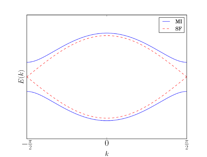
Figure 1: (Color online) The energy spectrum (6) for the model (1) in the reduced Brillouin zone. In the SF phase ($V=0$), the spectrum is gapless at $k=\pi/2$ (red dashed). A non-zero $V$generates a gap in the excitation spectrum at the critical modes are at $k=\pm\pi/2$.

3 Fidelity and Fidelity Susceptibility

One of the most widely used quantum information theoretic measure for detecting and characterizing quantum phase transitions is ground state quantum fidelity gu10 ; venuti07 ; you07 which is the magnitude of the overlap of the two ground states of a quantum many body system belonging to different values of a parameter of the Hamiltonian. Referring to the Hamiltonian (1), we can define quantum fidelity $F(V,V+\delta)$ between two ground states with the alternating potentials $V$ and $V+\delta$, respectively, given by

$$F=|\left<\psi_{0}(V)|\psi_{0}(V+\delta)\right>|=1-\frac{\delta^{2}}{2}L^{d}\chi_{F}+\cdots,$$ (7)

where we have assumed a small system size ($L$) and also $\delta\to 0$ limit, which allow us to truncate the above series at the $\delta^{2}$ order; in the present problem spatial dimensionality $d=1$. The quantity $\chi_{F}=-(2/L^{d})\text{ln}(F)/\delta^{2}|_{\delta\rightarrow 0}$, called the fidelity susceptibility density venuti07 ; you07 ; zhou08 ; zhao09 ; gritsev09 ; schwandt09 ; albuquerque10 ; rams11 , is a measure of the rate of the change of the ground state wave function when the parameter $V$ is changed infinitesimally. Usually quantum fidelity shows a sharp dip at a QCP where $\chi_{F}$ diverges with the system size; the universal scaling of $\chi_{F}$ is given in terms of some of the critical exponents associated with the QPT.

To calculate $F$ and $\chi_{F}$ in the vicinity of the QPT of Hamiltonian (1), we use the reduced two-level Hamiltonian (5). One can use Bogoliubov transformation to obtain the ground state wave function for a particular momentum mode and a given potential $V$ in the form

$$|\psi_{0}(k,V)\rangle=\cos(\theta_{k}(V))|k\rangle+\sin(\theta_{k}(V))|k+\pi\rangle$$ (8)

where $\tan(2\theta_{k}(V))=-{V}/{(2w\cos k)}$. An exact expression of quantum fidelity can be then obtained using Eqs. (7) and (8):

$$F =\prod_{k}|\cos(\theta_{k}(V)-\theta_{k}(V+\delta))|$$

$$=\text{exp}\left[\frac{L}{2\pi}\int_{-\frac{\pi}{2}+\frac{\pi}{L}}^{\frac{\pi}{2}-\frac{\pi}{L}}dk\>\log(|\cos(\theta_{k}(V)-\theta_{k}(V+\delta)|)\right].$$ (9)

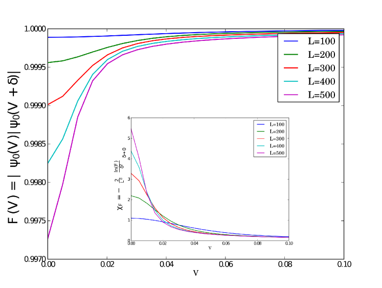
Figure 2: (Color online) Fidelity shows a clear dip at $V=0$. The inset shows that a peak occurs in the fidelity susceptibility at the critical point. Clearly, the value of fidelity drops from unity even away from the QCP as the system size increases.

We also find that $\chi_{F}$ scales as $L$ near $V=0$ (SF phase) and as $V^{-1}$ deep inside MI phase (see Fig.(3)) . Expanding around the critical mode $k=\pi/2$, one arrives at the simplified form

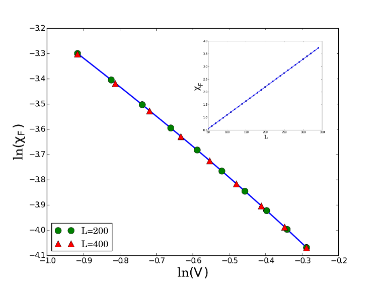
Figure 3: (Color online) Numercially obtained scaling of $\chi_{F}$: away from the QCP, $\chi_{F}\sim V^{-1}$, while in the vicinity QCP, $\chi_{F}\sim L$ (see inset). These scaling relations are in agreement with the theoretical prediction.

$$\begin{split}F=\text{exp}\left[\right.\frac{\delta^{2}}{32\alpha V^{2}}\left\{\right.&\tan^{-1}(\alpha)-\tan^{-1}[\alpha(L-1)]\\ &-\frac{\alpha}{1+\alpha^{2}}+\frac{\alpha(L-1)}{1+\alpha^{2}(L-1)^{2}}\}];\>\>\alpha=\frac{2w\pi}{VL}.\end{split}$$ (10)

The expansion around the critical mode is meaningful because the integrand in the argument of the exponential in Eq.(9) goes to zero near the critical modes. For modes away from the critical mode, the integrand is highly negative and hence their contribution to fidelity is vanishingly small for large $L$. As shown in Fig.(2), the fidelity shows a dip and the susceptibility shows a peak at the QCP, $V=0$. This is in congruence with the generic scalinggritsev09 ; schwandt09 ; albuquerque10 ; rams11 , $\chi_{F}\ \sim L^{2/\nu-d}$ near the QCP ($L\ll V^{-\nu}$), and $\chi_{F}\sim V^{\nu d-2}$ away from the QCP ($L\gg V^{-\nu}$), with $\nu=d=1$.

4 RZ quenching of the on-site potential

In this section, we shall study the HCB model under the HRZ and FRZ quenching schemes and calculate the von Neumann entropy and the diagonal entropy following the HRZ quench and the supercurrent density and the von Neumann entropy following the FRZ quench.

4.1 Von Neumann entropy and Diagonal entropy of the HCB chain following the HRZ quench

In this subsection, we shall employ the HRZ quenching scheme in which the alternating potential is changed from zero to a finite value $V_{0}$, (see Fig. (4)) in a non-linear fashion given by robiscoe78 ; klich07

$$V(t)=\left\{\begin{matrix}V_{0}\left(\text{sech}\left(\frac{\pi t}{\tau}\right)\right)\;\;&t<0\\ V_{0}&t\geq 0.\end{matrix}\right.$$ (11)

This implies that the system is quenched from the SF phase ($t\to-\infty$) to the MI phase ($t=0$).

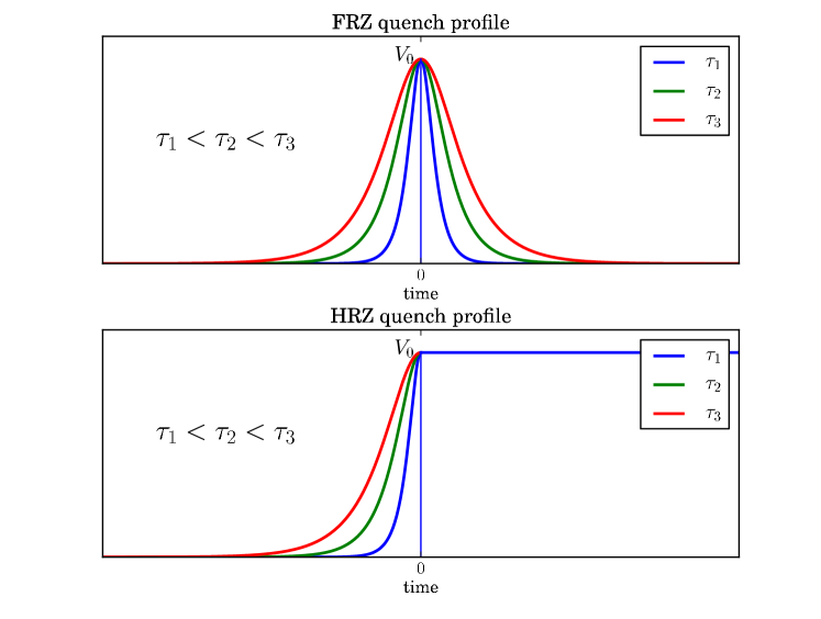
Figure 4: (Color online) The FRZ and HRZ quenching schemes for $V(t)$. We get the sudden quench limit by taking $\tau\rightarrow 0$ in the HRZ case.

In order to calculate the time evolution of $|\psi(t)\rangle$ at a given instant $t$, let us consider a generic state for a given momentum mode: $|\psi_{k}(t)\rangle=s(t)|k\rangle+p(t)|k+\pi\rangle$. Using Schr$\ddot{o}$dinger equations $i\partial|\psi_{k}(t)\rangle/\partial t=\mathcal{H}_{k}|\psi_{k}(t)\rangle$, it can be shown that time evolution of the probability amplitudes $s(t)$ and $p(t)$ are dictated by the equations, klich07 ; rosen32

$$\begin{split}&i\dot{s}(t)=s(t)2w\cos(k)+p(t)V(t),\\ &i\dot{p}(t)=-p(t)2w\cos(k)+s(t)V(t).\end{split}$$ (12)

Using transformations $S(t)=\exp(2iwt\cos{k})s(t)$, $P(t)=\exp(-2iwt\cos{k})p(t)$, we get

$$\begin{split}\ddot{S}=&-\left(\frac{V_{0}}{\text{cosh}\left(\frac{\pi t}{\tau}\right)}\right)^{2}S\\ &+\left[4iw\cos(k)-\frac{\pi}{\tau}\text{tanh}\left(\frac{\pi t}{\tau}\right)\right]\dot{S},\end{split}$$ (13)

which can be reduced to a hypergeometric form with the initial conditions, $|S(-\infty)|=1$ and $|P(-\infty)|=0$. Expanding near the critical mode ($k=\pi/2$), one eventually finds the solution at $t=0$ of the form:

$$\begin{split}&p(0)=-i\sin\left(\frac{V_{0}\tau}{2}\right),\\ &s(0)=\cos\left(\frac{V_{0}\tau}{2}\right).\end{split}$$ (14)

Exploiting the continuity condition of the wave function at $t=0$, let us write the generic wave function for $t>0$ in the form

$$\begin{split}|\psi_{k}(t)\rangle&=c_{g}|g(t)\rangle+c_{e}|e(t)\rangle\\ &=c_{g}e^{iE_{k}t}|g(0)\rangle+c_{e}e^{-iE_{k}t}|e(0)\rangle,\\ \end{split}$$ (15)

where $|g\rangle$ and $|e\rangle$ are the ground state and excited state wave functions (with energies $-E_{k}$ and $E_{k}$) with probability amplitudes $c_{g}$ and $c_{e}$, respectively. Expressing Eq. (LABEL:eq_ge) in terms of momentum modes $|k\rangle$ and $|k+\pi\rangle$ and using Bogoliubov transformation, we get

$$\begin{split}|\psi_{k}(t)\rangle=&(s(0)A_{k}(t)+p(0)B_{k}(t))|k\rangle+\\ &(s(0)B_{k}(t)+p(0)A^{*}_{k}(t))|k+\pi\rangle,\end{split}$$ (16)

where $A_{k}(t)=\cos(E_{k}t)+i\cos(2\theta_{k})\sin(E_{k}t)$, $B_{k}(t)=i\sin(2\theta_{k})\sin(E_{k}t)$ and $E_{k}=\sqrt{4w^{2}\cos^{2}k+V_{0}^{2}}$.

Using the wave function following the quench at an instant $t$ given in Eq. (16), we are now in a position to calculate the single-site von Neumann entropy given by $-\text{Tr}\;\rho\log(\rho)$ where $\rho$ is the density matrix constructed from $|\psi_{k}(t)\rangle$. Ideally in the MI phase, the local von Neumann entropy density $s=\log 2$. (The MI phase is in a pure state and hence the global entropy is zero. However, the (single site) local entropy obtained by integrating over the momentum modes is non-zero because of the bipartite structure of the MI phase. Interpreting in terms of the spin variables, when observed locally upon “coarse-graining” in momentum cherng06 both the spin states appear with an equal probability ($=1/2$) which makes the entropy density $\log 2$ ).

In the present context, however, the MI phase is reached through a non-equilibrium variation of the alternating on-site potential starting from the SF phase at a finite rate and hence the entropy density in the MI phase gets reduced. To calculate it, we decompose the density matrix in a direct product form, $\rho=\bigotimes\prod_{k}\rho_{k}$, where $\rho_{k}$ is the reduced density matrix for the $k$-th mode. Consequently, the entropy density turns to be

$$s=-\frac{1}{\pi}\int_{-\pi/2}^{\pi/2}dk\;\rm{Tr}~{}\rho_{k}\log(\rho_{k})$$ (17)

To calculate $\rho_{k}$ following the HRZ, we use Eq.(16); we are interested in the long-time average of $s$ and since the integrals over $k$ and $t$ commute we can take the long-time average of the terms of $\rho_{k}$ itself before doing the integral over $k$. Taking the long time average of the terms of $\rho_{k}$, we find

$$\rho_{k}=\begin{pmatrix}\frac{\left(1+\cos^{2}2\theta_{k}\cos(V_{0}\tau)\right)}{2}&\frac{\cos 2\theta_{k}\sin 2\theta_{k}\cos(V_{0}\tau)}{2}\\ &\\ \frac{\cos 2\theta_{k}\sin 2\theta_{k}\cos(V_{0}\tau)}{2}&\frac{\left(1-\cos^{2}2\theta_{k}\cos(V_{0}\tau)\right)}{2}\end{pmatrix}.$$ (18)

Diagonalizing the density matrix, the entropy density can be expressed in terms of the eigenvalues $\lambda_{\pm,k}$ as

$$s=-\frac{1}{\pi}\int_{-\pi/2}^{\pi/2}dk\;\lambda_{+,k}\log(\lambda_{+,k})+\lambda_{-,k}\log(\lambda_{-,k}),$$ (19)

where$\lambda_{\pm,k}=\frac{1}{2}\left(1\pm\cos 2\theta_{k}\cos(V_{0}\tau)\right)$. The von Neumann entropy density $s$ increases linearly with $V_{0}$ for $V_{0}<2w$, and saturates to the maximum value of $\log 2$ for higher values of $V_{0}$ (see Fig. (5)). On the other hand, $s$ is found to scale quadratically with $\tau$ (see Fig. (6)). As mentioned already that for a HRZ quenching, the parameters $V_{0}$ and $\tau$ are not on an identical footing which is also reflected in the scaling of $s$.

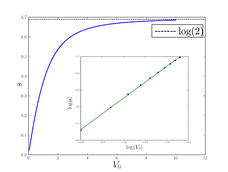
Figure 5: Variation of $s$ with $V_{0}$ in the MI phase (with $w=1$). The inset justifies that $s$ scales linearly with $V_{0}$ for small $V_{0}$.

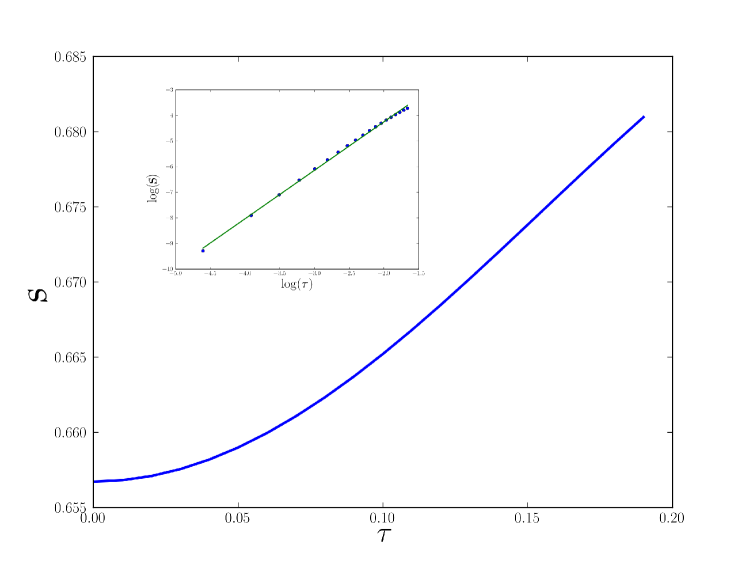
Figure 6: Variation of $s$ with $\tau$ in the MI phase with $w=1$. The inset shows that $\log s$ scales lineally with $\log\tau$ with a slope =2.

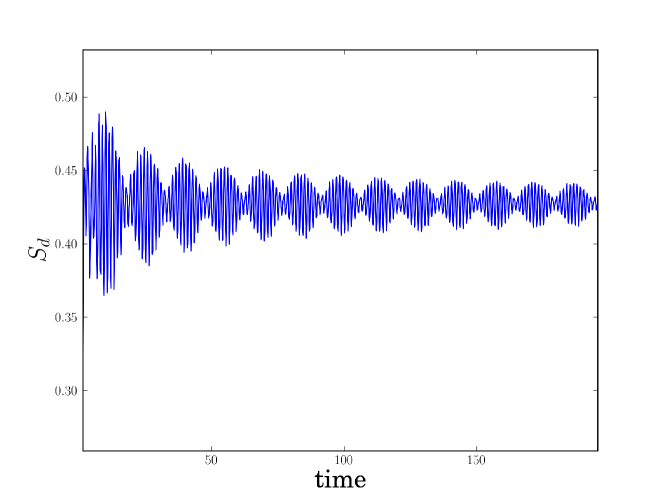
Figure 7: The diagonal entropy density $S_{d}$ is plotted against time shows an oscillatory interference pattern similar to that found in the surviving supercurrent in the MI phase after a similar as reported in klich07 .

One can also calculate the diagonal entropy polkovnikov11b defined as $S_{d}(t)=\sum_{n}\rho_{nn}(t)\log\rho_{nn}(t)$ where $\rho_{nn}(t)$ are the diagonal terms of the density matrix obtained from Eq. (16) (without any time averaging). The diagonal entropy $S_{d}(t)$ shows an oscillatory behavior (see Fig. (7)) similar to the supercurrent in the MI phase following a similar quench klich07 . The scaling of the diagonal entropy $S_{d}$ with $V_{0}$ and $\tau$ is same as compared to the scaling of von Neumann entropy density $s$ in both the region of $V_{0}$.

4.2 Current and von Neumann entropy studies after a FRZ quench

In this subsection, we shall estimate the supercurrent and von Neumann entropy following a FRZ quench of the HCB chain (without the qubit) using the time-evolution of the potential given by the following form:

$$V(t)=V_{0}\>\text{sech}\left(\frac{\pi t}{\tau}\right),\>-\infty<t<+\infty;$$ (20)

the system is initially ($t\to-\infty$) in the SF phase and finally brought back to the SF phase (as $t\to\infty$) through the intermediate MI phase. We study the time evolution of the system after the quenching process gets over (i.e., in the final SF phase). In the SF phase the reduced Hamiltonian is diagonal in the basis $|k\rangle$ and $|k+\pi\rangle$ (with $|k\rangle$ ($|k+\pi\rangle$) being the ground state (excited state)). The wave-function of the HCB system immediately after the FRZ quench (which we set as $t=0$) can be written as a linear combination of these basis states,

$$|\psi(t=0)\rangle=\sqrt{1-P_{k}}|k\rangle+\sqrt{P_{k}}|k+\pi\rangle,$$ (21)

where $P_{k}$ is the RZ non-adiabatic transition formula rosen32

$$P_{k}=\sin^{2}\left(\frac{V_{0}\tau}{2}\right)\text{sech}^{2}[2\tau w\cos{k}].$$ (22)

The time-evolved wave-fuction at some later time $t$ can readily be written as

$$|\psi(t)\rangle=\sqrt{1-P_{k}}e^{-iE_{k}t}|k\rangle+\sqrt{P_{k}}e^{iE_{k}t}|k+\pi\rangle,$$ (23)

where $E_{k}=-2w\cos k$ in the SF phase. In order to calculate supercurrent one has to apply a boost to the Hamiltonian which takes the form $-w\sum_{l}(e^{-i\nu}b_{l}^{\dagger}b_{l+1}+\text{h.c})$ klich07 ; consequently, the momentum value gets shifted from $k$ to $k+\nu$. Expressing the super-current operator, $\hat{j}(t)=\frac{iw}{L}\sum_{l}(e^{-i\nu}b^{\dagger}_{l+1}b_{l}-\text{h.c})$, in the Fourier space, one can find its expectation value with respect to the boosted counterpart of the state (23)

$$j(t) = \frac{w}{\pi}\int_{-\pi/2}^{\pi/2}dk\;\;\;\;\sin(k+\nu)(1-2P_{k+\nu}),$$ (24)

$$= \frac{2w\sin{\nu}}{\pi}\left[1-2\left(V_{0}\tau\right)^{2}\right]$$

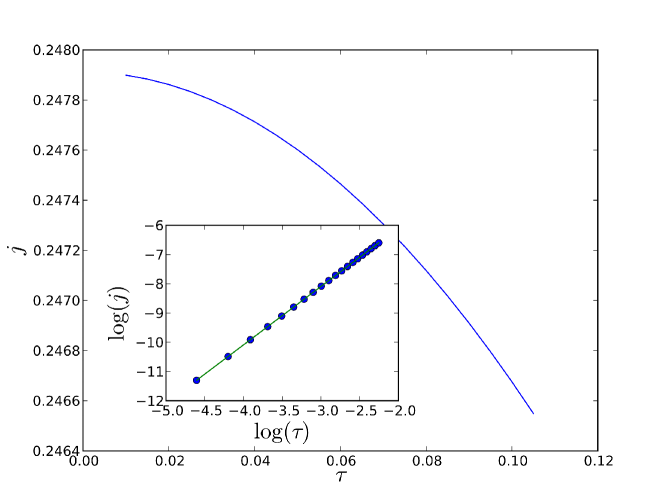
Figure 8: (color online) The figure shows the variation supercurrent $j$ against $\tau$. The inset shows the plot of $\log(j)$ versus $\log(\tau)$, which is a straight line with slope 2

The above result leads the following interesting observations: in the limit of small $\nu$, $\sin(\nu)\sim\nu$, $j\sim\nu$ which is identical to the $\nu$ dependence of the supercurrent in the initial SF phase. Secondly, the supercurrent becomes independent of time after the FRZ quench. This is due to the fact that at the final time HCB system reaches its eigen states. Thirdly, because of the passage through the MI phase starting from a QCP, the current in the final state is reduced from its initial value (at $t\to-\infty$), $(2w\sin\nu/)\pi$, by a factor $V_{0}^{2}\tau^{2}$. It is also to be noted that the the correction term of the supercurrent is a function of the combination $V_{0}\tau$ implying that $V_{0}$ and $\tau$ are on the same footing for the FRZ quenching. This result is numerically verified as shown in Fig. (8).

In a similar spirit, one can calculate the residual von Neumann entropy density in the final SF phase. The rapidly oscillating off-diagonal terms of the reduced density matrix constructed from the wave function given in Eq. (23), vanish over long time averaging cherng06 ; mukherjee07 so that the decohered reduced density matrix has a diagonal form. Calculating the local entropy density using this decohered reduced denstity matrix, one can show that $s\sim V_{0}^{2}\tau^{2}$ (see Fig.(9)). One interesting point should be highlighted here: the quenching through the MI phase generates defects in the SF phase which result in a reduction of the supercurrent and a non-zero value of $s$ both scaling as $V_{o}^{2}\tau^{2}$.

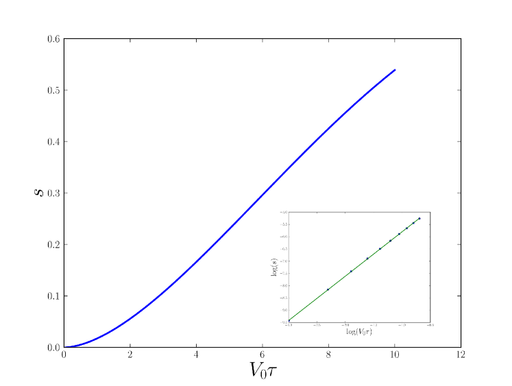
Figure 9: (color online)Variation of $s$ with $V_{0}\tau$ in the SF phase. The inset shows that $s\sim V_{0}^{2}\tau^{2}$ for small $V_{0}$ and $\tau$.

5 Decoherence and HRZ quenching

5.1 Decoherence following a HRZ quencht

In this section, we shall explore the decoherence of a qubit coupled to the environment, chosen to be the HCB chain (1)), which is driven following the HRZ quenching scheme. We assume a global coupling between the qubit and all the bosons of the model (1) with the coupling Hamiltonian given by

$$\mathcal{H}_{\mathcal{SE}}=-\delta\sum_{l}b_{l}^{\dagger}b_{l}\sigma^{z}_{\mathcal{S}},$$ (25)

where $\sigma^{z}_{S}$ represents the qubit, $b_{l}^{\dagger}b_{l}$ is the number density of the environmental HCB chain at site $l$; $\delta$ is the coupling parameter between system and environment. (The form of the coupling Hamiltonian (25) can be interpreted in the following way: the HCB chain can be recast to a transverse XY spin chain in a transverse field in the $z$-direction; the $z$ component of the spin at the site $l$ is coupled to the $z$-component of the central qubit.) In subsequent sections, We shall work in the limit of a weak coupling between the central qubit and HCB system (i.e., $\delta\to 0$).

Due to the coupling to the central qubit, the time evolution of the environmental bosonic chain is split into two channels, corresponding to the $|\left\uparrow\right>(\equiv+1)$ and $|\left\downarrow\right>(\equiv-1)$ state of the the qubit. Using Eq. (5), we find that the reduced Hamiltonians of the HCB system for these two channels, denoted by $\mathcal{H}_{k}^{+}$ and $\mathcal{H}_{k}^{-}$, respectively, are given by

$$\mathcal{H}_{k}^{\pm}=\begin{pmatrix}2w\cos{k}&-(V\pm\delta)\\ -(V\pm\delta)&-2w\cos{k}\end{pmatrix}.$$ (26)

We shall denote the corresponding time-evolved states of the environmental Hamiltonian corresponding to these two branches as $|\psi^{+}(t)\rangle$ and $|\psi^{-}(t)\rangle$, respectively.

One can show that in the limit $\delta\to 0$, the off-diagonal terms of the Hamiltonian(26) can be written as

$$V(t)\pm\delta=V^{\pm}(t)=(V_{0}\pm\delta)\text{sech}\frac{\pi t}{\tau^{\pm}},$$ (27)

where $\tau^{\pm}=\tau\pm\alpha\delta\tau$, with $\alpha$ being a constant of the order of unity. It can be shown numerically that $\alpha$ is not a function of time as well (see Fig.10). It is to be noted that we have made a a small $\tau$ approximation; we intend to study the dynamics close to the sudden quench limit.

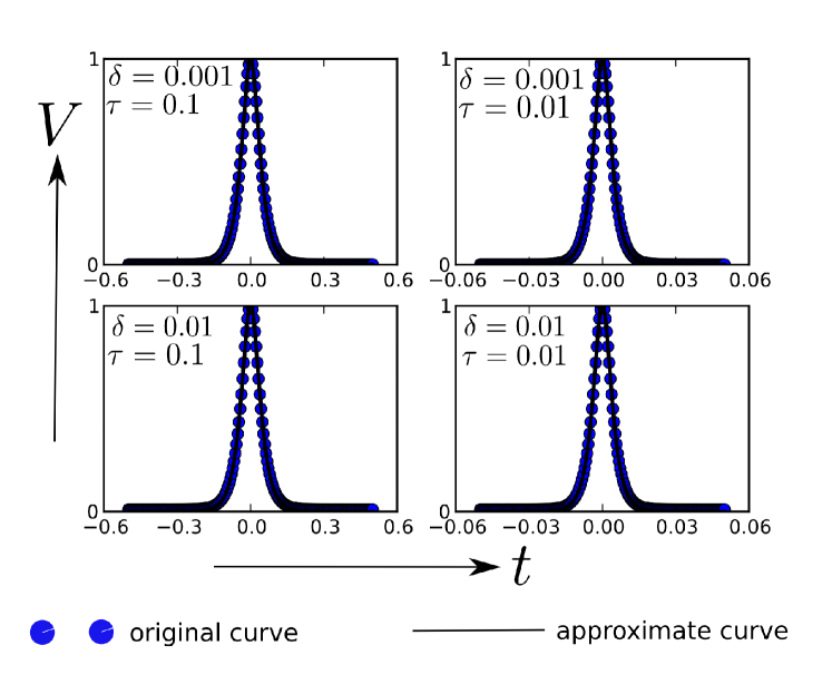
Figure 10: For $\delta\to 0$ and small $\tau$, we verify the approximation made in Eq.(27) by plotting the exact expression and the approximate expression for all time. They are in a very good agreement with each other.

When compared with the RZ form Eq. (11), this approximation implies the following: in the limit of a very weak coupling between the qubit and the environment, the evolution of the two channels can be viewed as two independent HRZ quenches with final potentials and quenching parameters $[(V_{0}+\delta)$, $\tau^{+}]$ and $[(V_{0}-\delta)$, $\tau^{-}]$, respectively.

To study the decoherence of the qubit coupled to the HCB chain following the HRZ quench ($t>0$), one investigates the reduced density matrix of the qubit. We assume that the qubit is initially in a pure state at $t\to-\infty$. The off-diagonal terms of the reduced density matrix for $t>0$ incorporate the decoherence factor $D(t)=|\langle\psi^{+}(t)|\psi^{-}(t)\rangle|^{2}$, which measures the decoherence of the qubit. A non-zero value (less than unity) of $D(t)$ implies that the qubit is in a mixed state and initial phase coherence is lost. Considering the two-level structure of the reduced Hamiltonian of the environmental HCB chain (see (26)) we get,

$$D(t)=\prod_{k}|D_{k}(t)|^{2};~{}~{}~{}~{}D_{k}(t)=|\langle\psi_{k}^{+}(t)|\psi_{k}^{-}(t)\rangle|,$$ (28)

which can be put in the form

$$D(t)=|\langle\psi^{+}(t)|\psi^{-}(t)\rangle|^{2}={\exp}\left(\frac{L}{2\pi}\int_{k=-\pi/2}^{\pi/2}{\ln}(|D_{k}(t)|^{2})dk\right).$$ (29)

To evaluate $D(t)$, we now use Eq. (16) and work in the limit $\delta\to 0$, when one can approximate $\theta^{\pm}_{k}$ (defined after Eq. (8) with $V\to V_{0}\pm\delta$) as

$$\theta^{\pm}_{k}=\theta_{k}+\delta\left.\frac{\partial\theta^{\pm}_{k}}{\partial\delta}\right|_{\delta=0},$$ (30)

where

$$\left.\frac{\partial\theta^{+}_{k}}{\partial\delta}\right|_{\delta=0}=-\left.\frac{\partial\theta^{-}_{k}}{\partial\delta}\right|_{\delta=0}=\frac{-2w\cos k}{4w^{2}\cos^{2}k+V_{0}^{2}}.$$ (31)

One can obtain using Eq. (31)

$$\begin{split}&\langle\psi_{k}^{+}(t)|\psi_{k}^{-}(t)\rangle=\cos(E_{k}^{+}t-E_{k}^{-}t)\cos(2\gamma)+\\ &\sin(E_{k}^{+}t-E_{k}^{-}t)\sin(2\gamma)\left(\sin 2\theta_{k}+2\cos 2\theta_{k}\left.\delta\frac{\partial\theta^{+}_{k}}{\partial\delta}\right|_{\delta=0}\right)-\\ &i\sin(E_{k}^{+}t-E_{k}^{-}t)\cos(2\phi)\left(\cos 2\theta_{k}+2\sin 2\theta_{k}\left.\delta\frac{\partial\theta^{-}_{k}}{\partial\delta}\right|_{\delta=0}\right),\end{split}$$ (32)

where $\gamma=\delta\tau(1+V_{0}\alpha)/2$ and $\phi=V_{0}\tau/2$.

The maximum contribution to the Eq. (32) comes from the modes close to the critical mode $k=\pi/2$. We assume small $\tau$ ($\tau\ll 1$) so that $\delta\tau\to 0$ and use the fact that $\ln(1-x)\sim-x$; the decoherence factor in the early time limit gets reduced to the form

$$\mbox{ln}(|D_{k}(t)|^{2})=-\delta^{2}t^{2}\frac{4V_{0}^{2}}{4w^{2}k^{\prime 2}+V_{0}^{2}}(1+4\tau^{2}w^{2}k^{\prime 2}),$$ (33)

where $k^{\prime}=\pi/2-k$. Using Eq. (33) and Eq. (29) and retaining terms up to the leading orders in $\delta$ and $\tau$, we get

$$\mbox{ln}D(t)=\left[\frac{-L\delta^{2}t^{2}}{2\pi}\left\{\frac{2V_{0}}{w}\tan^{-1}\left(\frac{2\pi w}{V_{0}}\right)\left(1-V_{0}^{2}\tau^{2}\right)+4\pi V_{0}^{2}\tau^{2}\right\}\right].$$ (34)

Eq. (34) is plotted in Fig. (11) which shows a gaussian fall in time of the decoherence factor in the early time limit; this Gaussian fall is the expected behavior in the vicinity of a QCP quan06 .

The scaling of the logarithm of the decoherence factor with $V_{0}$ near the QCP ($V_{0}=0$) is analyzed in the following way; $D(t)$ shows a Gaussian fall in time and is of the form $D(t)\sim e^{-V_{0}^{\lambda}t^{2}}$. We define a quantity $A(V_{0})=-\log D(t)=V_{0}^{\lambda}t^{2}$ and plot $\log A(V_{0})$ versus $\log V_{0}$ for a fixed $t$ (see Fig. (12)). We obtain a straight line whose slope gives us $\lambda$ as $\log A(V_{0})=\lambda\log V_{0}$ for fixed $t$. We find $\lambda=1$ which implies $A\sim V_{0}$. On the other hand, when $V_{0}$ exceed a threshold value (=$2\pi w$), one can expand the $\tan^{-1}$ term in Eq. (34) and show that $D(t)$ is approximately independent of $V_{0}$. Moreover, Fig. (11) also shows that $\log D(t)$ depends very weakly on $\tau$ for $\tau\ll 1$, which is further illustrated in Fig. (12) where we show that curves for different values of $\tau$ fall on top of each other.

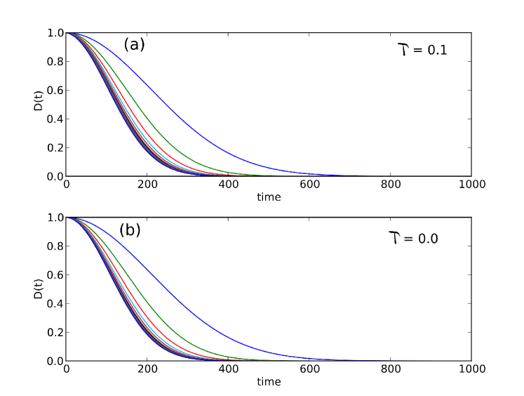
Figure 11: (Color online)(a) Gaussian fall of $D(t)$ following a HRZ quenchis shown with time. The different lines correspond to different values of $V_{0}$. Increasing $V_{0}$ makes the decoherence fall faster. The range of $V_{0}$ covered in the plot is from 1 (blue) to 50 (black). For $V_{0}>2\pi w$, $D(t)$ is approximately independent of $V_{0}$ which is refelcted by the bunching up of the curves for different $V_{0}$ for higher values. (b) The similar nature is observed for $D(t)$ in the sudden quench case ($\tau=0$).

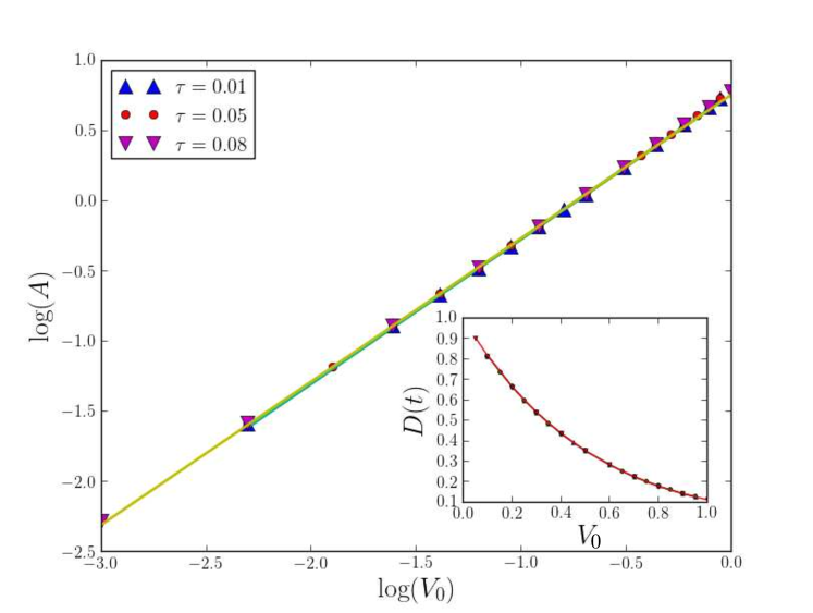
Figure 12: (Color online)Numerically obtained scaling (at fixed $t$): $\log~{}D\sim V_{0}$. It can be seen that the curves for different values of $\tau$ coincide with each other highlighting the weak dependence of $D(t)$ on $\tau$. Inset shows the variation of the decoherence factor of the qubit at a fixed $t$ with $V_{0}$.

5.2 Decoherence in the sudden quench limit

The time evolution of decoherence factor can be derived exactly from the overlap of the initial wave function and the time-evolved version of the final wave function in the sudden quench ($\tau=0$) limit of the HRZ scheme as shown below. In this limit, the onsite the potential is $V=0$ for $t<0$ and it is abruptly changed to $V_{0}+\delta$ (or $V_{0}-\delta$ depending on the initial state of the qubit) at $t=0$. The ground state of the HCB system at $t=0$ is $|\psi(0)\rangle=|k\rangle$, which can be written with the Bogoliubov parameters as

$$|k\rangle=\cos\theta_{k}^{\pm}|g^{\pm}(0)\rangle-\sin\theta_{k}^{\pm}|e^{\pm}(0)\rangle;$$ (35)

Since the ground state and the excited state evolve in time with the corresponding eigenenergies, the wave function for $t>0$ is simply given by

$$|\psi_{k}^{\pm}(t)\rangle=\cos\theta^{\pm}_{k}e^{iE_{k}^{\pm}t}|g^{\pm}(0)\rangle-\sin\theta^{\pm}_{k}e^{-iE_{k}^{\pm}t}|e^{\pm}(0)\rangle.$$ (36)

Expressing $|g^{\pm}(0)\rangle$ and $|e^{\pm}(0)\rangle$ in terms of $|k\rangle$ and $|k+\pi\rangle$ using the Bogoliubov transformations, we find

$$\begin{split}|\psi_{k}^{\pm}(t)\rangle_{SQ}&=|k\rangle[\cos(E_{k}^{\pm}t)+i\sin(E_{k}^{\pm}t)\cos(2\theta_{k}^{\pm})]\\ &+|k+\pi\rangle[i\sin(E_{k}^{\pm}t)\sin(2\theta_{k}^{\pm})],\end{split}$$ (37)

so that using Eq. (37), we find

$$\begin{split}\langle\psi_{k}^{+}(t)&|\psi_{k}^{-}(t)\rangle_{SQ}=\cos(E_{k}^{+}t-E_{k}^{-}t)-\\ &i\left[\sin(E_{k}^{+}t-E_{k}^{-}t)\left\{\cos 2\theta_{k}+2\delta\sin 2\theta_{k}\frac{\partial\theta^{-}_{k}}{\partial\delta}|_{\delta=0}\right\}\right],\end{split}$$ (38)

so that we find

$$\log~{}D(t)=\left[\frac{-L\delta^{2}t^{2}}{2\pi}\left\{\frac{2V_{0}}{w}\tan^{-1}\left(\frac{2\pi w}{V_{0}}\right)\right\}\right].$$ (39)

Comparing Eq. (34) with Eq. (39), we conclude that the decoherence factor for the HRZ quench in the small $\tau$ limit has additional correction terms of the order of $V_{0}^{2}\tau^{2}$. It can also be shown that for $V_{0}/2w>\zeta(\approx 0.75)$, the decay constant dictating the Gaussian decay of the decoherence factor in the early time limit is greater than the sudden quench case in comparison to the HRZ case with small $\tau$.

6 Concluding Comments

In this paper, we have studied the QPT and dynamics of a one dimensional HCB system in the presence of an onsite potential which alternates in sign from site to site. We have shown that the ground state quantum fidelity shows a sharp dip at the QCP ($V=0$) indicating that the system is in the MI phase for any non-zero value of $V$. At the same time the fidelity susceptibility is also found to diverge with the system size in a power-law fashion dictated by the critical exponent $\nu$ (which is unity in the present case).

Subsequently, we have studied the local von Neumann entropy density and diagonal entropy of the HCB chain in MI phase following the HRZ quench starting from the SF phase. The von Neumann entropy density $s$ scales linearly with $V_{0}$ for small values of $V_{0}$ (i.e., $V_{0}<2w$) while it becomes independent of $V_{0}$ for higher values of $V_{0}$. On the other hand, $s$ is found to scale quadratically with $\tau$ throughout. Interestingly, the von Neumann entropy density is found to be less than its expected value of $\log 2$ in the MI phase. This is a consequence of the fact the system is quenched to the MI phase from the SF phase (which is also the QCP) with $s=0$ at a finite rate which leads to defects in the MI phase resulting in a surviving supercurrent klich07 and reduced local entropy.

We have also calculated supercurrent and von Neumann entropy after a FRZ quench when the HCB chain is again brought back to the SF phase; interestingly the reduction in the supercurrent and $s$ both scale identically as ($V_{o}\tau)^{2}$ in the SF phase emphasizing their close connection. It should also be reiterated that following the HRZ quenching there is a surviving supercurrent as well as a reduction in $s$ in the MI phase. On the other hand, for the FRZ scheme it is the other way round; one finds a reduction in supercurrent and a surviving $s$ in the final SF phase.

Finally, we have analyzed the scaling of the decoherence factor $D(t)$ of a central qubit which is globally connected to the HCB system that is driven from the initial SF phase to the MI phase following the HRZ quenching scheme. In the limit of a weak coupling between the qubit and the environmental HCB system and small $\tau$, a threshold value of the magnitude of the alternating potential given by $V_{0}=2\pi w$, is found to exist. Interestingly, the decoherence factor grows linearly with $V_{0}$ when $V_{0}<2\pi w$, whereas for $V_{0}>2\pi w$, it turns to be independent of $V_{0}$. On the other hand, $D(t)$ is found to depend very weekly on the quenching parameter $\tau$. This is due to the fact that the energy spectrum of the Hamiltonian in the MI phase reached through the HRZ quenching scheme depends only on $V_{0}$ and not on $\tau$. In the sudden quench limit ($\tau\to 0$) an exact expression of $D(t)$ is obtained. In the case of a finite but small $\tau$, the decoherence factor, though qualitatively similar to the SQ case, contains additional correction terms (scaling as $(V_{0}\tau)^{2}$). The more interesting observation is that we find the existence of a threshold value of $V_{0}(=1.5w)$, above which there is a faster early time decay of the decoherence factor of the HRZ case for small $\tau$ in comparison to the sudden quenching case. Therefore, above this threshold there is less mixing in the quantum state of the qubit in the sudden quench case as compared to that of the HRZ case.

Acknowledgement

AD acknowledges CSIR, New Delhi for partial support through a project.

References

- (1) Greiner, M., I. Bloch, O. Mandel, T.W. Hänsch and T. Esslinger, Phys. Rev. Lett. 87, 160405, (2001)
- (2) Bloch, I., J. Dalibard and W. Zwerger, Rev. Mod. Phys. 80, 885, (2008).
- (3) Greiner, M., O. Mandel, T. Esslinger, T. W. H änsch, and I. Bloch, Nature (London) 415, 39, (2002)
- (4) Stöferle, T., H. Moritz, C. Schori, M. Köhl, and T. Esslinger, Phys. Rev. Lett. 92, 130403, (2004)
- (5) L. E. Sadler, J. M. Higbie, S. R. Leslie, M. Vengalattore, and D. M. Stamper-Kurn, Nature (London) 443, 312 (2006).
- (6) S. Sachdev, Quantum Phase Transitions (Cambridge University Press, Cambridge, England, 1999).
- (7) B. K. Chakrabarti, A. Dutta, and P. Sen, Quantum Ising Phases and transitions in transverse Ising Models, m41 (Springer, Heidelberg, 1996).
- (8) M. A. Continentino, Quantum Scaling in Many-Body Systems (World Scientific, Singapore, 2001).
- (9) S. L. Sondhi, S. M. Girvin, J. P. Carini, and D. Shahar, Rev. Mod. Phys. 69, 315 (1997).
- (10) M. Vojta, Rep. Prog. Phys. 66, 2069 (2003).
- (11) Moritz, H., T. Stöferle, M. Köhl and T. Esslinger, Phys. Rev. Lett. 91, 250402, (2003)
- (12) L. Tonks, Phys. Rev. 50, 955 (1936); M. Girardeu, J. Math. Phys. (N.Y.) 1, 516 (1960).
- (13) A. Lenard, J. Math. Phys. (N.Y.) 7, 1268 (1966).
- (14) Paredes, B., A. Widera, V. Murg, O. Mandel, S. Fölling, I. Cirac, G. V. Shlyapnikov, T. W. Hänsch, and I. Bloch, Nature 429, 277, (2004)
- (15) Kinoshita, T., T. Wenger, and D. S. Weiss, Science, 305, 1125, (2004)
- (16) Polkovnikov, A., E. Altman, and E. Demler, Proc. Natl. Acad. Sci. USA 103, 6125, (2006).
- (17) M. A. Cazalilla, R. Citro, T. Giamarchi, E. Orignac, and M. Rigol Rev. Mod. Phys. 83, 1405 (2011).
- (18) E. Altman and A. Auerbach, Phys. Rev. Lett. 89, 250404 (2002); A. Polkovnikov, S. Sachdev, and S. M. Girvin, Phys. Rev. A 66, 053607 (2002).
- (19) R. Schützhold, M. Uhlmann, Y. Zu, and U. R. Fischer, Phys. Rev. Lett. 97, 200601 (2006).
- (20) K. Sengupta, S. Powell, and S. Sachdev, Phys. Rev. A 69, 053616 (2004).
- (21) A. K. Tuchman, C. Orzel, A. Polkovnikov, and M. A. Kasevich, Phys. Rev. A 74, 051601 (2006).
- (22) M. Rigol and A. Muramatsu, Phys. Rev. A 70, 031603(R) (2004); ibid 72, 013604 (2005).
- (23) V. G. Rousseau, D. P. Arovas, M. Rigol, F. Hébert, G. G. Batrouni, and R. T. Scalettar, Phys. Rev. B 73, 174516 (2006).
- (24) I. Klich, C. Lannert, and G. Refael, Phys. Rev. Lett. 99, 205303 (2007).
- (25) A. Osterloh, L. Amico, G. Falci, and R. Fazio, Nature 416, 608 (2002); T. J. Osborne and M. A. Nielsen, Phys. Rev. A 66, 032110 (2002).
- (26) L. Amico, R. Fazio, A. Osterloh, V. Vedral, Rev. Mod. Phys. 80, 517-576 (2008).
- (27) P. Zanardi and N. Paunkovic, Phys. Rev. E 74, 031123 (2006).
- (28) S. J. Gu, Int. J. Mod. Phys. B, 24, 4371 (2010).
- (29) L. C. Venuti and P. Zanardi, Phys. Rev. Lett. 99, 095701 (2007), P. Zanardi, P. Giorda, and M. Cozzini, Phys. Rev. Lett. 99, 100603 (2007).
- (30) W.-L. You, Y.-W. Li, and S.-J. Gu, Phys. Rev. E 76, 022101 (2007),S. Yang, S.-L. Gu, C.-P. Sun, and H.-Q. Lin, Phys. Rev. A 78, 012304 (2008).
- (31) H.-Q. Zhou, R. Ors, and G. Vidal, Phys. Rev. Lett. 100, 080601 (2008), H. Zhou and J. P. Barjaktarevic, J. Phys. A, 41 412001 (2008), H.-Q. Zhou, J. H. Zhao, and B. Li, J. Phys. A 41, 492002 (2008).
- (32) J.-H. Zhao and H.-Q. Zhou, Phys. Rev. B 80, 014403 (2009).
- (33) V. Gritsev and A. Polkovnikov, arXiv:0910.3692 (2009), published in Understanding Quantum Phase Transitions, edited by L. D. Carr (Taylor and Francis, Boca Raton, 2010).
- (34) D. Schwandt, F. Alet, and S. Capponi, Phys. Rev. Lett. 103, 170501 (2009).
- (35) A. Fabricio Albuquerque, Fabien Alet, Clement Sire, and Sylvain Capponi, Phys. Rev. B 81, 064418 (2010)
- (36) M. M. Rams and B. Damski, Phys. Rev. Lett. 106, 055701 (2011); M. M. Rams and B. Damski, Phys. Rev. A 84 032324 (2011).
- (37) R. Dillenschneider, Phys. Rev. B 78, 224413 (2008); S. Luo, Phys. Rev. A 77, 042303 (2008); M. S. Sarandy, Phys. Rev. A 80, 022108 (2009).
- (38) G. Vidal, J. I. Latorre, E. Rico, and A. Kitaev, Phys. Rev. Lett. 90, 227902 (2003).
- (39) A. Kitaev and J. Preskill, Phys. Rev. Lett. 96, 110404 (2006).
- (40) W. H. Zurek, Rev. Mod. Phys. 75, 715 (2003); E. Joos, ,Decoherence and appearance of a classical world in a quantum theory (Springer Press, Berlin) (2003), B. Damski, T. Quan and H. Zurek, Phys. Rev. A 83, 062104 (2011);T. Nag, U Divakaran and A. Dutta, Phys. Rev. B 86 (R), 020401 (2012); V. Mukherjee, S. Sharma and A. Dutta, Phys. Rev. B 86, 020301 (R) (2012).
- (41) D. Rossini, T. Calarco, V. Giovannetti, S. Montangero, and R. Fazio, Phys. Rev. A 75, 032333 (2007)
- (42) H. T. Quan, Z. Song, X. F. Liu, P. Zanardi, and C. P. Sun, Phys. Rev. Lett. 96, 140604 (2006).
- (43) W. H. Zurek, et al, Phys. Rev. Lett. 95, 105701 (2005).
- (44) A. Polkovnikov, Phys. Rev. B 72, 161201(R) (2005).
- (45) C. De Grandi, V. Gritsev, and A. Polkovnikov, Phys. Rev. B 81, 012303 (2010); C. De Grandi, V. Gritsev, and A. Polkovnikov, Phys. Rev. B 81, 224301 (2010).
- (46) R. W. Cherng and L.S. Levitov, Phys. Rev. A 73, 043614 (2006).
- (47) V. Mukherjee, U. Divakaran, A. Dutta, and D. Sen, Phys. Rev. B 76, 174303 (2007).
- (48) K. Sengupta, D. Sen, Phys. Rev. A 80, 032304 (2009).
- (49) T. Nag, A. Patra, and A. Dutta, J. Stat. Mech. (2011) P08026.
- (50) A. Dutta, U. Divakaran, D. Sen, B. K. Chakrabarti, T. F. Rosenbaum, and G. Aeppli, arXiv:1012.0653.
- (51) A. Polkovnikov, K. Sengupta, A. Silva, and M. Vengalattore, Rev. Mod. Phys., 83, 863 (2011).
- (52) J. Dziarmaga, Advances in Physics 59, 1063 (2010).
- (53) N. Rosen and C. Zener, Phys. Rev. 40, 502 (1932).
- (54) R. T. Robiscoe, Phys. Rev. A 17, 247–260 (1978).
- (55) C. Zener, Proc. Roy. Soc. London Ser A 137, 696 (1932); L. D. Landau and E. M. Lifshitz, Quantum Mechanics: Non-relativistic Theory, 2nd ed. (Pergamon Press, Oxford, 1965).
- (56) E. Lieb, T. Schultz, and D. Mattis, Annals of Physics, 16, 407 (1961)
- (57) A. Polkovnikov, Annals of Physics, 326, 486 (2011).