Scalar Field Cosmology – Improving the Cosmological Evolutional Scenario

We study evolution of cosmological models filled with the scalar field and barotropic matter. We consider the scalar field minimally and non-minimally coupled to gravity. We demonstrated the growth of degree of complexity of evolutional scenario through the description of matter content in terms of the scalar field. In study of all evolutional paths for all initial conditions methods of dynamical systems are used. Using linearized solutions we present simple method of derivation corresponding form of the Hubble function of the scale factor $H(a)$.

The scalar fields play important role during the cosmic evolution. They are relevant in very early (quantum cosmology, inflation ) as well as late stages of evolution of the Universe (quintessence idea). We study the significance of scalar fields which are additionally non-minimally coupled to gravity in the phase of accelerated expansion of the Universe. For this aims we adopt the methods of dynamical systems which offers possibility of global investigation all evolutional paths for all admissible initial conditions.

We assume the Friedmann-Robertson-Walker (FRW) universe with an arbitrary curvature filled with the non-minimally coupled scalar field and barotropic fluid with the equation of state coefficient $w_{m}$. The action integral is

$$S=\frac{1}{2\kappa^{2}}\int\mathrm{d}^{4}x\sqrt{-g}R-\frac{1}{2}\int\mathrm{d}^{4}x\sqrt{-g}\Big{(}\varepsilon\nabla^{\alpha}\phi\,\nabla_{\alpha}\phi+\varepsilon\xi R\phi^{2}+2U(\phi)\Big{)}+S_{m}$$ (1)

where $\kappa^{2}=8\pi G$, $\varepsilon=\pm 1$ corresponds to canonical and phantom scalar fields, respectively, $R=6\big{(}\dot{H}+2H^{2}+k/a^{2}\big{)}$ is the Ricci curvature scalar, and

$$U(\phi)=U_{0}\big{(}\phi^{2}-\phi_{0}^{2}\big{)}^{2}$$

is the assumed form of the Higgs potential function. $S_{m}$ is the action for the barotropic matter content. From the Einstein equations we obtain the following forms of the energy conservation condition

$$\frac{3}{\kappa^{2}}\left(H^{2}+\frac{k}{a^{2}}\right)=\varepsilon\frac{1}{2}\dot{\phi}^{2}+U(\phi)+\varepsilon 6\xi H\phi\dot{\phi}+\varepsilon 3\xi\phi^{2}\left(H^{2}+\frac{k}{a^{2}}\right)+\rho_{m}\,,$$ (2)

and the acceleration equation

$$\left(1-\varepsilon\xi(1-6\xi)\kappa^{2}\phi^{2}\right)\dot{H} = \frac{k}{a^{2}}-\frac{\kappa^{2}}{2}\bigg{[}\varepsilon(1-2\xi)\dot{\phi}^{2}+\varepsilon 8\xi H\phi\dot{\phi}+2\xi\phi U^{\prime}(\phi)$$ (3)

$$+\varepsilon 2\xi(1+6\xi)\phi^{2}\frac{k}{a^{2}}+\varepsilon 24\xi^{2}\phi^{2}H^{2}+\rho_{m}(1+w_{m})\bigg{]}\,.$$

In what follows we introduce the energy phase space variables $x\equiv\frac{\kappa\dot{\phi}}{\sqrt{6}H}$, $y\equiv\frac{\sqrt{12\,U_{0}}}{\kappa}\frac{1}{H}$, $z\equiv\frac{\kappa}{\sqrt{6}}\phi$, in which the energy conservation condition (2) and the acceleration equation (3) are

$$\Omega_{m}=1-\left[y^{2}(z^{2}-z_{0}^{2})^{2}+\varepsilon(1-6\xi)x^{2}+\varepsilon 6\xi(x+z)^{2}+(1-\varepsilon 6\xi z^{2})\Omega_{k}\right]$$ (4)

$$\left(1-\varepsilon 6\xi(1-6\xi)z^{2}\right)\frac{\dot{H}}{H^{2}} = -\left(1-\varepsilon 6\xi(1+6\xi)z^{2}-\frac{3}{2}(1+w_{m})\left(1-\varepsilon 6\xi z^{2}\right)\right)\Omega_{k}$$ (5)

$$-\varepsilon\frac{3}{2}(1-w_{m})(1-6\xi)x^{2}-\varepsilon 3\xi(1-3w_{m})(x+z)^{2}+\varepsilon 12\xi(1-6\xi)z^{2}$$

$$-\frac{3}{2}(1+wm)\left(1-y^{2}(z^{2}-z_{0}^{2})^{2}\right)-12\xi y^{2}z^{2}(z^{2}-z_{0}^{2})$$

where $\Omega_{m}=\frac{\kappa^{2}\rho_{m}}{3H^{2}}$ and $\Omega_{k}=-\frac{k}{a^{2}H^{2}}$.

Figure 1: The phase space portrait for the flat ($k=0$) FRW model filled with the minimally coupled canonical scalar field ($\varepsilon=+1$, $\xi=0$) and the Higgs potential function $U(\phi)=U_{0}\big{(}\phi^{2}-\phi_{0}^{2}\big{)}^{2}$ and barotropic dust matter ($w_{m}=0$). The critical points correspond to the matter domination and transient acceleration epochs. All trajectories asymptotically approach critical points located at $x^{*}=0$, $y^{*}=\infty$ and $z^{*}=\pm z_{0}$ which corresponds to the Einstein universe with $H^{2}\to 0$.

The dynamics of the model is completely described by the $4$-dimensional dynamical system in variables $x$, $y$, $z$ and $\Omega_{k}$

$$x^{\prime} = -2\left(1-\varepsilon 6\xi(1-6\xi)z^{2}\right)\left(x+3\xi z+\varepsilon y^{2}z(z^{2}-z_{0}^{2})\right)$$ (6)

$$-(x+6\xi z)\bigg{[}1+\varepsilon 6\xi(1-6\xi)z^{2}-\varepsilon\frac{3}{2}(1-w_{m})(1-6\xi)x^{2}-\varepsilon 3\xi(1-3w_{m})(x+z)^{2}$$

$$\hskip 56.9055pt-\frac{3}{2}(1+w_{m})(1-y^{2}(z^{2}-z_{0}^{2})^{2})-12\xi y^{2}z^{2}(z^{2}-z_{0}^{2})\bigg{]}$$

$$+\frac{1}{2}(x+6\xi z)(1-3w_{m})(1-\varepsilon 6\xi z^{2})\Omega_{k}-x(1-\varepsilon 6\xi(1-6\xi)z^{2})\Omega_{k}\,$$

$$y^{\prime} = y\bigg{[}\big{(}1-\varepsilon 6\xi(1+6\xi)z^{2}-\frac{3}{2}(1+w_{m})(1-\varepsilon 6\xi z^{2})\big{)}\Omega_{k}+\varepsilon\frac{3}{2}(1-w_{m})(1-6\xi)x^{2}$$ (7)

$$\hskip 14.22636pt+\varepsilon 3\xi(1-3w_{m})(x+z)^{2}-\varepsilon 12\xi(1-6\xi)z^{2}+\frac{3}{2}(1+w_{m})\big{(}1-y^{2}(z^{2}-z_{0}^{2})^{2}\big{)}$$

$$\hskip 14.22636pt+12\xi y^{2}z^{2}(z^{2}-z_{0}^{2})\bigg{]}\,$$

$$z^{\prime} = x\left(1-\varepsilon 6\xi(1-6\xi)z^{2}\right)\,,$$ (8)

$$\Omega_{k}^{\prime} = 2\Omega_{k}\bigg{[}\big{(}1-\varepsilon 6\xi(1+6\xi)z^{2}-\frac{3}{2}(1+w_{m})(1-\varepsilon 6\xi z^{2})\big{)}\Omega_{k}+\varepsilon\frac{3}{2}(1-w_{m})(1-6\xi)x^{2}$$ (9)

$$\hskip 14.22636pt+\varepsilon 3\xi(1-3w_{m})(x+z)^{2}-1-\varepsilon 6\xi(1-6\xi)z^{2}+\frac{3}{2}(1+w_{m})\big{(}1-y^{2}(z^{2}-z_{0}^{2})^{2}\big{)}$$

$$\hskip 14.22636pt+12\xi y^{2}z^{2}(z^{2}-z_{0}^{2})\bigg{]}$$

where the differentiation is with respect to time $\tau$ defined as $\frac{\mathrm{d}}{\mathrm{d}\tau}=\left(1-\varepsilon 6\xi(1-6\xi)z^{2}\right)\frac{\mathrm{d}}{\mathrm{d}\ln{a}}$. On figures 1 and 2 we present the phase space portraits for the special cases of the minimally ($\xi=0$) coupled scalar fields, both, canonical ($\varepsilon=+1$) and phantom ($\varepsilon=-1$). The dynamics of non-minimally coupled scalar fields is different because of the coupling between the Ricci curvature scalar and the scalar field $\!{}^{{\bf?},{\bf?}}$.

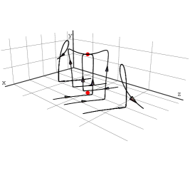
Figure 2: The phase space portrait for the flat ($k=0$) FRW model filled with the minimally coupled phantom scalar field ($\varepsilon=-1$, $\xi=0$) and the Higgs potential function $U(\phi)=U_{0}\big{(}\phi^{2}-\phi_{0}^{2}\big{)}^{2}$ and barotropic dust matter ($w_{m}=0$). The red dots denote critical points of the system and correspond to matter domination and accelerated expansion epochs.

In what follows we concentrate on the single critical point which corresponds to the accelerated expansion of the universe, namely the critical point located at ($x^{*}=0$, $y^{*}=1/z_{0}^{2}$, $z^{*}=0$, $\Omega_{k}^{*}=0$). Using the linearised solution in the vicinity of this point we will show that the solution form of the Hubble function corresponds to the $\Lambda$CDM model independent of the values of the $\xi$ and $z_{0}$ parameters.

Using the energy phase space variable $y\equiv\frac{\sqrt{12\,U_{0}}}{\kappa}\frac{1}{H}$ we can write that

$$\frac{H^{2}}{H_{0}^{2}}=\frac{y(a_{0})^{2}}{y(a)^{2}}$$ (10)

where $H_{0}$ and $y(a_{0})$ are the present time values. Only the linearised solution of the variable $y(\tau)$ is needed in derivation of the Hubble function. It is in the following form

$$y(\tau)=y^{*}+\frac{1}{2z_{0}^{2}}\big{(}2z_{0}^{2}\Delta y+\Delta\Omega_{k}\big{)}\,\,e^{-3(1+w_{m})\tau}-\frac{1}{2z_{0}^{2}}\Delta\Omega_{k}\,\,e^{-2\tau}\,,$$ (11)

where $\Delta y=y^{*}-y^{(i)}$ and $\Delta\Omega_{k}=\Omega_{k}^{*}-\Omega_{k}^{(i)}$ are the initial conditions. Up to linear terms we have $z(\tau)^{2}\approx 0$, then we obtain that the time $\tau$ transforms in to the scale factor as follows $\tau\approx\ln{(\frac{a}{a^{(i)}})}$ where $a^{(i)}$ is the initial value of the scale factor. Finally

$$\frac{y(a_{0})^{2}}{y(a)^{2}} \approx 1+(2z_{0}^{2}\Delta y+\Delta\Omega_{k})\left(\frac{a_{0}}{a^{(i)}}\right)^{-3(1+w_{m})}-\Delta\Omega_{k}\left(\frac{a_{0}}{a^{(i)}}\right)^{-2}$$ (12)

$$-(2z_{0}^{2}\Delta y+\Delta\Omega_{k})\left(\frac{a}{a^{(i)}}\right)^{-3(1+w_{m})}+\Delta\Omega_{k}\left(\frac{a}{a^{(i)}}\right)^{-2}.$$

From the energy conservation condition up to linear terms we have $\Omega_{m,i}\approx-(2z_{0}^{2}\Delta y+\Delta\Omega_{k})$ hence we obtain

$$\frac{H^{2}}{H_{0}^{2}}=1-\Omega_{m,0}-\Omega_{k,0}+\Omega_{m,0}\left(\frac{a}{a_{0}}\right)^{-3(1+w_{m})}+\Omega_{k,0}\left(\frac{a}{a_{0}}\right)^{-2}$$ (13)

which for the dust matter $w_{m}=0$ represents the $\Lambda$CDM model with the curvature.

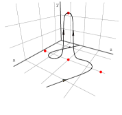
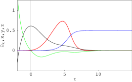
Figure 3: The evolution described by the system of equations (6–9) with $\xi=1/4$ and $z_{0}^{2}=2$. On the left panel we present the projection of $4$-dimensional phase space on the $3$-dimensional subspace ($x$, $y$, $z$) and on the right panel we present time evolution of the phase space variables: $\Omega_{k}(\tau)$ – red, $x(\tau)$ – green, $y(\tau)$ – blue, $z(\tau)$ – black. The sample trajectories interpolate between three major epochs in the history of the universe: the radiation dominated universe, the barotropic matter and finally the quintessence domination epoch.

The dynamics of the scalar field with non-minimal coupling to gravity was studied in details for the Higgs potential of the scalar fields in the framework of dynamical systems methods. We construct 3-dimensional phase portraits for flat and non-flat cosmological models. It is additionally assumed the presence of barotropic matter in the model which gives rise to a new evolutional scenario and enlarges a degree of complexity of cosmic evolution. The structure of phase space was investigated. From the linearization of the system around the critical points we obtain the crucial formula for $H^{2}$ which demonstrated how the standard cosmological model emerges from the model under consideration.

References

References

• [1] O.Β Hrycyna and M.Β Szydlowski, Twister quintessence scenario, Phys. Lett. B694 (2010) 191–197, [arXiv:0906.0335].
• [2] O.Β Hrycyna and M.Β Szydlowski, Uniting cosmological epochs through the twister solution in cosmology with non-minimal coupling, JCAP 12 (2010) 016, [arXiv:1008.1432].