Relativistic rotation curve for cosmological structures

Abstract

Using a general relativistic exact model for spherical structures in a cosmological background, we have put forward an algorithm to calculate the test particle geodesics within such cosmological structures in order to obtain the velocity profile of stars or galaxies. The rotation curve thus obtained is based on a density profile and is independent of any mass definition which is not unique in general relativity. It is then shown that this general relativistic rotation curves for a toy model and a NFW density profile are almost identical to the corresponding Newtonian one, although the general relativistic masses may be quite different.

I Introduction

There has been recently many attempts to understand fully the consistency of the linearized Einstein equations; in other words how far we are right in using Newtonian versus general relativistic gravity in astrophysical and cosmological applications (see for example relativity-newtonian and wald ). We face this controversy in this paper by calculating the general relativistic rotation curve for a spherical structure within a FRW universe. The exact solution gives us the possibility to see if and in which sense the Newtonian approximation is valid in the case of the weak gravity.
The relativistic rotation curve has been the subject of some recent papers (see Cooperstock1 and Cooperstock2 ). The model discussed in these papers, however, is based on the simple Schwarzschild metric, dust collapse, or a simple axially symmetric space-time with a singularity at the central plane, not taking into account the full dynamics of a cosmological structure. We, however, look for an exact solution of Einstein equations representing a cosmological structure as an overdensity region within a cosmological background assumed to be asymptotically FRW. There are not much viable exact models representing such a structure. We will use an analytical model proposed recently based on an inhomogeneous cosmological LTB solution javad1 . Its time-like geodesics are then integrated numerically to obtain the rotation curve of the cosmological structure. Obviously we need a specified density profile for our cosmological structure to obtain the rotation curve, without a need of specifying a mass. In the Newtonian case this is identical to have a unique mass of the structure. In general relativity, however, there is no unique mass definition for astrophysical objects given a specific density profilejavad2 . Therefore, relying on a density profile which is an observational quantity, the non-uniqueness of the concept of mass does not disturb our conclusion about the comparison of the Newtonian versus general relativistic rotation curve.

Section II is a brief introduction to the LTB metric, followed by definitions of some quasi-local masses. In section III we introduce an algorithm how to calculate the rotation curve for a test particle motion around a cosmological structure within a FRW universe. Section IV is devoted to the calculation of the general relativistic rotation curve for a cosmological structure using this algorithm and to compare the results with the Newtonian case. Some general relativistic quasi-local masses are also calculated and compared to the corresponding Newtonian one for the same density profile. We then conclude in section V. Throughout the paper we assume $8\pi G=c=1$.

II LTB model of a structure

The LTB metric in synchronous coordinates is written as

$$ds^{2}=-dt^{2}+\frac{R^{\prime 2}}{1+f(r)}dr^{2}+R(r,t)^{2}d\Omega^{2},$$ (1)

representing a pressure-less perfect fluid satisfying

$$\rho(r,t)=\frac{2M^{\prime}(r)}{R^{2}R^{\prime}},\hskip 22.76228pt\dot{R}^{2}=f+\frac{2M}{R}.$$ (2)

Here dot and prime denote partial derivatives with respect to the parameters $t$ and $r$ respectively. The angular distance $R$, depending on the value of $f$, is given by

$$R=-\frac{M}{f}(1-\cos\eta(r,t)),$$

$$\hskip 22.76228pt\eta-\sin\eta=\frac{(-f)^{3/2}}{M}(t-t_{b}(r)),$$ (3)

for $f<0$, and

$$R=(\frac{9}{2}M)^{\frac{1}{3}}(t-t_{b})^{\frac{2}{3}},$$ (4)

for $f=0$, and

$$R=\frac{M}{f}(\cosh\eta(r,t)-1),$$

$$\hskip 22.76228pt\sinh\eta-\eta=\frac{f^{3/2}}{M}(t-t_{b}(r)),$$ (5)

for $f>0$.
The metric is covariant under the rescaling $r\rightarrow\tilde{r}(r)$. Therefore, one can fix one of the three free functions of the metric, i.e. $t_{b}(r)$, $f(r)$, or $M(r)$. The function $M(r)$ corresponds to the Misner-Sharp mass in general relativity (mis-sha , see also javad2 ). The $r$ dependence of the bang time $t_{b}(r)$ corresponds to a non-simultaneous big-bang or big-crunch singularity.
There are two generic singularities of this metric, where the Kretschmann and Ricci scalars become infinite: the shell focusing singularity at $R(t,r)=0$, and the shell crossing one at $R^{\prime}(t,r)=0$. However, there may occur that in the case of $R(t,r)=0$ the density $\rho=\frac{M^{\prime}}{R^{2}R^{\prime}}$ and the term $\frac{M}{R^{3}}$ remain finite. In this case the Kretschmann scalar remains finite and there is no shell focusing singularity. Similarly, if in the case of vanishing $R^{\prime}$ the term $\frac{M^{\prime}}{R^{\prime}}$ is finite, then the density remains finite and there is no shell crossing singularity either (see javad1 for more detail).
For our model structure, depending on our model calculation, we arrive in the case of a toy model at a specific density profile, or specify a density profile like the NFW one from the beginning. In each case there is a unique Newtonian mass. However, in the relativistic case we may allocate different masses without any preference. Although this does not change our aim of a comparison between the relativistic rotation curve and the Newtonian one, we prefer to show how different these masses may be. Note that the observational quantity is the density profile and not the total mass which is a derived quantity. In fact more than 10 general relativistic mass definitions have already been proposed in the literature. The difference between some of the proposed quasi-local mass definitions has been studied in javad2 , where it has been shown that in the case of spherically symmetric structures the Hawking quasi-local mass is equal to the Misner-sharp one. The Brown-York mass for the 2-boundary specified by $r=constant$ and $t=constant$ ($M_{BY.r}$) in an asymptotically FRW solution is given by

$$M_{BY.r}=-R\sqrt{1+f}+(R\sqrt{1+f})\mid_{FRW}.$$ (6)

If we specify the 2-boundary by $R(r,t)=costant$ and $t=constant$ with $R$ being the areal radius, then the Brown-York mass ($M_{BY.R}$) is given by

$$M_{BY.R}=-R\sqrt{1+\frac{2M}{R}}+(R\sqrt{1+\frac{2M}{R}})\mid_{FRW}.$$ (7)

The Liu-Ya and Epp masses are equal in our spherically symmetric case and are given by

$$M_{LY}=M_{Epp}=-R\sqrt{1+\frac{2M}{R}}+(R\sqrt{1+\frac{2M}{R}})\mid_{FRW}.$$ (8)

We therefore concentrate on three mass definitions: the Misner-Sharp one which is equal to that of Hawking; The Epp mass being equal to Liu-Yau and the Brown-York mass at either the constant areal radius ($R=constant$) or the constant comoving radius ($r=constant$).

III Constructing the model

The model we are going to construct and study should describe a simple model of a spherically symmetric mass condensation within a FRW universe as an exact solution of Einstein equations with a pressure-less ideal fluid. Therefore we will choose a density profile reflecting an overdensity at the center and almost constant density far from the center as expected for a FRW universe. Within such a model structure we then study timelike geodesics to extract information about the rotation curve in such a dynamical setting. This is achieved by specifying the three LTB functions $t_{b}(r)$, $f(r)$, and $M(r)$. Assuming an expanding universe, this cosmic LTB model structure starts expanding with the universe before its expansion decouple from the universe and a collapsing phase starts. There are different ways to specify the LTB functions depending on our needs or our methodology. Once the solution is fixed we may study the timelike geodesics to extract the rotation curve within the structure. Now, the geodesic equations for the LTB metric are given by

$$\frac{d^{2}r}{d{\lambda}^{2}}=\frac{R(1+f)}{R^{\prime}}[\sin(\theta)^{2}({\frac{d\phi}{d{\lambda}}})^{2}+({\frac{d\theta}{d{\lambda}}})^{2}]-\frac{[R^{\prime}R^{\prime\prime}-\frac{{R^{\prime}}^{2}f^{\prime}}{2(1+f)}]}{{R^{\prime}}^{2}}{({\frac{dr}{d{\lambda}}})^{2}}-2\frac{\dot{R^{\prime}}}{R^{\prime}}{({\frac{dt}{d{\lambda}}})({\frac{dr}{d{\lambda}}})},$$ (9)

$${\frac{d^{2}\theta}{d{\lambda}^{2}}=\sin(\theta)\cos(\theta)({\frac{d\phi}{d{\lambda}}})^{2}-2\frac{R^{\prime}}{R}({\frac{dr}{d{\lambda}}})({\frac{d\theta}{d{\lambda}}})-2\frac{R^{\prime}}{R}({\frac{dt}{d{\lambda}}})({\frac{d\theta}{d{\lambda}}})},$$ (10)

$$\frac{d^{2}\phi}{d{\lambda}^{2}}=-2\frac{\cos(\theta)}{\sin(\theta)}(\frac{d\theta}{d{\lambda}})(\frac{d\phi}{d{\lambda}})-2\frac{R^{\prime}}{R}(\frac{dr}{d{\lambda}})(\frac{d\phi}{d{\lambda}})-2\frac{R^{\prime}}{R}(\frac{dt}{d{\lambda}})(\frac{d\phi}{d{\lambda}})$$ (11)

and

$$\frac{d^{2}t}{d{\lambda}^{2}}=-{R{\dot{R}}{\sin(\theta)}^{2}({\frac{d\phi}{d{\lambda}}})^{2}}-R\dot{R}({\frac{d\theta}{d{\lambda}}})^{2}-\frac{R^{\prime}\dot{R^{\prime}}}{1+f}({\frac{dr}{d{\lambda}}})^{2}.$$ (12)

These equations can be simplified by choosing the particle rotation plane in the $\theta=\pi/2$ and by the assumption of the geodesic being time like:

$$-1=-(\frac{dt}{d\lambda})^{2}+\frac{R^{\prime 2}}{1+f}(\frac{dr}{d\lambda})^{2}+R^{2}(\frac{d\theta}{d\lambda})^{2}+R^{2}\sin^{2}(\theta)(\frac{d\phi}{d\lambda})^{2}.$$

Using these geodesic equations, we are able to find dynamical properties of a test particle within this structure. Given that our cosmic structure is dynamic we choose the initial conditions such that the structure is in its late dynamic phase, where the time scale of the evolution of the structure is greater than the time of revolution of the circular path of a test particle. Therefore, we may expect to have quasi-circular geodesics. These are defined either as those having a vanishing radial velocity and acceleration respect to areal radius at the initial conditions, or have an almost constant radius within the numerical precision for a finite angular displacement. We have checked both procedures leading to the same numerical result. Although we have calculated the particle path, its velocity and the rotation curve at distances far from the center using general relativity, it is obvious that these local results should be well within the Newtonian approximation. Now, using the following Newtonian relation, we may define the Newtonian mass corresponding to the structure leading to the circular velocity reflected in the geodesic equations:

$$M_{N}(R)={R}^{2}[{R}{(\frac{d\phi}{d\lambda})}^{2}-\frac{{d}^{2}R}{d{\lambda}^{2}}].$$ (13)

where $R$ is the areal radius with $\lambda$ its affine parameter, and the acceleration given by

$$\frac{{d}^{2}R}{d{\lambda}^{2}}=R^{\prime\prime}(\frac{dr}{d\lambda})^{2}+2{\dot{R^{\prime}}}(\frac{dr}{d\lambda})(\frac{dt}{d\lambda})+R^{\prime}({\frac{d^{2}r}{d{\lambda}^{2}}})+{\ddot{R}}(\frac{dt}{d\lambda})^{2}+\dot{R}(\frac{{d}^{2}t}{d{\lambda}^{2}})$$ (14)

The terms ${\frac{dt}{d\lambda}},\frac{dr}{d\lambda},\frac{d\phi}{d\lambda}$ may be calculated from the geodesic equations.
In addition, we may use any general relativistic mass definition to calculate the relativistic quasi-local mass of the structure. Understanding the difference between these masses and the Newtonian one allocated to the structure and its rotation curve will be the subject of our discussion.

IV Newtonian versus general relativistic rotation curve

We report the results in three steps. To justify our algorithm and the code, we first apply it to the vacuum Schwarzschild case. We then go over to a toy model structure, and finally apply the algorithm to a more realistic case with a NFW density profile.

IV.1 Rotation curve in the vacuum case of Schwarzschild

Noting that the Schwarzschild space-time is a particular case of LTB space-time, we choose the three LTB functions in the following way:

$$f(r)=0,$$ (15)

$$M(r)=m,$$ (16)

$$t_{b}(r)=r.$$ (17)

The resulting Schwarzschild metric is then given by

$$ds^{2}=-dt^{2}+\frac{1}{(\frac{3}{4}m(r-t))^{\frac{2}{3}}}dr^{2}+(2m)^{\frac{2}{3}}(\frac{3}{2}(r-t))^{\frac{4}{3}}({d\theta}^{2}+{sin(\theta)}^{2}{d\phi}^{2}).$$ (18)

This is the metric of the Schwarzschild space-time in a synchronous frame. By studying circular geodesics having vanishing radial acceleration and velocity, we obtain the rotation curve as given in the Fig.(1). Here the mass is the unique Schwarzschild one, which is the same as the Misner-Sharp mass. It is well known that in the case of Schwarzschild space-time at distances far from the center, i.e. $\frac{2M}{R}<<1$, the Misner Sharp mass is equal to all the other general relativistic masses defined so far. Now, to obtain the Newtonian rotation curve we take the Newtonian mass to be equal to the Schwarzschild one and then obtain the corresponding rotation curve. It is seen from Fig.(1) that the relativistic and the Newtonian rotation curves coincide as expected.

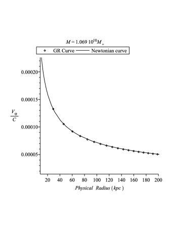
Figure 1: General relativistic and the Newtonian rotation curves for the Schwarzschild metric

IV.2 A toy model

Now we go over to study the rotation curve for a non-trivial but simple toy model. It is constructed as an exact solution of the Einstein equations to represent a cosmic structure within a FRW universe. The three LTB functions are fixed in the following wayjavad1 :

$$M(r)=\frac{{r}^{3/2}\left(1+{r}^{3/2}\right)}{a},\hskip 22.76228pt\ t_{b}(r)=0,\hskip 22.76228pt\ f(r)=-(\frac{r{{\rm e}^{-r}}}{b}).$$ (19)

The model represents a typical galaxy as a cosmological structure showing the formation of a central black hole with distinct event- and apparent horizon. As expected for a cosmological structure, the density profile shows a void before entering the asymptotic FRW region. Fig.(2) shows the density profile of the toy model and its corresponding relativistic and Newtonian rotation curve. The Newtonian rotation curve is calculated using the mass related to the density profile at a specific radius. As we see from the figure, both rotation curves are almost identical.
We note by passing that the density profile is obtained without fixing the mass which is not uniquely defined in general relativity in contrast to the Newtonian case. Therefore, as our algorithm shows, the rotation curve may be uniquely defined once we have fixed the density profile for a specific solution of Einstein equations. In other words, any rotation curve within a cosmological structure corresponds to a unique density profile but not a unique mass, in contrast to the Newtonian case. This is shown in Fig. (3).

 

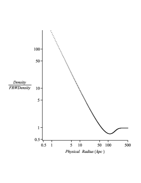
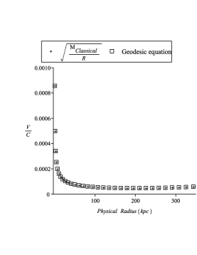
Figure 2: Density profile for the toy model of a typical galaxy and the corresponding general relativistic and Newtonian rotation curve

 

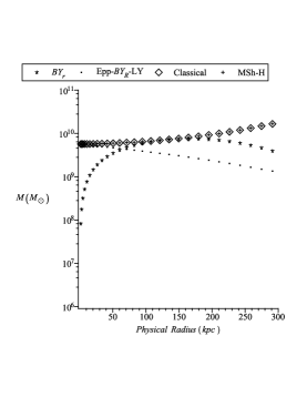
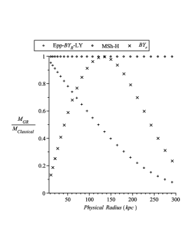
Figure 3: Quasi-local masses for a toy model of a galaxy corresponding to the density profile of the toy model

IV.3 NFW model

Now, we try a model structure with a NFW density profile nfw . This density profile is used to find the areal radius through an algorithm formulated in krasinki , see also javad2 . To use this algorithm, the density profile has to be specified at two different initial and final times, $t_{i},t_{f}$ as a function of the coordinate $r$. Now, the algorithm is based on the choice of $r$-coordinate such that $M(r)=r$. This is due to the fact that $M(r)$ is an increasing function of $r$. Therefore, $E$ and $t_{b}$ become functions of $M$. The LTB functions $E(M)$ and $t_{b}(M)$ may then be extracted from the algorithm. For the initial time we choose the time of the last scattering surface: $t_{i}\simeq 3.77\times 10^{5}yr$. The initial density profile should show a small over-density near the center imitating otherwise a FRW universe. Therefore, we add a Gaussian peak to the FRW background density. We know already that having an over-density in an otherwise homogeneous universe needs a void to compensate for the extra mass within the over-density region. Therefore, to compensate this mass we subtract a wider gaussian peak. These density profiles may then be written as

$$\rho_{i}(r)=\rho_{crit}(t_{i})((\delta_{i}e^{-(\frac{r}{R_{i1}})^{2}}-b_{i})e^{-(\frac{r}{R_{i2}})^{2}}+{1}),$$ (20)

$$\rho_{f}(r)=\rho_{crit}(t_{f})((\frac{\delta_{c}}{(\frac{r}{r_{s}})(1+\frac{r}{r_{s}})^{2}}-b_{f})e^{-(\frac{r}{R_{f}})^{2}}+1),$$ (21)

where $\delta_{i}$ is the density contrast of the Gaussian peak, $R_{i1}$ is the width of the Gaussian peak and $R_{i2}$ is the width of the negative Gaussian profile at the initial time. The two constants $b_{i}$ and $b_{f}$ are then obtained by the mass compensation condition. The results for the NFW density profile of a typical galaxy and the corresponding relativistic and Newtonian rotation curves are given in Fig.(4). We see again that both Newtonian and relativistic rotation curves coincide.
We have also calculated different general relativistic masses to see how different they are, although this does not change our results as far as the rotation curve for a specific density profile is concerned. The results are shown in Fig.(5). As in the case of the toy model, we realize that the Misner-Sharp mass is almost identical to the Newtonian one. There is however substantial difference to other general relativistic masses.

 

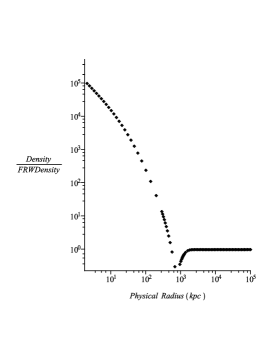
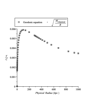
Figure 4: Density profile for the NFW model of a galaxy and the corresponding Newtonian and relativistic rotation curve

 

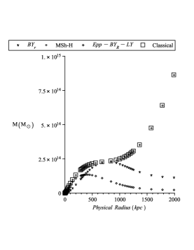
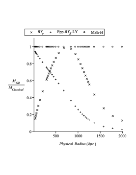
Figure 5: Ratio of GR masses to the Newtonian mass for the NFW density profile of a galaxy

V discussion and conclusion

We have tried for the first time to answer the question of how a relativistic rotation curve for a general relativistic structure within an otherwise expanding universe looks like based on the Einstein equations. To achieve this, we have modeled our so-called cosmological structure using a LTB cosmological solution tending to FRW universe at infinity and having an overdense structure at the center. After the original expansion, the overdense region starts collapsing leading to a dense structure before going over to a FRW universe. The mass in-fall to the structure reduces at late times leading to an almost static structure. This late time behavior gives us the possibility of defining quasi-circular orbits for particles revolving around it.
We have then defined an algorithm how to obtain the relativistic rotation curve for a specific density profile, without relying on a mass definition for the structure which is not unique in general relativity. The numerical procedure is tested first for a Schwarzschild metric where we have shown that it is equivalent to the Newtonian rotation curve. We know already that in this case all the general relativistic masses are equivalent to the Newtonian mass. In the case of a general relativistic cosmological structure we choose first a toy model and then a NFW density profile.
Now, for our cosmological structure which is embedded in a dynamical FRW background, it turns out that the rotation curve at the galactic scale and at far distances from the center of the structure (where the gravity is weak), is almost identical to the Newtonian one, which is the main result of our work. We have also calculated the general relativistic mass definitions for our models to see how different they are, despite having a unique rotation curve due to the specific density profile.

VI ACKNOWLEDGMENT

We would like to thank Mojahed Parsi Mood for helpful discussions and providing us his NFW model data.

References

- (1) S. F. Flender and D. J. Schwarz, Phys. Rev. D 86, 063527 (2012) [arXiv:1207.2035 [astro-ph.CO]]; J. -c. Hwang and H. Noh, Gen. Rel. Grav. 38, 703 (2006) [astro-ph/0512636]; L. Lopez-Honorez, O. Mena and S. Rigolin, Phys. Rev. D 85, 023511 (2012) [arXiv:1109.5117 [astro-ph.CO]].
- (2) Stephen R. Green, Robert M. Wald, Phys. Rev. D 83: 084020, (2011); Stephen R. Green, Robert M. Wald, Phys. Rev. D 85: 063512, (2012).
- (3) J. D. Carrick, F. I. Cooperstock, [arXiv:1101.3224 [astro-ph]].
- (4) F. I. Cooperstock, S. Tieu, Mod. Phys. Lett. A23, 1745-1755 (2008). [arXiv:0712.0019 [astro-ph]].
- (5) J.T. Firouzjaee, Reza Mansouri, Gen. Relativ. Gravit. 42, 2431 (2010), [arXiv:0812.5108]; J.T. Firouzjaee, Int. J. Mod. Phys. D, 21, 1250039 (2012) [arXiv:1102.1062]; Krasinski A. and Hellaby C., Phys. Rev. D69, 043502 (2004); Rahim Moradi, J. T. Firouzjaee, Reza Mansouri, [arXiv:1301.1480].
- (6) J. T. Firouzjaee, M. Parsi Mood and Reza Mansouri, Gen. Relativ. Gravit. 44, 639 (2012) [arXiv:1010.3971]
- (7) Arnowitt R, Deser S and Misner C W 1962 in Gravitation, an Introduction to Current Research ed: Witten L (New York: Wiley)
- (8) Bondi H, van der Burg M G J and Metzner A W K 1962 Proc. Roy. Soc. Lond. A269 21; Sachs R K 1962 Proc. Roy. Soc. Lond. A270 103
- (9) Misner C W and Sharp D H 1964 Phys. Rev. 136 B571.
- (10) J.D. Brown and J.W. York, Jr., Phys. Rev. D 47, 1407- 1419 (1993).
- (11) Hawking S W 1968 J. Math. Phys. 9 598.
- (12) R.J. Epp, Phys. Rev. D 62, 124018 (2000)
- (13) C-C.M. Liu and S-T. Yau, Phys. Rev. Lett. 90, 231102 (2003).
- (14) Classical Dynamics of Particles and Systems,Stephen T. Thornton, Jerry B. Marion,3th Edition,1988
- (15) Hawking S W, J. Math. Phys. 9 598 (1968).
- (16) J.F. Navarro, C.S. Frenk, S.D.M. White, ApJ, 462, 563 (1996).
- (17) A. Krasiński, C. Hellaby, Phys. Rev. D 65, 023501 (2001).