On quantum corrected Kähler potentials in F-theory

Abstract

We work out the exact in $g_{s}$ and perturbatively exact in $\alpha^{\prime}$ result for the vector multiplet moduli Kähler potential in a specific $\mathcal{N}=2$ compactification of F-theory. The well-known $\alpha^{\prime 3}$ correction is absent, but there is a rich structure of corrections at all even orders in $\alpha^{\prime}$. Moreover, each of these orders independently displays an $SL(2,\mathbb{Z})$ invariant set of corrections in the string coupling constant. This generalizes earlier findings to the case of a non-trivial elliptic fibration. Our results pave the way for the analysis of quantum corrections in the more complicated $\mathcal{N}=1$ context, and may have interesting implications for the study of moduli stabilization in string theory.

1 Introduction

In recent years, there has been a resurgence of interest in F-theory Vafa:1996xn . This renewed interest is due largely to the observation that certain realistic particle physics features, such as the gauge group, matter content, and couplings of Grand Unified Theories (GUTs), can be elegantly obtained in this framework Donagi:2008ca ; Beasley:2008dc ; Hayashi:2008ba ; Beasley:2008kw (see Weigand:2010wm ; Maharana:2012tu for recent reviews). Besides extending the D-brane phenomenology program to describe realistic GUTs, another (perhaps the original) appeal of F-theory is that it provides a geometrical way to formulate and analyze type IIB string vacua non-perturbatively.

The power of F-theory lies in its potential to geometrically describe the non-perturbative physics of string theory, but aspects of its effective action obtained so far have not yet fully exploited this property. In lack of an action principle or a microscopic formulation of F-theory, one often has to rely on F-theory as a limit of M-theory to obtain its low energy effective action Dasgupta:1999ss ; Denef:2008wq ; Grimm:2010ks ; Grimm:2011sk ; Grimm:2011fx ; Bonetti:2011mw ; Grimm:2012rg (see Becker:1996gj for the starting M-theory solutions). While geometry and low energy consistency conditions impose constraints on the low energy effective action, the underlying symmetries of type IIB string theory are not always apparent. In this paper, we shall make extensive use of string dualities in order to derive aspects of the quantum corrected effective action of F-theory. In particular, we explore simple F-theory models which admit several dual descriptions (see figure 2 for the web of string dualities involved). The dual descriptions enable one to compute in some cases not only the perturbative $\alpha^{\prime}$ corrections to F-theory, but also results that are fully non-perturbative in the string coupling. In our approach, the non-perturbative $SL(2,{\mathbb{Z}})$ symmetry is manifest in the effective action. The Kähler potential so obtained should generalize fully non-perturbatively the type IIB result.

One of the interesting features of F-theory compactifications is that one may be able to naturally combine phenomenological model construction with moduli stabilization analysis Blumenhagen:2008zz ; Collinucci:2008sq ; Cicoli:2011qg . Given that the leading $\alpha^{\prime}$ corrections to the Kähler potential has played a key role in the so-called LARGE Volume Scenario (LVS) of Balasubramanian:2005zx ; Conlon:2005ki , we expect that our generalization of these type IIB results to F-theory should have some interesting implications to moduli stabilization. In LVS, string corrections to the tree-level supergravity effective action computed in Becker:2002nn play an essential role, and a volume modulus is stabilized so that the compactification volume is as large as $10^{15}$ in string units. Since the scenario relies on the specific string correction of $\mathcal{O}(\alpha^{\prime 3})$ in the string frame to the Kähler potential, other corrections might have some effects on the moduli stabilization. Indeed, some perturbative one-loop $g_{s}$ corrections to some $\mathcal{N}=1$ and $\mathcal{N}=2$ toroidal orientifold models were computed in Berg:2005ja (see also Antoniadis:1996vw ). Ref. Berg:2005ja found corrections of order $\mathcal{O}(g_{s}^{2}\alpha^{\prime 2})$ in the string frame to the Kähler potential. Hence, one has to check which corrections are leading, in order to find a true minimum. Interestingly, there can be certain cancellations for the latter correction in the scalar potential, and some models are robust against the inclusion of the latter correction in a certain region of the moduli space vonGersdorff:2005bf ; Berg:2005yu ; Berg:2007wt ; Cicoli:2007xp . In this respect, one of our aims here is to generalize the result in Berg:2005ja to full $g_{s}$ corrections including non-perturbative terms in $g_{s}$. This is particularly important for F-theory compactifications since typical GUTs require a strong coupling effect in $g_{s}$ for generating some favorable phenomenological features. Although $\mathcal{N}=1$ models are of interest for this purpose, $\mathcal{N}=2$ models will still exhibit interesting structures in the corrections. In fact, the qualitative features of $\mathcal{N}=2$ corrections is similar to the $\mathcal{N}=1$ corrections in toroidal orientifold models considered in Berg:2005ja . As mentioned before, on the other hand, $\mathcal{N}=2$ supersymmetry is powerful enough to obtain fully non-perturbative $g_{s}$ corrections as well as all the perturbative $\alpha^{\prime}$ corrections. Motivated by these observations, we will work on finding the effective action of a particular $\mathcal{N}=2$ F-theory model in this paper.

More precisely, we concentrate on F-theory compactified on K3$\times$K3. We shall be able to disentangle $g_{s}$ and $\alpha^{\prime}$ corrections and discuss the roles played by the various moduli of the two K3 manifolds. In particular, Kähler modulus and complex structure moduli of the elliptic K3, while decoupled at tree-level in $\alpha^{\prime}$, are non-trivially mixed at loop-level. The structure of this mixing is rigidly constrained by the $SL(2,\mathbb{Z})$ invariance of the underlying type IIB theory and we will propose a purely F-theoretic interpretation of this fact coming from the M-theory description of F-theory, generalizing the results for compactifications on trivial elliptic fibrations first found in Green:1997tv ; Green:1997di ; Green:1997as ; Green:1998by .

This paper is organized as follows. In section 2, we discuss some general issues about the effective action of F-theory, and set up the computation of the Kähler potential which we aim to address in this work. In section 3, we review the basics of the string theory model under consideration, focusing on how various supersymmetry multiplets transform and on the duality relations connecting the type IIB model to type I and to heterotic. In section 4, we systematically analyze the threshold corrections to the Kähler metric of the vector multiplet moduli space of type I^′ string (and hence F-)theory, both with and without Wilson lines. We will check explicitly that the Kähler potential to each perturbative order in $\alpha^{\prime}$ is invariant under an $SL(2,{\mathbb{Z}})$ symmetry. In section 5, we provide a geometric, F-theory interpretation of the type IIB result in section 4 by making use of the F/M-theory duality. We shall argue that the threshold corrections to the Kähler potential can be interpreted in F-theory as coming from integrating loops of 11D super gravitons with various momenta. We conclude in section 6. Some important but more technical details are relegated to the appendices.

2 Setting up the problem

We would like to take some steps towards understanding quantum corrections to the Kähler potential of F-theory compactifications. In particular, F-theory already represents a completion of type IIB string theory as far as string-loop corrections are concerned, but it is perturbative with respect to $\alpha^{\prime}$ corrections, exactly on the same footing as type IIB supergravity. This fact is reflected in the basic objects of the effective field theory arising from an F-theory compactification Grimm:2010ks ; Denef:2008wq . For instance, consider F-theory compactified on a smooth, elliptically fibered Calabi-Yau fourfold. At tree level in $\alpha^{\prime}$, the 4d, $\mathcal{N}=1$ Kähler potential splits in two decoupled contributions:

$$\mathcal{K}=\mathcal{K}_{K}+\mathcal{K}_{c}\,,$$ (1)

where the first is due to moduli of the Kähler structure only and the second to moduli of the complex structure only of the internal fourfold. Explicitly they look like:

$$\mathcal{K}_{K}=-3\log\mathcal{V}_{{\rm CY}_{4}}\,,\qquad\qquad\mathcal{K}_{c}=-\log\int_{{\rm CY}_{4}}\Omega_{4}\wedge\bar{\Omega}_{4}\,,$$ (2)

where $\mathcal{V}_{{\rm CY}_{4}}$ is the classical volume of the Calabi-Yau fourfold, while $\Omega_{4}$ is its unique holomorphic $(4,0)$-form. The complex structure moduli of the internal fourfold contain three different kinds of moduli of the underlying type IIB weak coupling orientifold compactification (Sen limit): The bulk moduli of the internal Calabi-Yau threefold (closed string moduli), the 7-brane deformation moduli (open string moduli) and the axio-dilaton $S=C_{0}+ie^{-\phi}$, thought of as an actual 4d modulus. Indeed, generically the complex structure of the torus fiber is not a modulus because it varies over the internal space according to the implicit relation

$$j(S({\bf z}))=\frac{4(24f)^{3}}{27g^{2}+4f^{3}}({\bf z})\,,$$ (3)

where $j$ is the modular invariant Klein function while $f$ and $g$ are polynomial functions of the base coordinates ${\bf z}$, defining the Weierstrass representation of the elliptic fibration. The solution for $S$ of eq. (3) encodes the backreaction on the axiodilaton of a given 7-brane solution of type IIB string theory. However, the Sen parameterization of $f$ and $g$ allows to isolate from the backreacted solution a constant piece $S_{0}$, which represents the asymptotic value of the axiodilaton far away from the 7-brane sources in a given chart, and thus behaves as a true 4d modulus.

In general the computation of the periods of $\Omega_{4}$ to evaluate $\mathcal{K}_{c}$ is extremely hard, and possible only in case one has few moduli. However, to make clear our purposes, it is instructive to consider its weak coupling limit. Taking the Sen limit of an F-theory compactification just means finding a region in the complex structure moduli space of the fourfold in which the imaginary part of the axio-dilaton can be sent to infinity in a globally well-defined way. In doing so one sees that the discriminant of the elliptic fibration gets factorized in two pieces, whose vanishing locus can be interpreted in a suitable $SL(2,\mathbb{Z})$ frame as a D7-brane and an O7-plane. Since now the string coupling constant $g_{s}$ can be kept small everywhere on the base (except on the locus where the O7 sits), one can make a perturbative expansion of $\mathcal{K}_{c}$ in $g_{s}$:

$$\mathcal{K}_{c}=-\log({\rm Im}S_{0})-\log i\int_{{\rm CY}_{3}}\Omega_{3}\wedge\bar{\Omega}_{3}+\frac{g_{s}}{2i\int_{{\rm CY}_{3}}\Omega_{3}\wedge\bar{\Omega}_{3}}\mathcal{K}_{\rm D7}+\mathcal{O}(g_{s}^{2})\,,$$ (4)

where the first two terms are respectively the standard Kähler potentials for the dilaton and for the complex structure moduli of the CY threefold in type IIB string theory. The third term governs the D7-brane moduli and it depends on both open and closed string moduli. Notice that it enters at linear order in $g_{s}$, which means that the backreaction of the D7-branes on the bulk geometry is suppressed by a power of $g_{s}$. Therefore at lowest order in $g_{s}$ no open string moduli appear at all.

From the analysis above one therefore expects that the full $\mathcal{K}_{c}$ in eq. (2) contains all the $g_{s}$ corrections of type IIB string theory, perturbative or not. Moreover, since $\mathcal{K}_{c}$ only depends on the fibration structure of the fourfold, one also expects that the whole set of corrections appears in it in an $SL(2,\mathbb{Z})$ invariant fashion for the complex structure of the fiber. Indeed, in any point of the moduli space, if one applies an overall $SL(2,\mathbb{Z})$ transformation to the corresponding fourfold one does not change its intrinsic fibration structure, but rather one is trivializing each chart of the base in a different way, but all at the same time, so that the transition functions do not change. In other words, over each chart of the base, one is taking a different representative of the complex structure of the torus fiber above that chart, in such a way that the transitions between two intersecting charts do not change. Consequently, one changes the names of all the 7-branes which appears (namely the monodromy that defines them), but their mutual relations are untouched. Of course in the perturbative expansion just described the $SL(2,\mathbb{Z})$ symmetry is explicitly broken by a preferred choice of $SL(2,\mathbb{Z})$-frame (in the weak coupling limit only D7’s and O7’s appear), which allows us to consistently retain only a few orders in $g_{s}$ (neither the monodromy around a D7 nor the one around an O7 contains the ‘S’ generator of $SL(2,\mathbb{Z})$). The essence of section 4 will be to use, in a concrete model, powerful results from heterotic string theory to sum up all $g_{s}$ corrections in type IIB for a given $\alpha^{\prime}$ order. In doing so, each O7-plane is actually resolved in a couple of mutually non-perturbative (p,q)7-branes. Nevertheless our focus will not be on the full backreacted solution $S({\bf z})$, as the latter is a consequence of the intrinsic structure of the F-theory fibration. Rather we will concentrate on the 4d modulus $S_{0}$ and on its $SL(2,\mathbb{Z})$-class. To anticipate the result, we will verify that physical quantities will not depend on the specific representative of that class at every order in $\alpha^{\prime}$. Consequently, the Kähler potential will only be invariant up to Kähler transformations and this is due to the fact that the explicit expression for the Kähler potential is usually written in the covering space of the modulus $S_{0}$, namely the upper half complex plane. Hence the Kähler transformations are changes between patches within the Kähler moduli space induced by the $SL(2,\mathbb{Z})$ transition functions acting on the local coordinate $S_{0}$.

By viewing F-theory as M-theory on the same fourfold upon sending the volume of the fiber to 0 (F-theory limit), one may suspect that the $SL(2,\mathbb{Z})$ invariance of the Kähler potential (up to Kähler transformations) only holds when the CY fourfold is trivially fibered (no 7-branes, thus constant axiodilaton, i.e. $S=S_{0}$). Indeed, in this case ${\rm CY}_{4}={\rm CY}_{3}\times T^{2}$ and $SL(2,\mathbb{Z})$ is now a target space duality of the M-theory background and hence any physical quantity is invariant under this group. This property has been highlighted in the computations of Collinucci:2009nv . However, the geometrical, sketchy argument presented above is not restricted to the trivial case and suggests that this invariance property persists in more general cases.

One can also argue the $SL(2,\mathbb{Z})$ invariance at the level of the Weierstrass form at least for a smooth case. At each point in the base of a smooth elliptically fibered Calabi–Yau fourfold, the defining equation with a section may be written by the Weierstrass form

$$y^{2}=x^{3}+fx+g,$$ (5)

where $f$ and $g$ may be expressed as

$$f=-15\sum_{\omega\in m\omega_{1}+n\omega_{2}}\frac{1}{\omega^{4}},\quad g=-35\sum_{\omega\in m\omega_{1}+n\omega_{2}}\frac{1}{\omega^{6}}.$$ (6)

Here $m$ and $n$ in the sum are integers except for $(m,n)=0$, and $\omega_{1}$ and $\omega_{2}$ are the two periods of the lattice defining the torus. The complex structure $\tau$ of the torus is related to the periods by $\tau=\frac{\omega_{2}}{\omega_{1}}$. Since the sum in (6) is taken for all the periods except for $0$, the $SL(2,\mathbb{Z})$ transformation for $\omega_{1}$ and $\omega_{2}$

$$\omega_{2}^{\prime} = a\omega_{2}+b\omega_{1},$$ (7)

$$\omega_{1}^{\prime} = c\omega_{2}+d\omega_{1}$$ (8)

with $a,b,c,d\in\mathbb{Z}$ and $ad-bc=1$ does not change $f$ and $g$. One can do the same $SL(2,\mathbb{Z})$ transformation at every point in the base of the elliptically fibered Calabi–Yau fourfold. Therefore, the defining equation of the smooth elliptically fibered Calabi–Yau fourfold does not change by the $SL(2,\mathbb{Z})$ transformation. For a singular Calabi–Yau fourfold, we may have 7-branes and also matter fields from the intersection between 7-branes in some singular loci. The gauge fields or matter fields may be realized by string junctions between the 7-branes. The configurations of the string junctions also do not change by the overall $SL(2,\mathbb{Z})$ transformation.

In order to argue the $SL(2,\mathbb{Z})$ invariance at the level of the Kähler potential in a low energy effective field theory, there might be a subtlety if the $SL(2,\mathbb{Z})$ transformation involves a weak–strong coupling transformation. For example, one might not have a local Lagrangian description if the $SL(2,\mathbb{Z})$ transformed theory becomes strongly coupled. However, the gauge couplings of the gauge fields coming from the Kaluza–Klein reduction or the gauge fields on the D7-branes do not change under the $SL(2,\mathbb{Z})$ transformation. For the Kaluza-Klein gauge fields, the kinetic term arises from the dimensional reduction of the ten-dimensional Einstein-Hilbert action in the Einstein frame. Since the metric in the Einstein frame does not change under the $SL(2,\mathbb{Z})$ transformation, the gauge coupling for the Kaluza-Klein gauge fields does not change. For the gauge fields on D7-branes, the gauge coupling is roughly

$$\frac{1}{g_{\text{YM}}^{2}}\sim\frac{\text{Vol(4-cycle)}}{g_{s}},$$ (9)

where the Vol(4-cycle) stands for the string frame volume of the four-cycle which the D7-branes wrap. The expression (9) becomes in the Einstein frame

$$\frac{1}{g_{\text{YM}}^{2}}\sim\frac{\text{Vol(4-cycle)}}{g_{s}}=\widehat{\text{Vol}}(\text{4-cycle}),$$ (10)

where $\widehat{\text{Vol}}(\text{4-cycle})$ represents the Einstein frame volume of the four-cycle. Therefore, the gauge coupling for the gauge fields on the D7-branes does not change under the $SL(2,\mathbb{Z})$ transformation. To summarize, the gauge couplings for the two types of the gauge fields remains to be weak after the $SL(2,\mathbb{Z})$ transformation if the original gauge couplings are weak. Hence, one may safely use the Kähler potentials on both sides and argue the $SL(2,\mathbb{Z})$ invariance of the corresponding Kähler metrics.

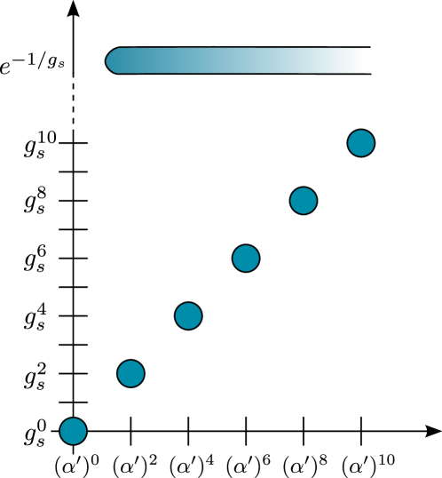
Figure 1: Quantum corrections to the prepotential of F-theory on $K3\times K3$. The horizontal axis labels the degree in $\alpha^{\prime}$ of the correction, and the vertical one the degree in $g_{s}$. The circles represent the non-vanishing perturbative terms in the prepotential. The solid band on top represents the set of non-perturbative corrections in $g_{s}$; Notice that there are no such corrections at tree level in $\alpha^{\prime}$, as discussed in the text.

Moreover we expect that this property still holds at higher order in $\alpha^{\prime}$. Eq. (2) is only the tree-level expression in $\alpha^{\prime}$. At higher $\alpha^{\prime}$-orders, in general, Kähler and complex structure moduli will mix. Nevertheless, since the $SL(2,\mathbb{Z})$ duality of type IIB string theory is believed to hold at all orders in $\alpha^{\prime}$, we expect that, at each $\alpha^{\prime}$-order, there will be a suitable F-theoretic expression depending on geometrical quantities of the internal CY fourfold which contains a sum of all $g_{s}$ corrections in an $SL(2,\mathbb{Z})$ invariant fashion, as $\mathcal{K}_{c}$ in eq. (2) does for the lowest $\alpha^{\prime}$ order. In other words, all kinds of corrections take place in a square (see fig. 1), in which the horizontal line corresponds to $\alpha^{\prime}$ corrections and the vertical to $g_{s}$ ones. Each $\alpha^{\prime}$-tower of corrections to physical quantities should display the $SL(2,\mathbb{Z})$ invariance.

In the following we try to verify the above statements by studying a specific, well known F-theory background, namely F-theory on $K3\times K3$ Sethi:1996es ; Bershadsky:1997ec ; Kakushadze:1998cd ; Lerche:1998nx ; Greene:2000gh ; Gorlich:2004qm ; Lust:2005bd ; Aspinwall:2005ad ; Valandro:2008zg . On the one hand this is more general than in Collinucci:2009nv because it involves a non-trivial fibration (the second $K3$ is elliptically fibered over a 2-sphere). On the other hand, however, this model is particularly well tractable because it leads to an $\mathcal{N}=2$ four-dimensional effective theory which enjoys all the nice non-renormalization theorems for its relevant quantities. In addition, in this case, we have at our disposal a well-studied dual heterotic model, in which corrections have been computed explicitly. This will help us understand systematically the structure of both $\alpha^{\prime}$ and $g_{s}$ corrections, which will turn out to be particularly easy. We will find all our expectations verified and provide a clear picture of the whole duality web of corrections, stating precisely which points of the square in fig. 1 is occupied by a correction, and what is the explicit form of the latter. Notice that the simplification arising in this model is actually a consequence of the $\mathcal{N}=2$ supersymmetry. In $\mathcal{N}=1$ models $\alpha^{\prime}$ and $g_{s}$ corrections might be entangled in an intricate way, which may not allow one to easily isolate the $\alpha^{\prime}$-towers of $g_{s}$ corrections and check their $SL(2,\mathbb{Z})$ invariance.

3 Review of the model

In this section we will review the basics of the string theory model which we want to work with, focusing on the susy representations in which the various low-energy fields transform and on the duality relations connecting the type IIB model to type I and to heterotic. We will not give an extensive treatment, but rather pay attention only to the details we will make use of in the sequel and, in particular, describe the F-theory lift of this model.

3.1 Generalities

We consider the so called type I^′ string theory, namely type IIB compactified on $K3\times T^{2}/\mathbb{Z}_{2}$, where the $\mathbb{Z}_{2}$ quotient is an orientifold, whose geometrical action is just to reflect the coordinates of $T^{2}$. This action has four fixed points which are regarded as the positions of four $O7^{-}$-planes wrapping $\mathbb{R}^{1,3}\times K3$. This compactification leads to an $\mathcal{N}=2$, 4d effective theory, which is the orientifold truncation of an $\mathcal{N}=4$ one. The various moduli fields of the low-energy theory will arrange into vector multiplets and hypermultiplets as follows. The complex structure of $T^{2}$ ($U$), the overall Kähler modulus (volume plus axion) of $K3$ ($T$), the axio-dilaton ($S$) and the transverse positions of the 16 D7-branes ($C^{i}$) which are needed to cancel the 7-brane tadpole are all scalar components of 19 vector multiplets. The complex structure moduli of $K3$ plus the Kähler modulus of $T^{2}$ will instead constitute the scalar fields of a number of hypermultiplets. Note that this is different from the compactifications of Type IIB string theory on Calabi-Yau threefolds where the dilaton is a scalar component of the universal hypermultiplet. This is because Tripathy:2002qw there the vector fields come from the reduction of RR fields in the usual Calabi-Yau threefold compactifications. Hence, the gauge kinetic terms do not have the dilaton dependence. On the other hand, in the present case, there are gauge fields coming from the reduction of $B_{2}$. Therefore, there exists a gauge kinetic term of the form Andrianopoli:2003jf

$$e^{-2\phi_{10}^{I^{\prime}}}\sqrt{G_{4}}\sqrt{G_{T^{2}}}\sqrt{G_{K3}}G^{\mu_{1}\nu_{1}}G^{\mu_{2}\nu_{2}}G^{ij}_{T^{2}}H_{\mu_{1}\mu_{2}i}H_{\nu_{1}\nu_{2}j}.$$ (11)

where $i,j$ are directions of the torus. Then the kinetic term of the gauge fields contain the dilaton $e^{-2\phi_{10}^{I^{\prime}}}$, the volume of $K3$, $\sqrt{G_{K3}}$, and the complex structure of $T^{2}$, $\sqrt{G_{T^{2}}}G^{ij}$. Since the gauge kinetic term in $\mathcal{N}=2$ supersymmetric field theory is written in terms of $\mathcal{N}=2$ vector multiplets, we conclude that $S_{I^{\prime}},T_{I^{\prime}},U_{I^{\prime}}$ are scalar components of vector multiplets.

Our main interest here is to study corrections to the metric of the vector multiplet moduli space, which is a Special Kähler manifold. Hence all we need is the prepotential as a function of our 19 moduli. Due to its holomorphicity property, quantum corrections to the prepotential are very well under control and this constitutes an enormous simplification in carrying out our analysis.

This type IIB model has also the advantage of admitting a chain of dualities to other type of string theories. Indeed, type I^′ string theory can be obtained via T-duality from type I compactified on $K3\times T^{2}$ which in turn is S-dual to heterotic string theory again on $K3\times T^{2}$. In the next subsection we define the fields we are going to deal with and provide a complete, clear dictionary of this chain of dualities acting on them.

3.2 Duality dictionary

In this subsection we determine how the classical moduli fields of $\mathcal{N}=2$, 4d vector multiplets coming form heterotic string theory compactified on $K3\times T^{2}$ are related with the ones from type I and type I^′ string theories under the following chain of dualities:

	S-duality		T-duality
Heterotic	$\longleftrightarrow$	Type I	$\longleftrightarrow$	Type I′

3.2.1 10d duality

Let us first consider the duality between $SO(32)$ heterotic string theory and type I string theory in ten dimensions. We have the following relations Witten:1995ex

$$\phi_{10}^{H} = -\phi_{10}^{I},$$ (12)

$$G^{H} = e^{-\phi_{10}^{I}}G^{I},$$ (13)

where $\phi_{10}^{H,(I)}$ is the ten dimensional dilaton and $G_{H,(I)}$ is the metric in heterotic string theory (type I string theory). The relations (12), (13) can be derived from the low-energy effective actions of heterotic string theory and type I string theory. The heterotic string effective action in ten dimensions scales with the dilaton $\phi_{10}^{H}$ like

$$\int d^{10}x\sqrt{G_{H}}e^{-2\phi_{10}^{H}}(R_{H}+|\nabla\phi_{10}^{H}|^{2}+F^{2}+|dB|^{2}).$$ (14)

If we transform (14) using (12), (13), the scaling becomes

$$\int d^{10}x\sqrt{G_{I}}(e^{-2\phi_{10}^{I}}(R_{I}+|\nabla\phi_{10}^{I}|^{2})+e^{-\phi_{10}^{I}}F^{2}+|dC|^{2}).$$ (15)

Then, (15) has the correct scaling behavior for the type I string effective action.

3.2.2 4d duality

Now we consider the compactification on $T^{2}\times K3$ and see how the S-duality relates the moduli on both sides Antoniadis:1996vw . Since the moduli spaces of vector multiplets and hypermultiplets are factorized under $\mathcal{N}=2$ supersymmetry, the K${\rm\ddot{a}}$hler metric on the full moduli spaces will also appear as a direct product. Then, the K${\rm\ddot{a}}$hler potentials are factorized up to K${\rm\ddot{a}}$hler transformations. Furthermore, the dilaton is a scalar component of a vector multiplet also in heterotic string theory on $T^{2}\times K3$. As anticipated, we concentrate on the moduli coming from the vector multiplets. To begin with, we ignore the Wilson line moduli, which dualize in type I^′ to D7 positions. Then, there are only three vector multiplets and their scalar components are

$$S_{H} = B^{d}+ie^{-2\phi_{10}^{H}}{\rm Vol}(T^{2}\times K3)^{H},$$ (16)

$$T_{H} = \int_{T^{2}}B_{45}+i{\rm Vol}(T^{2})^{H},$$ (17)

$$U_{H} = \frac{G_{45}^{H}+i\sqrt{G_{T^{2}}^{H}}}{G_{44}^{H}}\,,$$ (18)

where $B^{d}$ is the axion dual in 4d to $B_{\mu\nu}$ and $4,5$ are the $T^{2}$ directions. (16) and (17) can be interpreted respectively as the classical action for a 5-brane instanton wrapping the whole internal manifold and a worldsheet instanton wrapping $T^{2}$. By applying the relations (12), (13) to (16 – 18), we can obtain the corresponding moduli fields in type I string theory. Because of the Weyl transformation (13), the d-dimensional volume ${\rm Vol}_{d}$ also gets transformed as

$${\rm Vol}_{d}^{H}=e^{-\frac{d\phi_{10}^{I}}{2}}{\rm Vol}_{d}^{I}.$$ (19)

Hence we have:

$$S_{H} \longrightarrow C^{d}+ie^{-\phi_{10}^{I}}{\rm Vol}(T^{2}\times K3)^{I}=:S_{I},$$ (20)

$$T_{H} \longrightarrow \int_{T^{2}}C_{45}+ie^{-\phi_{10}^{I}}{\rm Vol}(T^{2})^{I}=:S_{I}^{\prime},$$ (21)

$$U_{H} \longrightarrow U_{I},$$ (22)

where $C^{d}$ denotes the axion dual in 4d to the RR two-form $C_{\mu\nu}$ and $C_{45}$ denotes the latter form on $T^{2}$. $S_{I},S_{I}^{\prime},U_{I}$ are scalar components of the vector multiplets in type I string theory. Again it is clear that (20) and (21) are respectively the classical action for a D5 instanton wrapping the whole internal manifold and a D1 instanton wrapping $T^{2}$.

Let us move on to the next step, namely the duality between type I string theory and type I^′ string theory. Our ultimate goal is $\alpha^{\prime}$ corrections in F-theory compactifications in the presence of 7-branes. In order to achieve this situation, one can take two T-dualities on $T^{2}$. In doing so, one converts the 16 D9 branes (plus images) and the O9-plane into 16 D7-branes (plus images) and 4 O7-planes in type IIB respectively, the latter being placed in the 4 fixed points of the $\mathbb{Z}_{2}$ action on the torus. The duality transformations are:

$${\rm Vol}(T^{2})^{I} = \frac{1}{{\rm Vol}(T^{2}/\mathbb{Z}_{2})^{I^{\prime}}}\,,$$ (23)

$$e^{-2\phi_{10}^{I}}({\rm Vol}(T^{2})^{I})^{2} = e^{-2\phi_{10}^{I^{\prime}}}\,.$$ (24)

The last equality comes from the requirement that the four dimensional dilaton becomes the same on both sides Polchinski:1996fm

$$e^{-2\phi_{10}^{I}}{\rm Vol}(T^{2}\times K3)^{I}=e^{-2\phi_{10}^{I^{\prime}}}{\rm Vol}(T^{2}/\mathbb{Z}_{2}\times K3)^{I^{\prime}}.$$ (25)

After rewriting (20 – 22) in terms of the variables in type I^′ string theory through the relations (23) and (24), we have the relations between moduli on both sides:

$$S_{I} \longrightarrow \int_{K3}C_{4}+ie^{-\phi_{10}^{I^{\prime}}}{\rm Vol}(K3)^{I^{\prime}}=:T_{I^{\prime}}\,,$$ (26)

$$S_{I}^{\prime} \longrightarrow C_{0}+ie^{-\phi_{10}^{I^{\prime}}}=:S_{I^{\prime}}\,,$$ (27)

$$U_{I} \longrightarrow U_{I^{\prime}}.$$ (28)

One readily sees that (26) and (27) are the classical actions of an Euclidean D3-brane wrapping $K3$ and of a D(-1) instanton respectively. These are the three moduli we are most interested in: The first is the standard complexified Kähler modulus for $K3$, whose imaginary part is of order $g_{s}^{-1}\alpha^{\prime-2}$; the second is the usual axio-dilaton, whose imaginary part is $g_{s}^{-1}$; the third is the complex structure modulus of $T^{2}$.

Let us now consider Wilson line moduli in heterotic string theory. We take them to be defined as

$$A^{i}_{H}:=U_{H}A^{i}_{4}-A^{i}_{5}\qquad\qquad i=1,\ldots,16\,,$$ (29)

where $A^{i}_{4,5}$ are the components of the i-th vector in the Cartan torus of the heterotic gauge group $SO(32)$ along the directions of $T^{2}$. They trivially map under S-duality to Wilson line moduli $C^{i}_{I}$along $T^{2}$ of the vector fields living on the 16 D9-branes of type I. The latter, in turn, map under the two T-dualities to the positions of the 16 D7-branes of type I^′ on $T^{2}/\mathbb{Z}_{2}$:

$$C^{i}_{I}\longrightarrow U_{I^{\prime}}p^{i}_{4}-p^{i}_{5}\,.$$ (30)

4 Threshold corrections and $SL(2,\mathbb{Z})$ invariance

Let us now systematically analyze the threshold corrections to the Kähler metric of the vector multiplet moduli space of type I^′ string theory. As anticipated, the $\mathcal{N}=2$ supersymmetry allows us to extract all these corrections from the ones of the prepotential. The Kähler potential expressed in terms of $\mathcal{F}$ is:

$$K = -\log\,i\left[2\mathcal{F}-2\bar{\mathcal{F}}-\sum_{\alpha}(\phi^{\alpha}-\bar{\phi}^{\alpha})\left(\partial_{\phi^{\alpha}}\mathcal{F}+\partial_{\bar{\phi}^{\alpha}}\bar{\mathcal{F}}\right)\right]\,,$$ (31)

where $\phi^{a}$ are all the scalars of the vector multiplets. We will therefore use known results for the corrections to the prepotential in heterotic string theory and translate them to corrections to the Kähler potential of type I^′ using the duality dictionary of subsection 3.2. Moreover, we will analyze the $SL(2,\mathbb{Z})$ properties of the results, showing invariance for the Kähler potential up to Kähler transformations.

In the orbifold limit of K3, CFT techniques have been used in the heterotic side to compute explicitly all $\alpha^{\prime}$ corrections, perturbative and non-perturbative Harvey:1995fq ; Henningson:1996jz . However, the orbifold limit is incompatible with the large volume expansion, as some 2-cycles of $K3$ are shrinking to zero size. Nevertheless, this will not affect our type IIB analysis because, as mentioned, those 2-cycles produce moduli in the hypermultiplet moduli space. Therefore $\alpha^{\prime}$ corrections to the latter become important, but $\alpha^{\prime}$ corrections to the vector multiplet moduli space are still subdominant in the orbifold limit of K3.

4.1 Ignoring Wilson lines

We begin by analyzing the easier case in which we consider the region of the moduli space where all the Wilson line moduli of heterotic string theory are vanishing. We will consider a type I^′ string theory dual to a particular type of the Bianchi-Sagnotti-Gimon-Polchinski model Bianchi:1990yu ; Gimon:1996rq . We may maximally have an $SU(16)$ gauge group in a special region we have chosen of the hypermultiplet moduli space. The $C^{i}$ moduli introduced above will locally parameterize the directions normal to the $SU(16)$ region in the moduli space of type I^′ theory. In our model, the tadpole cancellation condition is satisfied without including mobile D3-branes. Therefore, we do not have D3-brane moduli in our type I^′ string theory simply because all D3-branes needed for tadpole cancellation are stuck at the 16 orbifold points of $T^{4}/\mathbb{Z}_{2}$ and have no deformation moduli along the $T^{2}$ either (see appendix A).

In the heterotic model at hand, the prepotential $\mathcal{F}$ has been computed to all orders in $\alpha^{\prime}$ using CFT techniques in Harvey:1995fq ; Henningson:1996jz . Due to the holomorphicity of the prepotential and to the fact that the real axionic shift $S_{H}\to S_{H}+\lambda$ is an exact symmetry of the perturbative theory, $\mathcal{F}$ is exact already at one-loop order in perturbation theory for the heterotic string coupling constant contained in $1/\text{Im}S_{H}$. Thus, up to non-perturbative corrections in $1/\text{Im}S_{H}$, the result is:

$$\begin{split}\mathcal{F}_{H}(S_{H},T_{H},U_{H})&=\hat{S}_{H}T_{H}U_{H}+h(T_{H},U_{H})\,,\\ \hat{S}_{H}&=S_{H}+\cfrac{1}{2}\partial_{T_{H}}\partial_{U_{H}}h(T_{H},U_{H})\,,\end{split}$$ (32)

where $\hat{S}_{H}$ is the corrected $S_{H}$ modulus, at all orders in $\alpha^{\prime}$ deWit:1995zg (see also Antoniadis:1995jv ). Like for the prepotential, $S_{H}$ is corrected only at one-loop in string perturbation theory.

Before giving the definition of the function $h$, we can directly write the prepotential in type I^′ string theory using the dictionary given in subsection 3.2. One caveat must be made, though. We are going to assume that this dictionary does not itself receive quantum corrections, at least in perturbation theory for $1/\text{Im}S_{H}$. The fact that the result we find via duality exactly contains the corrections found in Berg:2005ja via a genuine type I computation suggests that at least the heterotic/type I S-duality is robust against quantum corrections. Moreover, since we make two T-dualities along a factorized $T^{2}$, makes us confident that also the T-duality step is safe. Thus we have:

$$\begin{split}\mathcal{F}(S,\hat{T},U)&=S\hat{T}U+h(S,U)\,,\\ \hat{T}&=T+\cfrac{1}{2}\partial_{S}\partial_{U}h(S,U)\,.\end{split}$$ (33)

Notice that, as a consequence of the exactness (both perturbatively and non-perturbatively) of (32) in $1/\text{Im}T_{H}$ (i.e. in $\alpha^{\prime}$), the corresponding type IIB expression above is exact in $g_{s}=1/\text{Im}S$. Namely it contains all perturbative and non-perturbative corrections in the type IIB string coupling constant. However, since $\alpha^{\prime}$ is only contained in $T$, (33) does not contain non-perturbative $\alpha^{\prime}$ corrections, because (32) is up to non-perturbative corrections in $1/\text{Im}S_{H}$. $\hat{T}$ is analogously the corrected type IIB Kähler modulus at all order in $g_{s}$, but only perturbatively in $\alpha^{\prime}$ (one-loop is again the only non-trivial contribution).

The function $h$ has a very explicit expression in terms of tri-logarithmic functions. The one valid in the region $\text{Im}S>\text{Im}U$ is (see appendix A.2 for the computation):

$$h(S,U)=-\frac{i}{(2\pi)^{4}}\left[{\rm Li}_{3}\left(e^{2\pi i(S-U)}\right)+\sum_{\begin{subarray}{c}k,l\geq 0\\ (k,l)\neq(0,0)\end{subarray}}c(kl){\rm Li}_{3}\left(e^{2\pi i(kS+lU)}\right)\right]+\frac{15i}{2\pi^{4}}\zeta(3)+\frac{U^{3}}{12\pi}\,,$$ (34)

where

$${\rm Li}_{m}(z)=\sum_{n=1}^{\infty}\frac{z^{n}}{n^{m}}\,,\qquad\qquad\sum_{n=-1}^{\infty}c(n)z^{n}=\frac{E_{6}E_{4}}{\eta^{24}}(z)\,,$$ (35)

$E_{6,4}$ and $\eta$ being the usual Eisenstein series and Dedekind function respectively. In order to extend $h$ to the complement of the $S,U$ moduli space, one performs an analytic continuation. This leads simply to the expression $h(U,S)$ (i.e. (34) with $S$ and $U$ exchanged) valid in the region $\text{Im}U>\text{Im}S$. The two expressions clearly connect at the branch locus $S=U$. Let us remark that the expression (31) for the Kähler potential in terms of the prepotential is invariant under shift of $\mathcal{F}$ by any polynomial at most quadratic in the $\phi^{a}$, with real coefficients. As a consequence, the functions $h(S,U)$ and $h(U,S)$ are defined up to a polynomial at most quadratic in $S,U$ with real coefficients. This ambiguity is related to non-trivial quantum monodromies. In special regions of the $(S,U)$ moduli space the function $h$ develops logarithmic singularities. This is due to the fact that some massive vector multiplets which have been integrated out become massless on these loci and thus have to be included among the low energy excitations. Correspondingly, the gauge group gets enhanced. In particular, from $U(1)\times U(1)$ corresponding to the $S,U$ moduli, one has $SU(2)\times U(1)$ along the codimension one locus $S=U$ and $SO(4)\,,\,SU(3)$ on the codimension two loci $S=U=i\,,\,S=U=\rho\,(=e^{2\pi i/3})$ modulo $SL(2,\mathbb{Z})$ respectively. This phenomenon results in a modification of the classical duality group due to non-trivial monodromies around the singular loci Antoniadis:1995jv . The duality group must not change the physical metric. This means that the prepotential will generically transform covariantly under the duality group up to a shift by polynomials at most quadratic in $S,U$ with real coefficients. The specific form of these monodromies will not be of interests to us and thus in the sequel we will focus only on the modular properties of the prepotential.

Using the quantum corrected $\mathcal{N}=2$ Kähler variables $S,\hat{T},U$, we can now insert (33) in (31) and expand the logarithm. We thus obtain the full quantum Kähler potential of type I^′ theory, up to non-perturbative $\alpha^{\prime}$ corrections:

$$K(S,T,U) = K^{(0)}(S,T,U)+\sum_{n=1}^{\infty}\frac{1}{n}K^{(n)}(S,T,U)\,,$$

$$K^{(0)}(S,T,U) = -\log\left[-i(S-\bar{S})(T-\bar{T})(U-\bar{U})\right]\,,$$

$$K^{(n)}(S,T,U) = -\frac{(-1)^{n}}{(T-\bar{T})^{n}}\left[\frac{2h-2\bar{h}}{(S-\bar{S})(U-\bar{U})}-\frac{\partial_{S}h+\partial_{\bar{S}}\bar{h}}{U-\bar{U}}-\frac{\partial_{U}h+\partial_{\bar{U}}\bar{h}}{S-\bar{S}}\right.$$ (36)

$$\qquad\qquad\quad\left.-\cfrac{1}{2}(\partial_{S}\partial_{U}h-\partial_{\bar{S}}\partial_{\bar{U}}\bar{h})\right]^{n}\,.$$

For reasons that will be clear shortly, in this expression we kept the dependence on $T$, even though at the quantum level ($n>0$) the latter is not anymore a good Kähler variable and it must be replaced by $\hat{T}$. Of course in (4.1) one has to pick the right convergent expression for the function $h$, depending on which region of the $(S,U)$ moduli space one is looking at. We can appreciate the easy structure of such corrections. First of all, the $\alpha^{\prime}$ parameter is only appearing in the classical $T$ modulus in front, and only even powers of $\alpha^{\prime}$ are present (because $1/\text{Im}T$ is of order $\alpha^{\prime}$ ²). Hence the famous $\alpha^{\prime}$ ³ correction computed in Becker:2002nn is not included in (4.1). This is explained by the fact that this $\alpha^{\prime}$ ³ correction is proportional to the Euler characteristic of the type IIB Calabi-Yau threefold, which in our case is vanishing, because the threefold is $K3\times T^{2}$. Another important feature is that, at the perturbative level for the string coupling constant, only even powers of $g_{s}$ appear in (4.1). This is due to the fact that the function $\partial_{S}h$ goes to zero in the perturbative limit for $1/\text{Im}S$:

$$\partial_{S}h\longrightarrow 0\quad{\rm exponentially\;\;for}\quad S\longrightarrow i\infty\,,$$ (37)

where we used the following property of logarithmic functions:

$$\frac{\rm d}{{\rm d}z}{\rm Li}_{m}(z)=\frac{1}{z}{\rm Li}_{m-1}(z)\,.$$ (38)

Therefore in $K^{(n)}$ only terms which have an overall factor $\left(\frac{1}{\text{Im}T\text{Im}S}\right)^{n}$ in front survive, which means, recalling definitions (26) and (27), two powers of $g_{s}$. This is explained by the fact that we are freezing open string moduli, thus neglecting the effect of 7-branes on the bulk low energy fields. The latter indeed induces also odd powers of $g_{s}$ and we will take them into account in the next subsection (see (4) for the F-theory picture at tree level in $\alpha^{\prime}$).

As one immediately sees the Kähler modulus and the axio-dilaton, while decoupled at tree level in $\alpha^{\prime}$, already mix at the first non-trivial $\alpha^{\prime}$ order. In particular, one can recognize in (4.1) the threshold correction of Berg:2005ja at $\alpha^{\prime}$ ² order ($n=1$) (see also Berg:2007wt ):

$$K^{(1)}=-\frac{\mathcal{E}(U,\bar{U})}{(T-\bar{T})(S-\bar{S})}\qquad\qquad\mathcal{E}:=\lim_{S\to i\infty}\frac{2h-2\bar{h}}{U-\bar{U}}-\partial_{U}h-\partial_{\bar{U}}\bar{h}\,.$$ (39)

This perturbative correction comes from the joint contribution of two different kinds of BPS states: The Kaluza-Klein states exchanged between the D7-branes and the non-mobile D3-branes (also viewable as one-loop of open strings) and the non-orientable open stings with Möbius strip topology stretched between parallel D7-branes. Notice that, in contrast to ref. Berg:2007wt , in (4.1) there is no correction proportional to $\left(\frac{1}{\text{Im}T}\right)^{2}$ with no power of $\text{Im}S$. This is because the latter correction would come from the exchange of strings wound along circles in the intersection of two D7-branes; But those circles are not there in our situation, because D7’s are just points on $T^{2}$, thus they either do not intersect or they coincide, and $K3$ has no non-trivial 1-cycles.

By looking at (4.1) one can easily infer which kind of correction occupies a given point in fig. 1. For instance, there is no non-perturbative $g_{s}$ correction in the first $\alpha^{\prime}$ tower, namely tree level in $\alpha^{\prime}$. This property still holds after the inclusion of Wilson line moduli. With no Wilson line moduli, only the lowest $g_{s}$ order is non-zero in the first $\alpha^{\prime}$ tower. Wilson line moduli will only add perturbative $g_{s}$ corrections. Non-perturbative $g_{s}$ corrections are instead present at all non-trivial orders in $\alpha^{\prime}$. However, again because of the absence of Wilson line moduli, there is just one perturbative $g_{s}$ correction for each $\alpha^{\prime}$ tower (i.e. for each value of the integer $n$): For the relative order $\alpha^{\prime}$ ²ⁿ, such a correction is of relative order $g_{s}^{2n}$.

As a final comment, let us stress again that (4.1) does not include non-perturbative corrections in $\alpha^{\prime}$. However, worldsheet and D1 instantons are not present, because they are projected out by the orientifold. On the other hand, corrections from the $SL(2,\mathbb{Z})$-invariant euclidean D3 instantons wrapped on $K3$ are missing in (4.1) and will be briefly discussed in section 4.3. Euclidean D3 branes wrapping $T^{2}$ times a 2-cycle of K3 correct the metric of the hypermultiplet moduli space and will not be discussed here. D(-1) instanton corrections, instead, which are non-perturbative only in $g_{s}$, are contained in (4.1).

$SL(2,\mathbb{Z})$ invariance

Let us now analyze the $SL(2,\mathbb{Z})$ properties of (4.1). First of all we notice that $K$ is perfectly symmetric under exchange of $S$ and $U$, at each $\alpha^{\prime}$ order, thanks to the symmetry of the function $h$ (taking into account that this $\mathbb{Z}_{2}$ symmetry also changes the region of convergence of ${\rm Li}_{3}$). Therefore an $SL(2,\mathbb{Z})$ invariance for $S$ would automatically imply an $SL(2,\mathbb{Z})$ invariance for $U$. Let us then verify that this invariance is actually there, at each $\alpha^{\prime}$ order. To see this, it is enough to check invariance for the two generators of $SL(2,\mathbb{Z})$, namely

$${\rm T}=\left(\begin{array}[]{cc}1&1\\ 0&1\end{array}\right)\,,\qquad\qquad{\rm S}=\left(\begin{array}[]{rr}0&-1\\ 1&0\end{array}\right)\,.$$ (40)

Under T-transformations $h$ is invariant in either region of the $S,U$ moduli space ($h(S,U)$ is obviously invariant and $h(U,S)$ is invariant up to a quadratic polynomial in $S$ with real coefficients, which, as said, is immaterial for the Kähler potential). Under S-transformations, $h$ transforms as follows Harvey:1995fq :

$$h\overset{\rm S}{\longrightarrow}\frac{h}{S^{2}}\,,$$ (41)

where on both sides one has to use the right definition of $h$ (for instance, if one begins in the region $\text{Im}S>\text{Im}U$ and the S-transformation sends to the other region, one has $h(U,-1/S)=h(S,U)/S^{2}$). On the other hand, the classical $T$ modulus is invariant under $SL(2,\mathbb{Z})$. Indeed, $\text{Im}T$ is $e^{-\phi}$ times the volume of $K3$ in the string frame, that means that it is simply the volume of $K3$ in the Einstein frame, which is $SL(2,\mathbb{Z})$ invariant (as the Einstein frame metric is $SL(2,\mathbb{Z})$ invariant). It is then easy to check, using (41), that $K^{(0)}$ and each of the $K^{(n)}$ in (4.1) are separately $SL(2,\mathbb{Z})$ invariant. In summary at each perturbative $\alpha^{\prime}$ order the Kähler potential of type I^′ string theory is invariant under the following group:

$$O(2,2,\mathbb{Z})=SL(2,\mathbb{Z})_{S}\times SL(2,\mathbb{Z})_{U}\rtimes\mathbb{Z}_{2}\,.$$ (42)

4.2 Inclusion of Wilson lines

Let us now include the $16$ Wilson line moduli $C^{i}$ defined in (30). This will generically break the gauge group to $U(1)^{15}\subset SU(16)$. In total, the vector multiplet moduli space will have $19$ complex dimensions. Before introducing the Kähler potential, we must say that in the presence of Wilson line moduli the axiodilaton $S$ is no longer a good $\mathcal{N}=2$ Kähler coordinate, but it has to be replaced by Berg:2005ja

$$\hat{S}=S+\frac{1}{2}\sum_{i=1}^{s}C^{i}\frac{C^{i}-\bar{C}^{i}}{U-\bar{U}}\,,$$ (43)

where $s=0,\ldots,16$ indicates the number of Wilson lines we have turned on. The exact prepotential up to non-perturbative $\alpha^{\prime}$ corrections looks like

$$\mathcal{F}=\hat{S}\hat{T}U-\frac{\hat{T}}{2}\sum_{i=1}^{s}(C^{i})^{2}+\tilde{h}(\hat{S},U,C^{i})\,,$$ (44)

where the $\tilde{h}$ function is given by (81) with a particular embedding of the orbifold action, with the arguments $(\bar{y},y^{+},y^{-})$ transformed into $(C^{i},\hat{S},U)$ respectively and also with an appropriate normalization (see appendix A.3 for explicit formulae). Moreover, the quantum corrected $T$-modulus has the following general expression Harvey:1995fq

$$\hat{T} = T+\frac{1}{s+4}\left[2\partial_{\hat{S}}\partial_{U}\tilde{h}(\hat{S},U,C^{i})-\sum_{i=1}^{s}\partial_{C^{i}}\partial_{C^{i}}\tilde{h}(\hat{S},U,C^{i})\right]\,,$$ (45)

Equation (45) reduces, as it should, to the second equation of (33) for $s=0$ (absence of Wilson line moduli), and has to be used with $s=16$ in the most generic case.

Note that the obtained prepotential (44) is the generalization of Berg:2005ja including the non-perturbative terms in $g_{s}$ if one uses the orbifold action (90) for $T^{4}/\mathbb{Z}_{2}$ embedded in a sixteen dimensional self-dual lattice of the gauge degrees of freedom. The explicit expression of the prepotential is (LABEL:explicit1) without Wilson line moduli and (149) with Wilson line moduli, with $(\hat{T}_{H},U_{H})$ transformed into $(\hat{S}^{\prime}_{I},U_{I})$. By taking a weak coupling limit $(\hat{S}^{\prime}_{I})_{2}\rightarrow\infty$, one can show that the prepotentials (LABEL:explicit1) and (149) exactly reduce to the ones obtained in Berg:2005ja . Since the explicit computation is rather technical and not relevant here, we will postpone it to appendix A.3.

Let us now focus on the first $\alpha^{\prime}$ tower of fig. 1. Again the volume modulus $T$ decouples, as it factorizes in the prepotential

$$\mathcal{F}_{\rm tree}=T\left(\hat{S}U-\frac{1}{2}\sum_{i=1}^{16}(C^{i})^{2}\right)\,.$$ (46)

Using eq. (31), the Kähler potential at tree level in $\alpha^{\prime}$ looks like

$$K^{(0)} = -\log[-i(T-\bar{T})]-\log\left[(\hat{S}-\bar{\hat{S}})(U-\bar{U})-\frac{1}{2}\sum_{i=1}^{16}(C^{i}-\bar{C}^{i})^{2}\right]$$ (47)

$$= -\log[-i(T-\bar{T})]-\log\left[(S-\bar{S})(U-\bar{U})\right]\,.$$

As it is shown in the last equality above, this Kähler potential is still invariant under the duality group (42) (up to a Kähler transformation). While the second line in eq. (47) makes manifest the modular properties of $K^{(0)}$, one has to use the first line to compute the Kähler metric because in this case, as said, $S$ is not a good $\mathcal{N}=2$ special coordinate any more, whereas $\hat{S}$ is. In fact, the duality group in the presence of Wilson line moduli gets enlarged from (42) to $O(2,2+s,\mathbb{Z})$. By embedding $SO(2,2,\mathbb{Z})$ into $SO(2,2+s,\mathbb{Z})$, one realizes deWit:1995zg that the duality group which was rotating only the axiodilaton in the absence of Wilson lines, i.e. $SL(2,\mathbb{Z})_{S}$, generalizes to the following group of transformations acting on $\hat{S}$ and touching the $U$ and the $C^{i}$ moduli as well

$$\hat{S} \longrightarrow \frac{a\hat{S}+b}{c\hat{S}+d}\,,$$

$$U \longrightarrow U-\frac{c}{2(c\hat{S}+d)}\sum_{i=1}^{s}C^{i}C^{i}\,,$$

$$C^{i} \longrightarrow \frac{C^{i}}{c\hat{S}+d}\,,$$

where $a,b,c,d$ are the integral entries of an $SL{(2,\mathbb{Z})}$ matrix. It is easy to see that the group of transformations (4.2) leaves invariant $K^{(0)}$ expressed in terms of the good $\mathcal{N}=2$ coordinates (first line of (47)). Another important property of $K^{(0)}$ is that still it does not undergo non-perturbative corrections in the type IIB string coupling $g_{s}$ $=1/{\rm Im}S$. On the other hand, the presence of Wilson line moduli seems to introduce perturbative corrections in $g_{s}$. Indeed, already at tree level in $\alpha^{\prime}$, we can perform the expansion

$$K^{(0)}=-\log\left[-i(T-\bar{T})(\hat{S}-\bar{\hat{S}})(U-\bar{U})\right]-\sum_{k=1}^{\infty}\frac{(-1)^{k}}{k}\left(\frac{\sum_{i}(C^{i}-\bar{C}^{i})^{2}}{2(\hat{S}-\bar{\hat{S}})(U-\bar{U})}\right)^{k}\,,$$ (49)

where string loop corrections are explicit in the last term. However, the second line in (47) shows that, at least at the level of the Kähler potential, such corrections can be reabsorbed in the old definition of the axiodilaton, thus implying that also in this case the Kähler potential at tree level in $\alpha^{\prime}$ is exact in $g_{s}$.

Eq. (49) is the analog of the general expansion (4) ensuing from the F-theory Calabi-Yau fourfold. However, as we will see explicitly in section 5, the particular model at hand lifts to F-theory on an elliptic K3, whose period structure is far easier than the fourfold one. For this reason, (49) is an exact expression in $g_{s}$ and no Sen’s weak coupling limit is required to write it.

Analogously, for higher $\alpha^{\prime}$ towers, $K^{(n)}$ will not contain only one perturbative $g_{s}$ correction, but many others again due to 7-brane deformations which are now included in the calculation (in the previous section these degrees of freedom were frozen by the condition $C^{i}=0$). Indeed, inserting (44) in (31) and expanding the logarithm one finds

$$K^{(n)}=-\sum_{k=n}^{\infty}\frac{n(-1)^{k}}{k(T-\bar{T})^{n}}\binom{k}{n}\frac{\sum_{i}(C^{i}-\bar{C}^{i})^{2(k-n)}\mathbf{h}^{n}}{2^{(k-n)}(\hat{S}-\bar{\hat{S}})^{k}(U-\bar{U})^{k}}\,,$$ (50)

where

$$\mathbf{h}=2\tilde{h}-2\bar{\tilde{h}}-\sum_{\phi=\hat{S},U,C^{i}}(\phi-\bar{\phi})(\partial_{\phi}\tilde{h}+\partial_{\bar{\phi}}\bar{\tilde{h}})-(\hat{T}-\bar{\hat{T}}-T+\bar{T})[(\hat{S}-\bar{\hat{S}})(U-\bar{U})-\cfrac{1}{2}\sum_{i}(C^{i}-\bar{C}^{i})^{2}]\,.$$ (51)

Eq. (50) reduces to the last of eq. (4.1) by putting $C^{i}=0$, because only the term $k=n$ of the sum survives. In the presence of Wilson lines all the following terms of the sum seem to contain an infinite amount of perturbative $g_{s}$ corrections. However, again, we may try to get rid of them, at least at the level of the Kähler potential, by rewriting them in terms of the old axiodilaton $S$. In this way, the Kähler potential looks exactly like the one in (4.1), with

$$K^{(n)}(S,T,U,C^{i}) = -\frac{(-1)^{n}}{(T-\bar{T})^{n}}\left[\frac{\mathbf{h}(\hat{S}(S),U,C^{i})}{(S-\bar{S})(U-\bar{U})}\right]^{n}\,.$$ (52)

In the specific example with Wilson lines presented in appendix A.3, we will indeed see that the dependence on $S$ of the function ${\bf h}$ above does not introduce any further perturbative $g_{s}$ corrections in each $\alpha^{\prime}$ tower. We believe that the same conclusion holds more generally.

$SL(2,\mathbb{Z})$ invariance

We have already seen the $SL(2,\mathbb{Z})$ invariance of the Kähler potential at tree level in $\alpha^{\prime}$, i.e. $K^{(0)}$. To prove the invariance for each of the higher $\alpha^{\prime}$ towers one needs to work out the modular properties of the function $\tilde{h}(\hat{S},U,C^{i})$ under the $SL(2,\mathbb{Z})$ duality (4.2). Luckily, a quick argument allows us to avoid any hard computation. As mentioned, in the presence of Wilson lines the target space duality of the dual heterotic string theory enhances to $O(2,2+s,\mathbb{Z})$. This is an exact symmetry of the effective action at all orders in perturbation theory Sen:1994fa . This means that the full Kähler potential is invariant under this group (and in particular under its $SL(2,\mathbb{Z})$ subgroup (4.2)) up to Kähler transformations. To see that the invariance actually holds separately for each $\alpha^{\prime}$ tower, we just have to remember that the various towers are labeled by different powers of the $T$-modulus. The latter, in turn, is left invariant by $O(2,2+s,\mathbb{Z})$, being the dual to the heterotic axiodilaton $S_{H}$. In other words, target space dualities do not mix $S_{H}$ with the other moduli. This concludes the argument and shows $SL(2,\mathbb{Z})$ invariance for each $\alpha^{\prime}$ tower independently, even in the presence of Wilson line moduli.

4.3 Non-perturbative $\alpha^{\prime}$ corrections

The last set of corrections to the vector multiplet metric of type I^′ string theory which we have not yet discussed are the ones coming from euclidean D3-brane wrapping K3. They are non-perturbative in both $\alpha^{\prime}$ and $g_{s}$ as they involve the exponential of the $T$ modulus and they must be trivially $SL(2,\mathbb{Z})$-invariant, as their sources are singlets.

The exact prepotential for the type I^′ model is Berglund:2005dm

$$\mathcal{F}=\hat{S}\hat{T}U-\frac{\hat{T}}{2}\sum_{i=1}^{16}(C^{i})^{2}+\tilde{h}(\hat{S},U,C^{i})+\sum_{m}\mathcal{A}_{m}(\hat{S},U,C^{i})e^{2\pi imT}\,,$$ (53)

where $m$ is the instanton charge. The $\mathcal{A}$ factors may for example be computed using the duality of type I^′ theory with type IIA on a Calabi-Yau threefold which admits a K3 fibration over a two-sphere. A partial computation of these terms from this perspective was provided in Berglund:2005dm . This duality originates from the six-dimensional one between heterotic on $T^{4}$ and type IIA on K3 Harvey:1995rn ; Kachru:1995wm ; Ferrara:1995yx , just by fiberwise iteration on an $S^{2}$. Under this duality, D3-branes wrapping K3 on the type I^′ side are mapped to world-sheet instantons wrapping the base $S^{2}$ on the type IIA side.

5 F-theory picture

5.1 Preliminaries

In this section we will describe the F-theory counterpart of the type IIB picture given in section 4, by making use of the F/M-theory duality. Before we begin, a comment concerning the F-theory limit of M-theory compactification on elliptically fibered Calabi-Yau manifolds is in order. To obtain F-theory from M-theory Denef:2008wq one has to send the volume of the elliptic fiber to zero, which will therefore not be a modulus of the effective theory of F-theory (see below). Now M2-branes wrapping on the $T^{2}$ fiber have tension proportional to $R_{M}R_{T}/l_{M}^{3}$, where $l_{M}$ is the 11d Planck length, $R_{M}$ is the radius of the M-theory circle and $R_{T}$ is the radius of the circle along which we take T-duality to transform type IIA into type IIB string theory. After the reduction, those M2-branes become strings wound around the T-duality circle, with mass proportional to $R_{T}/\alpha^{\prime}$. On the other hand, they are mapped by T-duality to KK modes in type IIB string theory with the same mass. Under the F-theory limit $R_{T}$ goes to $0$. Hence, all the KK modes become massless and another dimension comes out in the type IIB side (because the IIB circle has radius $\alpha^{\prime}/R_{T}$). From the M-theory perspective, this limit means that M2-branes wrapped on the vanishing $T^{2}$ behave as massless particles and they affect the low energy effective theory as $l_{M}$-corrections, i.e. the large volume approximation for the M-theory compactification clearly breaks down. This important deviation from 11d supergravity is fully kept by summing up all the KK modes mentioned above in the type IIB effective theory. The latter modes are indeed becoming massless as the F-theory limit decompactifies the third spatial dimension. All the other deviations are, instead, normally sub-leading as long as all the other volumes of the elliptic Calabi-Yau are large.

The low energy field theory of the model we have been discussing so far is a four-dimensional $\mathcal{N}=2$ supergravity. The vector multiplet moduli space of this theory is a $19$-dimensional Special Kähler manifold which classically looks like

$$\mathcal{M}_{\rm V}=\frac{SU(1,1)}{U(1)}\times\frac{O(2,18)}{O(2)\times O(18)\times O(2,18,\mathbb{Z})}\,,$$ (54)

where the first factor is parameterized locally by the volume modulus $T$. The gravitational multiplet introduces yet another vector field, but no physical scalar is associated to it. Thus we can describe the physical scalar manifold (54) by embedding it in an ambient $20$-dimensional projective space parameterized by homogeneous coordinates $X^{\Lambda}$. The theory in this sector is specified by an holomorphic prepotential $F(X)$, which is an homogeneous function of degree two. Moreover one defines the standard symplectic section

$$\mathbb{S}=\left(\begin{array}[]{c}X^{\Lambda}\\ \partial_{X^{\Lambda}}F\end{array}\right)\,,\qquad\qquad\Lambda=\{0,\alpha(=1,\ldots,19)\}\,.$$ (55)

The manifold $\mathcal{M}_{\rm V}$ is then taken to be the codimension one hypersurface with equation

$$\mathbb{\bar{S}}\Omega\mathbb{S}=const.\,,\qquad\qquad\Omega=\left(\begin{array}[]{cc}0&I_{\rm 20x20}\\ -I_{\rm 20x20}&0\end{array}\right)\,.$$ (56)

In the local patch where $X^{0}\neq 0$, the prepotential can be written as

$$F(X^{\Lambda})=(X^{0})^{2}\cdot\mathcal{F}(\phi^{\alpha})\,,\qquad\qquad\phi^{\alpha}\equiv\frac{X^{\alpha}}{X^{0}}\,,$$ (57)

where $\phi^{\alpha}=\{T,S,U,C^{i}\}$ is a convenient choice of local coordinates on this hypersurface. Therefore, locally in the moduli space (54), we can write the symplectic section (55) as

$$\mathbb{S}=X^{0}\cdot\left(\begin{array}[]{c}1\\ \phi^{\alpha}\\ 2\mathcal{F}-\sum_{\alpha}\phi^{\alpha}\partial_{\phi^{\alpha}}\mathcal{F}\\ \partial_{\phi^{\alpha}}\mathcal{F}\end{array}\right)\,.$$ (58)

The Kähler potential for the vector multiplet moduli space is then of the form

$$K=-\log\left(i\mathbb{\bar{S}}\Omega\mathbb{S}\right)\,,$$ (59)

which, up to a Kähler transformation, is equal to (31). The discrete reparameterizations $O(2,18,\mathbb{Z})$ in (54) can be embedded in the group of symplectic rotations of $\mathbb{S}$, i.e. $Sp(40)$, which clearly leaves all the physical quantities invariant. The duality group (42) acting on the $S,U$ moduli only is a subgroup of $O(2,18,\mathbb{Z})$.

5.2 F-theory lifts

Let us now come to F-theory. It is known that the heterotic $SO(32)$ theory compactified on $T^{2}$ is dual to F-theory on an elliptically fibered K3 which admits another global section except for the zero section Aspinwall:1996nk . The model we have been discussing so far is a further K3 compactification of this theory down to four dimensions. The type I^′ theory of the previous sections is related by two T-dualities to the BSGP model, which in turn is S-dual to an heterotic $SO(32)$ theory without vector structure. In the absence of Wilson lines, the maximal surviving gauge group is $SU(16)$ rather than $SO(32)$. As argued below, we may forget about this subtlety when focusing on the vector multiplet moduli space.

It turns out Berkooz:1996iz that the heterotic $SO(32)$ theory without vector structure is dual to the heterotic $E_{8}\times E_{8}$ theory with instanton embedding $(12,12)$. At generic points of the hypermultiplet moduli space of the dual pair the non-Abelian gauge group is completely broken by the vevs of the instanton moduli (hypermultiplets) and only an $U(1)^{4}$ factor is left (which corresponds to the three vector moduli $S_{H},T_{H},U_{H}$ and the graviphoton). On the other hand, the heterotic $SO(32)$ theory with vector structure happens to be dual to the heterotic $E_{8}\times E_{8}$ theory with a different kind of instanton embedding. As there will not be enough instantons for a complete higgsing, non-trivial Wilson lines need to be turned on to break the gauge group to $U(1)$s. For example, in the extreme case of the instanton embedding $(24,0)$, the left gauge theory can be completely higgsed by instantons, while we need $8$ Wilson line moduli which, by taking non-trivial vevs, break the right $E_{8}$ to the Cartan torus $U(1)^{8}$.

We are analyzing in this paper only the vector multiplet moduli space of these theories. In particular, when all Wilson lines are turned-off, the prepotential of the theory without vector structure (LABEL:explicit1) perfectly matches the one of the theory with vector structure (117), regardless of them being dual to $E_{8}\times E_{8}$ theories with different instanton embeddings and of the consequent fact that we have different gauge groups in four dimensions. This can be explained using the relation between the prepotential for vector multiplets and the supersymmetric index, which, in the absence of Wilson lines, turns out to be insensitive to the instanton embedding LopesCardoso:1996nc (see also appendix A.2 for a detailed discussion about this fact).

In this paper, heterotic string theory is compactified on K3$\times T^{2}$. Consider for simplicity the regime in which the K3 manifold admits an elliptic fibration over $\mathbb{P}^{1}$. The theory admits three possible F-theory duals:

1. Using the prototype, eight-dimensional duality between heterotic on $T^{2}$ and F-theory on K3 and upon further compactification on K3, we obtain F-theory on K3$\times$K3.

2. By applying the 8d duality fiberwise for the heterotic K3 (which we took elliptically fibered) we find a 6d duality with F-theory compactified on $X_{3}\times T^{2}$, where $X_{3}$ is a Calabi-Yau threefold admitting a K3-fibration over $\mathbb{P}^{1}$ (the $T^{2}$ is just a spectator here). It turns out that $X_{3}$ is also elliptically fibered. But most importantly, it is the same Louis:1996mt Calabi-Yau threefold on which we compactify the type IIA dual to heterotic on an elliptic K3$\times T^{2}$ Kachru:1995wm . The duality with type IIA is described in appendix B. The base of $X_{3}$ as an elliptic fibration is an Hirzebruch surface $\mathbb{F}_{n}$ where $n$ is related to the instanton embedding of the dual $E_{8}\times E_{8}$ heterotic theory Morrison:1996na . The type IIA geometry is smooth if the corresponding heterotic theory has no non-Abelian unbroken gauge group. In the following we are mostly interested in the two geometries (see Klemm:1995tj ; Hosono:1993qy ):

   • $X_{3}=W\mathbb{P}_{1,1,2,8,12}(24)$, which has $h^{1,1}=3$, $h^{2,1}=243$ and thus $\chi=-480$. This is the internal manifold of the type IIA dual to heterotic $E_{8}\times E_{8}$ with instanton embedding $(12,12)$. This theory has $3$ vector moduli, corresponding to $S_{H},T_{H},U_{H}$ and, in the Higgs phase, has no non-Abelian unbroken gauge symmetries.

   • $X_{3}=W\mathbb{P}_{1,1,12,28,42}(84)$, which has $h^{1,1}=11$, $h^{2,1}=485$ and thus $\chi=-960$. This is the internal manifold of the type IIA dual to heterotic $E_{8}\times E_{8}$ with instanton embedding $(24,0)$. This theory has $11$ vector moduli, corresponding to $S_{H},T_{H},U_{H}$ as well as the $8$ Wilson line moduli needed to completely break the non-Abelian part of the gauge symmetry.

3. By applying mirror symmetry to type IIA on $X_{3}$, we get type IIB on the mirror Calabi-Yau $\tilde{X}_{3}$. The latter theory, which has no 7-branes, is equivalent to F-theory on the trivially fibered Calabi-Yau fourfold $\tilde{X}_{3}\times T^{2}$.

Let us discuss the first F-theory lift in light of the quantum corrected prepotential we have in formula (33). We denote by a prime the F-theory K3 which is elliptically fibered.

5.3 Classical theory

We begin by writing the F-theory Kähler potential for the vector moduli at tree level in $\alpha^{\prime}$. Recalling eq. (1) and (2) and that the lift of type I^′ theory is F-theory on $K3\times K3^{\prime}$, where $K3^{\prime}$ is elliptically fibered, one has:

$$\mathcal{K}_{K}=-\log\mathcal{V}_{K3}-\log\mathcal{V}_{K3^{\prime}}\,,\qquad\qquad\mathcal{K}_{c}=-\log\int_{K3}\Omega_{2}\wedge\bar{\Omega}_{2}-\log\int_{K3^{\prime}}\Omega^{\prime}_{2}\wedge{\bar{\Omega}}^{\prime}_{2}\,,$$ (60)

where $\mathcal{V}$ are the classical volumes in the Einstein frame. As it should be clear from section 3, only the first term in $\mathcal{K}_{K}$ and the second in $\mathcal{K}_{c}$ of (60) enter the Kähler potential for vector multiplet moduli. In fact, the vector multiplet moduli are all the moduli of the upper K3 but one ($h^{1,1}-1=19)$. To see this recall that the elliptic fibration defining the upper K3 breaks the ambiguity between its complex and Kähler structure. Indeed it selects a particular direction in the space-like three-plane of self-dual harmonic 2-forms in the lattice $\Gamma^{3,19}=H^{2}(K3^{\prime},\mathbb{Z})$ and identifies it with the Kähler form, i.e.

$$J=v^{0}\omega_{0}+v\omega\,,$$ (61)

where $\omega_{0}$ is the class Poincaré dual to the 0-section and $\omega$ is the hyperplane class of the base $\mathbb{P}^{1}$. This naturally singles out a sublattice $U\subset\Gamma^{3,19}$, spanned by $(\omega_{0}+\omega,\omega)$, which identifies the Kähler moduli of K3^′. These two classes generate the Picard group, which for a generic K3 is trivial. A choice of a spacelike two-plane in the orthogonal complement $\Gamma^{2,18}$ corresponds instead to a particular complex structure. Thus, the space of the $18$ complex structure deformations of K3^′ coincides with the second factor in (54). Not both of the Kähler moduli on the other hand are physical in F-theory, because the F-theory limit $v^{0}\to 0$ kills one of them. The other one, after normalizing it by the total volume of the internal manifold can be seen to coincide with $T$ of eq. (26) Grimm:2010ks ; Grimm:2011sk .

Let us now prove that the Kähler potential

$$K^{(0)}=-\log\mathcal{V}_{K3}-\log\int_{K3^{\prime}}\Omega^{\prime}_{2}\wedge{\bar{\Omega}}^{\prime}_{2}$$ (62)

indeed coincides with (47). The first term of eq. (62) clearly coincides, up to a Kähler transformation, with the first term in eq. (47). As for the second, let us observe that a convenient parameterization of the periods of K3^′ can be obtained by applying to $\mathbb{S}$ the symplectic transformation which sends $(T,\partial_{T}\mathcal{F})$ to $(-\partial_{T}\mathcal{F},T)$. The periods of K3^′ then coincide with the upper part of the transformed symplectic section. Recalling the expression of the tree level prepotential (46), we thus have

$$\Pi^{\Lambda}=\left(\begin{array}[]{c}1\\ -SU+\frac{1}{2}\sum_{i}(C^{i})^{2}\\ S\\ U\\ C^{i}\end{array}\right)\,.$$ (63)

The $C^{i}$ are identified with the Wilson line moduli, while $U$ is identified with the complex structure of the $T^{2}$ and $S$ represents the asymptotic axiodilaton. The metric in the chosen basis is of the block-diagonal form

$$M_{\Lambda\Sigma}={\rm diag}\,\left(\sigma^{1},\sigma^{1},-I_{\rm 16x16}\right)\,,$$ (64)

where $\sigma^{1}$ is the hyperbolic plane metric. It is easy to see now that the second term in eq. (62), namely $\Pi^{\Lambda}M_{\Lambda\Sigma}\Pi^{\Sigma}$, coincides with the second term in eq. (47).

Therefore, classically in $\alpha^{\prime}$ the Kähler modulus is completely decoupled from the complex structure moduli. As already observed, the expression (62) is exact in $g_{s}$ thanks to the polynomial structure of the periods of K3^′ (63). In contrast, in the fourfold case, there is no guarantee that non-perturbative $g_{s}$ corrections are absent in the first $\alpha^{\prime}$ tower, and thus the perturbative expansion (4) is only reliable in a regime (the Sen limit) where $\mathcal{O}(e^{-1/g_{s}})$-corrections can be consistently neglected.

5.4 Quantum corrections

5.4.1 Sources

Let us now turn to quantum corrections, which will destroy the factorization of the Kähler modulus and the complex structure moduli in (62), but will still preserve the special Kähler geometry of the moduli space. In this respect, it is worth stressing that the classical vector multiplet moduli space (54) of the theory under consideration exactly matches the classical moduli space of elliptically fibered K3 manifolds. This means that the quantum corrected Kähler potential we have in equation (4.1) is interpreted in this F-theory lift as the Kähler potential of the quantum moduli space of the elliptic K3^′. Quantum corrections non-trivially mix its complex structure moduli with its unique physical Kähler modulus. A natural question is now what are the M-theory BPS objects which generate the corrections we have found in section 4. The answer may be deduced by investigating on the lift of the known BPS objects correcting the Kähler metric in type IIB. Such an analysis leads us to the following three sources of corrections:

1. The non-perturbative $g_{s}$ corrections in (4.1) are generated, as said, by D(-1) instantons of type IIB string theory. They lift to loops of gravitons in eleven-dimensional supergravity. More precisely a D(-1) T-dualizes to a D0-brane in type IIA whose worldline wraps the T-duality circle of the torus fiber; the latter in turn lifts to a KK particle with a unit of momentum along the M-theory circle, looping along the T-duality circle of the F-theory fiber.

   In the case of a trivial fibration, these are the types of higher derivative corrections to 11d supergravity considered in the series of papers Green:1997tv ; Green:1997di ; Green:1997as ; Green:1998by . In particular they contribute to the $R^{4}$ coupling (four powers of the Riemann tensor), which gives the famous $\alpha^{\prime 3}$ coupling upon dimensional reduction Antoniadis:1997eg ; Becker:2002nn .

   Our results show that the non-trivial fibration structure affects this computation in a fundamental way, giving contributions already at order $\alpha^{\prime 2}$.

   Notice that the above corrections are part of those 11d Planck length ($l_{M}$) corrections of the M-theory effective physics which stay finite in the F-theory limit. This limit, indeed, sends $v^{0}\to 0$, where $v^{0}$ is the volume of the elliptic fiber. Given the relation Denef:2008wq

   $$l_{M}^{3}=\alpha^{\prime}\sqrt{v^{0}}\,,$$ (65)

   one deduces that in the quantum corrections to the F-theory effective physics the parameter $l_{M}$ should always appear in the finite combination $\alpha^{\prime}=l^{3}_{M}/\sqrt{v^{0}}$ or powers thereof. The loops of 11d supergravitons we are considering here should generate corrections scaling in this way in order to survive the F-theory limit. The explicit computation of the corresponding quantum correction would go pretty much like the Schwinger loop calculation done in Collinucci:2009nv , except that in this case the elliptic fibration is non-trivial, which as we have seen will change the result in important ways. In the next section we obtain the final result of this computation via a chain of dualities, but it would be interesting to perform the direct computation of the graviton loop.

2. The perturbative $g_{s}$ corrections, like the one displayed in (39), are generated, as said, by states coming from D3-D7 and D7-D7 (non-orientable) open strings. As we have explicitly seen in section 4, when combined with the non-perturbative $g_{s}$ corrections described above, they lead to $SL(2,\mathbb{Z})$ invariant sets of $g_{s}$ corrections for each $\alpha^{\prime}$ tower. This fact suggests that the sources for perturbative $g_{s}$ corrections lift in M-theory to two kinds of BPS states Green:1997di : 11d supergravitons looping around the T-duality circle but carrying zero momentum along the M-theory circle (they are in fact bona fide 10d supergravitons) and 11d supergravitons possibly carrying units of momentum along the T-duality circle but whose worldlines wrap the M-theory circle of the F-theory fiber.

   Being still loops of particles around a 1-cycle of the torus fiber, these sources should generate corrections proportional to (65) and thus survive the F-theory limit.

3. While 1. and 2. are perturbative in $\alpha^{\prime}$, we know that non-perturbative $\alpha^{\prime}$ corrections (for which we do not have an explicit expression in section 4) come from Euclidean D3-branes wrapped on K3 in type IIB string theory. In F-theory they translate to M5 branes over K3$\times T^{2}$, where $T^{2}$ is the elliptic fiber over a point in the base. They are $SL(2,\mathbb{Z})$ invariant by themselves.

5.4.2 Computation

Now that we have identified the BPS objects responsible for the $\alpha^{\prime}$ corrections to the vector multiplet moduli space of F-theory on K3$\times$K3^′, we can ask ourselves whether we can actually compute these corrections directly in M-theory and then match the result with the full quantum prepotential (33) we already have from type IIB. As anticipated above, a direct Schwinger-loop calculation on K3^′ of the contributions of 1. and 2., along the lines of Collinucci:2009nv , would be hard, due to the non-trivial elliptic fibration. However, we can play with the other F-theory duals of our model to handle this problem (see section 5.2 for the list of them).

The third F-theory dual is not of great use in our case. It has the advantage though that the Kähler potential for vector multiplets of the type IIB theory compactified on $\tilde{X}_{3}$ is already exact at the classical level. This is because both the dilaton and the Kähler moduli of this theory belong to hypermultiplets. Since the F-theory lift is trivial in this case (no 7-branes), we can immediately extract the holomorphic three-form of the type IIB Calabi-Yau threefold $\tilde{X}_{3}$ from the holomorphic four-form of the F-theory Calabi-Yau fourfold $\tilde{X}_{3}\times T^{2}$: $\Omega_{4}=\tilde{\Omega}_{3}\wedge\Omega_{1}$, with $\Omega_{1}$ being the unique holomorphic one-form of the torus. Hence we can write our fully corrected Kähler potential (4.1), including the non-perturbative $\alpha^{\prime}$ corrections, in the compact form

$$K(u_{k},\bar{u}_{k})=-\log i\int_{\tilde{X}_{3}}\tilde{\Omega}_{3}\wedge\bar{\tilde{\Omega}}_{3}\,,$$ (66)

where $u_{k}$ are the complex structure moduli of $\tilde{X}_{3}$, which the Kähler moduli of $X_{3}$ map to via mirror symmetry, and $k=1\ldots,h^{2,1}(\tilde{X}_{3})=h^{1,1}(X_{3})$. For instance, for the model without Wilson lines, $\tilde{X}_{3}$ is the mirror of $W\mathbb{P}_{1,1,2,8,12}(24)$ and the moduli $S,T,U$ get mapped to the three complex structure moduli of $\tilde{X}_{3}$.

On the other hand a suitable modification of the second F-theory dual allows us to re-compute all the corrections of section 4 directly in M-theory, essentially using the method of Collinucci:2009nv for a trivial elliptic fibration. Provided the interpretation in section 5.4.1 of these corrections as $\alpha^{\prime}$ corrections in F-theory, we thus provide a direct way of computing them, using the M-theory definition of F-theory. The way we get a trivial elliptic fibration out of the non-trivial one characterizing F-theory on $X_{3}\times T^{2}$ is based on the so called c-map Ferrara:1989ik . The c-map basically consists in dimensionally reducing a 4d $\mathcal{N}=2$ theory on a circle, T-dualizing, and decompactifying the T-dual circle to get another 4d $\mathcal{N}=2$ theory. Thus it swaps type IIA and type IIB, and the roles of hyper and vector multiplets. In our case, we need to apply the c-map to type IIA on $X_{3}$, which will give us type IIB on $X_{3}$, which is equivalent to F-theory on the now trivial elliptic fibration $X_{3}\times T^{2}$. The whole path of dualities we want to follow is summarized schematically in figure 2.

Figure 2: Atlas of dualities used to compute directly in M-theory the quantum corrections to the vector multiplet moduli space of F-theory on K3$\times$K3. In particular, the c-map is used to get a trivial F-theory fibration (top right corner) from a non trivial one (top left corner). The information of the non-trivial fibration is all encoded in the geometry of $X_{3}$.

Since we are interested in corrections to the vector multiplet moduli space of the original type IIA, we should be looking at the hypermultiplet moduli space of the so obtained type IIB. Note that this operation essentially amounts to swapping the role of the two tori involved in the second F-theory lift of section 5.2: The elliptic fiber of $X_{3}$ becomes part of the base and the factorized $T^{2}$ becomes the elliptic fiber. In this way, in the F-theory compactification we end up with in the top right corner of figure 2, the fibration is trivial and thus no 7-branes are present. We can now safely apply the same method of Collinucci:2009nv to compute corrections. We have to be careful though, as this procedure is going to give us many more corrections than we actually need. Since we are dealing with vector multiplets in type IIA, we only have $\alpha^{\prime}$ corrections; those turn via the c-map into $\alpha^{\prime}$ corrections to the hypermultiplet metric of the ensuing type IIB, which also admits $g_{s}$ corrections. Therefore, after the Schwinger-loop computations, we need to extract the tree level part in $g_{s}$, and that is going to give us all the $\alpha^{\prime}$ corrections of the original F-theory we are aiming for.

Let us describe in detail this computation in the three moduli example, namely the vector multiplet metric of F-theory on K3$\times$K3 in the absence of Wilson lines. As said, the relevant type IIA Calabi-Yau threefold for this model is $X_{3}=W\mathbb{P}_{1,1,2,8,12}(24)$ (see appendix B for more details on this duality). Now we are ready to apply the c-map to this type IIA theory and look for quantum corrections to the hypermultiplet metric of the ensuing type IIB on $X_{3}$. We then compute the latter using the same method as in Collinucci:2009nv and we obtain the following prepotential (see also RoblesLlana:2006is , where these corrections are computed summing-up $SL(2,\mathbb{Z})$ images)

$$\mathcal{F}_{\rm class} = \frac{1}{6}\,\kappa_{\alpha\beta\gamma}\,t_{\alpha}t_{\beta}t_{\gamma}\,,$$ (67)

$$\mathcal{F}_{\rm pert} = -\frac{i}{4(2\pi)^{3}(\tau_{2})^{3/2}}\,\chi(X_{3})\,\sum_{(m,n)\neq(0,0)}\frac{\tau_{2}^{3/2}}{|m\tau+n|^{3}}\,,$$ (68)

$$\mathcal{F}_{\rm non-pert} = \frac{i}{2(2\pi)^{3}(\tau_{2})^{3/2}}\,\sum_{\bf d}n_{d_{\alpha}}\sum_{(m,n)\neq(0,0)}\frac{\tau_{2}^{3/2}}{|m\tau+n|^{3}}\,e^{2\pi id_{\alpha}(mc_{\alpha}+nb_{\alpha}+i|m\tau+n|j_{\alpha})}\,.$$

Here, $\kappa_{\alpha\beta\gamma}$ are the classical intersection numbers of $X_{3}$, $\tau$ denotes the type IIB axiodilaton (complex structure of the factorized torus of the F-theory fourfold), $n_{d_{\alpha}}$ are the genus-zero Gopakumar-Vafa invariants of $X_{3}$, and $c_{\alpha},b_{\alpha},j_{\alpha}$ are the zero-modes of the RR 2-form, the B-field and the Kähler form respectively, expanded along a basis of $H^{1,1}(X_{3},\mathbb{Z})$. In (67), we have the tree-level prepotential, in both $\alpha^{\prime}$ and $g_{s}$, of the hypermultiplet sector of type IIB on $X_{3}$. Formula (68) gives all the perturbative $\alpha^{\prime}$ towers of corrections to the prepotential: Each $\alpha^{\prime}$ tower includes the tree level in $g_{s}$, a single contribution perturbative in $g_{s}$ and all non-perturbative $g_{s}$ corrections, in a completely $SL(2,\mathbb{Z})$-invariant fashion, much like what we have seen in section 4. Finally, formula (5.4.2) gives some non-perturbative $\alpha^{\prime}$ corrections, again organized in $SL(2,\mathbb{Z})$-invariant sets of $g_{s}$ corrections: They are due to euclidean (p,q)-strings wrapping rational curves of $X_{3}$. It is worth pointing out here that the above expressions do not provide the whole variety of quantum corrections of the hypermultiplet metric of type IIB on $X_{3}$. The missing corrections are only non-perturbative in $\alpha^{\prime}$ and are generated by Euclidean D3-branes wrapping divisors of $X_{3}$ and by the $SL(2,\mathbb{Z})$-invariant set of Euclidean (p,q)-5 branes wrapping $X_{3}$ itself.

We are now ready to derive all the corrections to the vector multiplet of the original F-theory on K3$\times$K3. As already stressed, in order to obtain them, we have to select only the tree level part in $g_{s}$ out of the expressions (67),(68),(5.4.2). This can clearly be done by sending $g_{s}$ to zero, i.e. $\tau_{2}\to\infty$. For this purpose, it is useful to recall here the asymptotic behavior of the non-holomorphic Eisenstein series of weight $3/2$ appearing in these quantum corrections

$$Z_{3/2}(\tau,\bar{\tau})\equiv\sum_{(m,n)\neq(0,0)}\frac{\tau_{2}^{3/2}}{|m\tau+n|^{3}}\,\xrightarrow{\tau_{2}\to\infty}\,2\,\tau_{2}^{3/2}\zeta(3)\,.$$ (70)

Hence we obtain:

• The prepotential in (67) is already tree-level in $g_{s}$. This gives us directly the polynomial expression in the $S,T,U$ vector moduli of F-theory on K3$\times$K3, as explained in appendix B.

• Using (70), we immediately see that (68) at tree-level in $g_{s}$ becomes

  $$\mathcal{F}_{\rm pert}\,\xrightarrow{\tau_{2}\to\infty}\,\frac{i\,\xi}{(2\pi)^{3}}\,,$$ (71)

  where $\xi$ is defined in (168). This is exactly the constant term of the corrections to the vector prepotential of F-theory on K3$\times$K3, as can be seen in eq. (34). As expected, the dependence of (68) on $\tau$ drops out in the tree-level part.

• Finally, in the limit $g_{s}$ $\to 0$, the non-perturbative prepotential (5.4.2) is going to zero exponentially, unless $m=0$. By using (70) again, we get

  $$\mathcal{F}_{\rm non-pert}\,\xrightarrow{\tau_{2}\to\infty}\,\frac{i}{(2\pi)^{3}}\sum_{\bf d}n_{d_{\alpha}}{\rm Li}_{3}(e^{2\pi it_{\alpha}d_{\alpha}})\,,$$ (72)

  where we have defined $t_{\alpha}\equiv b_{\alpha}+i\,j_{\alpha}$, in analogy to (156). Again the dependence on $\tau$ drops out at string tree level, as it should. These are the non-perturbative $\alpha^{\prime}$ corrections of type IIA on $X_{3}$ and, as explained in appendix B, they are supposed to include the infinite series of corrections in (34) which depend exponentially on the moduli.

We have therefore computed the $\alpha^{\prime}$ corrections to the vector multiplet moduli space of F-theory on K3$\times$K3 in the absence of 7-brane moduli $C^{i}$. If the latter are present, one should consider the type IIA K3-fibered Calabi-Yau threefold $X_{3}$ with the right number of vector moduli ($3$ plus the number of 7-brane moduli switched-on), regardless of the instanton embedding of the dual $E_{8}\times E_{8}$ heterotic string theory, which should not affect the vector multiplet prepotential. Then one computes the quantum corrections of the hypermultiplet metric of type IIB compactified on $X_{3}$ via the Schwinger-loop method developed in Collinucci:2009nv , and finally takes the string tree-level part of the result sending the type IIB string coupling to zero.

6 Conclusions

In this paper we have clarified various aspects of the Kähler potential for vector multiplets in F-theory compactifications on $K3\times K3$. Since we make heavy use of various known results in the literature, it is important to clarify which aspects of our analysis are new. As a first technical result, let us highlight that we explicitly verify that the weakly coupled limit of Harvey:1995fq ; Henningson:1996jz agrees with the computation in Berg:2005ja , confirming a conjecture in this last paper. This calculation also explicitly shows the universal structure of the vector multiplet prepotential in the absence of Wilson lines, as we obtain the same result for different instanton embeddings.

The calculation in Harvey:1995fq ; Henningson:1996jz upon which we base our discussion is done in the context of the heterotic string. By carefully following the duality map (which we have reviewed in section 3), in section 5 we reinterpret these results in the context of F-theory compactified on K3$\times$K3, and identify the contributing states in the F-theory language. By analysis of the explicit expressions we also show explicitly in section 4 that the quantum corrections to the Kähler potential are $SL(2,\mathbb{Z})$ invariant at each $\alpha^{\prime}$ level, as one may have expected from the F-theory picture. (Contributions non-perturbative in $\alpha^{\prime}$ are missing from our analysis, it would be interesting to verify explicitly their behavior under $SL(2,\mathbb{Z})$.) We have also seen that the Kähler modulus and the complex structure moduli of the internal manifold indeed mix with each other from the $\alpha^{\prime 2}$ order, which was not observed at tree-level in $\alpha^{\prime}$.

We have postponed some of the essential but more technical discussion of the explicit form of the prepotentials to appendix A. Appendix B discusses a different dual of the $K3\times T^{2}$ compactification, given by type IIA string theory on a Calabi-Yau threefold.

We believe that these results are a modest but useful step towards the ultimate goal of understanding $\alpha^{\prime}$ corrections to realistic $\mathcal{N}=1$ F-theory compactifications. Needless to say, much remains to be done. Even within the realm of $\mathcal{N}=2$ compactifications, we have focused on the easier half of the problem, the vector multiplet moduli space. Recently there has been some remarkable work on the understanding of quantum corrections to the hypermultiplet moduli space RoblesLlana:2006is ; Alexandrov:2006hx ; Saueressig:2007dr ; RoblesLlana:2007ae ; Alexandrov:2008gh ; Pioline:2009qt ; Bao:2009fg ; Alexandrov:2009zh ; Alexandrov:2009qq ; Alexandrov:2010np ; Alexandrov:2010ca ; Alexandrov:2011ac ; Alexandrov:2012bu ; Alexandrov:2012au ; Alexandrov:2012pr (see also Alexandrov:2011va for a nice review of many of these results), and it would also be illuminating to carry over these results to the context of F-theory compactifications, as we have done here for the vector multiplet moduli space.

More ambitiously, one may wonder how the results in this paper can shed light on $\mathcal{N}=1$ compactifications. Since we now have a good understanding of the physical source of the corrections in the K3$\times$K3 case, it should be possible to understand at least in part the structure of the corrections on K3-fibered Calabi-Yau fourfolds by taking an adiabatic limit. Needless to say, this process can be rather subtle, but one very important aspect of our analysis is that it clarifies which kinds of subtleties one finds in going from $\mathcal{N}=4$ to $\mathcal{N}=2$ compactifications (i.e. on going from a trivially fibered $T^{2}$ to an elliptically fibered K3). The parent $\mathcal{N}=4$ theory is given by type IIB compactified on $K3\times T^{2}$ (or equivalently F-theory on $K3\times T^{4}$) with no 7-branes. The classical Kähler potential is given by the sum of $\mathcal{K}_{K}$ and $\mathcal{K}_{c}$ in (60), where now $K3^{\prime}\to T^{2}\times T^{2}$ and thus $\int\Omega_{2}^{\prime}\wedge\bar{\Omega}_{2}^{\prime}\to(S-\bar{S})(U-\bar{U})$. Quantum mechanically, since $\chi(K3\times T^{2})=0$, there are neither perturbative $g_{s}$ corrections nor those non-perturbative due to D(-1)-instantons (i.e. (68) vanishes identically). Moreover, on the one hand non-perturbative $\alpha^{\prime}$ corrections due to euclidean D3 branes are generically all there (both the ones which correct the vector multiplets and the ones which correct the hypermultiplets of our $\mathcal{N}=2$ theory). On the other hand, F1/D1-instantons and NS5/D5-instantons, which are absent in our $\mathcal{N}=2$ theory due to the orientifold projection, do induce non-perturbative $\alpha^{\prime}$ corrections to the Kähler potential of the parent $\mathcal{N}=4$ theory.

Hopefully this pattern can serve as a guide in going from the $\mathcal{N}=2$ theory arising from F-theory on $CY_{3}\times T^{2}$ to the $\mathcal{N}=1$ theory arising from F-theory on non-trivially fibered $CY_{4}$. One possible route would be trying to reproduce the corrections we discussed in this paper by making the computation of the graviton loop processes directly on the non trivial elliptic fibration. Succeeding in this aim would mean having at hand a concrete technique to apply to the more complicated non-trivial fibrations involved in $\mathcal{N}=1$ compactifications of F-theory.

Another possible avenue of research would be to study vacua that spontaneously break the $\mathcal{N}=2$ symmetry down to $\mathcal{N}=1$ Ferrara:1995gu ; Ferrara:1995xi ; Fre:1996js ; Louis:2009xd ; Louis:2010ui . In this class of scenarios one can sometimes obtain interesting information about the $\mathcal{N}=1$ dynamics starting from the $\mathcal{N}=2$ theory Taylor:1999ii ; Lawrence:2004zk . For instance, the spontaneous breaking can be generated by fluxes, which in turn, in some cases, induce warping. The effects of the latter on the Kähler potential are analyzed in Marchesano:2008rg ; Marchesano:2010bs , where the authors also provide the lift of the type IIB results to F-theory.

Finally, it would be interesting to see if it is possible to reproduce the effects that we have found from a higher derivative modification of the 11d action, similarly to the effect in the trivial fibration case analyzed in Green:1997tv ; Green:1997di ; Green:1997as (although possibly with a different number of graviton insertions).

These are all interesting questions, and we hope to return to them in the near future.

Appendix A Explicit expressions of the prepotential

A.1 Generalities

In this paper we have discussed the vector multiplet prepotential of type I^′ string theory which was obtained by the chain of dualities starting from the prepotential of $SO(32)$ heterotic string theory on $K3\times T^{2}$. The general form of the prepotential has been calculated in Henningson:1996jz . Ref. Henningson:1996jz obtained the explicit form of the prepotential of the $E_{8}\times E_{8}$ or $SO(32)$ heterotic string theory on $T^{4}/\mathbb{Z}_{n}\times T^{2}$ with $n=2,3,4,6$ including general Wilson lines. Hence, one can apply the result in Henningson:1996jz to compute the prepotential of any theory obtained from the heterotic string theory on $T^{4}/\mathbb{Z}_{n}\times T^{2}$. In particular, we have studied the prepotential of type I^′ string theory which is dual to a particular type of the BSGP model. That BSGP model has a dual heterotic description realized by an $SO(32)$ heterotic string theory on $T^{4}/\mathbb{Z}_{2}\times T^{2}$. Since our analysis used the explicit form of the prepotential, we show in this appendix the computation of the prepotential of the theory by utilizing the result in Henningson:1996jz .

Before going to the specific example, let us summarize the general result of Henningson:1996jz . We let the orbifold group $Z_{n}$ act on the complex coordinates $z^{1},z^{2}$ of $T^{4}$ as

$$z^{1}\rightarrow e^{2\pi ia/n}z^{1},\qquad z^{2}\rightarrow e^{-2\pi ia/n}z^{2},$$ (73)

where $a=0,\cdots,n-1$. In the bosonic formulation of heterotic string theory, the gauge degrees of freedom are described by sixteen left-moving bosons and they take their values in the $E_{8}\times E_{8}$ root lattice or the $Spin(32)/Z_{2}$ weight lattice. From the $T^{2}$ compactifications we also have two left-moving bosons and two right-moving bosons. In total, those fields take their values in an even self-dual lattice $\Gamma^{18,2}$, which can be taken to be $\Gamma^{16,0}\oplus\Gamma^{1,1}\oplus\Gamma^{1,1}$. Here $\Gamma^{16,0}$ represents either $E_{8}\times E_{8}$ root lattice or $Spin(32)/Z_{2}$ weight lattice. To cancel the space-time anomaly, we embed the orbifold action in the gauge degrees of freedom by a shift $\frac{a}{n}\gamma$ where $\gamma\in\Gamma^{18,2}$.

The moduli of the theory are described by the $O(18,2,\mathbb{R})$ rotations which produce inequivalent even self-dual lattices $\Gamma^{18,2}$. After removing the redundancy which gives equivalent even self-dual lattices, the classical moduli space is the quotient by the discrete T-duality group of

$$O(2,18,\mathbb{R})/(O(2,\mathbb{R})\times O(18,\mathbb{R})).$$ (74)

The space could be parameterized by complex moduli $(\bar{y},y^{+},y^{-})$ where $y^{-}_{2}>0$ and $(y_{2},y_{2})<0$ Ceresole:1994cx ; deWit:1995zg . Here the subscript $2$ represents an imaginary part. The inner product is defined as

$$(y,y^{\prime})=\bar{y}\cdot\bar{y}^{\prime}-y^{+}y^{-\prime}-y^{-}y^{+\prime}.$$ (75)

The classical Kähler potential for the moduli $y$ is written by means of the inner product

$$K_{\text{classical}}=-\log\left(-(y_{2},y_{2})\right).$$ (76)

For later convenience we introduce some further notations. We define $\bar{R}=\bar{r}+\frac{a}{n}\bar{\gamma}$ where $\bar{r},\bar{\gamma}\in\Gamma^{16,0}$. Also, we introduce $R=(\bar{R},-l,-k)$ and define the positivity of $R$ as

$$k>0,\;\;{\rm or}\;\;k=0,\;l>0,\;\;{\rm or}\;\;k=l=0,\;\bar{R}>0\,,$$ (77)

where $\bar{R}$ belongs to the weight lattices of various representations of the gauge group left unbroken by the orbifold shift. Its positivity is defined by dividing each lattice in sets of positive and negative weights, and usually this is conventionally done by declaring positive a weight vector whose first non-zero component is positive (see appendix A.3 for an explicit example). Furthermore, we denote by $Q$ some generator of a simple factor in the gauge group. Modular invariance of the torus partition function requires

$$\bar{y}\cdot\bar{Q}=0.$$ (78)

By using the notation above, one can express the exact prepotential of heterotic string theory on $T^{4}/\mathbb{Z}_{n}\times T^{2}$. We focus on a fundamental chamber of the moduli space

$$0<\frac{\bar{R}\cdot\bar{y}_{2}}{y^{-}_{2}}<1\quad{\rm for}\;\;\bar{R}>0,\;\bar{R}\cdot\bar{R}\leq 2,$$ (79)

$$0<y^{-}_{2}<y_{2}^{+}.$$ (80)

When there are no Wilson lines, the fundamental Weyl chamber is characterized only by (80). The fundamental Weyl chamber (79) and (80) may be understood by the convergence of the series appearing in the prepotential. The final expression of the prepotential is then

$$h(y)=-\frac{1}{32\pi}(d_{{\rm gauge}})_{ABC}y^{A}y^{B}y^{C}-i\frac{\zeta(3)\chi}{8\pi^{4}}-\frac{i}{16\pi^{4}}\sum_{R>0}{}^{\prime}d(R){\rm li}_{3}((R,y)),$$ (81)

where the prime on the sum of the third term means that $k=l=0$ and $\bar{R}\cdot\bar{y}=0$ for generic values of the moduli are omitted, and

$${\rm li}_{3}(x)={\rm Li}_{3}(e^{2\pi ix})=\sum_{p=1}^{\infty}\frac{(e^{2\pi ix})^{p}}{p^{3}}.$$ (82)

The coefficients of (81) are also explicitly computed, and $(d_{{\rm gauge}})_{ABC}$ is

$$(d_{{\rm gauge}})_{ABC}y_{2}^{A}y_{2}^{B}y_{2}^{C} = \sum_{\bar{r},a}d(\bar{R})\Big{(}\frac{(\bar{R}\cdot\bar{Q})^{2}}{\bar{Q}\cdot\bar{Q}}(-2|\bar{R}\cdot\bar{y}_{2}|\bar{y}_{2}\cdot\bar{y}_{2}+4|\bar{R}\cdot\bar{y}_{2}|y_{2}^{+}y_{2}^{-}+\frac{2}{3}\bar{y}_{2}\cdot\bar{y}_{2}y^{+}_{2}$$

$$-4(\bar{R}\cdot\bar{y}_{2})^{2}y_{2}^{+}+\frac{1}{3}\bar{y}_{2}\cdot\bar{y}_{2}y_{2}^{-}-\frac{2}{3}y_{2}^{+}y_{2}^{-}y_{2}^{-}-\frac{2}{3}y_{2}^{+}y_{2}^{+}y_{2}^{-})$$

$$+\frac{2}{3}|\bar{R}\cdot\bar{y}_{2}|^{3}-\frac{1}{30}\bar{y}_{2}\cdot\bar{y}_{2}y_{2}^{+}-\frac{1}{3}(\bar{R}\cdot\bar{y}_{2})^{2}y_{2}^{-}+\frac{1}{30}y_{2}^{+}y_{2}^{+}y_{2}^{-}+\frac{1}{90}y_{2}^{-}y_{2}^{-}y_{2}^{-}\Big{)}.$$

$d(R)$ in (81) is defined as

$$d(R)=\sum_{b}\frac{1}{n}e^{2\pi i\frac{b}{n}\bar{R}\cdot\bar{\gamma}}c_{a,b}\left(-\frac{1}{2}(R,R)\right),$$ (84)

where $c_{a,b}(h)$ is an expansion coefficient of

$$e^{-2\pi i\frac{ab}{n^{2}}\gamma^{2}}\eta^{-20}(\tau)Z_{a,b}^{K3}(\tau)=\sum_{h\geq-1}c_{a,b}(h)q^{h},$$ (85)

and $b=0,1,\cdots,n-1$. Here $Z^{K3}_{a,b}(\tau)$ is

$$Z^{K3}_{a,b}(\tau)=k_{a,b}q^{-\left(\frac{a}{n}\right)^{2}}\eta^{2}(\tau)\Theta_{1}^{-2}\left(\tau\frac{a}{n}+\frac{b}{n}|\tau\right),$$ (86)

where $\eta(\tau)$ and $\Theta_{1}(\nu|\tau)$ are the Dedekind eta function and the Jacobi theta function respectively. The constant $k_{a,b}$ in (86) is

$$k_{0,b}=64\sin^{4}\pi\frac{b}{n}$$ (87)

for $a=0$ and

$$\frac{k_{a,b}}{k_{a,a+b}}=e^{i\pi\frac{a^{2}}{n^{2}}(2-\gamma^{2})},\qquad\frac{k_{a,b}}{k_{b,-a}}=e^{-2\pi i\frac{ab}{n^{2}}(2-\gamma^{2})}$$ (88)

for $a\neq 0$. Finally $\chi$ in (81) is

$$\chi=\frac{1}{4}\sum_{\bar{r},a}{}^{0}d(\bar{R}),$$ (89)

where the superscript $0$ indicates that the sum is only for $a$ such that $\bar{R}\cdot\bar{y}=0$ for generic values of the moduli $\bar{y}$ for a given $\bar{r}$.

The cubic terms (LABEL:gauge) seems to depend on the choice of the generator $Q$ of a simple gauge group factor. However, (LABEL:gauge) is independent of $Q$ up to a term $\sum_{i}(y_{2},y_{2})c^{i}y_{i}$ for some real constant $c^{i}$, by taking into account the constraint on $Q$ (78). The term $\sum_{i}(y_{2},y_{2})c^{i}y_{i}$ can be reabsorbed in a shift of $S$ in the classical prepotential and hence it does not give any physical effect in the low energy effective theory.

A.2 A universal prepotential without Wilson lines

We now turn to a specific example, namely the heterotic string theory on $T^{4}/\mathbb{Z}_{2}\times T^{2}$ with a maximal $SU(16)\times U(1)^{4}$ gauge group which is dual to a particular BSGP model. We have three scalars $S_{H},T_{H},U_{H}$ in the three vector multiplets associated to three of the four $U(1)$ symmetries, the other $U(1)$ being associated to the photon in the $\mathcal{N}=2$ supergravity multiplet. In the type I language, the SO(32) gauge group present on the 32 D9-branes gets broken by the orbifold shift down to $U(16)$. The center-of-mass $U(1)$ symmetry, in turn, is broken by a non-perturbative effect Berkooz:1996iz . Moreover, at each fixed point in $T^{4}/\mathbb{Z}_{2}$, there is a “half”-5-brane. These are the type I duals of the heterotic small instantons Witten:1995gx . Each carries charge 1/2 and, in the model we are focusing on, they exhaust, together with 16 units of non-vector instantons on the singularities, the total instanton number of 24. The sixteen half-5-branes produce $U(1)^{16}$ gauge bosons which get massive due to Stückelberg couplings Berkooz:1996iz ; Aldazabal:1997wi . By T-dualizing to type I^′, we thus find 16 space-filling half-D3-branes, which have the total charge of 8 and moreover are completely stuck in all the internal directions (i.e. they have no deformation moduli at all). To cancel the remaining 16 units of the gravitational D3-tadpole we have an appropriate flux background on the D7-branes, which is induced by the instanton without vector structure.

Let us first focus on the case without Wilson lines. The model can be obtained in heterotic string theory by considering a special embedding of the orbifold action, namely we take Aldazabal:1997wi

$$\bar{\gamma}=\frac{1}{2}(1,\cdots,1,-3)\in\Gamma^{16,0}.$$ (90)

The orbifold embedding breaks the gauge group $SO(32)$ into $SU(16)\times U(1)$. Since we also turn off all the Wilson lines, we set $\bar{y}=0$. Therefore, the prepotential can be written only in terms of two moduli, $y^{+},y^{-}$. Those two moduli correspond to the complexified Kähler modulus $T_{H}$ and the complex structure modulus $U_{H}$ of the torus $T^{2}$. We choose them as $(T_{H},U_{H})=(y^{+},y^{-})$. Then, the classical Kähler potential (76) is

$$K_{\text{classical}}=-\log\left(2(T_{H})_{2}(U_{H})_{2}\right).$$ (91)

There is also an axio-dilaton modulus $S_{H}$ which is the scalar component of another vector multiplet. The full classical Kähler potential is

$$K_{\text{classical}}=-\log\left(\alpha(S_{H})_{2}\right)-\log\left(2(T_{H})_{2}(U_{H})_{2}\right),$$ (92)

where $\alpha$ is a real constant and depends on the normalization of $S$. The prepotential which reproduces (92) is

$$\mathcal{F}_{\text{classical}}=-\frac{\alpha}{4}S_{H}T_{H}U_{H}.$$ (93)

Let us first compute the coefficients $(d_{{\rm gauge}})_{ABC}$ of the cubic terms in (81). After setting $\bar{y}=0$, $(d_{{\rm gauge}})_{ABC}y^{A}y^{B}y^{C}$ becomes

$$(d_{{\rm gauge}})_{ABC}y^{A}y^{B}y^{C}=\sum_{\bar{r},a}\frac{d(\bar{R})}{90}U_{H}^{3}+\beta\,T_{H}U_{H}^{2}+\gamma\,T_{H}^{2}U_{H}$$ (94)

with some constants $\beta,\gamma$. In fact, the terms like $\beta T_{H}U_{H}^{2}+\gamma T_{H}^{2}U_{H}$ can be absorbed by the shift of $-\frac{\alpha}{4}S_{H}\rightarrow-\frac{\alpha}{4}S_{H}+\beta U_{H}+\gamma T_{H}$ in the classical prepotential (93). Hence, the coefficients of the cubic term without the redundancy is

$$(d_{{\rm gauge}})_{ABC}y^{A}y^{B}y^{C}=\sum_{\bar{r},a}\frac{d(\bar{R})}{90}U_{H}^{3}.$$ (95)

We move on to the computation of $d(\bar{R})$. Although the calculation of $d(\bar{R})$ in (LABEL:gauge) needs the summation over the $\bar{r}\in\Gamma^{16,0}$, it turns out that only a finite number of $\bar{r}$ contributes to (LABEL:gauge). We first compute the contributions from the untwisted modes, namely $a=0$. When $a=0$, $(\bar{R},\bar{R})=\bar{r}\cdot\bar{r}$ and the non-zero contribution should come from $\bar{r}$ with $\bar{r}\cdot\bar{r}\leq 2$. Therefore, those $\bar{r}$s are $\bar{r}=0$ or roots of $SO(32)$. Hence the $a=0$ part of (95) is

$$\sum_{\bar{r}}d(\bar{R})=\frac{1}{2}c_{0,1}(0)+\frac{1}{2}\sum_{\bar{r}\in{\rm roots\;of\;SO(32)}}e^{\pi i\bar{r}\cdot\gamma}c_{0,1}(-1).$$ (96)

Here, we used fact that $c_{0,0}(h)=0$ since the constants $k_{a,b}$ with $n=2$ and the $\gamma$ of (90) are

$$k_{0,0}=0,\quad k_{0,1}=64,\quad k_{1,0}=64,\quad k_{1,1}=-64.$$ (97)

Since $c_{0,1}(h)$ is the expansion coefficient of

$$\sum_{h\geq-1}c_{0,1}(h)q^{h}=64\eta^{-18}(\tau)\Theta_{1}^{-2}\left(\frac{1}{2}|\tau\right),$$ (98)

we have $c_{0,1}(-1)=16,\;c_{0,1}(0)=256$. Inserting these results into (96), we get

$$\sum_{\bar{r}}d(\bar{R})=256/2+240\times 16/2-240\times 16/2=128.$$ (99)

Note that the contributions from the roots of $SO(32)$ are canceled with each other in (99).

We also have a contribution from $a=1$ part to (95), which corresponds to the contributions from the twisted modes. Eq. (84) for $a=1$ becomes

$$d(\bar{R})=\frac{1}{2}c_{1,0}\left(-\frac{1}{2}\Big{(}\bar{r}+\frac{1}{2}\gamma\Big{)}^{2}\right)-\frac{1}{2}e^{\pi i\bar{r}\cdot\gamma}c_{1,1}\left(-\frac{1}{2}\Big{(}\bar{r}+\frac{1}{2}\gamma\Big{)}^{2}\right).$$ (100)

Here $c_{1,0}(h)$ and $c_{1,1}(h)$ are expansion coefficients of

$$\sum_{h\geq-1}c_{1,0}(h)q^{h} = 64\eta^{-18}(\tau)q^{-\frac{1}{4}}\Theta^{-2}_{1}\left(\frac{1}{2}\tau|\tau\right)=-64\eta^{-18}(\tau)\Theta_{4}^{-2}(0|\tau),$$ (101)

$$\sum_{h\geq-1}c_{1,1}(h)q^{h} = 64\eta^{-18}q^{-\frac{1}{4}}\eta^{-18}(\tau)\Theta_{1}^{-2}\left(\frac{1}{2}\tau+\frac{1}{2}|\tau\right)=64\eta^{-18}(\tau)\Theta_{3}^{-2}(0|\tau).$$ (102)

Both series (101) and (102) start from $q^{-3/4}$ and the power of each term is $-\frac{3}{4}+\frac{1}{2}\mathbb{Z}_{\geq 0}$. Hence, the possibility for non-zero coefficients is $-\frac{1}{2}\Big{(}\bar{r}+\frac{1}{2}\gamma\Big{)}^{2}=-\frac{3}{4}$ or $-\frac{1}{2}\Big{(}\bar{r}+\frac{1}{2}\gamma\Big{)}^{2}=-\frac{1}{4}$. The elements in $\Gamma^{16,0}$ which satisfy the above former equation are

$$\bar{r} = 0,$$ (103)

$$\bar{r} = -e_{i}+e_{16},\quad(i=1,\cdots,15),$$ (104)

$$\bar{r} = \pm\frac{1}{2}e_{1}+\cdots+\pm\frac{1}{2}e_{15}+\frac{1}{2}e_{16},$$ (105)

$$\bar{r} = -\gamma,$$ (106)

where only one sign of (105) has to be plus and all the other minus. $e_{1},\cdots,e_{16}$ are orthonormal bases of the sixteen-dimensional space $\mathbb{R}^{16}$. Note that the sum $\bar{r}+\frac{1}{2}\bar{\gamma}$ for all the weights (103)–(106) are expressed as

$$\pm\left(\frac{1}{4},\cdots,\frac{1}{4},-\frac{3}{4},\frac{1}{4},\cdots,\frac{1}{4}\right).$$ (107)

where only one component in the sixteen dimensional vector is $-\frac{3}{4}$. The weights (107) can be also expressed as

$$\pm e_{i}\mp\left(\frac{1}{4},\cdots,\frac{1}{4}\right),(i=1,\cdots,16).$$ (108)

Therefore, the weight (108) may be understood as the fundamental or the anti-fundamental weight of the $SU(16)$ since $\left(\frac{1}{4},\cdots,\frac{1}{4}\right)$ is a singlet under the $SU(16)$. On the other hand, there are no elements in $\Gamma^{16,0}$ which satisfy $-\frac{1}{2}\Big{(}\bar{r}+\frac{1}{2}\gamma\Big{)}^{2}=-\frac{1}{4}$. Then, the sum of (100) over the elements in $\Gamma^{16,0}$ is

$$\sum_{\bar{r}}d(\bar{R}) = \frac{1}{2}c_{1,0}\left(-\frac{3}{4}\right)\times 32-\frac{1}{2}c_{1,1}\left(-\frac{3}{4}\right)\times 32$$ (109)

$$= -64\times 32,$$ (110)

where we used $c_{1,0}\left(-\frac{3}{4}\right)=-64,c_{1,1}\left(-\frac{3}{4}\right)=64$.

Summarizing (99) and (110), we finally obtain

$$\sum_{\bar{r},a}d(\bar{R})=128-64\times 32=-1920.$$ (111)

Therefore, the net non-zero contributions to (111) come from the twisted modes at fixed points. Finally, (95) is

$$(d_{{\rm gauge}})_{ABC}y^{A}y^{B}y^{C}=-\frac{64}{3}U_{H}^{3}.$$ (112)

The computation of (89) is also performed in a similar way. Since we turn off the Wilson lines $\bar{y}=0$, one always has $\bar{R}\cdot\bar{y}=0$. Therefore, the summation in (89) is exactly the same as the summation in (95). The final result is

$$\chi=\frac{-1920}{4}=-480.$$ (113)

The remaining term is the third term in (81). Note that the prime in the sum of the third term in (81) in this case indicates that there is no contribution from $k=l=0,\bar{R}>0$. Then, let us compute the coefficients of a few terms with $kl\leq 0$ as examples. Since $-\frac{1}{2}\bar{R}\cdot\bar{R}+kl\geq-1$ due to eq. (85), the lowest value for $kl$ is $-1$. In the fundamental chamber, there is only one term with $kl=-1$, namely $k=1,l=-1$. In this case, $\bar{R}=0$ and we have

$$\sum_{R>0}{}^{\prime}d(R)\rightarrow\frac{1}{2}c_{0,1}(-1)=8\quad{\rm for\;the\;term\;with\;}kl=-1.$$ (114)

Next, we consider the terms with $kl=0$. Then, the constraint for $\bar{R}$ is $-\frac{1}{2}\bar{R}\cdot\bar{R}\geq-1$. Since $-\frac{1}{2}\bar{R}\cdot\bar{R}\leq 0$, the non-zero contributions come from $\bar{r}\cdot\bar{r}=2$ or $\bar{r}=0$ for $a=0$ and $-\frac{1}{2}\left(\bar{r}+\frac{1}{2}\gamma\right)^{2}=-\frac{3}{4},-\frac{1}{4}$ for $a=1$. Hence, the total contribution is the same as (111) and we have

$$\sum_{R>0}{}^{\prime}d(R)\rightarrow-1920\quad{\rm for\;the\;terms\;with\;}kl=0$$ (115)

Summarizing all the results we computed, we finally obtain the explicit expression for the quantum prepotential of the heterotic string theory which is dual to the BSGP model without Wilson lines,

$$h(T_{H},U_{H}) = \frac{2}{3\pi}U_{H}^{3}+i\frac{60\zeta(3)}{\pi^{4}}$$

$$-\frac{i}{(2\pi)^{4}}\Big{(}8{\rm Li}_{3}(e^{2\pi i(T_{H}-U_{H})})-1920\sum_{l>0}{\rm Li}_{3}(e^{2\pi ilU_{H}})-1920\sum_{k>0}{\rm Li}_{3}(e^{2\pi ikT_{H}})+\cdots\Big{)}.$$

In the chamber $(T_{H})_{2}<(U_{H})_{2}$, then the prepotential is the same one as (LABEL:explicit1) with $T_{H}$ and $U_{H}$ exchanged. The full prepotential is the sum of (93) and (LABEL:explicit1).

One can compare the result (LABEL:explicit1) with the prepotential of $E_{8}\times E_{8}$ heterotic string theory on $T^{4}/\mathbb{Z}_{2}\times T^{2}$ in the standard embedding. Certainly, the prepotential can be obtained from the general form (81), but Ref. Harvey:1995fq has a nicer expression for it. In the absence of Wilson lines, the explicit form of the quantum prepotential is

$$h^{HM}(T_{H},U_{H})=\frac{U_{H}^{3}}{12\pi}+\frac{15i}{2\pi^{4}}\zeta(3)-\frac{i}{(2\pi)^{4}}\left[{\rm Li}_{3}(e^{2\pi i(T_{H}-U_{H})})+\sum_{\begin{subarray}{c}k,l\geq 0\\ (k,l)\neq 0\end{subarray}}c(kl)\,{\rm Li}_{3}(e^{2\pi i(kT_{H}+lU_{H})})\right],$$ (117)

where

$$\sum_{n=-1}^{\infty}c(n)q^{n}=\frac{E_{6}E_{4}}{\eta^{24}}(q)=\frac{1}{q}-240+\cdots.$$ (118)

$E_{6,4}$ are the Eisenstein series. By multiplying (117) by eight, then one can see the exact matching with (LABEL:explicit1),

$$h(T_{H},U_{H})=8h^{HM}(T_{H},U_{H}),$$ (119)

at least with respect to the terms explicitly written in (LABEL:explicit1).

For the sake of completeness, the classical Kähler potential in Harvey:1995fq is

$$K_{\text{classical}}^{HM}=-\log\left(8(S_{H}^{HM})_{2}\right)-\log\left(-(y_{2},y_{2})\right).$$ (120)

Therefore, the classical prepotential which reproduces (120) is

$$\mathcal{F}_{\text{classical}}^{HM}=-2S_{H}^{HM}T_{H}U_{H}.$$ (121)

By taking into account the matching (119), one may identify the normalization of $S^{HM}_{H}$ with

$$S^{HM}_{H}=\alpha S_{H}.$$ (122)

In fact, it is expected that the prepotential (LABEL:explicit1) exactly matches with (117). In order to see that, let us first see the duality between the $SO(32)$ heterotic string theories and the $E_{8}\times E_{8}$ heterotic string theories. The $SO(32)$ heterotic string model which is dual to the BSGP model is conjectured to be dual to the $E_{8}\times E_{8}$ heterotic string theory on $K3\times T^{2}$ with the symmetric instanton embedding $(12,12)$ Berkooz:1996iz . At a generic point in the hypermultiplet moduli space, the vev of the charged hypermultiplet moduli can completely break the non-Abelian gauge symmetry on both sides. On those points, we only have $U(1)^{3+1}$ gauge symmetries for both theories and they have the same prepotential for the three vector multiplet moduli. Note that the explicit form of the prepotential would also be the same as (LABEL:explicit1) since one can move to a smooth K3 surface by varying the neutral hypermultiplet moduli which does not affect the vector multiplet moduli space.

Next, we will argue that the prepotential of the $E_{8}\times E_{8}$ heterotic model in the standard instanton embedding (24,0) without Wilson lines is the same as that of the $E_{8}\times E_{8}$ heterotic string model with the instanton embedding $(12,12)$. Recall that the prepotential (81) was obtained by solving the differential equation Henningson:1996jz

$${\rm Re}\left[-\frac{1}{s+4}\frac{\partial}{\partial y}\cdot\frac{\partial}{\partial y}(-ih(y))+\frac{1}{(y_{2},y_{2})}\left(-ih(y)-iy_{2}^{A}\frac{\partial}{\partial y^{A}}(-ih(y))\right)\right]$$ (123)

$$= \frac{1}{16\pi^{2}}\Delta_{{\rm gauge}}+\frac{1}{2(s+4)\pi^{2}}{\rm Re}\;{\rm log}\Psi_{{\rm gauge}}+\frac{b_{{\rm gauge}}}{16\pi^{2}}(-(y_{2},y_{2}))+{\rm const},$$

where $s$ is the number of Wilson lines, $\Delta_{{\rm gauge}}$ is the gauge threshold correction in string theory and $b_{{\rm gauge}}$ is the coefficient of the $\beta$ function for the gauge coupling. Our case corresponds to $s=0$.

The differential equation (123) was obtained by comparing the string theoretic gauge coupling with the field theoretic gauge coupling. The last constant term in (123) is due to the fact that the classical Kähler potential appears in the expression of the field theoretic gauge coupling. The Kähler potential is defined up to a sum of a holomorphic function and an anti-holomorphic function, and hence we can choose the constant term as we like. The gauge threshold correction $\Delta_{\text{gauge}}$ has an ambiguous constant term which is subject to an infrared regularization. We choose the constant term in (123) such that it precisely cancels the constant term coming from $\Delta_{\text{gauge}}$.

In fact, the general formula for $\Psi_{{\rm gauge}}$ in the case without Wilson lines is deWit:1995zg

$$\frac{1}{8\pi^{2}}{\rm log}\Psi_{{\rm gauge}}=\frac{b_{{\rm gauge}}}{4\pi^{2}}{\rm log}[\eta(T_{H})\eta(U_{H})]+\frac{1}{8\pi^{2}}{\rm log}(j(T_{H})-j(U_{H})).$$ (124)

Furthermore, the gauge threshold correction $\Delta_{{\rm gauge}}$ without Wilson lines has also a universal structure Kiritsis:1996dn and can be written as

$$\Delta_{{\rm gauge}}=b_{{\rm gauge}}\Delta+({\rm universal}),$$ (125)

where the $({\rm universal})$ part only depends on the difference between the number of hypermultiplets ($n_{H}$) and the vector multiplets ($n_{V}$). As for the $E_{8}\times E_{8}$ heterotic string without Wilson lines in the standard embedding and the $E_{8}\times E_{8}$ heterotic string with the $(12,12)$ embedding, both have $n_{H}-n_{V}=240$. The $\Delta$ in (125) is

$$\Delta = \int_{\mathcal{F}}\frac{d^{2}\tau}{\tau_{2}}[\Gamma^{2,2}(T_{H},U_{H})-1]$$ (126)

$$= -{\rm log}(|\eta(T_{H})|^{4}|\eta(U_{H})|^{4}(T_{H})_{2}(U_{H})_{2})+{\rm const}.$$

The constant term in (126) represents the ambiguity of the infrared regularization. Then, by inserting (124) and (125) into the right hand side of (123), one gets

$$\frac{1}{16\pi^{2}}({\rm universal})+\frac{1}{8\pi^{2}}{\rm Re}[{\rm log}j(T_{H})-j(U_{H})]+{\rm const}.$$ (127)

Therefore the differential equations for the prepotentials are completely the same for the $E_{8}\times E_{8}$ heterotic string without Wilson lines in the standard embedding and the $E_{8}\times E_{8}$ heterotic string with the $(12,12)$ embedding. Hence, one may conclude that the prepotential of the $E_{8}\times E_{8}$ heterotic string without Wilson lines in the standard embedding is the same as that of the $E_{8}\times E_{8}$ heterotic string with the instanton embedding $(12,12)$. Based on this argument, we will use the expression (117) for the prepotential of the $SO(32)$ heterotic string model which is dual to the BSGP model.

A.3 Inclusion of specific Wilson lines

The explicit prepotential (81) is general enough to consider the case with Wilson line moduli. For the description of the inclusion of the Wilson line moduli, we focus on a region in the hypermultiplet moduli space where we have the whole $SU(16)$ gauge group. The $SU(16)$ gauge group will be broken by turning on Wilson line moduli. Aiming for the comparison with the result in Berg:2005ja , we turn on a Wilson line in the $SU(16)$ gauge group such that the Wilson line moduli have the following form

$$\bar{y}=(A^{1}_{H},\cdots,A^{1}_{H},\cdots,A^{k}_{H},\cdots,A^{k}_{H}).$$ (128)

where the number of $A^{i}_{H}$ is $N_{i}$ and $\sum_{i=1}^{k}N_{i}=16$. We also have a relation

$$\sum_{i=1}^{k}A^{i}_{H}N_{i}=0$$ (129)

due to the tracelessness condition on the generators of $SU(16)$.

Let us first consider the classical prepotential. The classical Kähler potential (76) including the axio-dilaton moduli is

$$K_{\text{classical}}=-\log\left(\alpha(S_{H})_{2}\right)-\log\left(2(\hat{T}_{H})_{2}(U_{H})_{2}-\sum_{i}N_{i}(A^{i}_{H})_{2}^{2}\right).$$ (130)

The classical prepotential which reproduces (130) is

$$\mathcal{F}_{\text{classical}}=-\frac{\alpha}{4}S_{H}\left(\hat{T}_{H}U_{H}-\frac{1}{2}\sum_{i}N_{i}(A^{i}_{H})^{2}\right).$$ (131)

Similarly, the classical prepotential including generic Wilson line moduli is

$$\mathcal{F}_{\text{classical}}=-\frac{\alpha}{4}S_{H}\left(\hat{T}_{H}U_{H}-\frac{1}{2}\bar{y}^{2}\right)$$ (132)

Then, we move on to the computation of (81). First, let us focus on the cubic terms (LABEL:gauge). Some of the cubic terms in (81) again can be absorbed by the shift $-\frac{\alpha}{4}S_{H}\rightarrow-\frac{\alpha}{4}+\beta U_{H}+\gamma\hat{T}_{H}+\sum_{i}c_{i}A^{i}_{H}$. A particular form of (LABEL:gauge) is

$$(d_{\text{gauge}})_{ABC}y^{A}y^{B}y^{C} = \sum_{\bar{r},a}d(\bar{R})\Big{(}\frac{(\bar{R}\cdot\bar{Q})^{2}}{\bar{Q}\cdot\bar{Q}}\left(\frac{2}{3}\hat{T}_{H}^{2}U_{H}-4(\bar{R}\cdot\bar{y})^{2}\hat{T}_{H}\right)-\frac{1}{30}\hat{T}_{H}^{2}U_{H}$$ (133)

$$+\frac{2}{3}\text{sign}(\bar{R}\cdot y_{2})(\bar{R}\cdot\bar{y})^{3}-\frac{1}{3}(\bar{R}\cdot\bar{y})^{2}U_{H}+\frac{1}{90}U_{H}^{3}\Big{)},$$

The first line of (133) may be simplified further. Since (133) should not depend on $Q$, we choose a specific $Q$ in the $SU(16)$

$$\bar{Q}=(1,-1,0,\cdots,0).$$ (134)

without loss of generality for the computation of the first line of (133), assuming that $N_{1}\geq 2$. In fact, if $N_{i}=1$ for all $i$, then one cannot satisfy (78). The computation of the sum in (133) can be done in a similar way to the case without the Wilson line moduli. For the untwisted sector, $a=0$, the non-zero contributions come from $\bar{r}=0$ or $\bar{r}=\text{[roots of SO(32)]}$. The sum of the first and the third term in the first line in (133) is

$$\sum_{\bar{r},a}d(\bar{R})\left(\frac{(\bar{R}\cdot\bar{Q})^{2}}{\bar{Q}\cdot\bar{Q}}\frac{2}{3}\hat{T}_{H}^{2}U_{H}-\frac{1}{30}\hat{T}_{H}^{2}U_{H}\right) = \frac{2}{3}(32-128)\hat{T}_{H}^{2}U_{H}-\frac{-1920}{30}\hat{T}_{H}^{2}U_{H}$$ (135)

$$= 0.$$

On the other hand, the sum for the second term of the first line in (133) is

$$-4\sum_{\bar{r},a}d(\bar{R})\left(\frac{(\bar{R}\cdot\bar{Q})^{2}}{\bar{Q}\cdot\bar{Q}}\right)(\bar{R}\cdot\bar{y})^{2}\hat{T}_{H} = -4\Big{\{}(8\times 2)\Big{[}\sum_{i=2}^{k}N_{i}(-4A^{1}_{H}A^{i}_{H})\hat{T}_{H}-(N_{1}-2)(2A^{1}_{H})^{2}\hat{T}_{H}\Big{]}$$ (136)

$$+((-32)\times 2\times 2)(A^{1}_{H})^{2}\hat{T}_{H}\Big{\}}$$

$$= 0.$$

Hence, the sum of the first line of (133) in fact vanishes. Therefore, Eq. (133) finally becomes

$$(d_{\text{gauge}})_{ABC}y^{A}y^{B}y^{C} = \sum_{\bar{r},a}d(\bar{R})\left(\frac{2}{3}\text{sign}(\bar{R}\cdot y_{2})(\bar{R}\cdot\bar{y})^{3}-\frac{1}{3}(\bar{R}\cdot\bar{y})^{2}U_{H}+\frac{1}{90}U_{H}^{3}\right)$$ (137)

$$=: \sum_{\bar{r},a}d(\bar{R})f(\bar{R}\cdot\bar{y},U_{H}).$$

Aiming for the comparison with Berg:2005ja , we rewrite the sum of (137) in the following way,

$$\sum_{\bar{r},a=0}d(\bar{R})f(\bar{R}\cdot\bar{y},U_{H}) = 128f(0,U_{H})$$ (139)

$$+8\sum_{1\leq i<j\leq k}N_{i}N_{j}\Big{(}f(A^{i}_{H}-A^{j}_{H},U_{H})+f(-A^{i}_{H}+A^{j}_{H},U_{H})$$

$$-f(A^{i}_{H}+A^{j}_{H},U)-f(-A^{i}_{H}-A^{j}_{H},U_{H})\Big{)}$$

$$-4\sum_{i=1}^{k}(N_{i}^{2}-N_{i})\left(f(2A^{i}_{H},U_{H})+f(-2A^{i}_{H},U_{H})\right)$$

$$+8\sum_{i=1}^{k}(N_{i}^{2}-N_{i})f(0,U_{H})$$

$$= 4\sum_{i,j}N_{i}N_{j}\Big{(}f(A^{i}_{H}-A^{j}_{H},U_{H})+f(-A^{i}_{H}+A^{j}_{H},U_{H})$$

$$-f(A^{i}_{H}+A^{j}_{H},U_{H})-f(-A^{i}_{H}-A^{j}_{H},U_{H})\Big{)}$$

$$+4\sum_{i=1}^{k}N_{i}\left(f(2A^{i}_{H},U_{H})+f(-2A^{i}_{H},U_{H})\right).$$

On the other hand, the contributions from the twisted sector is

$$\sum_{\bar{r},a=1}d(\bar{R})f(\bar{R}\cdot\bar{y},U_{H})=-64\sum_{i=1}^{k}N_{i}(f(A^{i}_{H},U_{H})+f(-A^{i}_{H},U_{H})),$$ (140)

where we used (129). Therefore, the sum of the untwisted sector (139) and the twisted sector (140) is

$$\sum_{\bar{r},a}d(\bar{R})f(\bar{R}\cdot\bar{y},U_{H}) = 4\sum_{i,j}N_{i}N_{j}\Big{(}f(A^{i}_{H}-A^{j}_{H},U_{H})+f(-A^{i}_{H}+A^{j}_{H},U_{H})$$ (141)

$$-f(A^{i}_{H}+A^{j}_{H},U_{H})-f(-A^{i}_{H}-A^{j}_{H},U_{H})\Big{)}$$

$$-64\sum_{i=1}^{k}N_{i}(f(A^{i}_{H},U_{H})+f(-A^{i}_{H},U_{H}))$$

$$+4\sum_{i=1}^{k}N_{i}\left(f(2A^{i}_{H},U_{H})+f(-2A^{i}_{H},U_{H})\right).$$

The constant term in (81) may be computed in a similar way. By summing over $a$ such that $\bar{R}\cdot\bar{y}=0$ is satisfied for the generic value of $\bar{y}$, one arrives at

$$\chi = \frac{1}{4}\left(\frac{256}{2}+\frac{16}{2}\sum_{i}\frac{1}{2}(N_{i}^{2}-N_{i})\times 2\right)$$ (142)

$$= 2\sum_{i=1}^{k}N_{i}^{2}.$$ (143)

The computation of the tri-logarithmic terms in (81) may be also done in a systematic way. Again we compute first a few terms which satisfies $kl\leq 0$. For the term with $kl<0$, there is only one term with $k=1,l=-1$ in the fundamental chamber which generates a non-zero contribution

$$\sum_{R>0,kl<0}d(R){\rm li}_{3}((R,y))=8{\rm Li}_{3}\left(e^{2\pi i(\hat{T}_{H}-U_{H})}\right).$$ (144)

For the case with $kl=0$, we have two cases, (i) $k=0,~{}l>0$ or $k>0,~{}l=0$, or (ii) $k=l=0$. In the case (i), the summation $R>0$ involves $\bar{r}=0,\bar{r}=\text{[roots of SO(32)]}$ for $a=0$ and $-\frac{1}{2}\left(\bar{R},\bar{R}\right)=-\frac{3}{4}$ for $a=1$. The sum is exactly the same sum of the cubic terms (141). Hence, we have

$$\sum_{\begin{subarray}{c}R>0\\ (k=0,l>0)\\ (k>0,l=0)\end{subarray}}d(R){\rm li}_{3}((R,y)) = \sum_{l>0}\Big{\{}4\sum_{i,j}N_{i}N_{j}\Big{[}{\rm Li}_{3}\left(e^{2\pi i(lU_{H}+A^{i}_{H}-A^{j}_{H})}\right)+{\rm Li}_{3}\left(e^{2\pi i(lU_{H}-A^{i}_{H}+A^{j}_{H})}\right)$$ (145)

$$-{\rm Li}_{3}\left(e^{2\pi i(lU_{H}+A^{i}_{H}+A^{j}_{H})}\right)-{\rm Li}_{3}\left(e^{2\pi i(lU_{H}-A^{i}_{H}-A^{j}_{H})}\right)\Big{]}$$

$$-64\sum_{i=1}^{k}N_{i}\Big{[}{\rm Li}_{3}\left(e^{2\pi i(lU_{H}+A^{i}_{H})}\right)+{\rm Li}_{3}\left(e^{2\pi i(lU_{H}-A^{i}_{H})}\right)\Big{]}$$

$$+4\sum_{i=1}^{k}N_{i}\Big{[}{\rm Li}_{3}\left(e^{2\pi i(lU_{H}+2A^{i}_{H})}\right)+{\rm Li}_{3}\left(e^{2\pi i(lU_{H}-2A^{i}_{H})}\right)\Big{]}\Big{\}}$$

$$+\sum_{k>0}\Big{\{}4\sum_{i,j}N_{i}N_{j}\Big{[}{\rm Li}_{3}\left(e^{2\pi i(k\hat{T}_{H}+A^{i}_{H}-A^{j}_{H})}\right)+{\rm Li}_{3}\left(e^{2\pi i(k\hat{T}_{H}-A^{i}_{H}+A^{j}_{H})}\right)$$

$$-{\rm Li}_{3}\left(e^{2\pi i(k\hat{T}_{H}+A^{i}_{H}+A^{j}_{H})}\right)-{\rm Li}_{3}\left(e^{2\pi i(k\hat{T}_{H}-A^{i}_{H}-A^{j}_{H})}\right)\Big{]}$$

$$-64\sum_{i=1}^{k}N_{i}\Big{[}{\rm Li}_{3}\left(e^{2\pi i(k\hat{T}_{H}+A^{i}_{H})}\right)+{\rm Li}_{3}\left(e^{2\pi i(k\hat{T}_{H}-A^{i}_{H})}\right)\Big{]}$$

$$+4\sum_{i=1}^{k}N_{i}\Big{[}{\rm Li}_{3}\left(e^{2\pi i(k\hat{T}_{H}+2A^{i}_{H})}\right)+{\rm Li}_{3}\left(e^{2\pi i(k\hat{T}_{H}-2A^{i}_{H})}\right)\Big{]}\Big{\}}$$

For the computation of the latter case, we need to find out the weights which satisfy $\bar{R}>0$ with $(\bar{R},\bar{R})\leq 2$. The positivity of the weights $\bar{w}$ with $(\bar{w},\bar{w})\leq 2$, $\bar{w}\in Spin(32)/\mathbb{Z}$ can be defined by dividing the weights $\bar{w}$ into two sets appropriately. Since we have the relation (129), we define the positive weights as

$$\bar{R} = e_{i}-e_{j},\;\;e_{i}+e_{j},\qquad\text{for $a=0$},$$ (146)

$$\bar{R} = e_{m}-\frac{1}{4}(e_{1}+\cdots+e_{16})\qquad\text{for $a=1$},$$ (147)

where $1\leq i<j\leq 16$ and $m=1,\cdots,16$. However, the weights which satisfies $\bar{R}\cdot\bar{y}=0$ for generic values of $\bar{y}$ should be omitted in the sum. Therefore, we have

$$\sum_{\begin{subarray}{c}R>0\\ k=l=0\end{subarray}}{}^{\prime}d(R){\rm li}_{3}((R,y)) = 8\sum_{1\leq i<j\leq k}N_{i}N_{j}\Big{[}{\rm Li}_{3}\left(e^{2\pi i(A^{i}_{H}-A^{j}_{H})}\right)-{\rm Li}_{3}\left(e^{2\pi i(A^{i}_{H}+A^{j}_{H})}\right)\Big{]}$$

$$- 4 \sum_{i=1}^{k}(N_{i}^{2}-N_{i}){\rm Li}_{3}\left(e^{2\pi i(2A^{i}_{H})}\right)-64\sum_{i=1}^{k}N_{i}{\rm Li}_{3}\left(e^{2\pi i(A^{i}_{H})}\right)$$

Finally, one obtains the quantum part of the prepotential by summing up all the terms (141), (143), (145) and (LABEL:wil3)

$$h(A^{i}_{H},\hat{T}_{H},U_{H}) = -i\frac{\zeta(3)\sum_{i}N_{i}^{2}}{4\pi^{4}}-\frac{i}{2\pi^{4}}{\rm Li}_{3}\left(e^{2\pi i(\hat{T}_{H}-U_{H})}\right)$$ (149)

$$-\frac{i}{16\pi^{4}}\Big{\{}8\sum_{1\leq i<j\leq k}N_{i}N_{j}\Big{[}{\rm Li}_{3}\left(e^{2\pi i(A^{i}_{H}-A^{j}_{H})}\right)-{\rm Li}_{3}\left(e^{2\pi i(A^{i}_{H}+A^{j}_{H})}\right)\Big{]}$$

$$-4\sum_{i=1}^{k}(N_{i}^{2}-N_{i}){\rm Li}_{3}\left(e^{2\pi i(2A^{i}_{H})}\right)-64\sum_{i=1}^{k}N_{i}{\rm Li}_{3}\left(e^{2\pi i(A^{i}_{H})}\right)\Big{\}}$$

$$+4\sum_{i,j}N_{i}N_{j}\Big{[}\tilde{f}(A^{i}_{H}-A^{j}_{H},U_{H})+\tilde{f}(-A^{i}_{H}+A^{j}_{H},U_{H})$$

$$-\tilde{f}(A^{i}_{H}+A^{j}_{H},U_{H})-\tilde{f}(-A^{i}_{H}-A^{j}_{H},U_{H})\Big{]}$$

$$-64\sum_{i=1}^{k}N_{i}\Big{[}\tilde{f}(A^{i}_{H},U_{H})+\tilde{f}(-A^{i}_{H},U_{H})\Big{]}$$

$$+4\sum_{i=1}^{k}N_{i}\Big{[}\tilde{f}(2A^{i}_{H},U_{H})+\tilde{f}(-2A^{i}_{H},U_{H})\Big{]}$$

$$-\frac{i}{16\pi^{4}}\sum_{k>0}\Big{\{}4\sum_{i,j}N_{i}N_{j}\Big{[}{\rm Li}_{3}\left(e^{2\pi i(k\hat{T}_{H}+A^{i}_{H}-A^{j}_{H})}\right)+{\rm Li}_{3}\left(e^{2\pi i(k\hat{T}_{H}-A^{i}_{H}+A^{j}_{H})}\right)$$

$$-{\rm Li}_{3}\left(e^{2\pi i(k\hat{T}_{H}+A^{i}_{H}+A^{j}_{H})}\right)-{\rm Li}_{3}\left(e^{2\pi i(k\hat{T}_{H}-A^{i}_{H}-A^{j}_{H})}\right)\Big{]}$$

$$-64\sum_{i=1}^{k}N_{i}\Big{[}{\rm Li}_{3}\left(e^{2\pi i(k\hat{T}_{H}+A^{i}_{H})}\right)+{\rm Li}_{3}\left(e^{2\pi i(k\hat{T}_{H}-A^{i}_{H})}\right)\Big{]}$$

$$+4\sum_{i=1}^{k}N_{i}\Big{[}{\rm Li}_{3}\left(e^{2\pi i(k\hat{T}_{H}+2A^{i}_{H})}\right)+{\rm Li}_{3}\left(e^{2\pi i(k\hat{T}_{H}-2A^{i}_{H})}\right)\Big{]}\Big{\}}+\cdots,$$

where the dots in (149) stands for the contributions of the tri-logarithmic terms with $kl>0$ and

$$\tilde{f}(A^{i}_{H},U_{H}):=-\frac{1}{32\pi}f(A^{i}_{H},U_{H})-\frac{i}{16\pi^{4}}\sum_{l>0}{\rm Li}_{3}\left(e^{2\pi i(lU_{H}+A^{i}_{H})}\right).$$ (150)

It is suggestive to compare (149) with the result in Berg:2005ja . Ref. Berg:2005ja proposed a prepotential of a BSGP model with sixteen D9-branes and sixteen D5-branes which realize a gauge group $U(16)_{9}\times U(16)_{5}$. Wilson lines are turned on only in a direction of the gauge group from the D9-branes and the gauge group is broken to $\Pi_{i}U(N_{i})\times U(16)_{5}$ with $\sum_{i}N_{i}=16$.

The prepotential (149) of the heterotic string theory can be mapped to the prepotential of type I string theory by the maps (20)–(22). For the comparison with Berg:2005ja , we take a weak coupling limit of the string coupling $(\hat{T}_{H})_{2}=(\hat{S}_{I}^{\prime})_{2}\rightarrow\infty$. Then, all the tri-logarithmic terms with $k>0$ vanish in the limit and we have

$$h(C^{i}_{I},\hat{S}_{I}^{\prime},U_{I})|_{(\hat{S}_{I}^{\prime})_{2}\rightarrow\infty} = -i\frac{\zeta(3)\sum_{i}N_{i}^{2}}{4\pi^{4}}$$ (151)

$$-\frac{i}{16\pi^{4}}\Big{\{}8\sum_{1\leq i<j\leq k}N_{i}N_{j}\Big{[}{\rm Li}_{3}\left(e^{2\pi i(C^{i}_{I}-C^{j}_{I})}\right)-{\rm Li}_{3}\left(e^{2\pi i(C^{i}_{I}+C^{j}_{I})}\right)\Big{]}$$

$$-4\sum_{i=1}^{k}(N_{i}^{2}-N_{i}){\rm Li}_{3}\left(e^{2\pi i(2C^{i}_{I})}\right)-64\sum_{i=1}^{k}N_{i}{\rm Li}_{3}\left(e^{2\pi i(C^{i}_{I})}\right)\Big{\}}$$

$$+4\sum_{i,j}N_{i}N_{j}\Big{[}\tilde{f}(C^{i}_{I}-C^{j}_{I},U_{I})+\tilde{f}(-C^{i}_{I}+C^{j}_{I},U_{I})$$

$$-\tilde{f}(C^{i}_{I}+C^{j}_{I},U_{I})-\tilde{f}(-C^{i}_{I}-C^{j}_{I},U_{I})\Big{]}$$

$$-64\sum_{i=1}^{k}N_{i}\Big{[}\tilde{f}(C^{i}_{I},U_{I})+\tilde{f}(-C^{i}_{I},U_{I})\Big{]}$$

$$+4\sum_{i=1}^{k}N_{i}\Big{[}\tilde{f}(2C^{i}_{I},U_{I})+\tilde{f}(-2C^{i}_{I},U_{I})\Big{]}.$$

The prepotential (151) is exactly the same as the proposed prepotential in Berg:2005ja except for the following three points. First, the second and the third line of (151) are twice as large as the corresponding terms in Berg:2005ja . Second, the terms

$$- \frac{i}{32\pi^{4}}\Big{\{}8\sum_{1\leq i<j\leq k}N_{i}N_{j}\Big{[}{\rm Li}_{3}\left(e^{2\pi i(-C^{i}_{I}+C^{j}_{I})}\right)-{\rm Li}_{3}\left(e^{2\pi i(-C^{i}_{I}-C^{j}_{I})}\right)\Big{]}$$ (152)

$$- 4\sum_{i=1}^{k}(N_{i}^{2}-N_{i}){\rm Li}_{3}\left(e^{2\pi i(-2C^{i}_{I})}\right)-64\sum_{i=1}^{k}N_{i}{\rm Li}_{3}\left(e^{2\pi i(-C^{i}_{I})}\right)\Big{\}}$$

in Berg:2005ja are missing in (151). Third, the $(C^{i}_{I})^{3}$ term of (137) does not have the sign factor, $\text{sign}((C^{i}_{I})_{2})$, in Berg:2005ja .

However all the three discrepancies can be cured by taking into account the convergence of the tri-logarithmic series in (152). The missing terms (152) in fact diverge in the fundamental chamber (79) and (80). The tri-logarithmic series can be analytically continued outside the unit circle by the formula

$${\rm Li}_{3}\left(e^{x}\right)={\rm Li}_{3}\left(e^{-x}\right)+\frac{\pi^{2}}{3}x-\frac{i\pi}{2}x^{2}-\frac{1}{6}x^{3}.$$ (154)

The second and the third terms in the right-hand side of (154) become the ambiguity in the prepotential and we can ignore them. The application of the formula (154) to the terms in (152) precisely accounts for the fact that the second and the third lines of (151) are twice as large as the corresponding terms in Berg:2005ja . Furthermore, the term $-\frac{1}{6}x^{3}$ in (154) exactly reproduces the sign factor $\text{sign}((C^{i}_{I})_{2})$ in (150). To summarize, the prepotential (151) precisely reproduces the prepotential in Berg:2005ja when one takes into account the fundamental chamber (79) and does the analytic continuation of the result in Berg:2005ja .

Let us see the correspondence of the origins of the corrections on both sides. In the one-loop calculation in Berg:2005ja , there are three types of non-zero contributions to the prepotential. First, the corrections which are proportional to $N_{i}N_{j}$ come from the one-loop diagram between the D9-branes. Second, the corrections which have a factor of $16N_{i}$ come from the one-loop diagram between the D5 and D9-branes. Third, the corrections which have a factor of $N_{i}$ and the dependence of $2C^{i}_{I}$ or $-2C^{i}_{I}$ come from the Möbius strip diagram between the D9-branes. On the other hand, in the heterotic string theory which is dual to the BSGP model with the $SU(16)$ gauge group and sixteen half 5-branes, the first and the third types of corrections originate from the sum of the roots and the weights of the anti-symmetric representation of $SU(16)$. The second type of corrections originates from the contributions of the twisted modes at the fixed points.

When we restrict to the case without Wilson lines, by putting $C^{i}_{I}=0$, only the second and the third types of corrections survive and sum up, as is clear from (151). It is easy to see that this operation gives us back the quantum corrections written in (34) in the perturbative limit Im$\hat{S}^{\prime}_{I}\to\infty$ (apart from the overall factor).

Appendix B Duality to type IIA string compactifications

The $E_{8}\times E_{8}$ heterotic string on $K3\times T^{2}$ with a particular instanton embedding has a dual description of type IIA string theory on a certain Calabi–Yau threefold Kachru:1995wm ; Klemm:1995tj . The number of vector multiplets $(n_{V})$ and of hypermultiplets $(n_{H})$ arising from type IIA string theory on a Calabi–Yau threefold $X_{3}$ are

$$n_{V}=h^{1,1}(X_{3}),\qquad n_{H}=h^{2,1}(X_{3})+1,$$ (155)

where $h^{1,1}(X_{3})$ and $h^{2,1}(X_{3})$ stand for the Hodge numbers of $X_{3}$. The gauge group of the theory is generically $U(1)^{n_{V}+1}$ where the plus one comes from the graviphoton in a $\mathcal{N}=2$ supergravity multiplet.

Note that the plus one in the number of hypermultiplets in (155) is related to the type IIA dilaton. Hence, the vector multiplet moduli space does not receive any quantum corrections of string loops. On the other hand, the heterotic dilaton sits in a vector multiplet and the vector multiplet moduli space of the heterotic compactifications on $K3\times T^{2}$ receives quantum corrections due to string loops. Therefore, the tree-level vector multiplet moduli space of the type IIA string compactifications should capture the information of string loop effects in the vector multiplet moduli space of the heterotic string compactifications. Moreover, the exact vector multiplet moduli of the type IIA string theory can be computed from the vector multiplet moduli space of type IIB string theory on the mirror Calabi–Yau threefold $\tilde{X}_{3}$. This is because the vector multiplet moduli space of the type IIB string compactifications on Calabi–Yau threefolds does not receive any quantum corrections, neither from $\alpha^{\prime}$ nor string loops. Then, one can even study the non-perturbative effects of the vector multiplet moduli space of the heterotic compactifications from the dual type II string theory.

The vector multiplet moduli space of the type IIA string theory on $X_{3}$ at the large volume limit is described by the complexified Kähler moduli

$$B+iJ=\sum_{\alpha=1}^{h^{1,1}(X_{3})}t_{\alpha}e_{\alpha},$$ (156)

where $e_{\alpha}$ is a integral basis of the cohomology $H^{1,1}(X_{3})$. The exact prepotential at large volume can be written as

$$\mathcal{F}^{{\rm IIA}}=\frac{1}{6}\sum(D_{\alpha}\cdot D_{\beta}\cdot D_{\gamma})t_{\alpha}t_{\beta}t_{\gamma}+\frac{i}{(2\pi)^{3}}\sum_{d_{1},\cdots,d_{n}}n_{d_{1},d_{2},\cdots,d_{n}}{\rm Li}_{3}(\Pi^{n}_{i=1}e^{2\pi it_{i}d_{i}}),$$ (157)

where $D_{\alpha}$ are the divisors associated with $e_{\alpha}$ and $n_{d_{1},\cdots,d_{n}}$s are the rational instanton numbers.

The first part of (157) is the tree-level result and the second part of (157) is the worldsheet instanton effects which can be computed from the mirror Calabi–Yau threefold. Apart from the non-perturbative effects, there are only cubic terms in the moduli in the prepotential. The lower order terms are just ambiguity in the prepotential and do not affect the Kähler metric. The higher order terms are absent by the following reason. Note that the $B$-field has a shift symmetry and this can be rephrased as the symmetry under $t_{\alpha}\rightarrow t_{\alpha}+1$. Namely, the low energy effective field theory should be invariant under the shift $t_{\alpha}\rightarrow t_{\alpha}+1$. However, if we have some terms whose orders are higher than three, then the shift symmetry generates terms whose order are higher or equal to three. Those terms alter the Kähler metric and indeed affect the low energy effective theory. Therefore, those terms should be absent and the perturbative prepotential contain terms whose order is up to cube.

Let us move on to the specific examples. We considered the type I^′ string theory which is dual to the BSGP model. The $SO(32)$ heterotic string is dual to the $E_{8}\times E_{8}$ heterotic string theory with the symmetric instanton embedding $(12,12)$, and this $E_{8}\times E_{8}$ heterotic string model has a dual type IIA model. The dual Calabi–Yau threefold $X_{3}$ is $W\mathbb{P}_{1,1,2,8,12}(24)$ Kachru:1995wm . The Calabi–Yau manifold has three Kähler moduli which correspond to the three vector multiplet moduli $S_{H},\hat{T}_{H},U_{H}$ in heterotic compactifications. The intersection numbers of $X_{3}$ in a particular phase can be found in Hosono:1993qy , for example,

$$K(X_{3})=8J^{3}-2D^{2}J-2D^{2}E+8E^{3},$$ (158)

where $J$ is related to a divisor associated to the generating element in ${\rm Pic}(X_{3})$, $D$ is related to an exceptional divisor coming from the blow-up along a singular curve, and $E$ is related to an exceptional divisor coming from the blow up at a singular point. In order to see the duality between the moduli of the type IIA compactification and the heterotic compactification, one may move to Mori’s basis, which is often used in the context of mirror maps. In this case, the relation between the divisors $D_{i}$ associated to Mori’s basis and the divisors $J,D,E$ associated to the integral basis of $H^{1,1}(X_{3},\mathbb{Z})$ is Hosono:1993qy

$$D_{1}=J+E,\quad D_{2}=2D,\quad D_{3}=-D-2E.$$ (159)

Moreover, the explicit duality maps between the Kähler moduli $t_{i}$ associated to the divisors $D_{i}$ and the vector multiplet moduli $S_{H},T_{H},U_{H}$ of (16), (17), (18) has been worked out in Klemm:1995tj and the results are

$$t_{1} = T_{H},$$ (160)

$$t_{2} = S_{H}+aT_{H}+bU_{H},$$ (161)

$$t_{3} = U_{H}-T_{H}$$ (162)

The ambiguity in (161) occurs since the duality map was analyzed in the weak coupling limit $(S_{H})_{2}\rightarrow\infty$.

With the information above, let us compute the tree-level prepotential of the type IIA compactifications on $X_{3}$. The classical prepotential is

$$\mathcal{F}^{{\rm IIA}}_{{\rm classical}}=\frac{1}{6}(Jt_{J}+Dt_{D}+Et_{E})^{3}.$$ (163)

Inserting (159) and (160)–(162) into (163), one obtains

$$\mathcal{F}^{{\rm IIA}}_{{\rm classical}}=S_{H}T_{H}U_{H}+\frac{T_{H}^{3}}{3}+bT_{H}^{2}U_{H}+T_{H}U_{H}^{2}+aT_{H}U_{H}^{2}.$$ (164)

The comparison (164) with (117) determines $(a,b)=(-1,0)$. Note that the phase generating the intersection numbers (158) corresponds to the chamber $(T_{H})_{2}<(U_{H})_{2}$. Furthermore, the comparison can determine the overall normalization for the prepotentials in (LABEL:explicit1) or (117). The relevant part of the prepotential of (LABEL:explicit1) is

$$\mathcal{F}\supset-\frac{\alpha}{4}S_{H}T_{H}U_{H}+\frac{2}{3\pi}T_{H}^{3}$$ (165)

in the region $(T_{H})_{2}<(U_{H})_{2}$. Then, we choose the normalization $\alpha=-\frac{8}{\pi}$, and the prepotentials on both sides are related by the overall factor

$$\frac{\pi}{2}\mathcal{F}=\mathcal{F}^{\text{IIA}}\left(=4\pi\mathcal{F}^{HM}\right).$$ (166)

In fact, the overall factor of the prepotential does not affect the low energy effective theory. From the explicit form of the Kähler potential (31), the overall factor of the prepotential becomes just the constant addition in the Kähler potential. Then, the constant term vanishes in the Kähler metric. Note that some one-loop corrections to the prepotential of the heterotic string compactification are captured just by the tree-level computation of the type IIA string compactification. This result is indeed expected since the classical vector multiplet moduli space of the type IIA string compactification should capture string loop effects in the vector multiplet moduli space of heterotic string compactification.

Moreover, note that the rational instanton numbers in the infinite sum of (157) are nothing but the genus-zero Gopakumar-Vafa invariants of the Calabi-Yau $X_{3}$. Indeed, $n_{d_{1},d_{2},\cdots,d_{n}}$ counts rational representatives of the class $d_{\alpha}e_{\alpha}$, which world-sheet instantons can supersymmetrically be wrapped on. This sum is supposed to reproduce the infinite series of corrections in (117) which depend exponentially on the moduli. However, since the sum is over all possible curve classes, there will be a term corresponding to the 0-class, i.e. $d_{\alpha}=0$. This term will be proportional to the Euler number of the manifold, as $n_{0,\cdots,0}$ is just enumerating points. In fact, the precise relation is RoblesLlana:2007ae

$$n_{0,\cdots,0}=-\frac{\chi(X_{3})}{2}\,.$$ (167)

The tri-logarithmic function for $d_{\alpha}=0$ gives rise to the Riemann zeta-function, i.e. ${\rm Li}_{3}(1)=\zeta(3)$. Therefore the constant term of the infinite sum in (157) can be written as

$$\mathcal{F}^{\rm IIA}_{\rm pert}=\frac{i\,\xi}{(2\pi)^{3}}\,,\qquad\qquad\xi\equiv-\cfrac{\chi(X_{3})}{2}\,\zeta(3)\,.$$ (168)

Being constant, this is the only perturbative $\alpha^{\prime}$ correction to the type IIA vector multiplet prepotential, which is compatible with the axion shift symmetry. It is the famous $\alpha^{\prime}$ ³ correction, which the authors of Becker:2002nn revisited in the $\mathcal{N}=1$ context of type II orientifold compactifications. In the case at hand, i.e. $X_{3}=W\mathbb{P}_{1,1,2,8,12}(24)$, we have $\chi(X_{3})=-480$. Dividing by $4\pi$ to get the correct normalization, we can see that (168) reproduces the constant term of (117).

Not only the constant term of the prepotential but also the terms of $n_{d_{1},\cdots,d_{n}}$ with non-zero $d_{\alpha}$ should match with the tri-logarithmic terms in the prepotential of heterotic string compactifications. In other words, one may count the number of holomorphic curves by utilizing modular forms Henningson:1996jf . Let us see this matching by comparing (157) in the case of $X_{3}=W\mathbb{P}_{1,1,2,8,12}(24)$ with (117). Some of the rational instanton numbers for $X_{3}=W\mathbb{P}_{1,1,2,8,12}(24)$ can be found in Hosono:1993qy . The labels appearing in Hosono:1993qy are the coefficients of the expansion in terms of $J,D,E$. Hence we denote them by $d_{J},d_{D},d_{E}$. By using the relation between the integral basis and the Mori basis as well as the type IIA - heterotic maps (160)–(162), one can find

$$d_{J}=l+k,\qquad d_{D}=-k,\qquad d_{E}=l-k,$$ (169)

where we set $d_{2}=0$ since the duality holds only in the limit $e^{2\pi it_{2}}\rightarrow 0$. Hence, we should have

$$-\frac{1}{2}n_{l+k,-k,l-k}=c(lk)\qquad\qquad{\rm for}\qquad kl\neq 0\,,$$ (170)

where $c(h)$’s are expansion coefficients in (118). Indeed, we can check that (170) holds true at least for the rational instanton numbers listed in Hosono:1993qy . This also ensures the assumption that $S_{H}$ in (LABEL:explicit1) is the same as $S_{H}$ in (161) in the previous discussion.

References

- (1) C. Vafa, Evidence for F theory, Nucl.Phys. B469 (1996) 403–418, [hep-th/9602022].
- (2) R. Donagi and M. Wijnholt, Model Building with F-Theory, Adv.Theor.Math.Phys. 15 (2011) 1237–1318, [arXiv:0802.2969].
- (3) C. Beasley, J. J. Heckman, and C. Vafa, GUTs and Exceptional Branes in F-theory - I, JHEP 0901 (2009) 058, [arXiv:0802.3391].
- (4) H. Hayashi, R. Tatar, Y. Toda, T. Watari, and M. Yamazaki, New Aspects of Heterotic–F Theory Duality, Nucl.Phys. B806 (2009) 224–299, [arXiv:0805.1057].
- (5) C. Beasley, J. J. Heckman, and C. Vafa, GUTs and Exceptional Branes in F-theory - II: Experimental Predictions, JHEP 0901 (2009) 059, [arXiv:0806.0102].
- (6) T. Weigand, Lectures on F-theory compactifications and model building, Class.Quant.Grav. 27 (2010) 214004, [arXiv:1009.3497].
- (7) A. Maharana and E. Palti, Models of Particle Physics from Type IIB String Theory and F-theory: A Review, arXiv:1212.0555.
- (8) K. Dasgupta, G. Rajesh, and S. Sethi, M theory, orientifolds and G - flux, JHEP 9908 (1999) 023, [hep-th/9908088].
- (9) F. Denef, Les Houches Lectures on Constructing String Vacua, arXiv:0803.1194.
- (10) T. W. Grimm, The effective action of F-theory compactifications, Nucl.Phys. B845 (2011) 48–92, [arXiv:1008.4133].
- (11) T. W. Grimm and R. Savelli, Gravitational Instantons and Fluxes from M/F-theory on Calabi-Yau fourfolds, Phys.Rev. D85 (2012) 026003, [arXiv:1109.3191].
- (12) T. W. Grimm and H. Hayashi, F-theory fluxes, Chirality and Chern-Simons theories, JHEP 1203 (2012) 027, [arXiv:1111.1232].
- (13) F. Bonetti and T. W. Grimm, Six-dimensional (1,0) effective action of F-theory via M-theory on Calabi-Yau threefolds, JHEP 1205 (2012) 019, [arXiv:1112.1082].
- (14) T. W. Grimm, D. Klevers, and M. Poretschkin, Fluxes and Warping for Gauge Couplings in F-theory, arXiv:1202.0285.
- (15) K. Becker and M. Becker, M theory on eight manifolds, Nucl.Phys. B477 (1996) 155–167, [hep-th/9605053].
- (16) F. Marchesano, P. McGuirk, and G. Shiu, Open String Wavefunctions in Warped Compactifications, JHEP 0904 (2009) 095, [arXiv:0812.2247].
- (17) F. Marchesano, P. McGuirk, and G. Shiu, Chiral matter wavefunctions in warped compactifications, JHEP 1105 (2011) 090, [arXiv:1012.2759].
- (18) R. Blumenhagen, V. Braun, T. W. Grimm, and T. Weigand, GUTs in Type IIB Orientifold Compactifications, Nucl.Phys. B815 (2009) 1–94, [arXiv:0811.2936].
- (19) A. Collinucci, M. Kreuzer, C. Mayrhofer, and N.-O. Walliser, Four-modulus ’Swiss Cheese’ chiral models, JHEP 0907 (2009) 074, [arXiv:0811.4599].
- (20) M. Cicoli, C. Mayrhofer, and R. Valandro, Moduli Stabilisation for Chiral Global Models, JHEP 1202 (2012) 062, [arXiv:1110.3333].
- (21) V. Balasubramanian, P. Berglund, J. P. Conlon, and F. Quevedo, Systematics of moduli stabilisation in Calabi-Yau flux compactifications, JHEP 0503 (2005) 007, [hep-th/0502058].
- (22) J. P. Conlon, F. Quevedo, and K. Suruliz, Large-volume flux compactifications: Moduli spectrum and D3/D7 soft supersymmetry breaking, JHEP 0508 (2005) 007, [hep-th/0505076].
- (23) K. Becker, M. Becker, M. Haack, and J. Louis, Supersymmetry breaking and alpha-prime corrections to flux induced potentials, JHEP 0206 (2002) 060, [hep-th/0204254].
- (24) M. Berg, M. Haack, and B. Kors, String loop corrections to Kahler potentials in orientifolds, JHEP 0511 (2005) 030, [hep-th/0508043].
- (25) I. Antoniadis, C. Bachas, C. Fabre, H. Partouche, and T. Taylor, Aspects of type I - type II - heterotic triality in four-dimensions, Nucl.Phys. B489 (1997) 160–178, [hep-th/9608012].
- (26) G. von Gersdorff and A. Hebecker, Kahler corrections for the volume modulus of flux compactifications, Phys.Lett. B624 (2005) 270–274, [hep-th/0507131].
- (27) L. Anguelova, C. Quigley, and S. Sethi, The Leading Quantum Corrections to Stringy Kahler Potentials, JHEP 1010 (2010) 065, [arXiv:1007.4793].
- (28) M. Berg, M. Haack, and B. Kors, On volume stabilization by quantum corrections, Phys.Rev.Lett. 96 (2006) 021601, [hep-th/0508171].
- (29) M. Berg, M. Haack, and E. Pajer, Jumping Through Loops: On Soft Terms from Large Volume Compactifications, JHEP 0709 (2007) 031, [arXiv:0704.0737].
- (30) M. Cicoli, J. P. Conlon, and F. Quevedo, Systematics of String Loop Corrections in Type IIB Calabi-Yau Flux Compactifications, JHEP 0801 (2008) 052, [arXiv:0708.1873].
- (31) M. B. Green and M. Gutperle, Effects of D instantons, Nucl.Phys. B498 (1997) 195–227, [hep-th/9701093].
- (32) M. B. Green and P. Vanhove, D instantons, strings and M theory, Phys.Lett. B408 (1997) 122–134, [hep-th/9704145].
- (33) M. B. Green, M. Gutperle, and P. Vanhove, One loop in eleven-dimensions, Phys.Lett. B409 (1997) 177–184, [hep-th/9706175].
- (34) M. B. Green and S. Sethi, Supersymmetry constraints on type IIB supergravity, Phys.Rev. D59 (1999) 046006, [hep-th/9808061].
- (35) A. Collinucci, P. Soler, and A. M. Uranga, Non-perturbative effects and wall-crossing from topological strings, JHEP 0911 (2009) 025, [arXiv:0904.1133].
- (36) S. Sethi, C. Vafa, and E. Witten, Constraints on low dimensional string compactifications, Nucl.Phys. B480 (1996) 213–224, [hep-th/9606122].
- (37) M. Bershadsky and V. Sadov, F theory on K3 x K3 and instantons on 7-branes, Nucl.Phys. B510 (1998) 232–246, [hep-th/9703194].
- (38) Z. Kakushadze, G. Shiu, and S. H. Tye, Type IIB orientifolds, F theory, type I strings on orbifolds and type I - Heterotic duality, Nucl.Phys. B533 (1998) 25–87, [hep-th/9804092].
- (39) W. Lerche and S. Stieberger, Prepotential, mirror map and F theory on K3, Adv.Theor.Math.Phys. 2 (1998) 1105–1140, [hep-th/9804176].
- (40) B. R. Greene, K. Schalm, and G. Shiu, Warped compactifications in M and F theory, Nucl.Phys. B584 (2000) 480–508, [hep-th/0004103].
- (41) L. Gorlich, S. Kachru, P. K. Tripathy, and S. P. Trivedi, Gaugino condensation and nonperturbative superpotentials in flux compactifications, JHEP 0412 (2004) 074, [hep-th/0407130].
- (42) D. Lust, P. Mayr, S. Reffert, and S. Stieberger, F-theory flux, destabilization of orientifolds and soft terms on D7-branes, Nucl.Phys. B732 (2006) 243–290, [hep-th/0501139].
- (43) P. S. Aspinwall and R. Kallosh, Fixing all moduli for M-theory on K3xK3, JHEP 0510 (2005) 001, [hep-th/0506014].
- (44) R. Valandro, Type IIB Flux Vacua from M-theory via F-theory, JHEP 0903 (2009) 122, [arXiv:0811.2873].
- (45) P. K. Tripathy and S. P. Trivedi, Compactification with flux on K3 and tori, JHEP 0303 (2003) 028, [hep-th/0301139].
- (46) L. Andrianopoli, R. D’Auria, S. Ferrara, and M. A. Lledo, 4-D gauged supergravity analysis of type IIB vacua on K3 x T**2 / Z(2), JHEP 0303 (2003) 044, [hep-th/0302174].
- (47) E. Witten, String theory dynamics in various dimensions, Nucl.Phys. B443 (1995) 85–126, [hep-th/9503124].
- (48) M. Haack, R. Kallosh, A. Krause, A. D. Linde, D. Lust, et. al., Update of D3/D7-Brane Inflation on K3 x T**2/Z(2), Nucl.Phys. B806 (2009) 103–177, [arXiv:0804.3961].
- (49) J. Polchinski, S. Chaudhuri, and C. V. Johnson, Notes on D-branes, hep-th/9602052.
- (50) J. A. Harvey and G. W. Moore, Algebras, BPS states, and strings, Nucl.Phys. B463 (1996) 315–368, [hep-th/9510182].
- (51) M. Henningson and G. W. Moore, Threshold corrections in K3 x T2 heterotic string compactifications, Nucl.Phys. B482 (1996) 187–212, [hep-th/9608145].
- (52) M. Bianchi and A. Sagnotti, On the systematics of open string theories, Phys.Lett. B247 (1990) 517–524.
- (53) E. G. Gimon and J. Polchinski, Consistency conditions for orientifolds and d manifolds, Phys.Rev. D54 (1996) 1667–1676, [hep-th/9601038].
- (54) E. Witten, Small instantons in string theory, Nucl.Phys. B460 (1996) 541–559, [hep-th/9511030].
- (55) G. Aldazabal, A. Font, L. E. Ibanez, A. Uranga, and G. Violero, Nonperturbative heterotic , , orbifold vacua, Nucl.Phys. B519 (1998) 239–281, [hep-th/9706158].
- (56) B. de Wit, V. Kaplunovsky, J. Louis, and D. Lust, Perturbative couplings of vector multiplets in heterotic string vacua, Nucl.Phys. B451 (1995) 53–95, [hep-th/9504006].
- (57) I. Antoniadis, S. Ferrara, E. Gava, K. Narain, and T. Taylor, Duality symmetries in heterotic superstring, Nucl.Phys.Proc.Suppl. 45BC (1996) 177–187, [hep-th/9510079].
- (58) A. Sen, Strong - weak coupling duality in four-dimensional string theory, Int.J.Mod.Phys. A9 (1994) 3707–3750, [hep-th/9402002].
- (59) P. Berglund and P. Mayr, Non-perturbative superpotentials in F-theory and string duality, hep-th/0504058.
- (60) J. A. Harvey and A. Strominger, The heterotic string is a soliton, Nucl.Phys. B449 (1995) 535–552, [hep-th/9504047].
- (61) S. Kachru and C. Vafa, Exact results for compactifications of heterotic strings, Nucl.Phys. B450 (1995) 69–89, [hep-th/9505105].
- (62) S. Ferrara, J. A. Harvey, A. Strominger, and C. Vafa, Second quantized mirror symmetry, Phys.Lett. B361 (1995) 59–65, [hep-th/9505162].
- (63) P. S. Aspinwall and M. Gross, The SO(32) heterotic string on a K3 surface, Phys.Lett. B387 (1996) 735–742, [hep-th/9605131].
- (64) M. Berkooz, R. G. Leigh, J. Polchinski, J. H. Schwarz, N. Seiberg, et. al., Anomalies, dualities, and topology of superstring vacua, Nucl.Phys. B475 (1996) 115–148, [hep-th/9605184].
- (65) G. Lopes Cardoso, G. Curio, and D. Lust, Perturbative couplings and modular forms in N=2 string models with a Wilson line, Nucl.Phys. B491 (1997) 147–183, [hep-th/9608154].
- (66) J. Louis, J. Sonnenschein, S. Theisen, and S. Yankielowicz, Nonperturbative properties of heterotic string vacua compactified on K3 x t**2, Nucl.Phys. B480 (1996) 185–212, [hep-th/9606049].
- (67) D. R. Morrison and C. Vafa, Compactifications of F theory on Calabi-Yau threefolds. 1, Nucl.Phys. B473 (1996) 74–92, [hep-th/9602114].
- (68) A. Klemm, W. Lerche, and P. Mayr, K3 Fibrations and heterotic type II string duality, Phys.Lett. B357 (1995) 313–322, [hep-th/9506112].
- (69) S. Hosono, A. Klemm, S. Theisen, and S.-T. Yau, Mirror symmetry, mirror map and applications to Calabi-Yau hypersurfaces, Commun.Math.Phys. 167 (1995) 301–350, [hep-th/9308122].
- (70) A. Braun, A. Hebecker, and H. Triendl, D7-Brane Motion from M-Theory Cycles and Obstructions in the Weak Coupling Limit, Nucl.Phys. B800 (2008) 298–329, [arXiv:0801.2163].
- (71) I. Antoniadis, S. Ferrara, R. Minasian, and K. Narain, R**4 couplings in M and type II theories on Calabi-Yau spaces, Nucl.Phys. B507 (1997) 571–588, [hep-th/9707013].
- (72) S. Ferrara and S. Sabharwal, Quaternionic Manifolds for Type II Superstring Vacua of Calabi-Yau Spaces, Nucl.Phys. B332 (1990) 317.
- (73) D. Robles-Llana, M. Rocek, F. Saueressig, U. Theis, and S. Vandoren, Nonperturbative corrections to 4D string theory effective actions from duality and supersymmetry, Phys.Rev.Lett. 98 (2007) 211602, [hep-th/0612027].
- (74) S. Alexandrov, F. Saueressig, and S. Vandoren, Membrane and fivebrane instantons from quaternionic geometry, JHEP 0609 (2006) 040, [hep-th/0606259].
- (75) F. Saueressig and S. Vandoren, Conifold singularities, resumming instantons and non-perturbative mirror symmetry, JHEP 0707 (2007) 018, [arXiv:0704.2229].
- (76) D. Robles-Llana, F. Saueressig, U. Theis, and S. Vandoren, Membrane instantons from mirror symmetry, Commun.Num.Theor.Phys. 1 (2007) 681–711, [arXiv:0707.0838].
- (77) S. Alexandrov, B. Pioline, F. Saueressig, and S. Vandoren, D-instantons and twistors, JHEP 0903 (2009) 044, [arXiv:0812.4219].
- (78) B. Pioline and D. Persson, The Automorphic NS5-brane, Commun.Num.Theor.Phys. 3 (2009) 697–754, [arXiv:0902.3274].
- (79) L. Bao, A. Kleinschmidt, B. E. Nilsson, D. Persson, and B. Pioline, Instanton Corrections to the Universal Hypermultiplet and Automorphic Forms on SU(2,1), Commun.Num.Theor.Phys. 4 (2010) 187–266, [arXiv:0909.4299].
- (80) S. Alexandrov, D-instantons and twistors: Some exact results, J.Phys. A42 (2009) 335402, [arXiv:0902.2761].
- (81) S. Alexandrov and F. Saueressig, Quantum mirror symmetry and twistors, JHEP 0909 (2009) 108, [arXiv:0906.3743].
- (82) S. Alexandrov, D. Persson, and B. Pioline, On the topology of the hypermultiplet moduli space in type II/CY string vacua, Phys.Rev. D83 (2011) 026001, [arXiv:1009.3026].
- (83) S. Alexandrov, D. Persson, and B. Pioline, Fivebrane instantons, topological wave functions and hypermultiplet moduli spaces, JHEP 1103 (2011) 111, [arXiv:1010.5792].
- (84) S. Alexandrov, D. Persson, and B. Pioline, Wall-crossing, Rogers dilogarithm, and the QK/HK correspondence, JHEP 1112 (2011) 027, [arXiv:1110.0466].
- (85) S. Alexandrov and B. Pioline, S-duality in Twistor Space, JHEP 1208 (2012) 112, [arXiv:1206.1341].
- (86) S. Alexandrov, J. Manschot, and B. Pioline, D3-instantons, Mock Theta Series and Twistors, arXiv:1207.1109.
- (87) S. Alexandrov and B. Pioline, Heterotic-type II duality in twistor space, arXiv:1210.3037.
- (88) S. Alexandrov, Twistor Approach to String Compactifications: a Review, arXiv:1111.2892.
- (89) S. Ferrara, L. Girardello, and M. Porrati, Minimal Higgs branch for the breaking of half of the supersymmetries in N=2 supergravity, Phys.Lett. B366 (1996) 155–159, [hep-th/9510074].
- (90) S. Ferrara, L. Girardello, and M. Porrati, Spontaneous breaking of to in rigid and local supersymmetric theories, Phys.Lett. B376 (1996) 275–281, [hep-th/9512180].
- (91) P. Fre, L. Girardello, I. Pesando, and M. Trigiante, Spontaneous local supersymmetry breaking with surviving compact gauge group, Nucl.Phys. B493 (1997) 231–248, [hep-th/9607032].
- (92) J. Louis, P. Smyth, and H. Triendl, Spontaneous to Supersymmetry Breaking in Supergravity and Type II String Theory, JHEP 1002 (2010) 103, [arXiv:0911.5077].
- (93) J. Louis, P. Smyth, and H. Triendl, The Low-Energy Effective Action of Spontaneously Broken Supergravities, JHEP 1010 (2010) 017, [arXiv:1008.1214].
- (94) T. R. Taylor and C. Vafa, R R flux on Calabi-Yau and partial supersymmetry breaking, Phys.Lett. B474 (2000) 130–137, [hep-th/9912152].
- (95) A. Lawrence and J. McGreevy, Local string models of soft supersymmetry breaking, JHEP 0406 (2004) 007, [hep-th/0401034].
- (96) A. Ceresole, R. D’Auria, S. Ferrara, and A. Van Proeyen, On electromagnetic duality in locally supersymmetric Yang-Mills theory, hep-th/9412200.
- (97) E. Kiritsis, C. Kounnas, P. Petropoulos, and J. Rizos, Universality properties of and heterotic threshold corrections, Nucl.Phys. B483 (1997) 141–171, [hep-th/9608034].
- (98) M. Henningson and G. W. Moore, Counting curves with modular forms, Nucl.Phys. B472 (1996) 518–528, [hep-th/9602154].