A More Accurate, Stable, FDTD Algorithm for Electromagnetics in Anisotropic Dielectrics

Abstract

A more accurate, stable, finite-difference time-domain (FDTD) algorithm is developed for simulating Maxwell’s equations with isotropic or anisotropic dielectric materials. This algorithm is in many cases more accurate than previous algorithms (G. R. Werner et. al., 2007; A. F. Oskooi et. al., 2009), and it remedies a defect that causes instability with high dielectric contrast (usually for $\epsilon\gg 10$) with either isotropic or anisotropic dielectrics. Ultimately this algorithm has first-order error (in the grid cell size) when the dielectric boundaries are sharp, due to field discontinuities at the dielectric interface. Accurate treatment of the discontinuities, in the limit of infinite wavelength, leads to an asymmetric, unstable update (C. A. Bauer et. al., 2011), but the symmetrized version of the latter is stable and more accurate than other FDTD methods. The convergence of field values supports the hypothesis that global first-order error can be achieved by second-order error in bulk material with zero-order error on the surface. This latter point is extremely important for any applications measuring surface fields.

1 Introduction

The Yee finite-difference time-domain (FDTD) algorithm [2] simulates electromagnetic waves in uniform, isotropic media with second-order error: i.e., the Yee algorithm simulates the frequency of a plane wave with an error that scales as $O(\Delta x^{2})$ with grid cell size $\Delta x$. This paper presents a generalization of the Yee algorithm for non-uniform, anisotropic dielectric media, with particular attention to sharp transitions between different dielectrics. (This generalization is also suitable for the intermediate cases, such as continuously-varying dielectrics, whether isotropic or not.)

When different dielectric materials meet at a sharp interface, the discontinuity in the fields introduces greater error into the simulation. If the discontinuity is disregarded, operations such as field-interpolation typically have local $O(1)$ error at the interface (the error remains constant as $\Delta x\rightarrow 0$ because the field discontinuity remains constant). However, because the ratio of the cells cut by the interface to the total number of cells is $O(\Delta x)$, the local error $O(1)$ is watered down by a factor of $O(\Delta x)$, leading to a “global error” of $O(\Delta x)$. (By global error, we refer to the error in a mode frequency or the average field error over an entire eigenmode, whereas local error is field error in a single cell. This relationship between global error and relatively high local error on a subset of cells has been proven rigorously for 1D waves [3], and demonstrated empirically for 2D and 3D electromagnetic problems, e.g., with curved metal boundaries [4] and curved dielectric interfaces [5, 6].)

When the dielectric constant varies continuously, the variation across a cell vanishes as $\Delta x\rightarrow 0$, so it is not difficult to obtain local $O(\Delta x)$ error, hence global $O(\Delta x^{2})$ error [5].

Of course we would like the same $O(\Delta x^{2})$ error even with sharp dielectric boundaries; to the best of our knowledge, the first finite-difference approach to accomplish this was [6], which obtained global second-order error with local first-order error at the interface. Instead of considering the error of the discretized system for fixed frequency or wavelength $\lambda$ and vanishing $\Delta x$, accuracy was demanded for fixed $\Delta x$ and infinite $\lambda$. Ref. [6] showed how to convert $\mathbf{D}$ to $\mathbf{E}$ exactly in the limit of $\lambda\rightarrow\infty$. This led to global $O(\Delta x^{2})$ error.

Unfortunately, the accurate method of [6] is unstable in the time-domain, because it uses an asymmetric inverse dielectric matrix (the linear operator that transforms the $\mathbf{D}$ field to the $\mathbf{E}$ field on the Yee mesh), which has complex eigenvalues, hence complex mode frequencies. While the imaginary parts of the frequencies are within the error [i.e., $\textrm{Im}(\omega)\lesssim O(\Delta x^{2}/\lambda^{2})$], they lead to unphysical growth that becomes significant after sufficient time. Moreover, while well-resolved modes ($\Delta x\ll\lambda$) may have slow growth, there are always modes with $\lambda\sim\Delta x$ which may grow quickly; thus machine-precision-level noise eventually grows to overwhelm the desired signal.

A symmetric inverse dielectric matrix was given by [5], yielding an algorithm with $O(\Delta x)$ global error (we will refer to this algorithm as “wc07”). This algorithm is stable at the low dielectric contrasts studied in [5] (where “dielectric contrast” is the ratio of dielectric constants between neighboring media in a simulation). However, we have recently found that wc07 is unstable for high dielectric contrast (see Sec. 5), because the dielectric matrix is not always positive definite.

In this paper we use the “triplets” concept of [6] to obtain stable algorithms in the time domain. If one can find symmetric and positive-definite (SPD) effective dielectric tensors acting on triplets of field components, then the tensors can be combined into an inverse dielectric matrix that is also SPD, which ensures stability in the time domain. We show that a small change to the wc07 algorithm [5] yields a new algorithm (“wc07mod”) with an SPD inverse dielectric matrix; wc07mod is therefore stable for arbitrary dielectric contrast. Using the same framework for stability, we provide yet another algorithm that is stable for arbitrary dielectric contrast; this algorithm simply uses the symmetrized matrix of [6]. The act of symmetrizing increases the error from $O(\Delta x^{2})$ to $O(\Delta x)$, but we find that this algorithm still has smaller error than the other effective-dielectric methods [5, 1, 7].

For example, for a dielectric contrast around 10, the new method reduces the frequency error by a factor of 2–3 at high resolutions, and it reduces the error of fields by a factor of 2–10. Reducing the error by a factor of 2 can reduce computation by a factor of $16$, because the error scales as $O(\Delta x)$ while the computation time typically scales as $O(1/\Delta x^{4})$ (for a 3D problem).

While examining the error, we show that for low dielectric contrast (less than 10 or so), the new algorithm yields very similar results to other effective dielectrics ([5, 1, 7]), and the error is very nearly second-order up to high resolution. In other words, for low dielectric contrast, the error is dominated not by the field discontinuities, but by the bulk Yee algorithm. At sufficiently high resolution, however, we believe all these algorithms transition to first-order. As the dielectric contrast increases, the transition point moves to lower resolutions.

We also examine the error in fields: the error at (or within a fixed number of cells of) the dielectric surface is $O(1)$. However, the field error is $O(\Delta x)$ at a fixed physical distance from the surface (N.B., that distance spans more cells as $\Delta x$ diminishes). This supports the application of [3] to this problem; in other words, the local surface error is $O(1)$, but only $O(\Delta x)$ cells are cut by the surface, so the global error is $O(\Delta x)$.

The latter point may be very important for applications attempting to characterize surface fields with effective dielectric algorithms. Such attempts should be wary of errors in the surface fields, because the error does not decrease with cell size. However, the error is probably small enough in many cases that it will not be a problem. And, the fields a fixed distance from the surface do become more accurate as the cell size is reduced.

After a brief outline of algorithms discussed in this paper, we will present the discretization of Maxwell’s equations, reducing the problem of introducing dielectric to the problem of finding an inverse dielectric matrix $\Xi$. Section 4 then describes how to create $\Xi$ to guarantee stability, assuming the ability to create local $3\times 3$ effective dielectric tensors that are SPD (but otherwise unrestricted), thus reducing the problem to finding the local effective dielectric.

Sections 5, 6, and 7 present three different methods for calculating local effective dielectric tensors. First we describe the effective dielectric that reproduces the wc07 algorithm—this effective dielectric is not (always) positive definite, so it doesn’t guarantee stability. Second, we modify wc07 slightly to guarantee stability. Third, we present an effective dielectric that guarantees stability, and has similar or better accuracy than the second option. All these methods require the same amount of computation for every time step.

Subsequent sections present the error, in both frequency and field, of the different algorithms for different problems: 2D and 3D, isotropic and anisotropic, over a range of dielectric contrast from 5–100.

2 Algorithms in this paper

The following algorithms will be discussed in this paper:

• wc07: the algorithm recommended by [5] [therewithin called variant (c)$+$(e)]—it is unstable for high dielectric contrast;

  (Ref. [7] used wc07, with the improved dielectric averaging of [1] instead of [8]. These two averaging methods are identical for isotropic dielectrics; accuracy for anisotropic dielectrics may improve, but the error still converges as $O(\Delta x)$.)

• wc07mod: a stable algorithm, almost the same as wc07;

• the “new” method: a stable and more accurate algorithm, but still with $O(\Delta x)$ error (sections 4 and 7);

• the second-order method of [6]: the only finite-difference algorithm with second-order error is unfortunately asymmetric, rendering it unstable for time-domain use (but still good for frequency-domain eigensolvers).

3 The basic algorithm

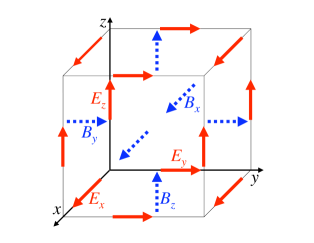
Figure 1: (Color online.) Field components in one grid cell of the Yee mesh. If the above cell has the 3-integer index $(i,j,k)$, then the labeled field components have the same index, e.g., $E_{ijkx}$. The $\mathbf{D}$ components are collocated with the corresponding $\mathbf{E}$ components.

We want to simulate the dynamic Maxwell equations with dielectric:

$$\frac{\partial\bf B}{\partial t} = -\nabla\times{\bf E}$$ (1)

$$\frac{\partial\bf D}{\partial t} = \nabla\times{\bf B}$$ (2)

$$\mathbf{E} = \underline{\underline{\xi}}(x,y,z)\mathbf{D}$$ (3)

where $\underline{\underline{\xi}}=\underline{\underline{\varepsilon}}^{-1}$ is the inverse dielectric tensor (which can vary in space).

To discretize Maxwell’s equations for computational work, we follow Yee [2]. To analyze the discretization, we treat the fields as large vectors, with each component representing a field at one point of the Yee mesh, shown in Fig. 1. (Discretization in time is irrelevant to this paper, so we retain continuous time derivatives.)

For convenience, we label each component of a field vector with 4 sub-indices: e.g., the component $E_{ijkx}$ represents the electric field in the $x$ direction at its Yee location in cell $(i,j,k)$. The differential operators become matrices, with rows and columns each indexed by 4 sub-indices: e.g., one element of a matrix $M$ is $M_{(ijk\mu),(i^{\prime}j^{\prime}k^{\prime}\nu)}$.

We will not review the Yee discretization, since [5] details the relevant aspects, instead taking it for granted that the matrices $C$ and $C^{T}$ represent the curl operators (the matrix representation of the curl of $E$ is the transpose of the curl of $B$). We depart from Yee when we introduce the matrix $\Xi$ to discretize the linear relationship between $E$ and $D$, yielding:

$$\frac{\partial}{\partial t}B_{ijk\mu} = -[CE]_{ijk\mu}$$ (4)

$$\frac{\partial}{\partial t}D_{ijk\mu} = [C^{T}B]_{ijk\mu}$$ (5)

$$E_{ijk\mu} = [\Xi D]_{ijk\mu}=\sum_{i^{\prime}j^{\prime}k^{\prime}\nu}\Xi_{(ijk\mu),(i^{\prime}j^{\prime}k^{\prime}\nu)}D_{i^{\prime}j^{\prime}k^{\prime}\nu}.$$ (6)

These equations are a prescription for advancing the fields in time: $B$ is advanced by a short time (using $E$), then $D$ is advanced (using $B$), then $E=\Xi D$, and the cycle repeats (in practice, this can be implemented with only two fields, $E$ and $B$). Combining these into one equation

$$\frac{\partial^{2}}{\partial t^{2}}B_{ijk\mu} = -[C\Xi C^{T}B]_{ijk\mu}$$ (7)

shows that the eigenvalues $\omega^{2}$ (frequencies squared) of the $-\partial^{2}/\partial t^{2}$ operator are the eigenvalues of the $C\Xi C^{T}$ matrix.

Simulating dielectrics therefore reduces to the determination of $\Xi$ such that

1. $\Xi$ accurately represents the inverse dielectric tensor, $\xi(x,y,z)$, and

2. $C\Xi C^{T}$ is diagonalizable with only real, non-negative eigenvalues.

The first point addresses accuracy. The second addresses robustness/stability: if $C\Xi C^{T}$ has negative or complex eigenvalues, some frequencies $\omega$ will be complex, and some fields will grow exponentially (unphysically), ultimately overwhelming the simulation with noise.

If $\Xi$ is symmetric and positive definite (SPD), then the second point above will be guaranteed: all modes will oscillate (with real frequency) without growing (cf., [5], or a standard linear algebra text such as [9])—at least for a sufficiently small time step. (As stated, temporal discretization is outside the focus of this paper).

This paper is devoted to finding an SPD matrix $\Xi$ that accurately represents dielectric media.

4 Creating a stable $\Xi$ matrix from local $\xi$ tensors

Our approach to dielectric simulation falls under the “effective dielectric” category, specifying the matrix $\Xi$ to find $E=\Xi D$, while advancing $D$ (and $B$) in time according to the unaltered Yee algorithm [2].

As in Ref. [6], we demand that $\Xi$ have the following properties.

1. In case of uniform (anisotropic) dielectric, $\Xi$ involves only centered interpolations of fields (i.e., interpolations with $O(\Delta x^{2})$ error for continuous fields).

2. Within uniform, isotropic dielectric, $\Xi$ reduces to a multiple of the identity.

3. $\Xi$ must be symmetric.

4. $\Xi$ must be positive definite.

The first property yields a local $O(\Delta x^{2})$ error within uniform dielectric (or even continuously-varying dielectric [5]). The second is for convenience and minimalism—we can still use the plain Yee algorithm for fields within any bulk isotropic region. Together, the third and fourth properties guarantee stability. (For comparison: wc07 satisfies 1, 2, and 3.)

Before defining the $\Xi$ matrix, we need to introduce notation for an effective dielectric tensor involving field components of a single Yee cell. For example, we consider the “triplet” of three $E_{\mu}$ values labeled in Fig. 1 and the three $D_{\mu}$ values at the same locations, along edges that touch a common node (corner) of the cell. If the node index is $(ijk)$, then this triplet comprises $(E_{ijkx},E_{ijky},E_{ijkz})$, and similarly $(D_{ijkx},D_{ijky},D_{ijkz})$. (We call these components a triplet, instead of a 3-vector, because they are not collocated.) The triplets for $E$ and $D$ can be related by a $3\times 3$ tensor, $\xi_{ijk}^{+++}$:

$$\mathbf{E}_{ijk}=\xi_{ijk}^{+++}\mathbf{D}_{ijk}\quad\textrm{or}\quad E_{ijk\mu}=\sum_{\nu=x,y,z}\xi_{ijk,\mu\nu}^{+++}D_{ijk\nu}$$ (8)

(the meaning of the $+\!+\!+$ superscript will be explained shortly). Defined thus, $\xi_{ijk}^{+++}$ is an effective (inverse) dielectric tensor for this particular triplet of $E$ and $D$ values.

Touching the same cell node are seven other (eight, in all) geometrically-identical triplets. Above, we chose a triplet with edges extending positively in each direction from their common node, but (due to the symmetries of the Yee mesh) we could equally well have chosen, e.g., the $x$-edge extending in the negative $x$ direction, namely $(E_{(i-1)jkx},E_{ijky},E_{ijkz})$, and $(D_{(i-1)jkx},D_{ijky},D_{ijkz})$. With this triplet, we associate a different effective dielectric, $\xi_{ijk}^{-++}$, with the minus sign indicating that the $E_{x}$ and $D_{x}$ edges extend in the negative $x$ direction from node $(ijk)$.

We will construct (the large matrix) $\Xi$ from the (small) $\xi_{ijk}^{\pm\pm\pm}$ tensors, through an intermediate stage involving (large, block-diagonal matrices) $\Xi^{\pm\pm\pm}$. Symmetry and positive definiteness transfer easily from one stage to the next: we will show that $\Xi$ is SPD if all the $\xi_{ijk}^{\pm\pm\pm}$ are SPD; since the latter are mere $3\times 3$ matrices, evaluating their positive definiteness is easy, numerically if not analytically.

We start by creating block-diagonal matrices $\Xi^{+++}$, $\Xi^{-++}$, …, $\Xi^{---}$, where the blocks are the $\xi_{ijk}^{\pm\pm\pm}$; for example, each block of $\Xi^{-++}$ is $\xi_{ijk}^{-++}$ for some node $(ijk)$. Precisely we define

$$\begin{array}[]{r@{\;}c@{\;}l}\Xi^{+++}_{(ijk\mu)(i^{\prime}j^{\prime}k^{\prime}\nu)}&\equiv&\delta_{(ijk)(i^{\prime}j^{\prime}k^{\prime})}\xi_{ijk,\mu\nu}^{+++}\\ \Xi^{++-}_{(ijk\mu)(i^{\prime}j^{\prime}k^{\prime}\nu)}&\equiv&\xi^{++-}_{ij,k+\delta_{\mu z},\mu\nu}\delta_{(ij,k+\delta_{\mu z}),(i^{\prime}j^{\prime},k^{\prime}+\delta_{\nu z})}\\ \Xi^{+-+}_{(ijk\mu)(i^{\prime}j^{\prime}k^{\prime}\nu)}&\equiv&\xi^{+-+}_{i,j+\delta_{\mu y},k,\mu\nu}\delta_{(ij+\delta_{\mu y},k),(i^{\prime}j^{\prime}+\delta_{\nu y},k^{\prime})}\\ \Xi^{+--}_{(ijk\mu)(i^{\prime}j^{\prime}k^{\prime}\nu)}&\equiv&\xi^{+--}_{i,j+\delta_{\mu y},k+\delta_{\mu z},\mu\nu}\delta_{(ij+\delta_{\mu y},k+\delta_{\mu z}),(i^{\prime}j^{\prime}+\delta_{\nu y},k^{\prime}+\delta_{\nu z})}\\ &\vdots&\\ \Xi^{---}_{(ijk\mu)(i^{\prime}j^{\prime}k^{\prime}\nu)}&\equiv&\xi^{---}_{i+\delta_{\mu x},j+\delta_{\mu y},k+\delta_{\mu z},\mu\nu}\delta_{(i+\delta_{\mu x},j+\delta_{\mu y},k+\delta_{\mu z}),(i^{\prime}+\delta_{\nu x},j^{\prime}+\delta_{\nu y},k^{\prime}+\delta_{\mu z})}\\ \end{array}$$ (9)

where $\delta_{(ijk)(i^{\prime}j^{\prime}k^{\prime})}$ is the Kronecker delta, equal to one when $i=i^{\prime}$, $j=j^{\prime}$, and $k=k^{\prime}$, and otherwise equal to zero. A block-diagonal matrix is SPD if and only if each block is SPD; therefore, if each $\xi_{ijk}^{+++}$ is SPD, then $\Xi^{+++}$ is SPD, and likewise for all $\Xi^{\pm\pm\pm}$.

We finish by taking the $\Xi$ matrix to be the average,

$$\Xi\equiv\frac{1}{8}\left(\Xi^{+++}+\Xi^{++-}+\Xi^{+-+}+\Xi^{-++}+\Xi^{+--}+\Xi^{-+-}+\Xi^{--+}+\Xi^{---}\right).$$ (10)

Since the sum of SPD matrices is again SPD, $\Xi$ is SPD. Figure 2 illustrates how this scheme determines $E_{ijkx}$ from neighboring $D$ values.

Thus we can create a stable algorithm independent of the details of the $\xi_{ijk}^{\pm\pm\pm}$, which can be chosen to improve accuracy at the dielectric interface, within broad constraints: the $\xi_{ijk}^{\pm\pm\pm}$ must be SPD. In addition, when node $(ijk)$ is within uniform dielectric and far from a dielectric interface, $\xi_{ijk}^{\pm\pm\pm}$ must equal $\xi(x,y,z)$, where $(x,y,z)$ is the position of node $(i,j,k)$. This guarantees that, within isotropic dielectric, each $\Xi_{\pm\pm\pm}$ is a multiple of the identity, and so $\Xi$ satisfies requirement 2, above. Furthermore, within uniform dielectric, the algorithm becomes identical to wc07 (see Fig. 3), which uses centered interpolation to yield $O(\Delta x^{2})$ error (within uniform dielectric [5]). Therefore, $\Xi$ satisfies requirements 1 and 2 (as well as 3 and 4).

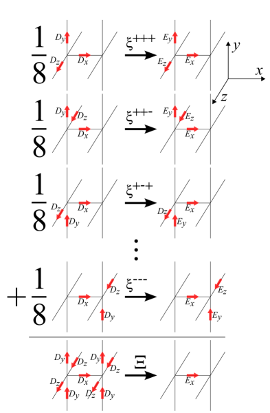
Figure 2: (Color online.) A pictorial representation $E=\Xi D$, showing how $E_{x}$ in cell $(i,j,k)$ is found from neighboring components of $D$. For each of 8 “triplets” a local effective inverse dielectric $\xi$ (a $3\times 3$ matrix) converts $D$ to $E$. Ultimately $E_{x}$ is found using 8 different $\xi$ matrices, one for each triplet involving $E_{x}$. By averaging over all 8 triplets, $E_{x}$ depends symmetrically on its neighboring $D_{y}$ and $D_{z}$, which yields a centered algorithm that, in uniform (or continuously-varying) dielectric, has second-order error [5]. We note that 4 of the triplets use $\xi^{+\pm\pm}_{ijk}$ and 4 use $\xi^{-\pm\pm}_{(i+1)jk}$.

It is easy to forget, when viewing the algorithm as a way to find a single $E_{x}$ (as in Fig. 2), that $\xi^{+-+}_{ijk,xx}$, $\xi^{+-+}_{ijk,xy}$, and $\xi^{+-+}_{ijk,xz}$ must come from the same (SPD) tensor $\xi^{+-+}_{ijk}$. Indeed, it was forgetting which $\xi_{ijk,\mu\nu}$ had to be mathematically related to each other that led to the instability of wc07.

To reiterate: each $\Xi^{\pm\pm\pm}$ matrix is block-diagonal, with $3\times 3$ blocks ($\xi^{\pm\pm\pm}_{ijk}$), each of which represents the effective dielectric tensor around node $(ijk)$. As long as the $\xi_{ijk}^{\pm\pm\pm}$ are SPD, the $\Xi^{\pm\pm\pm}$ are SPD. This further implies that the average, Eq. 10, is SPD.

We have thus shown how to find a stable matrix $\Xi$, given the ability to find $3\times 3$ effective inverse dielectric tensors that map a triplet of neighboring components $(D_{x},D_{y},D_{z})$ to the $(E_{x},E_{y},E_{z})$ at the same locations. Moreover, within uniform (isotropic or anisotropic) dielectric, this algorithm is identical to wc07 (hence it satisfies requirements 1 and 2).

It remains to find the effective dielectric tensors $\xi^{\pm\pm\pm}_{ijk}$ that will accurately represent the real dielectric. Reference [6] showed how to find $\xi^{\pm\pm\pm}_{ijk}$ with local $O(\Delta x)$ error, yielding global $O(\Delta x^{2})$ error; unfortunately, those $\xi^{\pm\pm\pm}_{ijk}$ are asymmetric.

In the next section, we will describe the effective dielectric tensors that yield the wc07 algorithm; some of those tensors may not be positive definite, so that algorithm can be unstable. We then describe a modification to make it stable. However, another effective dielectric turns out to yield lower error (Sec. 7). We have tried several other effective dielectrics, and found them less accurate, but always yielding ultimate $O(\Delta x)$ global error (even stairstepped dielectrics have $O(\Delta x)$ error).

5 The wc07 method, unstable at high contrast

Experiment tells us that wc07 (the algorithm of [5]) can be unstable; therefore, we need concern ourselves no more with that algorithm. However, it is interesting to see exactly how these algorithms differ, so in this section we describe wc07 within the framework of this paper, and show why it does not meet the previously-described (sufficient, but not necessary) conditions for a stable algorithm.

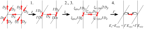
Figure 3: (Color online.) A pictorial representation of $E=\Xi D$ as suggested in [5]. $E_{x}$ in cell $(i,j,k)$ is found from $D_{x}$ at the same location and the nearest $D_{y}$ and $D_{z}$ values. The $I^{\pm}$ are interpolation operators (see [5]).

Figure 3 depicts the wc07 method recommended in [5] [where it is called (c)$+$(e)]. To find $E_{x}$ from its nearest-neighbor $D_{\mu}$ values:

1. perform a centered interpolation of $D_{y}$ and $D_{z}$ to the nearest cell node;

2. find $E_{x(x)}=\xi^{(e)}_{xx}D_{x}$, using the effective dielectric $\xi^{(xe)}$ at the $x$-edge center;

3. find $E_{x(y)}=\xi^{(n)}_{xy}D_{y}$ at each node, using the effective dielectric $\xi^{(n)}$ at that node; similarly, find $E_{x(z)}=\xi^{(n)}_{xz}D_{z}$ at each node;

4. interpolate the two $E_{x(y)}$ from each node to the center of the $x$-edge where $E_{x}$ and $D_{x}$ are located; interpolate $E_{x(z)}$ similarly.

Finally, $E_{x}$ is the sum of parts coming from $E_{x(x)}$, $E_{x(y)}$, and $E_{x(z)}$.

In the framework of the previous section, wc07 is a choice of effective $\xi^{\pm\pm\pm}$:

$$\xi^{\pm\pm\pm}_{ijk,\mu\nu}=\xi^{\pm\pm\pm}_{ijk,\nu\mu} = \xi^{(n)}_{ijk,\mu\nu}\quad(\textrm{for\ }\mu\neq\nu)$$

$$\xi^{+\pm\pm}_{ijk,xx}=\xi^{-\pm\pm}_{(i+1)jk,xx} = \xi^{(xe)}_{ijk,xx}$$ (11)

$$\xi^{\pm+\pm}_{ijk,yy}=\xi^{\pm-\pm}_{i(j+1)k,yy} = \xi^{(ye)}_{ijk,yy}$$

$$\xi^{\pm+\pm}_{ijk,zz}=\xi^{\pm\pm-}_{ij(k+1),yy} = \xi^{(ze)}_{ijk,zz}$$

The tensors $\xi^{(n)}_{ijk}$, $\xi^{(xe)}_{ijk}$, $\xi^{(ye)}_{ijk}$, and $\xi^{(ze)}_{ijk}$ are all to be found from the averaging method of [1], where $\xi^{(n)}_{ijk}$ is the “average” of $\xi(x,y,z)$ over a cell volume centered at the node (lowest corner) of cell $(i,j,k)$, and $\xi^{(xe)}_{ijk}$ is the “average” over a cell volume centered at the location of $E_{ijkx}$ (the $x$-edge-center), etc.

These $\xi_{ijk}^{\pm\pm\pm}$ do not satisfy the conditions for the effective dielectric required by the previous section. E.g., $\xi^{+++}_{ijk}$ is symmetric, but it is not necessarily positive definite. The reason is that the diagonal and off-diagonal elements of $\xi^{+++}_{ijk}$ come from different tensors: $\xi^{(n)}_{ijk}$, $\xi^{(xe)}_{ijk}$, $\xi^{(ye)}_{ijk}$, and $\xi^{(ze)}_{ijk}$. Each of these four tensors is SPD (using the averaging method of [1], cf. B), but there’s no guarantee that a tensor with a mixture of elements from those tensors is positive definite.

Indeed, we have found experimentally that the wc07 algorithm can yield an instability when the dielectric contrast is high enough. We hasten to point out that we have used that algorithm successfully on a wide range of problems without noticing any instability. An instability seems to be more likely for higher contrast, and for larger and more complicated dielectric shapes.

By using the Gershgorin circle theorem to place a lower bound on the eigenvalues of the $\Xi$ matrix (if the lower eigenvalue bound is positive, then $\Xi$ is positive definite, assuming $\Xi$ is symmetric), we can prove for many particular simulations that the algorithm is in fact stable. For example, we usually find that simulations with $\epsilon\leq 10$ are provably stable (on an individual basis, by examining $\Xi$ with the Gershgorin circle theorem).

Many simulations appear stable for long times even when not provably stable. Of course, it’s hard to know whether there might be unstably-growing modes that would dominate the simulation if run 100 times longer; and such unstable modes might interfere with precision measurements well before they become obviously apparent.

For a 2D simulation of photonic crystal modes of a square lattice of isotropic dielectric discs in vacuum (radius $r=0.37a$, where $a$ is the lattice constant), we have seen that at $\epsilon=60$ we can run simulations with $48^{2}$ cells for a time 3000$a/c$ (where $c$ is the speed of light) without seeing an instability (which rules out instabilities growing faster than $\gamma\sim 0.01c/a$, which corresponds to growth of 16 orders of magnitude in 3000$a/c$). For $64^{2}$ cells, however, an instability grows as $\exp(\gamma t)$, where $\gamma\approx 0.5c/a$.

For the same problem, with contrast $\epsilon=100$, it’s harder to find stability for any resolution. For $32^{2}$ cells, an instability grows with $\gamma\approx 3c/a$, and for $64^{2}$ cells, $\gamma\approx 6c/a$.

6 wc07mod: a small change yields stability

In this section we make a small change to the wc07 algorithm that renders it stable. Although this algorithm, which we will call “wc07mod,” is not the most accurate, we present it because it is a relatively trivial modification of wc07, and the resulting degradation of accuracy is interesting, in light of the small modification, which still uses the same averaging method to find the effective dielectric within a given cell-sized volume.

In the language of this paper, this algorithm is described simply as

$$\xi^{\pm\pm\pm}_{ijk\mu\nu}=\xi^{\pm\pm\pm}_{ijk\nu\mu} = \xi^{(n)}_{ijk,\mu\nu}$$ (12)

where $\xi^{(n)}_{ijk}$ is the “average” inverse dielectric tensor for a cell volume centered at the node of cell $(i,j,k)$—where averaging is done according to [1].

Only the diagonal elements of the effective dielectric change, compared to Eq. (5).

In the language of [5], we need simply replace, e.g., in Eq. (27e) of [5] or in step 2 of the wc07 algorithm:

$$\xi^{(xe)}_{ijkxx}\quad \rightarrow \quad\frac{1}{2}\left[\xi^{(n)}_{ijkxx}+\xi^{(n)}_{(i+1)jkxx}\right]$$ (13)

and similarly for the $yy$ and $zz$ elements.

7 The new method

The most accurate local effective dielectric, from [6], yields local $O(\Delta x)$ error, but is unfortunately asymmetric (except for a few surface cuts: e.g., when a planar surface is parallel to a grid plane). Simply symmetrizing it increases the error to $O(1)$, but turns out to be more accurate than other (symmetric) effective dielectrics.

Section 4 reduced the problem of finding a stable $\Xi$ matrix to the problem of finding SPD $3\times 3$ matrices, e.g., $\xi^{+-+}_{ijk}$, that map a triplet of neighboring components $(D_{x},D_{y},D_{z})$ to the $(E_{x},E_{y},E_{z})$ at the same locations—in a way that accurately represents the real dielectric. In this section, we describe the best such recipe that we have found.

While we focus on finding the effective dielectric for a single triplet, we will omit the $(+\!-\!+)$ and $(ijk)$ super- and sub-scripts, which identify the triplet.

This effective dielectric, which is not a volume-averaged dielectric as in [8, 1], derives from Ref. [6], which finds the unique $3\times 3$ tensor $\xi_{\rm acc}$ that guarantees that $(E_{x},E_{y},E_{z})^{T}=\xi_{\rm acc}(D_{x},D_{y},D_{z})^{T}$ will be exactly accurate in the limit of infinite wavelength and planar interface. In other words, $\xi_{\rm acc}$ will convert $(D_{x},D_{y},D_{z})$ to $(E_{x},E_{y},E_{z})$ with no error, given that the triplets are from the finite-difference (or rather, finite integration) representation of an infinite-wavelength solution of Maxwell’s equations. Unfortunately, as we have mentioned, $\xi_{\rm acc}$ is not symmetric.

To achieve stability in the time-domain, we will use

$$\xi_{\rm eff}=\frac{1}{2}\left(\xi_{\rm acc}+\xi_{\rm acc}^{T}\right).$$ (14)

This will be stable; its accuracy will be evaluated empirically.

Finding $\xi_{\rm acc}$ is a lengthy process fully described in [6], so we present only a terse recipe for converting a triplet $(D_{x},D_{y},D_{z})$ to $(E_{x},E_{y},E_{z})$ in the presence of two dielectric regions, $\epsilon_{1}$ and $\epsilon_{2}$ (both symmetric tensors).

1. Within a small region around the triplet (we use the cell volume centered at the nearest node), the dielectric interface is nearly planar; find the unit surface normal $\hat{\bf n}$.

2. Each electric field component $E_{\mu}$ is associated with a cell edge $L_{\mu}$; for each edge, determine the fraction $\ell_{\mu}$ of its length in dielectric $\epsilon_{1}$. See [6] for explicit definition of $L_{\mu}$ (and $A_{\mu}$ in the following).

3. Each component $D_{\mu}$ is associated with a dual-face area $A_{\mu}$ (centered at the Yee location of $D_{\mu}$, perpendicular to $\mu$); for each area, determine the fraction $a_{\mu}$ of the area in $\epsilon_{1}$.

4. Form the $3\times 3$ matrices (for $p=1,2$)

   $$\Gamma_{p} \equiv I+\frac{1}{\hat{\bf n}^{T}\epsilon_{p}\hat{\bf n}}[\hat{\bf n}\hat{\bf n}^{T}](I-\epsilon_{p})$$ (15)

   $$\Pi_{p} \equiv \epsilon_{p}\Gamma_{p}$$ (16)

   $$\Gamma \equiv \left(\begin{array}[]{ccc}\ell_{x}&0&0\\ 0&\ell_{y}&0\\ 0&0&\ell_{z}\\ \end{array}\right)\Gamma_{1}+\left(\begin{array}[]{ccc}1-\ell_{x}&0&0\\ 0&1-\ell_{y}&0\\ 0&0&1-\ell_{z}\\ \end{array}\right)\Gamma_{2}$$ (23)

   $$\Pi \equiv \left(\begin{array}[]{ccc}a_{x}&0&0\\ 0&a_{y}&0\\ 0&0&a_{z}\\ \end{array}\right)\Pi_{1}+\left(\begin{array}[]{ccc}1-a_{x}&0&0\\ 0&1-a_{y}&0\\ 0&0&1-a_{z}\\ \end{array}\right)\Pi_{2}$$ (30)

   where $[\hat{\bf n}\hat{\bf n}^{T}]$ is the dyadic matrix with elements $[\hat{\bf n}\hat{\bf n}^{T}]_{\mu\nu}=\hat{n}_{\mu}\hat{n}_{\nu}$, and $I$ is the identity.

5. The accurate effective (inverse) dielectric tensor is:

   $$\xi_{\rm acc} = \Gamma\Pi^{-1}$$ (31)

   We then symmetrize that to find

   $$\xi_{\rm eff} = \frac{1}{2}(\xi_{\rm acc}+\xi_{\rm acc}^{T})$$ (32)

6. The above can fail if $\Pi$ is not invertible, and if the resulting $\xi_{\rm eff}$ is not positive definite. Failure is ruled out for isotropic dielectrics [6], and for anisotropic dielectrics, it has not yet happened in our experience. Nevertheless, it’s important to guard against pathological cases. We suggest checking every $\xi_{\rm eff}$ for these two problems; if one should occur, then substitute the effective dielectric from [1] (which is proven suitable in B). This will happen so rarely, if ever, that the global error will not be significantly affected.

8 Simulation Results

We tested various FDTD algorithms on different dielectric problems: a square lattice of 2D isotropic and anisotropic dielectric discs in vacuum; a square lattice of 2D vacuum discs (holes) in isotropic dielectric; and a cubic lattice of 3D dielectric spheres in vacuum, for both isotropic and anisotropic dielectric. For many of these cases, we also tested different dielectric contrasts. We define $a$ to be the lattice constant, and $N_{a}$ the number of (square or cubic) cells per lattice constant, hence $\Delta x=a/N_{a}$.

Ultimately, the FDTD algorithms all show first-order error in frequency; the error in a mode frequency falls as $O(\Delta x)$, or $O(\Delta x/\lambda)$, where $\lambda$ is a characteristic wavelength of the mode, with decreasing cell size $\Delta x$. However, at coarse resolutions (large $\Delta x$), the error often falls as $O(\Delta x^{2})$ for low dielectric contrast. This may explain why previous studies have concluded that methods such as wc07 have second-order error—they did not explore high-enough resolution or contrast (of course, in practice, one may often reach a tolerable error level within the second-order regime, in which case the ultimate order of error may be irrelevant).

The error convergence in surface fields was the same as in frequencies when we considered the surface fields a fixed distance (e.g., $a/8$) away from the dielectric boundary. However, the error in fields a fixed number of cells (e.g., $3\Delta x$) away from the boundary, is $O(1)$, not $O(\Delta x)$. This supports our assertion that the local error at the boundary, due to discontinuous fields, is $O(1)$, but the global error is $O(\Delta x)$ because the ratio of boundary cells to total cells is $O(\Delta x)$.

We performed the FDTD simulations with Vorpal [4] using the FDM method [10] to extract accurate mode fields and frequencies. We compared these results with the frequency-domain algorithm of [6], which was shown to have second-order global error. For 2D simulation frequencies, we extrapolated results from $N_{a}=512$ and $N_{a}=1024$ assuming second-order convergence to get a normative value with approximately $O(\Delta x^{3})$ error.

We will show the most detailed convergence results for the “new” algorithm (Sec. 7) for 2D anisotropic discs. Isotropic and 3D dielectrics show similar convergence, so we present only a few examples.

We will show that the other FDTD algorithms, wc07 and wc07mod generally have similar or greater error compared to the new algorithm; and the other examples (3D and isotropic) show qualitatively similar convergence.

For comparison, we also show frequency convergence for the second-order (but unstable in the time-domain) method of [6] in A.

8.1 Convergence: 2D anisotropic discs

We simulated TE modes (with $E_{z}=0$, $B_{x}=0=B_{y}$, and no variation in $z$) in a square lattice (lattice constant $a$) of dielectric discs of radius $r=0.37a$ in vacuum; the discs were of dielectric

$$\epsilon = \epsilon_{b}\left(\begin{array}[]{ccc}1.025&-\sqrt{3}/40&0\\ -\sqrt{3}/40&1.075&0\\ 0&0&1.\\ \end{array}\right)$$ (36)

where we vary the scalar $\epsilon_{b}$ to vary the dielectric contrast. For $\epsilon_{b}=10$, the above is the diagonal matrix $(10,11,10)$ rotated by 30 degrees around the $z$-axis.

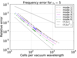
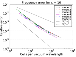
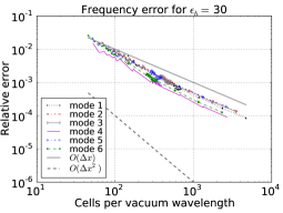
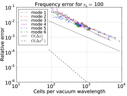
Figure 4: (Color online.) For the new algorithm presented in this paper, relative errors vs. resolution for mode frequencies for a 2D photonic crystal of $r/a=0.37$ anisotropic discs with varying dielectric contrast $\epsilon_{b}$. The error transitions from second-order to first-order at higher resolutions. The transition point occurs at coarser resolution for higher dielectric contrast.

Figure 4 shows the relative error in the frequency of the lowest several modes vs. the number of cells per vacuum wavelength (or $c$ divided by the mode frequency), for dielectric contrast of $\epsilon_{b}=5,10,30,100$. Low contrast simulations, $\epsilon_{b}\lesssim 10$, yield second-order error to rather high resolutions. At sufficiently high resolution, the error becomes first-order; this is more clearly seen in the mid-contrasts. For high contrast, $\epsilon_{b}\gtrsim 30$, the second-order region is too small to notice, and first-order convergence is clear.

There is a problem in examining the convergence of the fields. The fields are discontinuous at the dielectric interface, and it is not obvious how best to interpolate the fields near the interface. There is a danger, when choosing an interpolation method, that it might not be the best interpolation method. Therefore, we avoid the interface. Staying at least $3\Delta x$ (where $\Delta x$ is the cell size) away from the surface, there is no serious ambiguity in interpolation: a simple bilinear (or, in 3D, trilinear) interpolation should be sufficient for errors of at least $O(\Delta x^{2})$.

We examine field-convergence in two ways.

First, we generate a set of (evenly-distributed) points on a circle at a radius $a/8$ larger than the interface, and, at each resolution, interpolate the mode fields to those points, comparing against our normative values (from the algorithm of [6]) using the $\ell_{2}$-norm over the set of points (after normalizing the entire eigenmodes). We then graph the relative error vs. resolution. We find (not surprisingly) that it converges at the same rate (ultimately $O(\Delta x)$) as the mode frequencies (Fig. 5).

For $\epsilon_{b}=100$, modes 4 and 5 have relatively large errors in the surface field; qualitatively, however, the modes look more accurate than the $\ell_{2}$ norm suggests. These modes place most of the field energy inside the dielectric; they resemble a pair of quadrupole (e.g., $\textrm{TE}_{21}$) modes in a circular waveguide: that is, the field patterns have nearly (but not exactly, due to the square lattice) an azimuthal dependence $\cos(2\theta+\theta_{0})$ and $\cos(2\theta+\theta_{0}+\pi/2)$ for some angle $\theta_{0}$. If the dielectric were isotropic, these modes would be degenerate, and $\theta_{0}$ could be chosen arbitrarily (since there is a linear combination of the above two terms that yields $\cos(2\theta+\theta_{0}^{\prime})$ for any $\theta_{0}^{\prime}$). With the anisotropic dielectric, the mode frequencies differ by about 0.3%, and so $\theta_{0}$ is determined. It appears that the error is so high because the eigenmodes have a large error in $\theta_{0}$. In other words, the field patterns look very similar to the correct fields, except they are rotated slightly. This is a consequence of the difficulty of eigensolving for nearly-degenerate modes; as two modes approach degeneracy it becomes impossible to separate them correctly (without recourse to some other operator). In this light, it is not surprising that when the error in frequency is larger than the actual separation between the two modes, the resulting eigenmodes may be the wrong linear combinations of the exact eigenmodes. Indeed the surface error starts diminishing for modes 4 and 5 approximately when the frequency errors approach 0.3% (see Fig. 4).

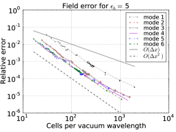
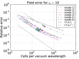
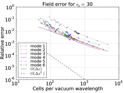
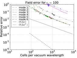
Figure 5: (Color online.) For the new method, 2D, anisotropic: relative error (in an $\ell_{2}$-norm) vs. resolution in $\mathbf{E}$ at points on a circle of radius $a/8$ outside the dielectric interface, for a 2D photonic crystal of anisotropic discs with varying dielectric contrast $\epsilon_{b}$. At high resolutions, the error is first-order.

Second, we generate a set of points on a circle that is a radius $3\Delta x$ outside the interface; thus each different resolution has a different set of points; as simulation resolution increases, the points move closer to the actual interface. For each resolution, the fields are compared to our normative high-resolution simulation. In this case, the error does not vanish with $\Delta x$; in other words, it is $O(1)$ (Fig. 6).

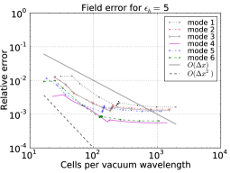
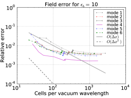
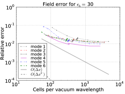
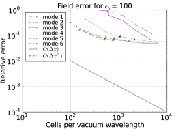
Figure 6: (Color online.) For the new method, 2D, anisotropic: relative error (in an $\ell_{2}$-norm) vs. resolution in $\mathbf{E}$ at points on a sphere of radius $(0.37+3\Delta x)a$ for a 2D photonic crystal of anisotropic discs with varying dielectric contrast $\epsilon_{b}$. This error does not go to zero as $\Delta x\rightarrow 0$.

This latter conclusion is disquieting for those who want particularly to measure fields at the interface. However, we point at that the error, although $O(1)$, can be quite low, especially for low dielectric contrast. For dielectric contrast $\leq 15$, the relative error in field is less than one percent. The error drops significantly as one moves away from the interface, and we believe it might be possible to extrapolate the fields from several cells away to find surface fields with vanishing error as $\Delta x\rightarrow 0$.

The wc07 method [5, 7], and indeed all the effective FDTD dielectric methods we’ve tried, have very similar error convergence, transitioning from second- to first-order at a resolution that decreases as the dielectric contrast increases. We believe this may explain a discrepancy that has puzzled us: this work and [5] see first-order error (in mode frequencies) for this effective dielectric, while the results of [7] show second-order error. The latter uses two anisotropic dielectrics, one with eigenvalues (1.45, 2.81, 4.98), and another with (8.49, 8.78, 11.52), both rotated by random orthogonal matrices. At contrast $11.52/1.45\approx 8$, we do in fact see second-order behavior up to hundreds of cells per wavelength, and for contrasts between other pairs (e.g., $8.49/4.98$), second-order behavior persists up to higher resolutions than we have explored.

In fact, practically, it must be said that the effective dielectric in [1, 7] does yield second-order behavior for low-contrast dielectric up to nearly the highest resolutions that one might practically use. Ultimately, however, it has first-order error.

For low contrasts, the local error associated with the dielectric interface doesn’t see to have much effect, and so the results are similar for different algorithms.

8.2 Convergence: 2D isotropic discs

To show that using isotropic dielectric (instead of anisotropic) does not change the order of error, we present frequency convergence results for the same problem in the previous section, except that the dielectric is replaced with an isotropic dielectric $\epsilon=\epsilon_{b}$. Figure 7 shows frequency error convergence for $\epsilon_{b}=15$ and $\epsilon_{b}=100$. The former shows a gradual transition from second-order to first-order error, while the the higher contrast shows just first-order error.

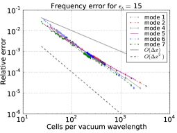
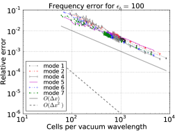
Figure 7: (Color online.) For the new method, 2D, isotropic: relative errors vs. resolution for mode frequencies for a 2D photonic crystal of $r/a=0.37$ isotropic discs with dielectric contrast $\epsilon_{b}=15$ (left) and $\epsilon_{b}=100$ (right). Again, the error transitions from second-order to first-order. The transition point occurs at coarser resolution for higher dielectric contrast.

8.3 Convergence: 3D isotropic spheres

Figure 8 shows frequency convergence for a 3D cubic lattice of isotropic spheres ($r/a=0.37$) with $\epsilon=15$ and $\epsilon=30$. Although the computational requirements prevent exploration over the wide range of resolutions of the 2D simulations, the $\epsilon=15$ case shows mostly second-order behavior starting to transition to first-order, while $\epsilon=30$ shows nearly first-order behavior. This is very similar to Fig. 4, considering the resolutions where they overlap. There is no reason to suspect that error convergence in 3D is any different from 2D.

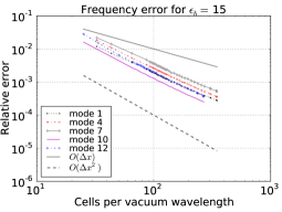
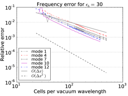
Figure 8: (Color online.) For the new method, 3D, isotropic: relative errors vs. resolution for mode frequencies for a 3D cubic lattice of spheres with isotropic $\epsilon=15$ (left) and $\epsilon=30$ (right), using the algorithm of Sec. 7. For $\epsilon=15$ convergence is second-order for low resolution, but gradually moves toward first-order; for $\epsilon=30$, convergence is nearly first-order.

8.4 Comparison to wc07: 2D and 3D, aniso- and iso-tropic

In this section we compare the “new” method recommended in this paper (Sec. 7) to wc07 (which uses the effective dielectric of [8]), except we improved wc07 for anisotropic dielectrics by using the effective dielectric of [1, 7].

The main advantage of the new method is that it is always stable; since wc07 is usually stable for contrasts less than $\epsilon=30$, and can be used practically, we wanted to compare their accuracies. The new method is generally better than wc07, by a small factor (2–10), for higher contrasts and resolutions. We cannot compare them for contrasts at $\epsilon=100$ because the old method becomes unstable.

For low contrast, and low resolution, there is less reason to choose one algorithm over the other—for some modes one is better, for other modes the other is better. However, even for $\epsilon=5$, the new method can yield more accurate fields, even while the frequencies are more or less equally accurate. Of course, there may be geometries and contrasts for which wc07 is better.

Figure 9 shows the error for wc07 divided by the error for the new method, for the 2D square lattice of anisotropic discs (as in Sec. 8.1). Not only is the new method guaranteed stable, it performs better for medium and high dielectric contrast.

Occasionally, for a problem of low contrast, one sees the error of wc07 plunge at some low resolution; the same sometimes happens for other methods as well. In this case, it appears that the frequency error has first- and second-order contributions: $\alpha\Delta x+\beta\Delta x^{2}$. When $\alpha$ and $\beta$ have opposite signs, there is a narrow range of $\Delta x$ for which the error is nearly zero. However, this drop in frequency error is not reflected in the field error. An example of this can be seen for $\epsilon=5$ in Figs. 13 and 14.

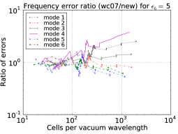
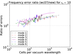
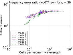
Figure 9: (Color online.) For wc07/new, 2D, anisotropic: the frequency error in wc07 over the error in the new algorithm, for modes of a 2D photonic crystal of $r/a=0.37$ anisotropic discs with dielectric contrast $\epsilon_{b}$. For $\epsilon_{b}\gtrsim 10$, the new method has lower frequency error; however, Fig. 10 shows that even for $\epsilon_{b}=5$, the new method has lower field error.

Figure 10 shows the error of algorithm wc07 divided by that of the new algorithm for surface fields on the circle at $r/a=0.37+1/8$. In nearly all cases, the wc07 algorithm has higher error. The error ratio is seen to increase with the number of cells per vacuum wavelength.

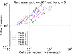
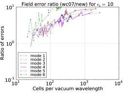
Figure 10: (Color online.) For wc07/new, 2D, anisotropic: the field error in wc07 over the error in the new algorithm, for fields on a circle at $r/a=0.37+1/8$, a fixed distance outside the dielectric disc. The new method is better in almost every case, even for $\epsilon_{b}=5$. (The simulations are the same as in Fig. 9.)

A similar advantage for the new method is also apparent in 3D, as shown in Fig. 11, for sapphire (anisotropic, $\epsilon_{b}\approx 10$) and isotropic, $\epsilon_{b}=15$ spheres. The dielectric tensor for the sapphire spheres was

$$\epsilon = \left(\begin{array}[]{ccc}10.225&-0.825&-0.55\sqrt{3/2}\\ -0.825&10.225&0.55\sqrt{3/2}\\ -0.55\sqrt{3/2}&0.55\sqrt{3/2}&9.95\\ \end{array}\right)$$ (40)

which has $\epsilon=11.6$ along its $c$-axis, and $9.4$ in the two perpendicular directions; we took the $c$-axis along $y$, and then rotated the dielectric by $30^{\circ}$ about the $x$-axis, and then $45^{\circ}$ about the $z$-axis.

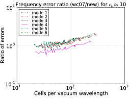
Figure 11: (Color online.) For wc07/new, 3D, aniso- and iso-tropic: the frequency error in wc07 over the error in the new algorithm, for modes of a 3D photonic crystal of $r/a=0.37$ spheres of sapphire (left) and isotropic $\epsilon=15$ (right).

The advantage of the new method remains when the concavity of the dielectric interface changes: Figure 12 shows the advantage of the new method for vacuum discs in a background of $\epsilon_{b}$.

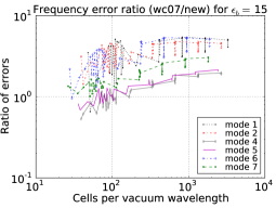
Figure 12: (Color online.) For wc07/new, 2D, isotropic (inverse): the frequency error in wc07 over the error in the new algorithm, for modes of a 2D photonic crystal of $r/a=0.37$ vacuum discs (holes) inside an isotropic background of $\epsilon=15$.

8.5 Comparison to wc07mod: 2D anisotropic discs

Here we compare the new algorithm to the wc07mod algorithm (Sec. 6), for the modes of a square lattice of $r/a=0.37$ anisotropic discs, as before. The new algorithm is better except (surprisingly, given how much worse wc07mod is at medium contrast) for $\epsilon_{b}=100$.

Figure 13 shows the ratio in frequency errors. For low contrast, we see that the error for wc07mod plunges within a narrow range of resolutions, due to fortuitous cancellation of first- and second-order error; we note that one cannot depend on this cancellation (it does not occur for all shapes, nor is the range of resolutions predictable). This is illustrated by the convergence of field, where such fortuitous cancellation is much less likely; there, wc07mod has no less error.

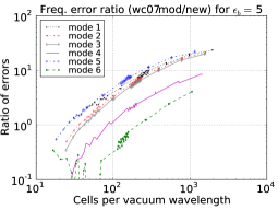
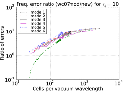
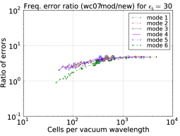
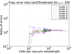
Figure 13: (Color online.) For wc07mod/new, 2D, anisotropic: the frequency error in wc07mod over the error in the new algorithm, modes of a 2D photonic crystal of $r/a=0.37$ anisotropic discs with dielectric contrast $\epsilon_{b}$.

Figure 14 shows the ratio of the surface field error of the wc07mod algorithm to that of the new algorithm on a circle at $r/a=0.37+1/8$. This shows that the wc07mod algorithm generally has higher error, and that the factor by which it is worse increases with the number of cells per vacuum wavelength.

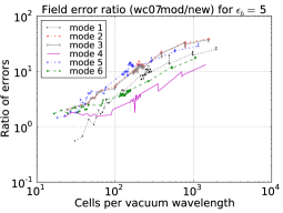
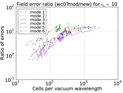
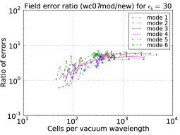
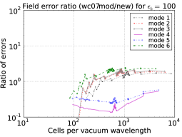
Figure 14: (Color online.) For wc07mod/new, 2D, anisotropic: the field error in wc07mod over the error in the new algorithm, for fields on a circle at $r/a=0.37+1/8$, a fixed distance outside the dielectric disc.

9 Summary and Discussion

We have demonstrated a new FDTD algorithm for simulating electromagnetics in the presence of sharp dielectric transitions; the new algorithm is generally as accurate or more accurate than previous FDTD algorithms, and it is stable at high dielectric contrast (unlike the algorithm of [5, 7]).

We showed how to create a stable algorithm, given the ability to form an “effective” (or “average”) $3\times 3$ dielectric tensor relating any three neighboring components of the $D$-field and the $E$-field. As long as each $3\times 3$ tensor is symmetric and positive definite (SPD), the algorithm will be stable. One can then try to construct SPD effective dielectric tensors to achieve the highest accuracy.

We compared three different ways to compute the effective dielectric: a sometimes unstable method, wc07, described in [5, 7]; a small alteration of that method to achieve stability, wc07mod, but still using the dielectric averaging of [1]; and a new method based on symmetrizing the asymmetric effective dielectric of [6].

All these algorithms (except [6], which is unstable in the time domain) have first-order error in the grid-cell-size $\Delta x$; that is, the error in mode frequencies and fields at given points decreases ultimately as $O(\Delta x)$. However, at coarse resolutions the error decreases as $O(\Delta x^{2})$, before transitioning to $O(\Delta x)$. For low dielectric contrast (less than about 10), the transition point occurs at fairly high resolution, so that for many simulations, these methods may be practically considered to have second-order error.

By examining the convergence of mode fields, we showed that the fields at fixed points (fixed as $\Delta x$ varies) converge at the same rate as the mode frequencies. However, when we look at the fields at a fixed cell-distance away from a dielectric interface (so that the points move closer to the interface as $\Delta x$ decreases), we find that the error is $O(1)$—it does not decrease with $\Delta x$.

This demonstrates two important points. First, the global error is $O(\Delta x)$: the local error in the bulk material is $O(\Delta x^{2})$ (due to centered differencing), is (eventually) eclipsed by the $O(1)$ local error at the interface (due to the discontinuity in fields). However, the interface cuts a fraction of cells scaling as $O(\Delta x)$, so the ultimate global error (e.g., in mode frequency) in $O(\Delta x)$. Heuristically, we can write “$\textrm{Error}=a\Delta x+b\Delta x^{2}$,” where $a$ comes from the interface, and $b$ from the bulk (as well higher order terms from the interface). Our results show that $a$ can be relatively small for low dielectric contrast, and therefore the error at low resolutions (large $\Delta x$) appears second-order for a while. Sometimes $a$ and $b$ may be of opposite signs, in which case the error may plunge briefly for a small range of $\Delta x$ at the transition between second- and first-order (but only for frequency error; field error is not a one-dimensional quantity like frequency, and so the first- and second-order parts cannot fortuitously cancel).

Although we cannot prove that the symmetric effective dielectrics used in FDTD simulations must yield (ultimate) first-order error, the logic of [6] strongly hints that should be the case. Reference [6] achieved second-order error by demanding local first-order, or $O(\Delta x)$, error at the dielectric interface—accomplished by finding an effective dielectric that exactly maps $\mathbf{D}$ to $\mathbf{E}$ in the limit of infinite wavelength (and planar interface). Unfortunately, that effective dielectric is asymmetric, and unusable in FDTD codes due to the instability it creates. Equally unfortunate, the symmetric effective dielectrics do not appear to be able to satisfy this property of mapping $\mathbf{D}$ to $\mathbf{E}$ exactly in the infinite wavelength limit.

The $O(1)$ convergence of error at a fixed cell-distance from the surface could be a problem for finding surface fields with arbitrary accuracy. However, the error drops rapidly by several cells away from the surface, and we believe that it will be possible to obtain surface fields with arbitrary accuracy by extrapolating from the fields several cells away from the surface. Of course, that extrapolation introduces some error, but we currently believe that the field error plus the extrapolation error can be made to vanish as $\Delta x\rightarrow 0$. However, a much more thorough study will be needed in the future to determine this issue.

It would be great if we could somehow form a symmetric effective dielectric with the accuracy of the asymmetric effective dielectric of [6]. Indeed, there are some degrees of freedom one could exploit. For example, we used a symmetric average of the $\Xi^{\pm\pm\pm}$ matrices is Sec. 4 to form $\Xi$. We could have have used different non-negative coefficients (not $1/8$) that add up to one, without affecting stability; however, the accuracy within uniform, anisotropic dielectric would be degraded. In principle, one can vary those coefficients in space; however, varying them can destroy the symmetry of $\Xi$, so one would need some sort of global solution to attain accuracy and symmetry (not to mention positive definiteness). We have made some attempts to do this, without complete success. There may be a way; if not, it may still be possible to achieve greater accuracy, though not as high as [6], while maintaining stability.

10 Acknowledgments

This work was supported by the U.S. Department of Energy grant DE-FG02-04ER41317.

Most of the simulations described in this work were performed with the Vorpal framework; we would like to acknowledge the efforts of the Vorpal team: D. Alexander, K. Amyx, E. Angle, T. Austin, G. I. Bell, D. L. Bruhwiler, E. Cormier-Michel, Y. Choi, B. M. Cowan, R. K. Crockett D. A. Dimitrov, M. Durant, B. Jamroz, M. Koch, S. E. Kruger, A. Likhanskii, M. C. Lin, M. Loh, J. Loverich, S. Mahalingam, P. J. Mullowney, C. Nieter, K. Paul, I. Pogorelov, C. Roark, B. T. Schwartz, S. W. Sides, D. N. Smithe, P. H. Stoltz, S. A. Veitzer, D. J. Wade-Stein, N. Xiang, C. D. Zhou.

Appendix A The error in the asymmetric second-order method

To demonstrate what second-order convergence looks like, we show convergence using the results for the 2D anisotropic dielectric problem for $\epsilon_{b}=10$ and $\epsilon_{b}=100$ using the algorithm of [6] in Fig. 15. Here we compare to the Richardson-extrapolated values from simulations at resolutions $N_{a}=512$ and $N_{a}=1024$ (and therefore, we do not plot the values for $N_{a}=1024$).

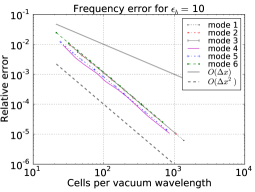
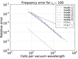
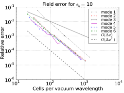
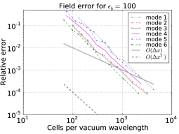
Frequency Error Field Error ($a/8$ outside interface) Field Error ($3\Delta x$ outside interface)

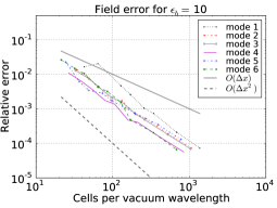
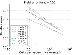
Figure 15: (Color online.) For the second-order method, 2D, anisotropic: relative error vs. resolution for the second-order method of [6] (which would be unstable in the time-domain), for the anisotropic 2D photonic crystal with $\epsilon_{b}=10$ (left) and $\epsilon_{b}=100$ (right). Errors shown are in frequency (top), and in $\mathbf{E}$ (middle) for a circle at radius $(0.37+1/8)a$, and (bottom) for a circle of radius $(0.37+3\Delta x)a$. As expected, global errors (top and middle) are $O(\Delta x^{2})$, but local field errors at the interface are ultimately $O(\Delta x)$ (as clearly seen in $\epsilon_{b}=100$).

The code used to produce these graphs is open-sourced at https://github.com/bauerca/maxwell.

Appendix B The effective dielectric tensor of (Kottke, 2008) is positive semi-definite

If two dielectrics, $\varepsilon^{1}$ and $\varepsilon^{2}$, coexist in a cell in which the normal to the interface between dielectrics is $\hat{\bf n}$, then we compute the effective dielectric as follows, according to [1].

Rotating into a coordinate system where the first coordinate is $\hat{\bf n}$ (the other two directions, perpendicular to $\hat{\bf n}$, are labeled 2 and 3), we calculate $\tau^{1}$ and $\tau^{2}$:

$$\tau^{i}\equiv\tau(\varepsilon^{i})\equiv\left(\begin{array}[]{c@{\quad}c@{\quad}c}\displaystyle-\frac{1}{\varepsilon^{i}_{nn}}&\displaystyle\frac{\varepsilon^{i}_{n2}}{\varepsilon^{i}_{nn}}&\displaystyle\frac{\varepsilon^{i}_{n3}}{\varepsilon^{i}_{nn}}\\ \displaystyle\frac{\varepsilon^{i}_{2n}}{\varepsilon^{i}_{nn}}&\displaystyle\varepsilon^{i}_{22}-\frac{\varepsilon^{i}_{2n}\varepsilon^{i}_{n2}}{\varepsilon^{i}_{nn}}&\displaystyle\varepsilon^{i}_{23}-\frac{\varepsilon^{i}_{2n}\varepsilon^{i}_{n3}}{\varepsilon^{i}_{nn}}\phantom{\frac{{|^{|}}^{|}}{{|_{|}}_{|}}}\\ \displaystyle\frac{\varepsilon^{i}_{3n}}{\varepsilon^{i}_{nn}}&\displaystyle\varepsilon^{i}_{32}-\frac{\varepsilon^{i}_{3n}\varepsilon^{i}_{n2}}{\varepsilon^{i}_{nn}}&\displaystyle\varepsilon^{i}_{33}-\frac{\varepsilon^{i}_{3n}\varepsilon^{i}_{n3}}{\varepsilon^{i}_{nn}}\\ \end{array}\right).$$ (41)

According to [1], $\tau$ (not, e.g., $\epsilon$) is the quantity that should be volume-averaged. We perform a simple average on $\tau^{1}$ and $\tau^{2}$ to get the effective $\tilde{\tau}$, and then transform back to get the effective $\tilde{\varepsilon}$.

$$\varepsilon(\tau)=\left(\begin{array}[]{c@{\quad}c@{\quad}c}\displaystyle-\frac{1}{\tau_{nn}}&\displaystyle-\frac{\tau_{n2}}{\tau_{nn}}&\displaystyle-\frac{\tau_{n3}}{\tau_{nn}}\\ \displaystyle-\frac{\tau_{2n}}{\tau_{nn}}&\displaystyle\tau_{22}-\frac{\tau_{2n}\tau_{n2}}{\tau_{nn}}&\displaystyle\tau_{23}-\frac{\tau_{2n}\tau_{n3}}{\tau_{nn}}\phantom{\frac{{|^{|}}^{|}}{{|_{|}}_{|}}}\\ \displaystyle-\frac{\tau_{3n}}{\tau_{nn}}&\displaystyle\tau_{32}-\frac{\tau_{3n}\tau_{n2}}{\tau_{nn}}&\displaystyle\tau_{33}-\frac{\tau_{3n}\tau_{n3}}{\tau_{nn}}\\ \end{array}\right).$$ (42)

For example, if the volume fractions for $\varepsilon^{1}$ and $\varepsilon^{2}$ are $V_{1}$ and $V_{2}$, respectively ($V_{1}+V_{2}=1$), then the effective dielectric is

$$\tilde{\varepsilon}=\varepsilon(V_{1}\tau^{1}+V_{2}\tau^{2}).$$ (43)

We can show that, if $\varepsilon^{1}$ and $\varepsilon^{2}$ are symmetric and positive semi-definite (SPSD), then $\tilde{\varepsilon}$ is also SPSD.

We remember that a real, symmetric matrix $A$ is positive semi-definite when, for all $x$, $x^{T}Ax\geq 0$. It follows that the sum of SPSD matrices is again SPSD.

Whenever $A$ is real and SPSD, there exists a matrix $P$ such that $A=P^{T}P$. The reverse also holds: if $A=P^{T}P$, then for all $x$, $x^{T}Ax=x^{T}P^{T}Px=\|Px\|^{2}\geq 0$. From this we can conclude that $Q^{T}AQ=(PQ)^{T}(PQ)$ is SPSD for any matrix $Q$.

We will prove that $\tilde{\varepsilon}=\varepsilon(\tilde{\tau})=\varepsilon(V_{1}\tau^{1}+V_{2}\tau^{2})$ is SPSD, by showing that there is an invertible matrix $\Gamma$ such that $\Gamma^{T}\tilde{\varepsilon}\Gamma$ is SPSD.

The matrix $\Gamma$

$$\Gamma(\varepsilon)=\left(\begin{array}[]{c@{\quad}c@{\quad}c}\displaystyle\frac{1}{\varepsilon_{nn}}&\displaystyle-\frac{\varepsilon_{n2}}{\varepsilon_{nn}}&\displaystyle-\frac{\varepsilon_{n3}}{\varepsilon_{nn}}\\ \displaystyle 0&1&0\\ 0&0&1\\ \end{array}\right)$$ (44)

is invertible, since it is diagonalizable and none of its eigenvalues ($1/\epsilon_{nn}$, $1$, and $1$) are zero. The matrix product

$$\Gamma^{T}\varepsilon\Gamma=\left(\begin{array}[]{c@{\quad}c@{\quad}c}\displaystyle\frac{1}{\varepsilon_{nn}}&0&0\\ 0&\displaystyle\varepsilon_{22}-\frac{\varepsilon_{2n}\varepsilon_{n2}}{\varepsilon_{nn}}&\displaystyle\varepsilon_{23}-\frac{\varepsilon_{2n}\varepsilon_{n3}}{\varepsilon_{nn}}\phantom{\frac{{|^{|}}^{|}}{{|_{|}}_{|}}}\\ 0&\displaystyle\varepsilon_{32}-\frac{\varepsilon_{3n}\varepsilon_{n2}}{\varepsilon_{nn}}&\displaystyle\varepsilon_{33}-\frac{\varepsilon_{3n}\varepsilon_{n3}}{\varepsilon_{nn}}\\ \end{array}\right)=\left(\begin{array}[]{c@{\quad}c@{\quad}c}\displaystyle-\tau_{nn}&0&0\\ 0&\displaystyle\tau_{22}&\displaystyle\tau_{23}\\ 0&\displaystyle\tau_{32}&\displaystyle\tau_{33}\\ \end{array}\right)$$ (45)

is SPSD whenever $\varepsilon$ is (since $x^{T}\Gamma^{T}\varepsilon\Gamma x=(\Gamma x)^{T}\varepsilon(\Gamma x)$). Since $\Gamma$ is invertible the converse also holds: if $\Gamma^{T}\varepsilon\Gamma$ is positive semi-definite, then so is $\varepsilon$.

All this means that because the $\varepsilon^{i}$ are SPSD, $\Gamma(\varepsilon^{i})^{T}\varepsilon^{i}\Gamma(\varepsilon^{i})$ are SPSD. Since $\tilde{\tau}=V_{1}\tau^{1}+V_{2}\tau^{2}$, the matrix

$$\Gamma(\tilde{\varepsilon})^{T}\tilde{\varepsilon}\Gamma(\tilde{\varepsilon}) = \left(\begin{array}[]{c@{\quad}c@{\quad}c}\displaystyle-\tilde{\tau}_{nn}&0&0\\ 0&\displaystyle\tilde{\tau}_{22}&\displaystyle\tilde{\tau}_{23}\\ 0&\displaystyle\tilde{\tau}_{32}&\displaystyle\tilde{\tau}_{33}\\ \end{array}\right)=V_{1}\Gamma(\varepsilon^{1})^{T}\varepsilon^{1}\Gamma(\varepsilon^{1})+V_{2}\Gamma(\varepsilon^{2})^{T}\varepsilon^{2}\Gamma(\varepsilon^{2})$$ (49)

is the sum of two positive semi-definite matrices, which is itself positive semi-definite. Therefore the effective dielectric tensor, $\tilde{\varepsilon}$ is positive semi-definite.

Incidentally, the matrix $\Gamma$ plays a well-known role. If $\mathbf{F}=(D_{n},E_{2},E_{3})$ is the 3-tuple of continuous field components (at the dielectric interface), then $\mathbf{F}=\Gamma(\varepsilon)\mathbf{E}$. In fact, the effective dielectric is derived (see [1]) by taking the perturbative formula for change in eigenvalue:

$$\Delta\omega^{2}\propto\langle E|\varepsilon(x)-\varepsilon^{\prime}(x)|E^{\prime}\rangle$$ (51)

where $E$ is the eigenmode corresponding to $\varepsilon(x)$ and $E^{\prime}$ is the (exact) eigenmode corresponding to $\varepsilon^{\prime}(x)$. The above expression contains no approximation; the problem is that one typically doesn’t know $E^{\prime}$—usually a first-order approximation is realized by approximating $E^{\prime}\approx E$. In this case, the authors of [1] argued that because $E$ is discontinuous, it jumps when $\varepsilon$ changes by a finite amount, and so $E^{\prime}\approx E$ is a bad approximation (it has zeroth-order error). It is better to approximate $F^{\prime}\approx F$. Therefore, we write

$$\Delta\omega^{2} \propto \langle E|\varepsilon(x)-\varepsilon^{\prime}(x)|E^{\prime}\rangle=\langle F|\Gamma(\varepsilon)^{T}[\varepsilon(x)-\varepsilon^{\prime}(x)]\Gamma(\varepsilon^{\prime})|F^{\prime}\rangle$$ (52)

$$\approx \langle F|\Gamma(\varepsilon)^{T}[\varepsilon(x)-\varepsilon^{\prime}(x)]\Gamma(\varepsilon^{\prime})|F\rangle.$$

To obtain approximately zero frequency shift when we substitute $\epsilon^{\prime}$ for $\epsilon$, we demand that $\int_{V}\Gamma(\varepsilon)^{T}[\varepsilon(x)-\varepsilon^{\prime}(x)]\Gamma(\varepsilon^{\prime})$ vanish, which leads directly to the condition that $\int_{V}\tau(\epsilon(x))=\int_{V}\tau(\epsilon^{\prime}(x))$.

References

- [1] C. Kottke, A. Farjadpour, S. G. Johnson, Perturbation theory for anisotropic dielectric interfaces and application to subpixel smoothing of discretized numerical methods, Phys. Rev. E. 77 (2008) 036611.
- [2] K. S. Yee, Numerical solution of initial boundary value problems involving Maxwell’s equations in isotropic media, IEEE Trans. Antennas Propag. 14 (3) (1966) 302.
- [3] B. Gustafsson, The convergence rate for difference approximations to mixed initial boundary value problems, Math. Comput. 29 (130) (1975) 396.
- [4] C. Nieter, J. R. Cary, VORPAL: a versatile plasma simulation code, J. Comput. Phys. 196 (2) (2004) 448.
- [5] G. R. Werner, J. R. Cary, A stable FDTD algorithm for non-diagonal, anisotropic dielectrics, J. Comput. Phys. 226 (1) (2007) 1085.
- [6] C. A. Bauer, G. R. Werner, J. R. Cary, A second-order 3D electromagnetic algorithm for curved interfaces between anisotropic dielectrics on a Yee mesh, J. Comput. Phys. 230 (5) (2011) 2060.
- [7] A. F. Oskooi, C. Kottke, S. G. Johnson, Accurate finite-difference time-domain simulation of anisotropic media by subpixel smoothing, Opt. Lett. 34 (18) (2009) 2778.
- [8] S. G. Johnson, J. D. Joannopoulos, Block-iterative frequency-domain methods for Maxwell’s equations in a planewave basis, Opt. Express 8 (2001) 173.
- [9] M. Artin, Algebra, Prentice Hall, Inc., 1991.
- [10] G. R. Werner, J. R. Cary, Extracting degenerate modes and frequencies from time-domain simulations with filter-diagonalization, J. Comput. Phys. 227 (10) (2008) 5200.