Abstract

We show that closed string solutions in the bulk of ${AdS}$ space are related by T-duality to solutions representing an open string ending at the boundary of ${AdS}$. By combining the limit in which a closed string becomes small with a large boost, we find that the near-flat space short string in the bulk maps to a periodic open string world surface ending on a wavy line at the boundary. This open string solution was previously found by Mikhailov and corresponds to a time-like near BPS Wilson loop differing by small fluctuations from a straight line. A simple relation is found between the shape of the Wilson loop and the shape of the closed string at the moment when it crosses the horizon of the Poincare patch. As a result, the energy and spin of the closed string are encoded in properties of the Wilson loop. This suggests that closed string amplitudes with one of the closed strings falling into the Poincare horizon should be dual to gauge theory correlators involving local operators and a Wilson loop of the T-dual (“momentum”) theory.

1 Introduction

There are many known relations between closed and open strings. For example, in flat space a world sheet representing a propagation of a closed string may be viewed, after $\tau\leftrightarrow\sigma$ interchange, as describing also propagation of an open string in periodic time; an open string disc diagram for open strings may be viewed as a closed string emission by a D-brane into vacuum; KLT relations express closed string scattering amplitudes in terms of open string scattering amplitudes, etc.

In the gauge-string duality context, one recent example is the relation between the coefficient of the leading logarithmic term in the large spin (long string) asymptotics of the closed folded spinning string energy [1] and the cusp anomalous dimension of the Wilson loop defined by a light-like cusp [2, 3, 4]. There is also a (KLT-like) relation between a correlator of closed string vertex operators at null separations and a square of a Wilson loop defined by the corresponding null polygon [5].

These are cases of far-from-BPS configurations, but there are other examples that hint towards a possible closed-open string relation also for “short” strings or “small” deviations from the BPS limit. According to [6], for a straight line Wilson loop with a small cusp of angle $\pi-\phi$, $\phi\ll 1$ in $AdS_{5}$ one finds

$$\langle W_{\rm cusp}\rangle=\exp\Big{[}-\Gamma_{\rm cusp}(\phi,\lambda)\ln{\Lambda}+...\Big{]}\ ,$$ (1.1)

$$\Gamma_{\rm cusp}(\phi,\lambda)_{{}_{\phi\to 0}}=-B(\lambda)\,\phi^{2}+...\ ,\$$ (1.2)

$$B(\lambda)={\sqrt{\lambda}\over 4\pi^{2}}{I_{2}(\sqrt{\lambda})\over I_{1}(\sqrt{\lambda})}={1\over 4\pi^{2}}\Big{(}\sqrt{\lambda}-{3\over 2}+{3\over 8\sqrt{\lambda}}+...\Big{)}\ .$$ (1.3)

In (1.3) we gave the expansion of the coefficient $B(\lambda)$ at strong coupling or for large string tension, i.e. $\lambda\gg 1$. The same expression is found for a cusp of angle $\pi-\theta$ in $S^{5}$ (with $\phi^{2}\to-\theta^{2}$). It was observed in [8] that switching on an orbital momentum $J$ in $S^{5}$, the expression for the leading $\lambda\gg 1$ term in the corresponding $\Gamma_{\rm cusp}(\theta,\lambda;J)$ appears to be related to the small-spin limit of the energy of a folded spinning string in $S^{3}$.

Moreover, there is a striking similarity [6] between the small angle coefficient $B$ in (1.2) and the slope function [9] found in the small spin limit of the $AdS_{5}$ folded string energy. According to [9, 10, 11], the dimension of the sl(2) sector gauge-theory operator with spin ${\rm S}$ and twist $J$ or the energy of the corresponding dual spinning string state has the following expansion in the formal $S\ll 1$ limit

$$E^{2}=J^{2}+h(\lambda,J)\,{\rm S}+O({\rm S}^{2})\ ,$$ (1.4)

$$h=2J+\bar{h}(\lambda,J)\ ,\ \ \ \ \ \ \ \ \ \bar{h}(\sqrt{\lambda},J)=2\sqrt{\lambda}\,{I_{J+1}(\sqrt{\lambda})\over I_{J}(\sqrt{\lambda})}\ .$$ (1.5)

If one formally sets here $J=1$ then the slope function in (1.5) becomes directly related to $B$ in eq.(1.3), i.e.

$$h(\lambda,1)=2+8\pi^{2}B(\lambda)=2\sqrt{\lambda}-{1}+O({1\over\sqrt{\lambda}})\ .$$ (1.6)

A motivation behind the present work is to try to find a possible relation between small (nearly point-like) closed strings in $AdS_{5}$ and long open strings ending at the boundary (and thus corresponding to nearly-straight Wilson lines).

Let us recall that the coefficient $B(\lambda)$ in (1.2),(1.3) has also other interpretations. As was argued in [6], for a euclidean Wilson loop defined by a curve which is a small transverse deviation from a straight line [14, 15] one has

$$\langle W_{\rm wavy}\rangle=1+{{\textstyle{1\over 2}}}B(\lambda)\int d\sigma d\sigma^{\prime}\ \frac{\left[\partial_{\sigma}\vec{x}_{\perp}(\sigma)-\partial_{\sigma}\vec{x}_{\perp}(\sigma^{\prime})\right]^{2}}{(\sigma-\sigma^{\prime})^{2}}+...\ ,$$ (1.7)

where it is assumed that $|\partial_{\sigma}\vec{x}_{\perp}|\ll 1$. Furthermore, the same $B(\lambda)$ appears also in the expression for the energy emitted [16] by a slowly moving “quark” [6] (see also [13])

$$E=2\pi B(\lambda)\int d\tau\ {\dot{v}}^{2}+...\ ,\ \ \ \ \ \ \ \ \ \ \ \ \vec{v}=\dot{\vec{\rm x}}(\tau)\ \ll 1\ ,$$ (1.8)

where $\vec{x}(\tau)$ is a spatial deviation of the quark’s trajectory from a straight line. As was shown in [16], the Minkowski open-string world surface ending on the quark’s trajectory at the boundary of the Poincare patch leads to the following expression for the classical ($\sqrt{\lambda}\gg 1$) string energy

$$E_{0}={\sqrt{\lambda}\over 2\pi}\int d\tau\ {\dot{v}^{2}-[\vec{v}\times\dot{\vec{v}}]^{2}\over(1-v^{2})^{3}}\approx{\sqrt{\lambda}\over 2\pi}\int d\tau\ \dot{v}^{2}+...\ ,$$ (1.9)

which is a relativistic generalization of the integral in (1.8).

The derivation of the classical energy formula (1.9) is straightforward in the limit of small deviations from a straight line [16]. Using the Poincare patch coordinates $ds^{2}={1\over z^{2}}(dz^{2}-dx_{0}^{2}+dx_{i}^{2})$ and choosing the static gauge

$$x_{0}=\tau,\ \ \ \ \ \ \ \ \ \ \ z=\sigma\ ,$$ (1.10)

the string (Nambu) action for small fluctuations in $x_{i}$-directions is

$$S={\sqrt{\lambda}\over 2\pi}\int{d\tau d\sigma\over\sigma^{2}}\Big{[}1+{1\over 2}(\dot{x}_{i}^{2}-x_{i}^{\prime 2})+O(\partial x^{3})\Big{]}\ .$$ (1.11)

The corresponding equation of motion $\ddot{x}_{i}-x^{\prime\prime}_{i}+2\sigma^{-1}x^{\prime}_{i}=0$ has solution $x_{i}(\tau,\sigma)$ which is uniquely determined by the two boundary data functions – ${\rm x}^{+}(\tau)$ and ${\rm x}^{-}(\tau)$, or, equivalently, the shape of the boundary curve ${\rm x}_{i}(\tau)\equiv x_{i}(\tau,0)={\rm x}^{+}(\tau)+{\rm x}^{-}(\tau)$ and its 3-rd normal derivative [16]. Explicitly, one finds

$$x_{i}(\tau,\sigma) = {\rm x}_{i}(\tau,\sigma)-\sigma\partial_{\sigma}{\rm x}_{i}(\tau,\sigma)$$ (1.12)

$$= {\rm x}^{+}_{i}(\tau+\sigma)+{\rm x}^{-}_{i}(\tau-\sigma)-\sigma\Big{[}\dot{{\rm x}}^{+}_{i}(\tau+\sigma)-\dot{{\rm x}}^{-}_{i}(\tau-\sigma)\Big{]}+O({\rm x}^{2})\ ,$$

$$x_{i}(\tau,0) \equiv {\rm x}_{i}(\tau)={\rm x}^{+}_{i}(\tau)+{\rm x}^{-}_{i}(\tau)\ ,\ \ \ \ \ \ \ \ \ \partial_{\sigma}^{3}x_{i}(\tau,0)=-2\partial_{\tau}^{3}[{\rm x}^{+}_{i}(\tau)-{\rm x}^{-}_{i}(\tau)]\ ,$$ (1.13)

where ${\rm x}_{i}(\tau,\sigma)={\rm x}^{+}_{i}(\tau+\sigma)+{\rm x}^{-}_{i}(\tau-\sigma)$ is generic flat-space solution (harmonic function). The string energy associated with translations in the $x_{0}=\tau$ direction

$$E_{0}={\sqrt{\lambda}\over 2\pi}\int^{\infty}_{0}{d\sigma\over\sigma^{2}}\Big{[}1+{1\over 2}(\dot{x}_{i}^{2}+x_{i}^{\prime 2})+O(\partial x^{3})\Big{]}\ ,\ \ \ \$$ (1.14)

then leads, after renaming the integration variable $\sigma\to\tau$, to the same expression as in (1.9), i.e. ${\sqrt{\lambda}\over 2\pi}\int d\tau\ {\ddot{\rm x}}_{i}^{2}$.

In this paper we will show that T-duality along the boundary directions of $AdS_{5}$ relates the world sheets of small closed strings in the bulk of ${AdS}$ to the open string surfaces ending on wavy lines representing small-velocity “quark” trajectories at the boundary. Our starting point will be the observation that T-duality along the boundary directions in the Poincare patch of ${AdS}$ space maps a massless geodesic in the bulk of ${AdS}$ into a straight line Wilson loop surface.

As was first observed in [17], the formal T-duality along all $x^{\mu}=(x^{0},x^{i})$ boundary directions maps $AdS\$into $AdS\$space provided it is combined with a simple coordinate transformation – the inversion of the radial direction, $z\to 1/z$ (which effectively interchanges the boundary and the horizon).

This T-duality was used (in Euclidean world sheet case) in [18] to relate (imaginary) world sheet solution that dominate a semiclassical path integral for open-string (gluon) scattering amplitudes to (real) solutions describing the corresponding null polygon Wilson loops in the dual momentum space. Here we will be considering the case of the Minkowski signature in both the target space and the world sheet, so that the T-duality transformations will be mapping real solutions into real solutions.

We shall start in section 2 with a review of the basic definitions and properties of T-duality transformation in ${AdS}$ and discuss some simple examples.

In section 3 we shall describe in detail the map between small closed strings and long open strings ending on a nearly straight line at the boundary of ${AdS}$ and thus corresponding to the wavy line Wilson loops.

In section 4 we shall consider an example of application of the T-duality to a closed string of finite size – folded string with an arbitrary spin. Section 5 will contain some comments on a physical interpretation of the T-duality relation and implications for a process of a small closed string crossing a horizon. Some concluding remarks will be made in section 6.

In Appendix A we shall give our definitions of elliptic functions used in section 4. In Appendix B we shall discuss the application of the T-duality transformation to the small spiky string solution. Appendix C contains a discussion of implementation of T-duality on a cylinder a closed string insertion.

2 Definition of T-duality transformation and some examples

Let us start with describing the basic sets of coordinates in ${AdS}_{5}$ we will be using. The embedding coordinates are defined by

$$ds^{2}_{{}_{AdS_{5}}}=dX_{M}dX^{M}\ ,\ \ \ \ \ \ \ \ \ \ -X_{M}X^{M}=X_{-1}^{2}+X_{0}^{2}-X_{1}^{2}-X_{2}^{2}-X_{3}^{2}-X_{4}^{2}=1\ .$$ (2.1)

It is convenient to introduce also the light-like coordinates

$$X_{\pm}=X_{-1}\pm X_{4}\ ,\ \ \ \ \ \ \ \ \ X_{+}X_{-}-X_{\mu}X^{\mu}=1\ ,\ \ \ \ \ \ \ \ \ \ \ X_{\mu}=(X_{0},X_{i})\ .$$ (2.2)

The global coordinates $(t,\rho,\hat{n}_{r})$ are related to $X_{M}$ by

$$X_{0}+iX_{-1}=\cosh\rho\ e^{it},\ \ \ \ \ \ \ \ \ X_{r}=\sinh\rho\ \hat{n}_{r},\ \ \ \ \ \ r=1,\ldots,4\ ,$$ (2.3)

$$ds^{2}=-\cosh^{2}\rho\ dt^{2}+d\rho^{2}+\sinh^{2}\rho\ d\Omega^{2}_{[3]}\ ,$$ (2.4)

where $\hat{n}_{r}$ is a 4-component unit vector parametrising an $S^{3}$. The Poincare coordinates are defined by

$$Z=\frac{1}{X_{-}}\ ,\ \ \ \ \ \ \ \ \ \ X_{-}=X_{-1}-X_{4}=\cosh\rho\,\sin t-\sinh\rho\,\hat{n}_{4}\ ,$$ (2.5)

$${\cal X}_{0}\equiv{\cal T}=\frac{X_{0}}{X_{-}}=\frac{\cosh\rho\,\cos t}{X_{-}}\ ,\ \ \ \$$ (2.6)

$${\cal X}_{i}=\frac{X_{i}}{X_{-}}=\frac{\sinh\rho\ \hat{n}_{i}}{X_{-}}\ ,\ \ \ \ \ \ \ \ i=1,2,3\ ,$$ (2.7)

$$ds^{2}={1\over Z^{2}}(dZ^{2}+d{\cal X}_{\mu}d{\cal X}^{\mu})\ ,\ \ \ \ \ \ \ \ \ \ \ {\cal X}_{\mu}=({\cal T},{\cal X}_{i}),\ \ \ \ \ \ {\mu=0,1,2,3}.$$ (2.8)

We shall use the conformal gauge in which the classical bosonic string action $S={\sqrt{\lambda}\over 2\pi}{\bar{S}}$, equations of motion and the conformal-gauge constraints written in the embedding coordinates are

$${\bar{S}}={1\over 2}\int d\sigma d\tau\left(\partial_{a}X_{+}\partial^{a}X_{-}-\partial_{a}X_{\mu}\partial^{a}X^{\mu}\right)+{1\over 2}\int d\sigma d\tau\Lambda\left(X_{+}X_{-}-X_{\mu}X^{\mu}-1\right)\ ,$$ (2.9)

$$\partial_{a}\partial^{a}X_{\pm}=\Lambda X_{\pm}\ ,\ \ \ \ \ \ \ \ \ \ \ \ \partial_{a}\partial^{a}X^{\mu}=\Lambda X^{\mu}\ ,$$ (2.10)

$$\Lambda=\partial_{a}X_{+}\partial^{a}X_{-}-\partial_{a}X_{\mu}\partial^{a}X^{\mu}\ ,\ \ \ \ \ \ \ \ \ X_{+}X_{-}-X_{\mu}X^{\mu}=1\ ,$$ (2.11)

$$\partial_{\sigma}X_{+}\partial_{\sigma}X_{-}+\partial_{\tau}X_{+}\partial_{\tau}X_{-}-\partial_{\sigma}X_{\mu}\partial_{\sigma}X^{\mu}-\partial_{\tau}X_{\mu}\partial_{\tau}X^{\mu}=0\ ,$$

$$\partial_{\sigma}X_{+}\partial_{\tau}X_{-}+\partial_{\tau}X_{+}\partial_{\sigma}X_{-}-2\partial_{\sigma}X_{\mu}\partial_{\tau}X^{\mu}=0\ .$$ (2.12)

In what follows we shall map one class of solutions of these equations (small closed strings) into another class of their solutions (open-string Wilson-loop type solutions) using the formal T-duality (2-d scalar-scalar duality) transformation that maps $AdS\$into $AdS\$if combined with the $Z\to 1/Z$ coordinate transformation [17]. For brevity, we shall often refer to this combined transformation simply as T-duality.

Using the Minkowski signature in both the target space and the world sheet the T-duality transformation rule is then $(Z,{\cal X}_{\mu})\to(\tilde{Z},\tilde{\cal X}_{\mu})$ where $\partial_{a}\tilde{\cal X}_{\mu}=\epsilon_{ab}Z^{-2}\partial^{b}{\cal X}_{\mu}$ (with $\epsilon_{\tau\sigma}=-1$), i.e.

$$\partial_{\tau}\tilde{\cal X}_{\mu}=-\frac{1}{Z^{2}}\partial_{\sigma}{\cal X}_{\mu}\ ,\ \ \ \ \ \ \partial_{\sigma}\tilde{\cal X}_{\mu}=-\frac{1}{Z^{2}}\partial_{\tau}{\cal X}_{\mu}\ ,\ \ \ \ \ \ \ \ \ \ \tilde{Z}=\frac{1}{Z}=X_{-}\ .$$ (2.13)

Thus $(\tilde{Z},\tilde{\cal X}_{\mu})$ satisfy the same set of equations (2.11),(2.12) corresponding to the dual ${AdS}_{5}$ metric $ds^{2}={1\over\tilde{Z}^{2}}(d\tilde{Z}^{2}+d\tilde{\cal X}_{\mu}d\tilde{\cal X}^{\mu})$. Note that this T-duality is done along non-compact target space directions that leads to subtleties when, as here, the world sheet theory is defined on a cylinder (see Appendix C).

The T-duality relations in (2.13) may be written also as

$$\partial^{a}\tilde{{\cal X}}_{\mu}=-\epsilon^{ab}\,j_{b,-\mu}\ ,$$ (2.14)

$$j_{a,MN}\equiv X_{M}\partial_{a}X_{N}-X_{N}\partial_{a}X_{M}\ ,\ \ \ \ \ \ \partial^{a}j_{a,MN}=0\ ,$$ (2.15)

where $j_{a,MN}$ is the $SO(4,2)$ Noether current associated to the ${AdS}_{5}$ space symmetry which is conserved on the equations of motion (2.11) with the corresponding charge being

$$J_{MN}=\int d\sigma\ j_{\tau,MN}\ .$$ (2.16)

Thus the particular $SO(4,2)$ angular momentum components $J_{-\mu}$ get the interpretation of the “winding numbers” in the dual $\tilde{\cal X}_{\mu}$ directions,   $\int d\sigma\,\partial_{\sigma}\tilde{\cal X}_{\mu}=J_{-\mu}$.

Let us give some simple examples of T-duality applied to string solutions in $AdS$. In general, T-duality formally relates a classical string solution to another solution and thus maps the corresponding sets of conserved charges. For example, the world line of a point-like string or massless geodesic in ${AdS}$ is T-dual to a straight-line Wilson loop surface (in Minkowski world-sheet signature). In more detail, the T-duality counterparts for the three simple solutions in $\mbox{${AdS}_{2}$}\subset\mbox{${AdS}_{5}$}$ are (after T-duality it is convenient to interchange $\sigma$ and $\tau$):

$\bullet$ massless geodesic in $AdS_{2}$ ($t=t(\tau),\ \rho=\rho(\tau)$,  $\sinh\rho=\kappa\tau,\ \tan t=\kappa\tau,\ \,\cos t={1\over\sqrt{1+\kappa^{2}\tau^{2}}}$)

$$Z={\cal T}={1\over\kappa\tau}\ ,\ \ \ \ \ \ \ \ \ \ \ \ \ \ \ \tilde{Z}=\kappa\sigma\ ,\ \ \ \ \ \ \tilde{\cal T}=\kappa\tau\ .$$ (2.17)

The dual surface reaches the boundary at $\sigma=0$ where it is a straight line along $\tilde{\cal T}\sim\tau$. The reason we interchanges $\sigma$ and $\tau$ after T-duality is precisely to have the new time coordinate $\tilde{\cal T}$ proportional to $\tau$ (instead of $\sigma$).

$\bullet$ massive geodesic ($t=\kappa\tau$, $\rho=0$) or a massless BMN geodesic in $AdS_{2}\times S^{1}$ (with $S^{1}$ angle $\varphi=\kappa\tau$ not involved in the T-duality transformation)

$$Z={1\over\sin\kappa\tau}\ ,\ \ \ \ \ {\cal T}=\cot\kappa\tau\ ,\ \ \ \ \ \ \ \ \ \ \ \ \tilde{Z}=\sin\kappa\sigma\ ,\ \ \ \ \tilde{\cal T}=\kappa\tau\ .$$ (2.18)

The dual surface ends at the boundary at $\sigma=0$ where it is a straight line along $\tilde{\cal T}$ and then again at $\kappa\sigma={\pi\over 2}$. Notice that the dual surface has two boundaries corresponding to the intersection of the initial surface with the past and future Poincare Horizons.

$\bullet$ wrapped string ($t=\kappa\tau$, $\varphi=\kappa\sigma$ where $\varphi$ is an angle of a maximal circle of $S^{5}$)

$$Z={1\over\sin\kappa\tau}\ ,\ \ \ \ \ {\cal T}=\cot\kappa\tau\ ,\ \ \ \ \ \ \ \ \ \ \ \ \tilde{Z}=\sin\kappa\sigma\ ,\ \ \ \ \tilde{\cal T}=\kappa\tau,\ \ \ \ \varphi=\kappa\tau\ .$$ (2.19)

Here we again interchanged $\tau$ and $\sigma$ after T-duality.

$\bullet$ infinite straight static string in $AdS_{2}$ ($t=\kappa\tau,\ \rho=\rho(\sigma)$, $\tanh{\rho\over 2}=\tan{\kappa\sigma\over 2},$ $\cosh\rho={1\over\cos\kappa\sigma}$)

$$Z={\cos\kappa\sigma\over\sin\kappa\tau}\ ,\ \ \ \ \ {\cal T}=\cot\kappa\tau\ ,\ \ \ \ \ \ \ \ \ \ \ \ \ \ \ \ \tilde{Z}={\sin\kappa\sigma\over\cos\kappa\tau}\ ,\ \ \ \ \tilde{\cal T}=\tan\kappa\tau\ .$$ (2.20)

Here the original solution reaches the boundary ($\rho=\infty$) at $\kappa\tau={\pi\over 2}$ where it ends on a line along ${\cal T}$. The dual solution ends at the boundary for $\kappa\sigma={\pi\over 2}n$ on a line along $\tilde{\cal T}$.

It is clear from these examples that to interpret the T-dual world surface as that of an open string stretched inside ${AdS}$ and ending at the boundary at a point (“quark”) one needs to do two steps:

(i) Formally “decompactify” the $\sigma$ direction. Starting with a periodic solution for a small closed string (defined on a 2d cylinder) and applying the T-duality (in a particular gauge, see below) we will get a $\sigma$-periodic open-string world sheet, apart from the $\tilde{\cal T}$ direction which gets a term linear in $\sigma$. As discussed in Appendix C, the world-sheet theory will still be periodic since $\tilde{\cal T}$ enters only through its derivatives (assuming there are no vertex operator insertions depending on $\tilde{\cal T}$).

(ii) Interchange the $\tau$ and $\sigma$ coordinates (a familiar operation in the usual flat-space closed–open string duality relation).

Let us briefly mention another example – the large spin limit of folded spinning string in $AdS_{3}$ ($ds^{2}=-\cosh^{2}\rho\ dt^{2}+d\rho^{2}+\sinh^{2}\rho\ d\theta^{2}$) which is an infinite rotating string stretching all the way to the boundary [22]: $t=\theta=\kappa\tau,\ \ \rho=\kappa\sigma$, $\kappa\to\infty$. This solution is known to be related [3], via a Euclidean world-sheet continuation and an $SO(2,4)$ transformation, to the null cusp Wilson loop solution [2]. The T-duality provides a different relation to an open-string world sheet ending at the boundary. Indeed, absorbing $\kappa$ into $\sigma$ and $\tau$ and thus making their range infinite we get (${\cal X}\equiv{\cal X}_{1}$)

$$Z=(\cosh\sigma\,\sin\tau-\sinh\sigma\,\cos\tau)^{-1},\ \ {\cal T}=Z\cosh\sigma\,\cos\tau,\ \ {\cal X}=Z\sinh\sigma\,\sin\tau\ ,$$ (2.21)

$$\tilde{Z}={\cosh\sigma\,\sin\tau-\sinh\sigma\,\cos\tau}\ ,\ \ \ \tilde{\cal T}={{\textstyle{1\over 2}}}\big{(}-\tau+\sigma-\sin\tau\,\cos\tau+\sinh\sigma\,\cosh\sigma\big{)}\ ,$$ (2.22)

$$\tilde{\cal X}={{\textstyle{1\over 2}}}\big{(}-\tau-\sigma+\sin\tau\,\cos\tau+\sinh\sigma\,\cosh\sigma\big{)}\ ,$$

$$\tilde{\cal T}+\tilde{\cal X}=-\tau+\sinh\sigma\,\cosh\sigma\ ,\ \ \ \ \ \ \tilde{\cal T}-\tilde{\cal X}=\sigma-\sin\tau\,\cos\tau\ .$$ (2.23)

The T-dual surface ends at the boundary $\tilde{Z}=0$ when $\tan\tau=\tanh\sigma$ where

$$\tilde{\cal T}+\tilde{\cal X}=-{\rm arctan}(\tanh\sigma)+{1\over 2}\sinh 2\sigma\ ,\ \ \ \ \ \ \tilde{\cal T}-\tilde{\cal X}=\sigma-{1\over 2}\tanh 2\sigma\ .$$ (2.24)

To have an open-string interpretation we are again to replace $\sigma\leftrightarrow\tau$. The boundary trajectory is a bended curve passing through zero in $(\tilde{\cal T},\tilde{\cal X})$ plane (at large $\tau$ one has $\tilde{\cal T}+\tilde{\cal X}\sim e^{2(\tilde{\cal T}-\tilde{\cal X})}$).

Our aim below will be to apply the above T-duality transformation to small (“short”) strings in the bulk of ${AdS}_{5}$. To study short strings that effectively probe the near-flat limit of ${AdS}_{5}$ it is useful to consider a neighbourhood of linear size $\epsilon\rightarrow 0$ around the point $X_{0}=1$, $X_{M\neq 0}=0$, namely

$$X_{0}\sim 1+\epsilon^{2}\ ,\ \ \ \ \ \ \ \ \ \ \ \ \ X_{M\neq 0}\sim\epsilon\ .$$ (2.25)

An example one may have in mind is a small string of size $\epsilon$ oscillating near $\rho=0$. In this case the components of the Noether current $j_{a,MN}$ in (2.15) scale as

$$j_{a,0M}\sim\partial_{a}X_{M}\sim\epsilon,\ \ \ \ \ j_{a,MN}\sim\epsilon^{2},\ \ \ \ \ \ \ \ \ \mbox{for}\ \ M,N\neq 0\ .$$ (2.26)

In particular, $j_{a,-0}\sim\epsilon$ whereas $j_{a,-i}\sim\epsilon^{2}$.

In addition to this scaling limit, an important ingredient of our discussion will be a particular $SO(4,2)$ transformation – a large boost in the $(X_{+},X_{-})$ hyperbolic plane of the embedding 4-space in (2.1)

$$X_{-}\rightarrow\frac{1}{\epsilon}X_{-},\ \ \ \ \ \ \ \ X_{+}\rightarrow\epsilon X_{+}\ ,\ \ \ \ \ \ \ \ \ \epsilon\rightarrow 0\ .$$ (2.27)

This boost makes a small string near $\rho=0$ move fast towards the boundary, following approximately a massless geodesic. This exposes the near-BPS nature of a nearly point-like small string state.

Assuming that the $\epsilon$ parameters in (2.25) and in (2.27) are the same, the resulting scaling of the components of $j_{a,MN}$ after the boost is

$$j_{a,-0}\sim 1,\ \ \ \ \ \ \ j_{a,-i},\,j_{a,0i}\sim\epsilon,\ \ \ \ \ \ \ j_{a,+-},\,j_{a,ij},\,j_{a,+0}\sim\epsilon^{2},\ \ \ \ \ \ \ j_{a,+i}\sim\epsilon^{3}\ .$$ (2.28)

The components entering the T-duality relation in (2.14) are then

$$j_{a,-0}\simeq\partial_{a}X_{-}\sim 1,\ \ \ \ \ \ \ \ \ \ \ j_{a,-i}=X_{-}\partial_{a}X_{i}-X_{i}\partial_{a}X_{-}\sim\epsilon\ ,$$ (2.29)

implying that for $J_{MN}$ in (3.24) one has $J_{-0}\sim 1$ and $J_{-i}\sim\epsilon$. This means, in the T-dual interpretation, that the dual string is extended along $\tilde{{\cal X}}_{0}=\tilde{{\cal T}}$ with fluctuations of order $\epsilon$ in the directions $\tilde{{\cal X}}_{i=1,2,3}$. Since $X_{-}\sim 1$ the dual string world sheet extends also along $\tilde{Z}=1/Z=X_{-}$.

It is useful to record the scaling of the conserved charges representing the energy and the spin of a short string we started with (we omit the factor of string tension, i.e. $E={\sqrt{\lambda}\over 2\pi}\bar{E}$, etc.)

$$\bar{E} \equiv J_{-0}+J_{+0}=\int\!d\sigma\,\partial_{\tau}X_{-}+{\cal O}(\epsilon^{2})\ ,$$ (2.30)

$$\bar{\rm S}_{ij} \equiv J_{ij}={\cal O}(\epsilon^{2})\ .$$ (2.31)

To summarise, (i) expanding around the point $X_{0}=1$, $X_{M\neq 0}=0$ in ${AdS}_{5}$ and (ii) performing a large boost in the $X_{\pm}$ plane with the same parameter $\epsilon$ as the expansion scale produces a string configuration which has the T-dual interpretation as a world sheet extended along $\tilde{{\cal T}}$, $\tilde{Z}$ with small fluctuations in the spatial $\tilde{{\cal X}}_{i=1,2,3}$ directions. We shall study this relation in detail in the following section.

3 T-duality relation between short closed strings and long wavy open strings

Let us elaborate on the small string expansion discussed above. Starting with global coordinates in (2.4) we may set

$$\rho=\epsilon\bar{\rho},\ \ \ \ \ \ \ \ t=\epsilon y_{0}\ ,$$ (3.1)

so that the metric becomes nearly flat

$$ds^{2} = -\cosh^{2}\rho dt^{2}+d\rho^{2}+\sinh^{2}\rho d\Omega_{[3]}^{2}$$ (3.2)

$$\simeq \epsilon^{2}\left(-dy_{0}^{2}+dy_{r}dy_{r}\right)\ ,\ \ \ \ \ \ \ \ y_{r}=\bar{\rho}\hat{n}_{r}\ ,$$ (3.3)

where $\hat{n}_{r}$ is the unit vector in (2.3).

The corresponding small string equations will be the same as in flat space. Let us fix the conformal gauge and further choose a particular conformal parametrisation (light-cone gauge) where

$$y_{-}\equiv y_{0}-y_{4}=\tau\ .$$ (3.4)

Then the solution for the transverse spatial directions $y_{i}$ is the usual flat-space one

$$y_{i}(\sigma,\tau)={\rm y}_{i}(\sigma,\tau)\equiv{\rm y}_{i}^{+}(\sigma+\tau)+{\rm y}_{i}^{-}(\sigma-\tau)\ ,\ \ \ \ \ \ \ \ \ \ \ i=1,2,3$$ (3.5)

with an initial value at $\tau=0$ given by

$$y_{i}(\sigma,0)={\rm y}_{i}(\sigma)={\rm y}_{i}^{+}(\sigma)+{\rm y}_{i}^{-}(\sigma)\ .$$ (3.6)

As we shall explain below, this leading-order small-string configuration is T-dual to an open-string solution ending at the boundary along the following trajectory (after $\tau\leftrightarrow\sigma$ interchange)

$${\cal X}_{0}=\tau\ ,\ \ \ \ \ \ \ \ \ \ \ \ \ \ {\cal X}_{i}={\rm x}_{i}(\tau)=\int^{\tau}d\tau^{\prime}\,{\rm y}_{i}(\tau^{\prime})\ .$$ (3.7)

It thus represents a small deformation of the straight-line Wilson loop ${\cal X}_{0}=\tau$.

Let us recall how the small-string limit looks in the embedding coordinates (2.25) – as an expansion around the point $X_{0}=1$, $X_{\pm}=X_{i}=0$:

$$X_{0}\sim 1+\epsilon^{2},\ \ \ \ \ \ X_{\pm},X_{i}\sim\epsilon,\ \ \ \ \ \epsilon\to 0\ .$$ (3.8)

The equation of motion for $X_{0}$ in (2.11) implies that $\Lambda\sim\epsilon^{2}$ and the constraint $X_{+}X_{-}-X_{\mu}X^{\mu}=1$ determines the $\epsilon^{2}$ term in $X_{0}$. To the lowest order in $\epsilon$ in each of the equations in (2.11),(2.12) we find

$$\partial_{a}\partial^{a}X^{i}=0,\ \ \ \ \ \ \ \partial_{a}\partial^{a}X_{\pm}=0,$$ (3.9)

$$\partial_{\sigma}X_{+}\partial_{\sigma}X_{-}+\partial_{\tau}X_{+}\partial_{\tau}X_{-}-\partial_{\sigma}X_{i}\partial_{\sigma}X_{i}-\partial_{\tau}X_{i}\partial_{\tau}X_{i}=0\ ,$$

$$\partial_{\sigma}X_{+}\partial_{\tau}X_{-}+\partial_{\tau}X_{+}\partial_{\sigma}X_{-}-2\partial_{\sigma}X_{i}\partial_{\tau}X_{i}=0\ .$$ (3.10)

These are, once again, the equations for a string in flat space. Fixing the residual conformal reparametrization symmetry by the light-cone gauge

$$X_{-}=\epsilon\tau\ ,$$ (3.11)

the constraints become

$$\epsilon\,\partial_{\tau}X_{+}=\partial_{\sigma}X_{i}\partial_{\sigma}X_{i}+\partial_{\tau}X_{i}\partial_{\tau}X_{i}\ ,\ \ \ \ \ \ \ \ \ \ \epsilon\,\partial_{\sigma}X_{+}=2\partial_{\sigma}X_{i}\partial_{\tau}X_{i}\$$ (3.12)

and are readily solved as usual. The period $\Sigma$ of $\sigma$, i.e. $\sigma\equiv\sigma+\Sigma$ can be found by computing the energy from eq.(2.30).

$$\bar{E}=\bar{P}_{-}=\int d\sigma\ \partial_{\tau}X_{-}=\epsilon\Sigma\ .$$ (3.13)

Notice that the period is finite since $\bar{E}\sim\epsilon$ for a string of size $~{}\epsilon$. After the boost (2.27) that removes the factor of $\epsilon$ from $X_{-}$ (and thus from $E$) we will have

$$\Sigma={\bar{E}}=\frac{2\pi}{\sqrt{\lambda}}{E}\ .$$ (3.14)

The periodicity of $X_{+}$ in $\sigma$ implies

$$0=\epsilon\,\int d\sigma\ \partial_{\sigma}X_{+}=2\int d\sigma\,\partial_{\sigma}X_{i}\partial_{\tau}X_{i}=2\epsilon^{2}\int d\sigma\,\left[(\partial_{\tau}{\rm y}^{+}_{i})^{2}-(\partial_{\tau}{\rm y}^{-}_{i})^{2}\right]\ ,$$ (3.15)

$$X_{i}=\epsilon y_{i}=\epsilon{\rm y}_{i}\ ,\ \ \ \ \ \ \ \ \ \ {\rm y}_{i}(\sigma,\tau)={\rm y}_{i}^{+}(\sigma+\tau)+{\rm y}_{i}^{-}(\sigma-\tau)\ ,$$ (3.16)

where, as in (3.5), the functions ${\rm y}_{i}^{\pm}$ are the left and right moving parts of the harmonic functions ${\rm y}_{i}$ representing the solution for the transverse coordinates. This is the usual flat-space level matching condition which forbids, for periodic strings, the existence of states with purely left or right moving modes.

To summarize, the small-string limit in the embedding coordinates reads, to the leading order, as (cf. (2.25),(3.1),(3.4),(3.8),(3.11))

$$X_{0}=1\ ,\ \ \ \ \ \ X_{i}=\epsilon\bar{\rho}\,\hat{n}_{i}=\epsilon y_{i},\ \ \ \ \ \ \ \ \ X_{\pm}=\epsilon(y_{0}\pm\bar{\rho}\,\hat{n}_{4})=\epsilon(y_{0}\pm y_{4})\ .$$ (3.17)

Let us now write the corresponding solution in the Poincare coordinates (2.5)–(2.8), i.e.

$$Z=\frac{1}{X_{-}}\ ,\ \ \ \ \ \ \ \ \ \ \ \ {\cal X}_{\mu}=\frac{X_{\mu}}{X_{-}}\ ,\ \ \ \ \ \ \mu=0,\cdots,3\ .$$ (3.18)

We find

$$Z=\frac{1}{\epsilon\,(y_{0}-y_{4})}\ ,\ \ \ \ \ \ \ \ {\cal X}_{0}\equiv{\cal T}=\frac{1}{\epsilon\,(y_{0}-y_{4})}\ ,\ \ \ \ \ \ \ \ \ \ {\cal X}_{i}=\frac{y_{i}}{y_{0}-y_{4}}\ .\ \$$ (3.19)

Next, let us perform the boost (2.27) by multiplying all the Poincare coordinates by $\epsilon$ (which is an obvious symmetry of the metric). This gives

$$Z={\cal T}=\frac{1}{y_{-}}\ ,\ \ \ \ \ \ \ \ \ \ \ \ {\cal X}_{i}=\frac{\epsilon\,y_{i}}{y_{-}}\ ,\ \ \ \ \ \ \ \ y_{-}\equiv y_{0}-y_{4}\ .$$ (3.20)

Fixing also the light-cone gauge parametrization as in (3.4),(3.11) we conclude that this configuration represents, to the leading order in $\epsilon\ll 1$, the boosted small-string solution in the Poincare patch. Indeed, it is easy to check directly that the equations for $Z$ and ${\cal T}$ are solved to leading order in $\epsilon$ while the equation for ${\cal X}_{i}$, i.e. $\partial_{\tau}(Z^{-2}\partial_{\tau}{\cal X}_{i})-\partial_{\sigma}(Z^{-2}\partial_{\sigma}{\cal X}_{i})=0$, is also satisfied provided that $y_{i}={\rm y}_{i}$ as in (3.5) where ${\rm y}_{i}$ is harmonic function.

In what follows we shall absorb the $\epsilon$ factor in (3.20) into $y_{i}$ assuming that we always expand to leading order in small $y_{i}$. Then for the above flat space solution (3.4),(3.5) we get from (3.20) the following leading-order solution in the Poincare coordinates

$$Z={\cal T}=\frac{1}{\tau}\ ,\ \ \ \ \ \ \ \ \ \ \ {\cal X}_{i}=\frac{y_{i}(\sigma,\tau)}{\tau}\ ,\ \ \ \ \ \ \ \ \ y_{i}={\rm y}_{i}(\sigma,\tau)\ .\$$ (3.21)

3.1 T-duality transformation

Let us now apply the T-duality transformation (2.13) to the small-string solution (3.21). We find

$$\tilde{Z} = \frac{1}{Z}=\tau\ ,$$ (3.22)

$$\partial_{\sigma}\tilde{{\cal T}} = -\frac{1}{Z^{2}}\partial_{\tau}{\cal T}=1\ ,$$ (3.23)

$$\partial_{\sigma}\tilde{{\cal X}}_{i} = -\frac{1}{Z^{2}}\partial_{\tau}{\cal X}_{i}=-\tau^{2}\partial_{\tau}\frac{y_{i}}{\tau}=y_{i}-\tau\partial_{\tau}y_{i}\ .$$ (3.24)

We thus get the following leading-order solution in the dual Poincare patch (removing the tildes on the dual coordinates)

$$Z(\sigma,\tau) = \tau\ ,\ \ \ \ \ \ \ \ \ \ \ \ \ \ \ \ \ {\cal T}(\sigma,\tau)=\sigma\ ,$$ (3.25)

$${\cal X}_{i}(\sigma,\tau) = \int^{\sigma}d\sigma^{\prime}\,\Big{[}y_{i}(\sigma^{\prime},\tau)-\tau\partial_{\tau}y_{i}(\sigma^{\prime},\tau)\Big{]}\ ,$$ (3.26)

where $y_{i}={\rm y}_{i}$ is the harmonic function in (3.5). This surface ends at the boundary $Z=0$ at $\tau=0$ with the shape of the boundary curve being

$${\cal T}=\sigma\ ,\ \ \ \ \ \ \ \ \ \ \ {\cal X}_{i}(\sigma)=\int^{\sigma}d\sigma^{\prime}\,y_{i}(\sigma^{\prime},\tau=0)=\int^{\sigma}d\sigma^{\prime}\,\big{[}{\rm y}^{+}_{i}(\sigma^{\prime})+{\rm y}^{-}_{i}(\sigma^{\prime})\big{]}\ .$$ (3.27)

The third normal derivative is given by

$$\partial^{3}_{\tau}\,{\cal X}_{i}(\sigma,0)=-2\int^{\sigma}d\sigma^{\prime}\,\partial^{3}_{\tau}y_{i}(\sigma^{\prime},\tau=0)=-2\int^{\sigma}d\sigma^{\prime}\,\partial^{3}_{\sigma^{\prime}}\big{[}{\rm y}^{+}_{i}(\sigma^{\prime})-{\rm y}^{-}_{i}(\sigma^{\prime})\big{]}\ .$$ (3.28)

Equivalently, eqs. (3.27),(3.28) as boundary conditions completely determine (3.25),(3.26) as the unique solution.

Let us now compare this to the small-wave open-string solution of [16] we reviewed in (1.12),(1.13). To this end we shall relax the condition of periodicity in $\sigma$ that was implicitly assumed for small strings in the middle of ${AdS}_{5}$ and then interchange $\tau$ and $\sigma$, thus writing (3.25),(3.26) as

$$Z = \sigma\ ,\ \ \ \ \ \ \ \ \ \ {\cal T}=\tau\ ,\ \ \ \ \ \ \ \ \ {\cal X}_{i}=x_{i}(\tau,\sigma)\ ,$$ (3.29)

$$x_{i}(\tau,\sigma) = \epsilon\int^{\tau}d\tau^{\prime}\,\Big{(}{\rm y}_{i}^{+}(\tau+\sigma)+{\rm y}_{i}^{-}(\tau-\sigma)-\sigma\big{[}\dot{\rm y}_{i}^{+}(\tau+\sigma)-\dot{\rm y}_{i}^{-}(\tau-\sigma)\big{]}\Big{)}\ .$$ (3.30)

This is, indeed, equivalent to (1.10),(1.12) if we set (cf. (3.7))

$${\rm y}^{\pm}_{i}(\tau)=\dot{\rm x}^{\pm}_{i}(\tau)\ .$$ (3.31)

We observe that the original small-string profile is mapped into the derivative (velocity) of the open-string end point at the boundary, and thus the expansion in small string size corresponds to the small velocity expansion for the wavy line. Notice that since we interchanged $\tau$ and $\sigma$ the world surface here is periodic in $\tau$ with period $\bar{E}$ equal to the small string energy (see (3.14)).

This proves that an arbitrary flat space solution maps, under our “T-duality plus boost” transformation into a linearized solution for an open string ending on the boundary along a wavy small-velocity trajectory. Since a deviation from the straight line is small, this may be interpreted as a near BPS configuration. The same applies to the original small string: as was already mentioned above, the large boost makes its world surface similar to that of a null geodesic in ${AdS}_{5}$.

Below we shall compute the value of the action (area) of this dual open string solution and the corresponding energy and spin. We shall find that the string energy is given in terms of its profile by (1.9),(1.14). In a sense, the T-duality relation helps to “demystify” the relation between the string energy (depending usually on first derivatives of the coordinates) and the Larmor-Lienard expression (1.9) of [16] that involves the second derivative (acceleration) of the boundary trajectory.

It is reasonable to expect that the closed-open string relation we discussed above extends beyond the classical approximation, i.e. applies to all orders in the large string tension expansion (expansion in $1\over\sqrt{\lambda}$). This is suggested by the fact that the world-sheet theory is the same, the difference is in the interpretation of its fields (which are related by T-duality). At the same time, the relation as described above is still valid only in the small-fluctuation (i.e. small velocity) approximation. To extend it beyond the leading order in this approximation remains an interesting open problem.

3.2 Area of the open string surface

Let us consider a Wilson loop which is a small deformation of the straight line and compute the area of the corresponding minimal surface determining its value at strong coupling. As was already mentioned above, since we assume the Minkowski signature on the world sheet, we need to specify not only the boundary shape but also the third normal derivative of the transverse coordinates of the surface. We shall also assume that the integrals of partial derivatives along the Wilson loop vanish (which is the case if asymptotically the Wilson loop is a straight line or if we consider only periodic perturbations). The expression for the area of the surface (3.29) (where $x_{i}$ may be viewed as a generic small-fluctuation solution) in the leading approximation is given by

$$S={\sqrt{\lambda}\over 2\pi}{\bar{S}}\ ,\ \ \ \ \ \ \ \ \ {\bar{S}}=\int\frac{d\tau d\sigma}{2\sigma^{2}}\left[(\partial_{\tau}x_{i})^{2}-(\partial_{\sigma}x_{i})^{2}\right]\ .$$ (3.32)

Using the equations of motion and dropping total derivatives in $\tau$ we get

$${\bar{S}}=\left.\int\frac{d\tau}{2\sigma^{2}}\,(x_{i}\partial_{\sigma}x_{i})\right|_{\sigma=\varepsilon}^{\infty}=-\left.\frac{1}{2\varepsilon^{2}}\int d\tau\,(x_{i}\partial_{\sigma}x_{i})\right|_{\sigma=\varepsilon}\ ,$$ (3.33)

where we introduced a near-boundary cut-off $Z=\sigma=\varepsilon\to 0$ and dropped the $\sigma\rightarrow\infty$ term under the assumption that $x_{i}$ and $\partial_{\sigma}x_{i}$ are finite everywhere. Expanding in small $\sigma$ we find

$$(x_{i}\partial_{\sigma}x_{i})_{\sigma=\varepsilon} = (x_{i}(\tau,0)+{1\over 2}\varepsilon^{2}\partial^{2}_{\sigma}x_{i}(\tau,0)+...)(\varepsilon\partial^{2}_{\sigma}x_{i}(\tau,0)+{1\over 2}\varepsilon^{2}\partial^{3}_{\sigma}x_{i}(\tau,0)+...)$$ (3.34)

$$= \varepsilon x_{i}(\tau,0)\partial^{2}_{\sigma}x_{i}(\tau,0)+{1\over 2}\varepsilon^{2}x_{i}(\tau,0)\partial^{3}_{\sigma}x_{i}(\tau,0)+...\ .$$

Using that for the solution of equations of motion (1.12) we have $x_{i}={\rm x}_{i}-\sigma\partial_{\sigma}{\rm x}_{i}+O({\rm x}^{2})$ where ${\rm x}_{i}$ is a harmonic function we obtain (to leading order)

$$x_{i}\Big{|}_{\sigma=0}={\rm x}_{i}\Big{|}_{\sigma=0}={\rm x}_{i}(\tau)\ ,\ \ \ \ \partial_{\sigma}x_{i}\Big{|}_{\sigma=0}=0\ ,\ \ \ \ \partial^{2}_{\sigma}x_{i}\Big{|}_{\sigma=0}=-\partial_{\sigma}^{2}{\rm x}_{i}\Big{|}_{\sigma=0}=-\partial_{\tau}^{2}{\rm x}_{i}(\tau)\ ,$$

$$\ \ \ \partial^{3}_{\sigma}x_{i}\Big{|}_{\sigma=0}=-2\partial_{\sigma}^{3}{\rm x}_{i}\Big{|}_{\sigma=0},\ \ \ \ \ \ \ \partial^{k}_{\tau}x_{i}\Big{|}_{\sigma=0}=\partial^{k}_{\tau}{\rm x}_{i}(\tau)\ .$$ (3.35)

Thus $\partial^{2}_{\sigma}x_{i}(\tau,0)=-\partial^{2}_{\tau}x_{i}(\tau,0)$ so that after integrating by parts

$${\bar{S}}=-\frac{1}{2\varepsilon}\int d\tau\,[\partial_{\tau}{\rm x}_{i}(\tau)]^{2}-{1\over 4}\int d\tau\,{\rm x}_{i}(\tau)(\partial_{\sigma}^{3}x_{i})(\tau,0)\ .$$ (3.36)

To compute the area we thus need both boundary conditions, namely, the boundary shape and the third normal derivative. Equivalently, one may choose as the independent boundary data the left and right parts ${\rm x}_{i}^{\pm}(\tau)$ of the harmonic function ${\rm x}_{i}(\tau,\sigma)$.

The first divergent term in (3.36) gives a correction to the length of the Wilson loop. The finite part of the area comes from the second term

$${\bar{S}}_{\rm fin}=-{1\over 4}\int d\tau\,x_{i}(\tau,0)(\partial_{\sigma}^{3}x_{i})(\tau,0)\ .$$ (3.37)

This can be written in terms of the parts ${\rm x}^{\pm}_{i}={\rm x}_{i}^{\pm}(\tau)$ of the harmonic function ${\rm x}_{i}(\tau,\sigma)={\rm x}^{+}_{i}(\tau+\sigma)+{\rm x}^{-}_{i}(\tau-\sigma)$ as (see (1.13))

$${\bar{S}}_{\rm fin}={1\over 2}\int d\tau\,({\rm x}_{i}^{+}+{\rm x}_{i}^{-})(\partial^{3}_{\tau}{\rm x}_{i}^{+}-\partial^{3}_{\tau}{\rm x}_{i}^{-})={1\over 2}\int d\tau\ v_{i}(a_{i}^{-}-a_{i}^{+})\ ,$$ (3.38)

where we integrated by parts and introduced the obvious definitions

$$v_{i}=\partial_{\tau}{\rm x}_{i}(\tau,0),\ \ \ \ \ \ \ \ \ a_{i}^{\pm}=\partial^{2}_{\tau}{\rm x}^{\pm}_{i}(\tau)\ .$$ (3.39)

3.3 Energy of the wavy line open string

Let us now consider the energy of the open string that ends on the boundary at a point which is fluctuating around the straight Wilson line ${\cal T}=\tau$ with the transverse coordinates ${\rm x}_{i}={\rm x}_{i}(\tau)$ changing slowly. This end point may be referred to as a “quark”. The energy is time dependent because the work needed to keep the quark on its trajectory is radiated as waves into the attached string. There may be also waves that arrive from the string and are absorbed by the quark.

The case of pure emission by the quark was studied by Mikhailov [16] who obtained a very interesting result for the energy of the string at a time ${\cal T}$ (see also [32])

$$E({\cal T}) = \frac{\sqrt{\lambda}}{2\pi}\bar{E}({\cal T})\ ,$$ (3.40)

$$\bar{E}({\cal T}) = \frac{1}{\varepsilon}\frac{1}{\sqrt{1-v^{2}}}-\frac{v\cdot a}{(1-v^{2})^{2}}+\int_{-\infty}^{\cal T}\!\!d\tau\ \frac{(1-v^{2})\,a^{2}+(v\cdot a)^{2}}{(1-v^{2})^{3}}\ ,$$ (3.41)

where $v_{i}=\partial_{\tau}{\rm x}_{i}(\tau)$, $a_{i}=\partial_{\tau}^{2}{\rm x}_{i}(\tau)$ and in the first two terms $v_{i}=v_{i}({\cal T}),\ a_{i}=a_{i}({\cal T})$. In [16] only the last term in (3.41) was derived explicitly and it was integrated over the whole trajectory. The first two terms come from the regularization near the boundary, i.e. at $Z=\sigma=\varepsilon\to 0$. The last term is the accumulated energy that the quark radiates into the string and it should therefore be always increasing (the integrand is indeed positive). In the leading small velocity approximation eq.(3.41) reduces to

$$\bar{E}({\cal T})=\frac{1}{\varepsilon}(1+{1\over 2}v^{2})-v\cdot a+\int_{-\infty}^{\cal T}\!\!\!d\tau\ a^{2}(\tau)\ .$$ (3.42)

This expression can be conveniently encoded in terms of the value of the first derivative of the function $\bar{E}({\cal T})$:

$$\frac{\partial\bar{E}}{\partial{\cal T}}=\frac{1}{\varepsilon}v\cdot a-\partial_{\cal T}(v\cdot a)+a^{2}\ .$$ (3.43)

Let us now derive this expression by starting directly with the small-wave solution in (1.12). For generality, we will keep both ${\rm x}^{+}$ and ${\rm x}^{-}$ modes, i.e. will not make an a priori assumption that there are only outgoing waves. In the leading-order approximation the string energy is (here $E=\frac{\sqrt{\lambda}}{2\pi}\bar{E}$ is conjugate to ${\cal X}_{0}={\cal T}$ equal in the case of ${\cal T}=\tau$ in (3.29) to the 2d open string energy)

$$\bar{E}(\tau)=\bar{E}^{\rm op}=\int_{\varepsilon}^{\infty}\frac{d\sigma}{\sigma^{2}}\Big{[}1+{1\over 2}(\partial_{\sigma}x_{i})^{2}+{1\over 2}(\partial_{\tau}x_{i})^{2}\Big{]}\ .$$ (3.44)

This implies that

$$\partial_{\tau}\bar{E}=\int_{\varepsilon}^{\infty}\frac{d\sigma}{\sigma^{2}}\big{(}\partial_{\sigma}x_{i}\partial^{2}_{\sigma\tau}x_{i}+\partial_{\tau}x_{i}\partial_{\tau}^{2}x_{i}\big{)}\ .$$ (3.45)

Using the equations of motion

$$\partial_{\tau}^{2}x_{i}-\partial_{\sigma}^{2}x_{i}+\frac{2}{\sigma}\partial_{\sigma}x_{i}=0\ ,$$ (3.46)

it follows that the integrand is a total derivative (as expected from the fact that it comes from a conserved current). Therefore, the energy change is due to an energy flux coming from the boundary and is given by

$$\partial_{\tau}\bar{E}=-\left.\frac{\partial_{\sigma}x_{i}\partial_{\tau}x_{i}}{\sigma^{2}}\right|_{\sigma=\varepsilon}\ .$$ (3.47)

Using the expansion following from (2.12)

$$\partial_{\sigma}x_{i}(\tau,\varepsilon)=-\varepsilon\partial_{\tau}^{2}x_{i}(\tau,0)+{1\over 2}\varepsilon^{2}\partial_{\sigma}^{3}x_{i}(\tau,0)\ ,$$ (3.48)

we find

$$\partial_{\tau}\bar{E}=\big{(}\frac{1}{\varepsilon}\partial_{\tau}x_{i}\partial_{\tau}^{2}x_{i}-{1\over 2}\partial_{\tau}x_{i}\partial_{\sigma}^{3}x_{i}\big{)}(\tau,0)=\frac{1}{\varepsilon}v_{i}a_{i}-{1\over 2}v_{i}\partial_{\sigma}^{3}x_{i}(\tau,0)\ ,$$ (3.49)

where once again $v_{i}=\partial_{\tau}{\rm x}_{i}(\tau)=\partial_{\tau}x_{i}(\tau,0)$, etc.

Comparing (3.49) to (3.43) we see that the divergent term is reproduced, but the finite term depends on the third derivative. Therefore, the balance of the energy absorbed and emitted by the quark depends, as expected, on both boundary conditions. Writing the solution in terms of the left and right moving waves we have as in (1.12),(1.13)

$$x_{i}(\tau,0)={\rm x}^{+}_{i}(\tau)+{\rm x}^{-}_{i}(\tau)\ ,\ \ \ \ \ \ \ \ \ \partial_{\sigma}^{3}x_{i}(\tau,0)=-2[\partial_{\tau}^{3}{\rm x}^{+}_{i}(\tau)-\partial_{\tau}^{3}{\rm x}^{-}_{i}(\tau)]\ ,$$ (3.50)

and thus

$$\partial_{\tau}\bar{E}=\frac{1}{\varepsilon}v_{i}a_{i}+v_{i}(\dot{a}^{+}_{i}-\dot{a}^{-}_{i})=\frac{1}{\varepsilon}v\cdot a+\partial_{\tau}\Big{[}v\cdot(a^{+}-a^{-})\Big{]}+a^{-}{}^{2}-a^{+}{}^{2}\ ,$$ (3.51)

where we used the definitions

$$v_{i}=\partial_{\tau}{\rm x}_{i}=\partial_{\tau}{\rm x}^{+}_{i}+\partial_{\tau}{\rm x}^{-}_{i}\ ,\ \ \ \ \ \ a_{i}=a^{+}_{i}+a^{-}_{i}\ ,\ \ \ \ \ \ \ a^{\pm}_{i}=\partial_{\tau}^{2}{\rm x}^{\pm}_{i}\ .$$ (3.52)

In the case of pure emission described by the special solution with ${\rm x}_{i}^{+}=0$ (i.e. with $a=a^{-}$) we conclude that the full expression in eq.(3.43) is reproduced.

In the general case when there are both the left and the right moving waves, the “interference” term in (3.51) is a total derivative and the logical conclusion follows: the energy of the string increases when the quark radiates the energy into the string (the term $(a^{-})^{2}>0$) and decreases when the quark absorbs the energy from the string (the term $-(a^{+})^{2}<0$).

The result can be expressed in terms of the variables of the T-dual short string (see (3.25)–(3.31)). The small string solution is essentially the flat space solution expressed in terms of the functions ${\rm y}^{+}(\tau+\sigma)$ and ${\rm y}^{-}(\tau-\sigma)$ related to the open-string ones by (3.31), i.e. as ${\rm y}^{\pm}(\tau)=\partial_{\tau}{\rm x}^{\pm}(\tau)$. In other words, given a small closed string data ${\rm y}^{\pm}_{i}(\sigma)$ and replacing $\sigma\leftrightarrow\tau$ we get the corresponding wavy line data ${\rm x}^{\pm}_{i}(\tau)$ according to (3.31). In the particular case we are interested in when the open-string world sheet is periodic in $\tau$ with period $\Sigma$ (3.14) the total energy change of the open string should be computed over one period, giving

$$\Delta\bar{E}^{\rm op}=\bar{E}^{\rm op}(\Sigma)-\bar{E}^{\rm op}(0)=\int_{0}^{{\Sigma}}\!\!\!d\tau\ (a^{-}{}^{2}-a^{+}{}^{2})=\int_{0}^{{\Sigma}}\!\!\!d\tau\ \left[(\partial_{\tau}{\rm y}_{i}^{-})^{2}-(\partial_{\tau}{\rm y}_{i}^{+})^{2}\right]\ ,$$ (3.53)

i.e. it vanishes once one uses the closed-string data for ${\rm y}^{\pm}$ satisfying the level matching condition (3.15).

On the other hand, the energy of the closed string computed directly is given by

$$\bar{E}^{\rm cl}=\int_{0}^{{\Sigma}}\!\!d\tau\ \left[(\partial_{\tau}{\rm y}_{i}^{-})^{2}+(\partial_{\tau}{\rm y}_{i}^{+})^{2}\right]\ ,$$ (3.54)

which in the dual (open-string) language can be written as

$$\bar{E}^{\rm cl}=\int_{0}^{{\Sigma}}\!\!\!d\tau\ (a^{-}{}^{2}+a^{+}{}^{2})\ ,$$ (3.55)

with the two terms contributing equally due to the closed-string constraint (3.15) (or the vanishing of (3.53)).

Let us also comment on a similar comparison between the values of the spin of the small closed string and the long open string. For the closed string in flat space the transverse spin components are (in the light-cone gauge, and suppressing the string tension factor as in (2.31))

$$\bar{\rm S}^{\rm cl}_{ij}=\int^{\Sigma}_{0}d\sigma(y_{i}\partial_{\tau}y_{j}-y_{j}\partial_{\tau}y_{i})\ .$$ (3.56)

For the solutions $y_{i}(\tau,\sigma)={\rm y}^{+}(\tau+\sigma)+{\rm y}^{-}(\tau-\sigma)$ this reduces, after integration by parts, to

$$\bar{\rm S}^{\rm cl}_{ij}=\int d\sigma\left[({\rm y}^{+}_{i}\partial_{\tau}{\rm y}^{+}_{j}-{\rm y}^{+}_{j}\partial_{\tau}{\rm y}^{+}_{i})-({\rm y}^{-}_{i}\partial_{\tau}{\rm y}^{-}_{j}-{\rm y}^{-}_{j}\partial_{\tau}{\rm y}^{-}_{i})\right]\equiv{\rm S}^{+}_{ij}-{\rm S}^{-}_{ij}\ .$$ (3.57)

For the near-straight open string surface in (3.29) we may define the angular momentum components as

$${\bar{\rm S}}_{ij}={\bar{\rm S}}^{\rm op}_{ij}=\int\frac{d\sigma}{\sigma^{2}}(x_{i}\partial_{\tau}x_{j}-x_{j}\partial_{\tau}x_{i})\ .$$ (3.58)

However, this quantity is not conserved, since the angular momentum can flow into/from the boundary:

$$\partial_{\tau}{\bar{\rm S}}_{ij}=-\frac{1}{\sigma^{2}}\left(x_{i}\partial_{\sigma}x_{j}-x_{j}\partial_{\sigma}x_{i}\right)\Big{|}_{\sigma=\epsilon}=\frac{1}{\epsilon}\partial_{\tau}({\rm x}_{i}v_{j}-{\rm x}_{j}v_{i})-{1\over 2}({\rm x}_{i}\partial_{\sigma}^{3}x_{j}-{\rm x}_{j}\partial_{\sigma}^{3}x_{i})(\tau,0)\ .$$ (3.59)

This gives the influx of the angular momentum into the string in terms of the boundary data. Expressed in terms of the $\partial_{\tau}$ derivatives of the boundary functions ${\rm x}^{\pm}_{i}$ this reads (up to a total derivative)

$$\partial_{\tau}{\bar{\rm S}}_{ij}=(v_{i}^{+}a_{j}^{+}-v_{j}^{+}a_{i}^{+})-(v_{i}^{-}a_{j}^{-}-v_{j}^{-}a_{i}^{-})\ .$$ (3.60)

Then the total spin change over one period is (cf. (3.53))

$$\Delta{\bar{\rm S}}_{ij}=\int^{\Sigma}_{0}d\tau\left[(v_{i}^{+}a_{j}^{+}-v_{j}^{+}a_{i}^{+})-(v_{i}^{-}a_{j}^{-}-v_{j}^{-}a_{i}^{-})\right]={\rm S}^{+}_{ij}-{\rm S}^{-}_{ij}\ ,$$ (3.61)

i.e. it is found to be equal to (3.57) after we use again (3.31), i.e. that in going from the closed string to the open string picture the position becomes the velocity and the velocity becomes the acceleration. The conclusion is thus that the total change in spin from the initial to the final state of the open string equals the spin of the T-dual short closed string.

3.4 Including string motion in $S^{5}$

Let us now consider the case when the small string may move not only in $AdS_{5}$ but also in $S^{5}$. We shall parametrize $S^{5}$ by the embedding coordinates as

$$Z_{A}Z^{A}+Z_{6}^{2}=1,\ \ \ \ \ \ \ \ \ \ \ \ \ \ \ \ \ A=1,...,5\ .$$ (3.62)

Like in the $AdS_{5}$ case in (2.25), the small string limit may be defined as the following expansion

$$Z_{6}\sim 1+{\cal O}(\epsilon^{2}),\ \ \ \ \ \ \ \ \ \ Z_{A}\sim\epsilon\ .$$ (3.63)

Then the corresponding $SO(6)$ currents are of order (cf. (2.26))

$$j_{a,6A}\simeq\partial_{a}Z_{A}\sim\epsilon,\ \ \ \ \ \ \ \ j_{a,AB}=Z_{A}\partial_{a}Z_{B}-Z_{B}\partial_{a}Z_{A}\sim\epsilon^{2}\ .$$ (3.64)

Since neither the the T-duality (2.13) nor the boost (2.27) affect these coordinates, the same scaling will apply also to the open string interpretation.

The short string in $AdS_{5}\times S^{5}$ is described by the 8=3+5 transverse coordinates that, to the leading order, solve the flat-space string equations, i.e. in addition to 3 functions $y_{i}$ in (3.16),(3.17) we get 5 extra functions $z_{A}$

$$Z_{A}=\epsilon\,z_{A}(\sigma,\tau)\ ,\ \ \ \ \ \ \ \ \ \ \ \ \ \ \ z_{A}(\sigma,\tau)={\rm z}_{A}(\sigma,\tau)={\rm z}_{A}^{+}(\sigma+\tau)+{\rm z}_{A}^{-}(\sigma-\tau)\ .$$ (3.65)

In what follows we shall again absorb $\epsilon$ into $z_{A}$.

The conformal constraints now involve all 10 coordinates, so that in the light-cone gauge (3.11) we get relations generalizing (3.12) that determine $X_{+}(\sigma,\tau)$ so that the level matching condition (3.15) now is

$$\int d\sigma\,\left[(\partial_{\tau}{\rm y}^{+}_{i})^{2}+(\partial_{\tau}{\rm z}^{+}_{A})^{2}-(\partial_{\tau}{\rm y}^{-}_{i})^{2}-(\partial_{\tau}{\rm z}^{-}_{A})^{2}\right]=0\ .$$ (3.66)

The small string energy (2.30), (3.54) gets an additional contribution

$$\bar{E}^{\rm cl}_{S^{5}}=\int d\sigma\,\left[(\partial_{\tau}{\rm z}_{A}^{-})^{2}+(\partial_{\tau}{\rm z}_{A}^{+})^{2}\right]\ .$$ (3.67)

The $SO(6)$ charges $J_{6A}$ in the flat space limit become momenta in these directions whereas $J_{AB}$ represents the $SO(5)$ spins. Let us consider the case when the total momenta $J_{6A}$ vanish. The expression for the $SO(5)$ spin components of the small closed string may be written as

$$J^{\rm cl}_{AB}=\int d\sigma\,\left[({\rm z}^{+}_{A}\partial_{\tau}{\rm z}^{+}_{B}-{\rm z}^{+}_{B}\partial_{\tau}{\rm z}^{+}_{A})-({\rm z}^{-}_{A}\partial_{\tau}{\rm z}^{-}_{B}-{\rm z}^{-}_{B}\partial_{\tau}{\rm z}^{-}_{A})\right]=J^{+}_{AB}-J^{-}_{AB}\ .$$ (3.68)

Let us now turn to the open-string (Wilson loop) picture. As was already mentioned, the boost and the T-duality apply to the $AdS_{5}$ coordinates only so the $S^{5}$ coordinates for the T-dual open string surface are the same as for the small string one. On the gauge theory side the Wilson loop is completely specified by giving the scalar field profile parametrized by the 5 small-fluctuation functions $z^{A}$ as $\Phi=\Phi_{6}+\epsilon z^{A}(\tau,\sigma=0)\Phi_{A}$. This completely specifies the Wilson loop. However, in the semiclassical string theory description we need to fix also the derivative $\partial_{\sigma}z_{A}(\tau,\sigma=0)$. Equivalently, we need to specify the functions ${\rm z}_{A}^{+}(\tau)$ and ${\rm z}^{-}_{A}(\tau)$.

The energy and the angular momentum of the open string are again not conserved since there may be a flow through the boundary. The expression for total change of the open string energy is a direct generalization of the one in (3.53)

$$\Delta\bar{E}=\bar{E}(+\infty)-\bar{E}(-\infty)=\int_{-\infty}^{+\infty}\!\!\!d\tau\ \left[(\partial_{\tau}{\rm y}_{i}^{-})^{2}+(\partial_{\tau}{\rm z}_{A}^{-})^{2}-(\partial_{\tau}{\rm y}_{i}^{+})^{2}-(\partial_{\tau}{\rm z}_{A}^{+})^{2}\right]\ ,$$ (3.69)

and as in (3.53) it vanishes due to the closed-string level matching condition (3.66). As in (3.54), the short closed string energy is found by adding the left and the right mode contributions. For the open string angular momentum we find the expression similar to (3.61)

$$\Delta{J}_{AB}=J^{+}_{AB}-J^{-}_{AB}\ ,$$ (3.70)

which is again equal to the closed string one (3.68).

4 Folded spinning string case

The folded spinning string [1] plays important role in gauge-string duality, with both long and short string limits providing important insights. Let us now apply the above T-duality considerations in this case without the assumption that the string is small. The T-duality maps this string to a Wilson loop with two boundaries, namely a heavy quark / anti-quark pair. At the end we may take the small string limit reproducing the result of previous sections plus corrections. In the open string language this limit corresponds to zooming, e.g., near the quark and ignoring the anti-quark.

Our original motivation was to understand a possible relation between the small-spin limit slope function (1.4) and the near-straight line Wilson loop coefficient (1.3), but we will not try to address this question below.

We shall first consider the general spin case and then take the small spin (short string) limit. The rigid spinning string ansatz in ${AdS}_{5}$ can be written as

$$X_{0}+iX_{-1}=\cosh\rho(\sigma)\,e^{it(\tau)},\ \ \ X_{1}+iX_{2}=\sinh\rho(\sigma)\,e^{i\theta(\tau)},\ \ \ X_{3}=X_{4}=0\ ,$$

$$\rho=\rho(\sigma),\ \ \ \ \ \ \ \ \ \ t=\kappa\tau,\ \ \ \ \ \ \ \ \theta=\omega\tau\ .$$ (4.1)

It representsa stretched rotating string with the center of mass fixed at the point $\rho=0$. The function $\rho(\sigma)$ is given, in the conformal gauge, by any of the two equivalent relations

$$\cosh\rho(\sigma) = \mathbf{dn}(q\sigma,ik)\ ,\ \ \ \ \ q\equiv\sqrt{\omega^{2}-\kappa^{2}},\ \ \ \ k\equiv\frac{\kappa}{q}\ ,$$ (4.2)

$$\sinh\rho(\sigma) = k\ \mathbf{sn}(q\sigma,ik)\ .$$ (4.3)

Here $\mathbf{dn}$ and $\mathbf{sn}$ are the standard Jacobi elliptic functions (for our choice of their definitions see Appendix A). Below we will often omit the modulus $ik$ from their argument in the assumption that it is the same for all Jacobi functions appearing in this paper.

The string is rotating with a physical angular velocity $\Omega={d\theta\over dt}=\frac{\omega}{\kappa}$ and therefore only one of the parameters $\omega$, $\kappa$ is physical. Alternatively, we can fix the periodicity of the coordinate $\sigma$ to be $\sigma\equiv\sigma+2\pi$ which gives

$$\frac{2}{q}\mathbb{K}(ik)=2\pi\ ,$$ (4.4)

providing a relation between $\kappa$ and $\omega$. Note also that the radial coordinate $\rho$ varies from $0$ to its maximal value $\rho_{*}$ given by

$$\coth^{2}\rho_{*}=\frac{\omega^{2}}{\kappa^{2}}\equiv 1+\frac{1}{k^{2}}\ ,$$ (4.5)

i.e. $k$ determines the length of the string.

Using the definition of the Poincare coordinates in (2.5)–(2.8) we obtain the following embedding of the folded string solution into the Poincare patch of ${AdS}_{4}$

$$Z=\frac{1}{X_{-1}-X_{4}}=\frac{1}{\mathbf{dn}(q\sigma)\sin\kappa\tau}\ ,$$ (4.6)

$${\cal X}_{0}=\cot\kappa\tau\ ,\ \ \ \ \ \ \ \ \ \ {\cal X}_{1}+i{\cal X}_{2}=k\frac{\mathbf{sn}(q\sigma)}{\mathbf{dn}(q\sigma)}\frac{e^{i\omega\tau}}{\sin\kappa\tau}\ .$$ (4.7)

Applying the T-duality transformation (2.13) we get

$$\tilde{Z} = \frac{1}{Z}=\mathbf{dn}(q\sigma)\sin\kappa\tau\ ,$$ (4.8)

$$\partial_{\sigma}\tilde{{\cal X}}_{0} = -\frac{1}{Z^{2}}\partial_{\tau}{\cal X}_{0}=\kappa\,\mathbf{dn}^{2}(q\sigma)\ ,$$ (4.9)

$$\partial_{\sigma}(\tilde{{\cal X}}_{1}+i\tilde{{\cal X}}_{2}) = -\frac{1}{Z^{2}}\partial_{\tau}({\cal X}_{1}+i{\cal X}_{2})=k\,\mathbf{sn}(q\sigma)\,\mathbf{dn}(q\sigma)\,e^{i\omega\tau}(\kappa\cos\kappa\tau-i\omega\sin\kappa\tau)$$ (4.10)

These equations can be integrated (cf. (A.6)) giving the explicit form of the T-dual solution:

$$\tilde{Z} = \mathbf{dn}(q\sigma)\sin\kappa\tau\ ,$$ (4.11)

$$\tilde{{\cal X}}_{0} = k\ \mathbb{E}(\mathbf{am}(q\sigma),ik)\ ,$$ (4.12)

$$\tilde{{\cal X}}_{1}+i\tilde{{\cal X}}_{2} = -\frac{k}{q}\mathbf{cn}(q\sigma)\,e^{i\omega\tau}(\kappa\cos\kappa\tau-i\omega\sin\kappa\tau)\ .$$ (4.13)

Interchanging $\sigma$ and $\tau$ coordinates and dropping the tildes we find the final form of the open-string (Wilson loop) solution

$$Z = \mathbf{dn}(q\tau)\sin\kappa\sigma$$ (4.14)

$${\cal X}_{0} = k\ \mathbb{E}(\mathbf{am}(q\tau),ik)$$ (4.15)

$${\cal X}_{1}+i{\cal X}_{2} = -\frac{k}{q}\mathbf{cn}(q\tau)\,e^{i\omega\sigma}(\kappa\cos\kappa\sigma-i\omega\sin\kappa\sigma)\ .$$ (4.16)

The string ends at the boundary $Z=0$ on the two curves at $\sigma=0$ and $\sigma=\pi/\kappa$. They are given by

$${\cal X}_{0}=k\ \mathbb{E}(\mathbf{am}(q\tau),ik)\ ,\ \ \ \ \ \ \ \ \ \ \ \ \ {\cal X}_{1}+i{\cal X}_{2}=-k^{2}\mathbf{cn}(q\tau)\ ,$$ (4.17)

and

$${\cal X}_{0}=k\ \mathbb{E}(\mathbf{am}(q\tau),ik)\ ,\ \ \ \ \ \ \ \ \ \ \ \ {\cal X}_{1}+i{\cal X}_{2}=k^{2}\mathbf{cn}(q\tau)\,e^{i\pi\frac{\omega}{\kappa}}\ ,$$ (4.18)

and thus are related by a simple spatial rotation.

The energy of the closed string can be computed as the change in ${\cal X}_{0}$ over one period, namely

$$\Delta{\cal X}_{0}=\kappa\int d\tau\,\mathbf{dn}^{2}(q\tau)\ .$$ (4.19)

The spin can be represented as the boundary flux of the corresponding current. This can be seen generically by starting with the spin (${\rm S}={\rm S}_{12}$) of the closed string given by (here ${\cal X}={\cal X}_{1}+i{\cal X}_{2}$)

$$\bar{\rm S}=\int d\sigma\,\frac{1}{Z^{2}}{{\mathcal{I}m}}(\bar{{\cal X}}\partial_{\tau}{\cal X})=-\int d\sigma\,{{\mathcal{I}m}}(\bar{{\cal X}}\partial_{\sigma}\tilde{{\cal X}})\ ,$$ (4.20)

where in the second equality we used the T-duality relation (2.13). Integrating by parts and using again the T-duality relation we obtain

$$\bar{\rm S}=-{{\mathcal{I}m}}(\bar{{\cal X}}\tilde{{\cal X}})\Big{|}_{\sigma_{i}}^{\sigma_{f}}+\int d\sigma\,\frac{1}{\tilde{Z}^{2}}{{\mathcal{I}m}}(\bar{\tilde{{\cal X}}}\partial_{\tau}\tilde{{\cal X}})\ .$$ (4.21)

Interchanging $\sigma$ and $\tau$ and omitting the tildes we find

$$\bar{\rm S}=\int d\tau\,\frac{1}{Z^{2}}{{\mathcal{I}m}}(\bar{{\cal X}}\partial_{\sigma}{\cal X})\ ,$$ (4.22)

where we also dropped the first term in view of the periodicity of the solution. It can be seen that the spin of the open string vanishes, which means that the same flux of the spin enters through one boundary and leaves through the other. This flux represents the spin of the closed string.

The short string limit can be taken as $\kappa\rightarrow 0$ keeping $\omega$ fixed (so that $k\to 0$). In this limit the solution becomes essentially the flat-space folded spinning string one

$$t\to k\tau\ ,\ \ \ \ \ \ \ \ \ X_{1}+iX_{2}\to k\sin\sigma\ e^{i\tau}\ .$$ (4.23)

Explicitly, we get in this limit

$$\sinh\rho=k\sin\sigma-\frac{k^{3}}{4}\sin\sigma\ \cos^{2}\sigma+...\ ,$$ (4.24)

$$\kappa=k\big{(}1-\frac{k^{2}}{4}+...\big{)}\ ,\ \ \ \ \ \ \ \omega=1+\frac{k^{2}}{4}+...\ ,\ \ \ \ q=1-\frac{k^{2}}{4}+...\ ,$$ (4.25)

while the spin and the energy have the following expansions ($E={\sqrt{\lambda}\over 2\pi}\bar{E},\ {\rm S}={\sqrt{\lambda}\over 2\pi}\bar{{\rm S}}$)

$$\bar{{\rm S}}=\pi k^{2}(1+\frac{1}{8}k^{2}+...)\ ,\ \ \ \ \ \ \ \ \ \ \ \bar{E}=\sqrt{4\pi\bar{{\rm S}}}\Big{(}1+\frac{3}{16\pi}\bar{{\rm S}}+...\Big{)}\ .$$ (4.26)

The lowest order expression for the corresponding T-dual solution (4.16) is then

$$Z=k\sigma\ ,\ \ \ \ \ \ \ \ \ {\cal X}_{0}=k\tau\ ,\ \ \ \ \ \ \ \ {\cal X}_{1}+i{\cal X}_{2}=k^{2}\cos\tau\,e^{i\sigma}(1-i\sigma)\ .$$ (4.27)

After the rescaling by $k$ which corresponding to the boost in (2.27) we find

$$Z=\sigma\ ,\ \ \ \ \ \ \ \ {\cal X}_{0}=\tau\ ,\ \ \ \ \ \ \ \ {\cal X}_{1}+i{\cal X}_{2}=Y-\sigma\partial_{\sigma}Y\ ,$$ (4.28)

with $Y$ being a harmonic function

$$Y\equiv-k\cos\tau\,e^{i\sigma}\ .$$ (4.29)

Notice that $\partial_{\tau}Y=\sin\tau\,e^{i\sigma}$ which is indeed the small string limit of $X_{1}+iX_{2}$ in eq.(4.1) as expected form our previous analysis in section 3 (see (3.24)–(3.31)).

It is easy to extend the small $\kappa$ (small $k$) expansion to higher orders. Including the first subleading terms we find (using (4.25))

$$Z = \sigma-\frac{k^{2}}{6}\sigma(\sigma^{2}-3\sin^{2}\tau)\ ,\ \ \ \ \ \ \ \ \ \ \ \ \ \ \ \ \ \ {\cal X}_{0}=\tau+{1\over 2}k^{2}(\tau-\sin\tau\cos\tau)\ ,$$ (4.30)

$${\cal X}_{1}+i{\cal X}_{2} = -k\cos\tau\,e^{i\sigma}(1-i\sigma)-\frac{ik^{3}}{12}e^{i\sigma}\Big{[}3i\sin\tau(\tau-\sin\tau\cos\tau)(1-i\sigma)+2\sigma^{3}\cos\tau\Big{]}\ .$$

Similar discussion can be repeated for the small string limit of other closed string solutions in the bulk of ${AdS}$. We shall consider the spiky string case in Appendix B.

5 Comments on interpretation of the T-duality relation

Let us now make few comments on a physical interpretation of the T-duality relation discussed above.

The Poincare patch of the ${AdS}$ space is the near horizon limit of the extremal D3 black brane geometry, and as such, it has a horizon at $Z=\infty$. In global ${AdS}$ coordinates in (2.1) such a horizon is a light-like surface given by $X_{-}=0$. Let us consider a small string in the bulk which after a boost falls into the horizon of the extremal black brane at the point $X_{0}=1$, $X_{\pm}=X_{i}=0$. After the T-duality, the string falling into the horizon becomes effectively an open string with the boundary end-point that may be interpreted as a heavy “quark” moving along a prescribed trajectory in the dual field theory.

The quark’s trajectory is periodic with period $\Sigma={\bar{E}}$ where $\bar{E}$ is the closed-string energy (see (3.14),(3.27)). The velocity of the quark is directly given (3.31) by the position of the closed string when falling through the horizon. The quark absorbs and radiates the energy and the spin. The energy is expressed (3.49) in terms of the third derivative of the string position and is given by the momentum density of the string. Loosely speaking, this momentum density determines the state of the field that surrounds the quark in the dual field theory picture.

For a pictorial representation of the ${AdS}$ space it is convenient to introduce a new coordinate $0<\xi<\frac{\pi}{2}$ so that the $AdS_{5}$ metric becomes (cf. (3.2))

$$ds^{2}=\frac{1}{\cos^{2}\xi}\left(-dt^{2}+d\xi^{2}+\sin^{2}\xi\ d\Omega^{2}_{[3]}\right)\ ,\ \ \ \ \ \ \ \ \ \ \ \ \ \ \ {\cos\xi}={1\over\cosh\rho}\ .$$ (5.1)

The Poincare coordinates are chosen in such a way that the horizon is at $X_{-}=0$. The boost performed in (3.17),(3.20) squeezes the string into a small region around $X_{+}=0$ (see fig. 1 and fig. 2). There is, of course, an ambiguity in choosing the Poincare patch. For another choice, the horizon will cut the world-sheet of the closed string on a different curve and therefore the dual Wilson loop will be different. This is expected since choosing a different Poincare patch is tantamount to choosing different directions to do T-duality and therefore the result may be different.

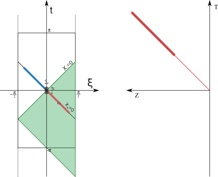
Figure 1: ${AdS}$ in global coordinates with the Poincare patch defined by the horizon $X_{-}=0$ shaded in green. We consider a short string moving in the gray region of linear size $\epsilon$ around $X_{0}=1,\ X_{\pm}=X_{i}=0$. Since the string in nearly massless, after a boost it moves in the red colored region of size $\epsilon^{2}$ around the light-like line $X_{+}=0$, arriving at the horizon at the speed of light. The state in which it falls through the horizon is given by its shape and momentum density and maps directly to the properties of the dual Wilson loop. The Poincare patch (before T-duality) is shown on the right. The string is then almost point-like and moving in a neighborhood of the geodesic indicated in red towards the horizon at $Z=\infty$.

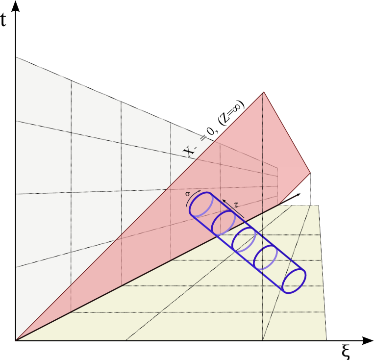
Figure 2: A small boosted (nearly-massless) string falling into the extremal horizon. Let $j_{\sigma,\tau}$ be the components of the current associated with the energy conservation (here $(\tau,\sigma)$ are the world-sheet coordinates). We may compute the energy of the string as an integral in $\sigma$ right at the horizon $\int d\sigma\,j_{\tau}$. Interchanging $\sigma$ and $\tau$, we get a string with a boundary and a flux along the end. The same integral $\int d\tau\,j_{\sigma}$ can be interpreted as a flux of energy leaving the string through the boundary. The two expressions are the same since they are given by the same integral. It is the second interpretation that applies after the T-duality.

At the boundary there is an incoming and outgoing flux of energy. The difference between the fluxes gives the (non-conserved) energy on the open string (Wilson loop) side (see (3.51),(3.53)). On the other hand, the total integrated flux (given by the sum of incoming plus outgoing fluxes) gives the energy of the dual closed string (3.54). For periodic closed string the total integrated incoming and outgoing fluxes are the same (due to level matching) so they contribute equally to the energy. The parameter entering the level matching condition (“wrapping”) is a difference in the momentum flux, and the energy is the sum. They get interchanged after the T-dulaity.

In general, the T-duality is a kind of “position $\leftrightarrow$ momentum” duality (cf. [18]). Here we considered another example making it explicit that the local degrees of freedom (strings) near the horizon are those of the dual momentum theory. A natural expectation is that a string that falls through the horizon should correspond to an insertion of an operator (Wilson loop) in the T-dual theory. Here we have given a precise map for short strings: for a closed string that crosses the horizon we have to insert a Wilson loop with the corresponding shape determined by the shape of the closed string.

More explicitly, suppose we have a process where we send two strings from the boundary (represented by dual operator insertions) which collide in such a way that one outgoing string goes to the boundary (another operator insertion) and the other goes onto the horizon. Then in the dual field theory one has to insert a Wilson loop to represent the latter string. This Wilson loop is precisely the one defined by a wavy line that we discussed. Unfortunately, we do not know at present how to write such a Wilson loop explicitly in terms of the original open string variables, though we have a small closed string description for it.

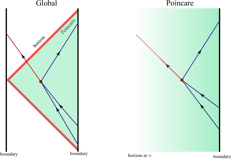
Figure 3: An amplitude with three insertions at the boundary of the Poincare patch and one on the other boundary. The Poincare patch of the ${AdS}$ space in global coordinates is shaded in green. In global coordinates this amplitude is computed by a world-sheet theory with four local operators inserted. In the Poincare patch, the world sheet has a boundary. The boundary conditions, in the T-dual interpretation, are exactly those of a world sheet ending at the boundary of ${AdS}$ space on a line (Wilson loop) with shape and third derivative given by the state of the string falling in. Therefore, from the boundary theory point of view, the amplitude is given by a “mixed” correlator – with three local operator insertions and a non-local Wilson loop of the T-dual “momentum” theory. Although it is not easy to compute it, it is interesting that at least in principle the dual ${\cal N}=4$ gauge theory is self-contained. This is reminiscent of a black hole complementarity but here we are not trying to describe what happens behind the horizon.

In the Euclidean AdS/CFT correspondence, ${\cal N}=4$ Euclidean gauge invariant correlators can be computed as string theory correlators in Euclidean ${AdS}$ for strings that emerge from the boundary by the insertion of appropriate vertex operators. If we consider the Minkowski signature case in global coordinates, the same correspondence applies (see fig. 3). However, when selecting a Poincare patch, it may happen that one (or more) of the local operators inserted in not on the boundary patch, or, equivalently, one (or more) of the closed strings falls into the extremal Poincare horizon. Then the world sheet has a boundary: in the example of fig. 3 the world sheet has three operator insertions plus a boundary at the horizon. In this paper we saw that the conditions at such boundary can be simply expressed by saying that the world sheet ends at a wavy line Wilson loop in the T-dual version of the ${AdS}$ space.

Note that the same ${AdS}$ space can be interpreted as corresponding to the original ${\cal N}=4$ supersymmetric gauge theory or to the T-dual (“momentum”) theory. Therefore, from the dual gauge theory point of view we can compute the same amplitude by replacing the missing local insertion by a Wilson loop of the T-dual “momentum” theory.

The situation is somewhat reminiscent of the black-hole complementarity, although it is not obvious that there is any information about what happens behind the horizon. It should be noted that the present situation corresponds to an (extremal) eternal black hole and therefore the usual paradoxes due to black hole evaporation do not arise. Nevertheless, it is interesting to note that the correlation function can be computed entirely in terms of the operators in a single ${\cal N}=4$ gauge theory. The computation is not straight-forward since the dual (“momentum”) Wilson loop is not easy to represent in terms of the original variables. This is again similar to the complementarity where the missing local operator is scrambled in a non-trivial way when represented in the original variables. Note also that we insert an operator related to the state of the string when crossing the horizon and not directly related to the operator on the other boundary.

6 Discussion

The main result of this paper is the demonstration of existence of a map between the state of a closed string falling into the Poincare horizon and a Wilson loop of the T-dual boundary theory. The T-duality we used is like the one of [18] that relates gluon scattering amplitudes to closed light-like Wilson loops with cusps. In our case the profile of the corresponding Wilson loop is completely determined by the shape of the closed string. In particular, it is periodic with period fixed by the energy of the closed string. This allows us to define correlation functions of local operators where one of the corresponding strings falls into the horizon. The string that crosses the horizon is replaced by a Wilson loop of the T-dual theory.

Our semi-classical computation has barely scratched the surface of what seems to be an interesting topic for further research. For example, these ideas might have implications for understanding the physics of black holes, e.g., black hole complementarity. For example, it suggests that the dynamics of closed strings in a small flat-space region in the bulk of ${AdS}$ is dual to a correlation functions of certain Wilson loops in gauge theory. To make this precise the first step would be to describe the T-duality map at the full quantum level. The algebra of oscillators of the closed string should map to the algebra of the corresponding deformation operators of the Wilson loop. Also, the partition functions of the T-dual world-sheet theories should map to each other, implying that the relation holds to all orders in $\frac{1}{\sqrt{\lambda}}$ expansion.

The T-duality relation discussed above implies that one should be able to translate results known about Wilson loops into statements about closed strings crossing the horizon. In particular, the exact result for the wavy-line open string energy (1.8) should have its counterpart on the small closed string side, potentially providing a link to the slope function in (1.4).

On the dual field theory side, the corresponding problem is how to compute a relation between the spin and the energy radiated by a heavy quark moving along a wavy line trajectory. At lowest order one can phrase this question in the language of [6]. If the period is $\Sigma$, then the quark oscillates with frequency $\omega=\frac{n}{\Sigma}$ ($n$ is a wave number). Let the amplitude of oscillations be $\eta$. According to [6] the quark radiates quanta of energy $\omega$ with probability

$$p_{{}_{\mbox{emission}}}=f(\lambda)\,\omega^{3}|\eta|^{2}\Sigma\ .$$ (6.1)

where $f(\lambda)$ is a known function of $\lambda$ scaling as $\sqrt{\lambda}$ at strong coupling. If those quanta in addition to energy $\omega$ carry spin $1$ (gluons) then the energy and the spin radiated by the quark are

$$E=f(\lambda)\omega^{4}|\eta|^{2}\Sigma\ ,\ \ \ \ \ \ \ \ \ \ \ \ \ \ \ {\rm S}=f(\lambda)\omega^{3}|\eta|^{2}\Sigma\ .$$ (6.2)

It follows then that

$$E=\omega{\rm S}=\frac{n}{\Sigma}{\rm S}\ .$$ (6.3)

Let us now try to interpret this relation in T-dual closed string terms. As we discussed above, the period $\Sigma$ should be proportional (3.14) to the closed-string energy $\Sigma\sim\frac{E}{\sqrt{\lambda}}$. For the open string T-dual to closed string there should be both left and right mover contributions, and the level matching condition implies that the left and right movers emit and absorb the same total energy. Then it follows from (6.3) that

$$E\sim\sqrt{{\sqrt{\lambda}\,n{\rm S}}}\ .$$ (6.4)

This is a Regge trajectory relation for a closed string state at level $N=\tilde{N}={{\textstyle{1\over 2}}}nS$ and tension $\sim\sqrt{\lambda}$. This naive computation should, of course, be made more precise. It is important to understand, for example, how the $1\over\sqrt{\lambda}$ corrections appear.

Appendix A Elliptic Integrals and Jacobi elliptic functions

The rotating string solution and its T-dual are written in terms of Elliptic integrals and Jacobi Elliptic functions. Since there are different notations and definitions used for these functions, especially in the case of an imaginary modulus, in this appendix we briefly collect the definitions that we use, together with some simple properties of these functions. We use the following notation for elliptic integral $\mathbb{E}$

$$\mathbb{E}(\phi,ik)=\int_{0}^{\phi}d\theta\,\sqrt{1+k^{2}\sin^{2}\theta}\,\ .$$ (A.1)

Notice that with this definition $\mathbb{E}$ is an always increasing function; in particular, it is not periodic. This is the appropriate definition for an imaginary modulus. Also we define

$$\mathbf{sn}(z,ik)=\sin\phi(z,ik),\ \ \mathbf{cn}(z,ik)=\cos\phi(z,ik),\ \ \mathbf{dn}(z,ik)=\partial_{z}\phi(z,ik)\ ,$$ (A.2)

where $\phi(z,ik)$ is determined by

$$z=\int_{0}^{\phi(z,ik)}\frac{d\theta}{\sqrt{1+k^{2}\sin^{2}\theta}}\ .$$ (A.3)

Again, for imaginary modulus, $\phi(z,ik)$ is an arbitrary real number and is not a periodic function of $z$. On the other hand, the functions $\mathbf{sn}(z,ik)$, $\mathbf{cn}(z,ik)$ and $\mathbf{dn}(z,ik)$ are periodic. Taking $z$ derivatives on both sides of eq.(A.3) gives

$$\partial_{z}\phi(z,ik)=\sqrt{1+k^{2}\sin^{2}\phi(z,ik)}\ .$$ (A.4)

It follows that

$$\partial_{z}\mathbb{E}\big{(}\phi(z,ik),ik\big{)} = \partial_{z}\phi(z,ik)\sqrt{1+k^{2}\sin^{2}\phi(z,ik)}$$ (A.5)

$$= 1+k^{2}\sin^{2}\phi(z,ik)=1+k^{2}\mathbf{sn}^{2}(z)\ .$$

This implies the following expression for the integral

$$\int\!d\sigma\ \mathbf{sn}^{2}(q\sigma,ik)=-\frac{\sigma}{k^{2}}+\frac{1}{qk^{2}}\mathbb{E}(\mathbf{sn}(q\sigma),ik)\ .$$ (A.6)

Appendix B Spiky string case

Let us consider T-dual of spiky string in ${AdS}$ space [33]. The corresponding flat space solution in the conformal gauge is

$$y_{0} = \tau\ ,\ \ \ \ \ \ \ \ \ \ \ \ \ \ \ \ \ \ \ \ \ \ y_{3}=y_{4}=0\ ,$$

$$y_{1} = \kappa\Big{\{}\cos\Big{[}\frac{\tau+\sigma}{2\kappa}\Big{]}+(n-1)\cos\Big{[}\frac{\tau-\sigma}{2\kappa(n-1)}\Big{]}\Big{\}}\ ,$$

$$y_{2} = \kappa\Big{\{}\sin\Big{[}\frac{\tau+\sigma}{2\kappa}\Big{]}+(n-1)\sin\Big{[}\frac{\tau-\sigma}{2\kappa(n-1)}\Big{]}\Big{\}}\ .$$ (B.1)

Here we choose $y_{0}=\tau$ by rescaling of $\tau$ and $\sigma$, so that $\sigma\equiv\sigma+4\pi\kappa(n-1)$ where $n$ is the number of spikes ($n=2$ is the usual folded spinning string).

This may be viewed as solution in $R^{1,4}$ in the light-cone gauge if we take the advantage of the fact that $y_{4}=0$ and define $y_{\pm}=y_{0}\pm y_{4}=\tau$ (cf. (3.20)). The left and right moving parts of $y_{i}={\rm y}_{i}^{+}(\tau+\sigma)+{\rm y}_{i}^{-}(\tau-\sigma)$ are easily identified as

$${\rm y}_{1}^{+}(\tau)=\kappa\cos\Big{[}\frac{\tau}{2\kappa}\Big{]},\ \ \ \ \ \ \ \ {\rm y}^{-}_{1}(\tau)=\kappa(n-1)\cos\Big{[}\frac{\tau}{2\kappa(n-1)}\Big{]}\ ,$$ (B.2)

$${\rm y}_{2}^{+}(\tau)=\kappa\sin\Big{[}\frac{\tau}{2\kappa}\Big{]},\ \ \ \ \ \ \ \ {\rm y}^{-}_{2}(\tau)=\kappa(n-1)\sin\Big{[}\frac{\tau}{2\kappa(n-1)}\Big{]}\ .$$ (B.3)

The corresponding open string (Wilson loop) data follows from the general expression for the T-dual solution in section 3 (see (3.31)). After the redefinition $\sigma\leftrightarrow\tau$ we get

$${\cal T} = \tau\ ,$$ (B.4)

$${\cal X}_{1} = 2\kappa\epsilon\Big{\{}\sin\Big{[}\frac{\tau}{2\kappa}\Big{]}+(n-1)^{2}\sin\Big{[}\frac{\tau}{2\kappa(n-1)}\Big{]}\Big{\}}\ ,$$ (B.5)

$${\cal X}_{2} = -2\kappa\epsilon\Big{\{}\cos\Big{[}\frac{\tau}{2\kappa}\Big{]}-(n-1)^{2}\cos\Big{[}\frac{\tau}{2\kappa(n-1)}\Big{]}\Big{\}}\ ,$$ (B.6)

$$\partial_{\sigma}^{3}{\cal X}_{1} = \frac{\epsilon}{2\kappa}\Big{\{}\cos\Big{[}\frac{\tau}{2\kappa}\Big{]}-\frac{1}{n-1}\cos\Big{[}\frac{\tau}{2\kappa(n-1)}\Big{]}\Big{\}}\ ,$$ (B.7)

$$\partial_{\sigma}^{3}{\cal X}_{2} = \frac{\epsilon}{2\kappa}\Big{\{}\sin\Big{[}\frac{\tau}{2\kappa}\Big{]}+\frac{1}{n-1}\sin\Big{[}\frac{\tau}{2\kappa(n-1)}\Big{]}\Big{\}}\ .$$ (B.8)

The modulus of the acceleration of the end point of the open string (quark) is given by

$$a^{2}=(\partial_{\tau}^{2}{\cal X}_{1})^{2}+(\partial_{\tau}^{2}{\cal X}_{2})^{2}=\frac{\epsilon^{2}}{\kappa^{2}}\sin^{2}\Big{[}\frac{n\tau}{4(n-1)\kappa}\Big{]}\ .$$ (B.9)

The acceleration vanishes at the points

$$\tau_{m}=4\kappa\pi\frac{n-1}{n}\,m,\ \ \ \ \ \ \ \ \ \ \ \ m\in\mathbb{Z}\ .$$ (B.10)

These correspond to the positions of the cusps on the small spiky string side, i.e. the cusps of the small string are seen in the T-dual picture as the points where the acceleration of the end-point quark vanishes.

Note that if the Wilson loop had cusps itself (namely, jumps in the velocity) then the corresponding small string would have jumps in the position. This is not possible, i.e. one cannot obtain Wilson loops with cusps by this T-duality transform. In fact, it was already argued in [18] that the cusped Wilson loops are dual to open strings representing scattering of gluons (i.e. to non gauge-invariant operators).

Appendix C T-duality in a non-compact direction on a cylinder

The world-sheet theory corresponding to the closed string is defined on the cylinder (see fig. 2). At the same time, the coordinates ${\cal X}_{\mu}$ that we T-dualized in (2.13),(3.23) are non-compact and that may be a source of concern. Below we shall review the application of T-duality in such a case of a non-compact target space coordinate (we shall consider only one bosonic ${\cal X}_{0}={\cal T}$ coordinate). The fermionic T-duality and the full quantum map in the case of the $AdS_{5}\times S^{5}$ superstring theory is left for the future work.

The generic world-sheet action can be written as (we ignore the overall factor of string tension)

$$S=\int d\sigma d\tau\Big{[}g_{{\cal T}{\cal T}}(\partial_{\tau}{\cal T}\partial_{\tau}{\cal T}-\partial_{\sigma}{\cal T}\partial_{\sigma}{\cal T})+2g_{{\cal T}i}(\partial_{\tau}{\cal T}\partial_{\tau}{\cal X}^{i}-\partial_{\sigma}{\cal T}\partial_{\sigma}{\cal X}^{i})$$

$$\ \ \ \ \ \ \ \ \ \ \ \ \ \ \ \ \ \ \ \ +\ g_{ij}(\partial_{\tau}{\cal X}^{i}\partial_{\tau}{\cal X}^{j}-\partial_{\sigma}{\cal X}^{i}\partial_{\sigma}{\cal X}^{j})\Big{]}\ ,$$ (C.1)

where in our present case the metric depends only on the coordinate $Z$ that is not displayed here. Gauging as usual the shifts in ${\cal T}$ we get

$$S = \int d\sigma d\tau\Big{[}g_{{\cal T}{\cal T}}(A_{\tau}A_{\tau}-A_{\sigma}A_{\sigma})+2g_{{\cal T}i}(A_{\tau}\partial_{\tau}{\cal X}^{i}-A_{\sigma}\partial_{\sigma}{\cal X}^{i})+g_{ij}(\partial_{\tau}{\cal X}^{i}\partial_{\tau}{\cal X}^{j}-\partial_{\sigma}{\cal X}^{i}\partial_{\sigma}{\cal X}^{j})$$ (C.2)

$$\ \ \ \ \ \ \ \ \ \ \ \ \ \ \ \ \ +\ \tilde{{\cal T}}(\partial_{\sigma}A_{\tau}-\partial_{\tau}A_{\sigma})\Big{]}\ .$$

The path integral over the Lagrange multiplier $\tilde{{\cal T}}$ enforces $A_{\sigma,\tau}$ to be a pure gauge and therefore the path integral over $\tilde{{\cal T}},A_{\sigma},A_{\tau}$ is equivalent to the path integral over ${\cal T}$. On the other hand, integrating first over $A_{\sigma}$, $A_{\tau}$ gives the T-dual action for $\tilde{{\cal T}}$.

To deal with the subtetly of the theory defined on the cylinder let us expand all the variables as periodic functions of $\sigma$ (here assumed to be $2\pi$ periodic)

$${\cal T} = \xi_{0}(\tau)+\sum_{n\neq 0}e^{in\sigma}\xi_{n}(\tau)\ ,\ \ \ \ \ \ \ \ \ \ \ \ \ \ \ \tilde{{\cal T}}=\tilde{\xi}_{0}(\tau)+\sum_{n\neq 0}e^{in\sigma}\tilde{\xi}_{n}(\tau)\ ,$$ (C.3)

$$A_{\sigma} = \xi_{\sigma 0}(\tau)+\sum_{n\neq 0}e^{in\sigma}\xi_{\sigma n}(\tau)\ ,\ \ \ \ \ \ \ \ \ \ \ \ \ A_{\tau}=\xi_{\tau 0}(\tau)+\sum_{n\neq 0}e^{in\sigma}\xi_{\tau n}(\tau)\ .$$ (C.4)

Ignoring first the zero modes, let us check that the path integral over $\xi_{\sigma n}(\tau)$, $\xi_{\tau n}(\tau)$ and $\tilde{\xi}_{n}(\tau)$ is equivalent to the path integral over $\xi_{n}(\tau)$. Indeed, the action has a term

$$\int d\tau\sum_{n\neq 0}\tilde{\xi}_{-n}(in\xi_{\tau n}-\partial_{\tau}\xi_{\sigma n})\ .$$ (C.5)

The path integral over $\tilde{\xi}_{n}$ enforces the relation $\xi_{\tau n}=\frac{1}{in}\partial_{\tau}\xi_{\sigma n}$ which means that the only independent variables remaining are $\xi_{\sigma n}$. Then defining $\xi_{n}=\frac{1}{in}\xi_{\sigma n}$ accomplishes the task.

The zero modes in (C.3),(C.4) present, however, few problems. Notice that $\xi_{\tau 0}$ which should be equal to $\partial_{\tau}\xi_{0}$ does not appear in the last term

$$S_{A}=\int d\tau d\sigma\,\tilde{{\cal T}}(\partial_{\sigma}A_{\tau}-\partial_{\tau}A_{\sigma})$$ (C.6)

in the action (C.2). To enforce the required relation we may add an extra term to the action depending on a new variable $\mu_{0}(\tau)$

$$S_{0}=-\int d\tau\ \mu_{0}(\tau)(\xi_{\tau 0}-\partial_{\tau}\xi_{0})=-{1\over 2\pi}\int d\tau d\sigma\ \mu_{0}(\tau)A_{\tau}+\int d\tau\ \mu_{0}(\tau)\partial_{\tau}\xi_{0}\ .$$ (C.7)

Performing the path integral over $\mu_{0}(\tau)$ gives $\xi_{\tau 0}=\partial_{\tau}\xi_{0}$ and the subsequent integral over $\xi_{0}$ completes the ${\cal T}$ with the zero mode. Integrating by parts in the last term of (C.7) gives

$$S_{0}=-{1\over 2\pi}\int d\tau d\sigma\ \mu_{0}(\tau)A_{\tau}-\int d\tau\ \partial_{\tau}\mu_{0}(\tau)\xi_{0}(\tau)+\mu_{0}(\tau_{f})\xi_{0}(\tau_{f})-\mu_{0}(\tau_{i})\xi_{0}(\tau_{i})\ .$$ (C.8)

If we now integrate over $\xi_{0}$ we get $\mu_{0}=$const. Adding together the extra $S_{A}$ and $S_{0}$ terms and after some integral by parts, we have

$$S_{A}+S_{0}=-\int d\tau d\sigma\ \Big{[}(\partial_{\sigma}\tilde{{\cal T}}+\bar{\mu}_{0})A_{\tau}-\partial_{\tau}\tilde{{\cal T}}A_{\sigma}\Big{]}+2\pi\bar{\mu}_{0}[\xi_{0}(\tau_{f})-\xi_{0}(\tau_{i})]\ ,\ \ \ \ \ \ \ \ \ \ \bar{\mu}={1\over 2\pi}\mu_{0}\ .$$ (C.9)

In the T-dual action we should replace $\partial_{\sigma}\tilde{{\cal T}}\rightarrow\partial_{\sigma}\tilde{{\cal T}}+\bar{\mu}_{0}$.

If we Fourier transform over the center of mass positions $\xi_{0}(\tau_{f})$ and $\xi_{0}(\tau_{i})$ we get that the initial and final momenta in the ${\cal T}$ direction should be equal to $\mu_{0}$. Therefore, instead of integrating over $\mu_{0}$ we can fix $\mu_{0}$ to be equal to the value of the corresponding conserved momentum, namely, the energy conjugate to ${\cal T}={\cal X}_{0}$.

Up to now we discussed the theory defined on the cylinder with all the functions periodic in $\sigma$. However, we may formally define the T-dual coordinate $\tilde{{\cal T}}$ as

$$\tilde{{\cal T}}=\bar{\mu}_{0}\sigma+\sum_{n\neq 0}\tilde{\xi}_{n}(\tau)e^{in\sigma}\ .$$ (C.10)

Including the linear term in $\sigma$ is allowed as $\tilde{{\cal T}}$ enters in the action through its derivatives which are all periodic. A problem, however, arises if we insert vertices with momenta in the direction of $\tilde{{\cal T}}$: the presence of a factor $\exp(i\tilde{E}\tilde{{\cal T}})$ will break the periodicity in $\sigma$.

Equivalently, we may consider the coordinate $\tilde{{\cal T}}$ to be periodic with period determined by the energy, $\tilde{{\cal T}}\equiv\tilde{{\cal T}}+2\pi E$. Physically, the period changes with the energy so it should not be considered a property of the dual space-time but of the configuration that we are considering. The T-dual string surface is then an open string world sheet which is periodic along $\tilde{{\cal T}}$.

Another problem is that the zero mode part of the Lagrange multiplier term (C.6)

$$S_{A0}=\int d\tau\ \tilde{\xi}_{0}(\tau)\partial_{\tau}\xi_{\sigma n}(\tau)$$ (C.11)

sets $\partial_{\tau}\xi_{\sigma n}(\tau)=0$ as it should, but leaves a possible zero mode $\xi_{\tau 0}$ independent of $\tau$. The latter implies the presence of a term ${\cal T}\sim\xi_{\tau 0}\sigma$ which should not be allowed by the periodicity. This can be dealt with by setting it to zero with a Lagrange multiplier.

References

- [1] S. S. Gubser, I. R. Klebanov and A. M. Polyakov, “A Semiclassical limit of the gauge / string correspondence,” Nucl. Phys. B 636, 99 (2002) [hep-th/0204051].
- [2] M. Kruczenski, “A Note on twist two operators in N=4 SYM and Wilson loops in Minkowski signature,” JHEP 0212, 024 (2002) [hep-th/0210115].
- [3] M. Kruczenski, R. Roiban, A. Tirziu and A. A. Tseytlin, “Strong-coupling expansion of cusp anomaly and gluon amplitudes from quantum open strings in AdS(5) x S5,” Nucl. Phys. B 791, 93 (2008) [arXiv:0707.4254 [hep-th]].
- [4] L. F. Alday, D. Gaiotto, J. Maldacena, A. Sever and P. Vieira, “An Operator Product Expansion for Polygonal null Wilson Loops,” JHEP 1104, 088 (2011) [arXiv:1006.2788 [hep-th]].
- [5] L. F. Alday, B. Eden, G. P. Korchemsky, J. Maldacena and E. Sokatchev, “From correlation functions to Wilson loops,” JHEP 1109, 123 (2011) [arXiv:1007.3243 [hep-th]].
- [6] D. Correa, J. Henn, J. Maldacena and A. Sever, “An exact formula for the radiation of a moving quark in N=4 super Yang Mills,” JHEP 1206, 048 (2012) [arXiv:1202.4455].
- [7] J. K. Erickson, G. W. Semenoff and K. Zarembo, “Wilson loops in N=4 supersymmetric Yang-Mills theory,” Nucl. Phys. B 582, 155 (2000) [hep-th/0003055].
- [8] N. Gromov and A. Sever, “Analytic Solution of Bremsstrahlung TBA,” arXiv:1207.5489 [hep-th].
- [9] B. Basso, “An exact slope for AdS/CFT,” arXiv:1109.3154 [hep-th].
- [10] N. Gromov, “On the Derivation of the Exact Slope Function,” arXiv:1205.0018 [hep-th].
- [11] B. Basso, “Scaling dimensions at small spin in N=4 SYM theory,” arXiv:1205.0054 [hep-th].
- [12] M. Beccaria and A. A. Tseytlin, “More about ’short’ spinning quantum strings,” JHEP 1207, 089 (2012) [arXiv:1205.3656 [hep-th]].
- [13] B. Fiol, B. Garolera and A. Lewkowycz, “Exact results for static and radiative fields of a quark in N=4 super Yang-Mills,” JHEP 1205, 093 (2012) [arXiv:1202.5292 [hep-th]].
- [14] A. M. Polyakov and V. S. Rychkov, “Gauge field strings duality and the loop equation,” Nucl. Phys. B 581, 116 (2000) [hep-th/0002106].
- [15] G. W. Semenoff and D. Young, “Wavy Wilson line and AdS / CFT,” Int. J. Mod. Phys. A 20, 2833 (2005) [hep-th/0405288].
- [16] A. Mikhailov, “Nonlinear waves in AdS / CFT correspondence,” hep-th/0305196.
- [17] R. Kallosh and A. A. Tseytlin, “Simplifying superstring action on AdS(5) x S5,” JHEP 9810, 016 (1998) [hep-th/9808088].
- [18] L. F. Alday and J. M. Maldacena, “Gluon scattering amplitudes at strong coupling,” JHEP 0706, 064 (2007) [arXiv:0705.0303 [hep-th]].
- [19] R. Ricci, A. A. Tseytlin and M. Wolf, “On T-Duality and Integrability for Strings on AdS Backgrounds,” JHEP 0712, 082 (2007) [arXiv:0711.0707].
- [20] N. Berkovits and J. Maldacena, “Fermionic T-Duality, Dual Superconformal Symmetry, and the Amplitude/Wilson Loop Connection,” JHEP 0809, 062 (2008) [arXiv:0807.3196].
- [21] N. Beisert, R. Ricci, A.A. Tseytlin and M. Wolf, “Dual Superconformal Symmetry from AdS(5) x S5 Superstring Integrability,” Phys. Rev. D 78, 126004 (2008) [arXiv:0807.3228].
- [22] S. Frolov and A. A. Tseytlin, “Semiclassical quantization of rotating superstring in AdS(5) x S5,” JHEP 0206, 007 (2002) [hep-th/0204226].
- [23] H. Hayashi, K. Okamura, R. Suzuki and B. Vicedo, “Large Winding Sector of AdS/CFT,” JHEP 0711, 033 (2007) [arXiv:0709.4033 [hep-th]].
- [24] D. Correa, J. Maldacena and A. Sever, “The quark anti-quark potential and the cusp anomalous dimension from a TBA equation,” JHEP 1208, 134 (2012) [arXiv:1203.1913 [hep-th]].
- [25] N. Drukker, “Integrable Wilson loops,” arXiv:1203.1617 [hep-th].
- [26] M. Beccaria, G. V. Dunne, V. Forini, M. Pawellek and A. A. Tseytlin, “Exact computation of one-loop correction to energy of spinning folded string in AdS5 x S5,” J. Phys. A 43, 165402 (2010) [arXiv:1001.4018 [hep-th]].
- [27] I.S. Gradshteyn and I.M. Ryzhik, “Table of Integrals, Series and Products”. Academic Press Inc. (2007).
- [28] D. E. Berenstein, R. Corrado, W. Fischler and J. M. Maldacena, “The Operator product expansion for Wilson loops and surfaces in the large N limit,” Phys. Rev. D 59 (1999) 105023 [hep-th/9809188].
- [29] N. Drukker, D. J. Gross and H. Ooguri, “Wilson loops and minimal surfaces,” Phys. Rev. D 60 (1999) 125006 [hep-th/9904191].
- [30] J. K. Erickson, G. W. Semenoff and K. Zarembo, “Wilson loops in N=4 supersymmetric Yang-Mills theory,” Nucl. Phys. B 582, 155 (2000) [hep-th/0003055]. N. Drukker and D. J. Gross, “An Exact prediction of N=4 SUSYM theory for string theory,” J. Math. Phys. 42, 2896 (2001) [hep-th/0010274]. V. Pestun, “Localization of gauge theory on a four-sphere and supersymmetric Wilson loops,” Commun. Math. Phys. 313, 71 (2012) [arXiv:0712.2824].
- [31] N. Drukker and V. Forini, “Generalized quark-antiquark potential at weak and strong coupling,” JHEP 1106, 131 (2011) [arXiv:1105.5144].
- [32] M. Chernicoff and A. Guijosa, “Acceleration, Energy Loss and Screening in Strongly-Coupled Gauge Theories,” JHEP 0806, 005 (2008) [arXiv:0803.3070 [hep-th]]. M. Chernicoff, J. A. Garcia and A. Guijosa, “A Tail of a Quark in N=4 SYM,” JHEP 0909, 080 (2009) [arXiv:0906.1592 [hep-th]].
- [33] M. Kruczenski, “Spiky strings and single trace operators in gauge theories,” JHEP 0508, 014 (2005) [hep-th/0410226].
- [34] R. Roiban, A. Tirziu and A. A. Tseytlin, “Slow-string limit and ’antiferromagnetic’ state in AdS/CFT,” Phys. Rev. D 73, 066003 (2006) [hep-th/0601074].