Explicit-Implicit Scheme for Relativistic Radiation Hydrodynamics

Abstract

We propose an explicit-implicit scheme for numerically solving Special Relativistic Radiation Hydrodynamic (RRHD) equations, which ensures a conservation of total energy and momentum (matter and radiation). In our scheme, 0th and 1st moment equations of the radiation transfer equation are numerically solved without employing a flux-limited diffusion (FLD) approximation. For an hyperbolic term, of which the time scale is the light crossing time when the flow velocity is comparable to the speed of light, is explicitly solved using an approximate Riemann solver. Source terms describing an exchange of energy and momentum between the matter and the radiation via the gas-radiation interaction are implicitly integrated using an iteration method. The implicit scheme allows us to relax the Courant-Friedrichs-Lewy condition in optically thick media, where heating/cooling and scattering timescales could be much shorter than the dynamical timescale. We show that our numerical code can pass test problems of one- and two-dimensional radiation energy transport, and one-dimensional radiation hydrodynamics. Our newly developed scheme could be useful for a number of relativistic astrophysical problems. We also discuss how to extend our explicit-implicit scheme to the relativistic radiation magnetohydrodynamics.

1. Introduction

Relativistic flows appear in many high-energy astrophysical phenomena, such as jets from microquasars and active galactic nuclei (AGNs), pulsar winds, magnetar flares, core collapse supernovae, and gamma-ray bursts (GRBs). In many of these systems, the magnetic field has a crucial role in dynamics. For example, magnetic fields connecting an accretion disk with a central star, or, different points of accretion disks are twisted and amplified due to the differential rotation, launching the jets (Lovelace, 1976; Blandford & Payne, 1982; Uchida & Shibata, 1985). The production of astronomical jets has been observed in magnetohydrodynamic (MHD) simulations (Hayashi et al., 1996; Meier et al., 2001; Kato et al., 2004). The jets are also powered by a subtraction of the rotational energy of a central black hole via the magnetic field (Blandford & Znajek, 1977; Koide et al., 2002; McKinney & Blandford, 2009). Also the magnetic fields play an important role in accretion disks to transport the angular momentum outward, leading to the mass accretion (Balbus & Hawley, 1991; Hawley et al., 1995)

Not merely the observational point of view, but the radiation field is also an important ingredient in the dynamics of relativistic phenomena. The radiation pressure force would play a key role in jet acceleration (Bisnovatyi-Kogan & Blinnikov, 1977; Sikora et al., 1996; Ohsuga et al., 2005; Okuda et al., 2009). Recently, Takeuchi et al. (2010) showed a formation of radiatively accelerated and magnetically collimated jets using non-relativistic radiation MHD (RMHD) simulations (see also Ohsuga et al., 2009; Ohsuga & Mineshige, 2011). The radiative effect also plays important roles in non-relativistic phenomena. For example, the dominance of the radiation pressure in optically thick, geometrically thin (standard) accretion disks could be unstable to thermal and viscous instabilities (Lightman & Eardley, 1974; Shibazaki & Hōshi, 1975; Shakura & Sunyaev, 1976; Takahashi & Masada, 2011). Here we note that the global radiation hydrodynamic (RHD) simulations showed the growth of instabilities (Ohsuga, 2006), but Hirose et al. (2009) concluded that the radiation pressure dominated region is thermally stable using RMHD simulations of a local patch of the disk. Thus the high energy phenomena would be understood only after we take into account the magnetic field and the radiation consistently.

Many methods have been proposed to include radiative effects in non-relativistic plasmas. Solving a full radiation transfer equation is the most challenging task for directly connecting results between numerical simulations and observations (Stone et al., 1992). But it is a hard task to couple with the hydrodynamical code due to its complexity and high computational costs. Another class of simple method is based on the moment method. In the Flux-Limited Diffusion approximation (FLD), a 0th moment equation of the radiation transfer equation is solved to evaluate the radiation energy density, $E^{\prime}_{r}$. The radiative flux, $\mbox{\boldmath$F$}^{\prime}_{r}$, is given based on the gradient of the radiation energy density without solving the 1st moment equation. This is quite a useful technique and gives appropriate radiation fields within the optically thick regime, but we should keep in mind that it does not always give precise radiation fields in the regime where the optical depth is around unity or less (see Ohsuga & Mineshige, 2011). Thus it is better to solve the 0th and 1st moment equations.

When we solve two moment equations, the closure relation, $P^{\prime ij}_{r}=D^{ij}E_{r}^{\prime}$, is used to evaluate the radiation stress, $P_{r}^{\prime ij}$, where $D^{ij}$ is the Eddington tensor. In the Eddington approximation, the tensor is simply given by $D^{ij}=\delta^{ij}/3$, where $\delta^{ij}$ is the Kronecker delta. This implies that the radiation field is isotropic in the comoving frame, which is a reasonable assumption in the optically thick media. Another class of the Eddington tensor is obtained by approximately taking into account the anisotropy of radiation fields (so called M-1 closure, Kershaw, 1976; Minerbo, 1978; Levermore, 1984). González et al. (2007) implemented the M-1 closure in their non-relativistic hydrodynamic code and demonstrated that the anisotropic radiation fields around an obstacle are accurately solved.

In the framework of relativistic radiation hydrodynamics (RRMHD), Farris et al. (2008) first proposed a numerical scheme for solving general relativistic radiation magnetohydrodynamic equations assuming an optically thick medium (i.e., $D^{ij}=\delta^{ij}/3$). Zanotti et al. (2011) implemented the general relativistic radiation hydrodynamics code and adopted it for the Bondi-Hoyle accretion on to the black hole. Recently, Shibata et al. (2011) proposed another truncated moment formalism of radiation fields in optically thick and thin limits.

In the RR(M)HD, there are three independent timescales. The first one is the dynamical time scale $t_{dyn}\equiv L/v$, where $L$ and $v$ are the typical size of the system and the fluid velocity. The second one is the timescale at which the characteristic wave passes the system, $t_{w}\equiv L/\lambda$, where $\lambda$ is the characteristic wave speed. These two timescales are comparable and close to the light crossing time, $L/c$ (where $c$ is the speed of light) in relativistic phenomena (i.e., $v\sim\lambda\sim c$). The third one is the heating/cooling and scattering timescales, $t_{\rm ab}$ and $t_{\rm sc}$. These timescales become much shorter than the dynamical one in the optically thick medium, since the gas and the radiation are frequently interact. This indicates that equations for the radiation fields become stiff. In the explicit scheme, a numerical time step $\Delta t$ should be restricted to being shorter than these typical timescales ($\Delta t<\min[t_{dyn},t_{w},t_{ab},t_{sc}]$) to ensure the numerical stability. Therefore, high computational costs prevent us from studying long term evolutions when the gas is optically thick, if we are interested in the phenomena of the dynamical timescale.

In this paper, we propose an explicit-implicit numerical scheme overcome this problem. As the first step, we consider the relativistic radiation hydrodynamics by neglecting the magnetic field (but, see section 5 for the discussion how to extend our numerical scheme to RRMHD). The proposed scheme ensures a conservation of total energy and momentum. Governed equations are integrated in time using both explicit and implicit schemes. The former solves an hyperbolic term (timescale $\sim t_{w}\sim t_{dyn}$). The latter treats the exchange of energy and momentum between the radiation and the matter via the gas-radiation interaction, whose time scales are $\sim t_{ab}$ and $t_{sc}$. This method allows us to take a larger time step $\Delta t>t_{ab},t_{sc}$ than that of the explicit scheme.

This paper is organized as follows: In § 2, we introduce argument equations for RRHD and the numerical scheme is shown in § 3. Numerical results of one- and two-dimensional tests are shown in § 4. Discussion and summary are appeared in § 5 and § 6.

2. Basic Equations

In the following, we take the light speed as unity. The special relativistic radiation magnetohydrodynamic equations of ideal gas consist of conservation of mass,

$$(\rho u^{\nu})_{,\nu}=0,$$ (1)

conservation of energy-momentum,

$$\left(T^{\mu\nu}_{\mathrm{HD}}+T^{\mu\nu}_{\mathrm{rad}}\right)_{,\nu}=0,$$ (2)

and equations of radiation energy-momentum

$$T^{\mu\nu}_{\mathrm{rad,\nu}}=-G^{\mathrm{\mu}},$$ (3)

where $\rho$ is the proper mass density, $u^{\mu}=\gamma(1,v^{i})$ is the fluid four velocity, and $T^{\mu\nu}_{\mathrm{HD}}$ and $T^{\mu\nu}_{\mathrm{rad}}$ are energy momentum tensors of fluid and radiation. Here $\gamma=\sqrt{1+u_{i}u^{i}}$ is the bulk Lorentz factor and $v^{i}$ is the fluid three velocity. Greek indices range over $0,1,2,3$ and Latin ranges over $1,2,3$, where $0$ indicates the time component and $1,2,3$ do space components.

The energy momentum tensor of fluids is written as

$$T^{\mu\nu}_{\mathrm{HD}}=\rho\xi u^{\mu}u^{\nu}+p_{g}\eta^{\mu\nu},$$ (4)

where $p_{g}$ is the gas pressure and $\mathrm{diag}~{}\eta^{\mu\nu}=(-1,1,1,1)$ is the Minkowski metric. The specific enthalpy of relativistic ideal gas $\xi$ is given by

$$\xi=1+\frac{\Gamma}{\Gamma-1}\frac{p_{g}}{\rho},$$ (5)

where $\Gamma$ is the specific heat ratio.

The energy momentum tensor of radiation is written as

$$T^{\mu\nu}_{\mathrm{rad}}=\left(\begin{array}[]{cc}E_{r},&F_{r}^{j}\\ F_{r}^{i},&P^{ij}_{r}\end{array}\right)$$ (6)

where $E_{r}$, $F_{r}^{i}$, and $P^{ij}_{r}$ are the radiation energy density, flux and stress measured in the laboratory frame.

The radiation exchanges its energy and momentum with fluids through absorption/emission and scattering processes. The radiation four force $G^{\mu}$ is explicitly given by

$$G^{0} = -\rho\kappa\left(4\pi\mathrm{B}\gamma-\gamma E_{r}+u_{i}F_{r}^{i}\right)$$ (7)

$$- \rho\sigma_{s}\left[\gamma u^{2}E_{r}+\gamma u_{i}u_{j}P^{ij}_{r}-\left(\gamma^{2}+u^{2}\right)u_{i}F_{r}^{i}\right],$$

and

$$G^{i} = -4\pi\rho\kappa\mathrm{B}u^{i}+\rho(\kappa+\sigma_{s})(\gamma F_{r}^{i}-u_{j}P^{ij}_{r})$$ (8)

$$- \rho\sigma_{s}u^{i}\left(\gamma^{2}E_{r}-2\gamma u_{j}F_{r}^{j}+u_{j}u_{k}P_{r}^{jk}\right),$$

where $u=\sqrt{u_{i}u^{i}}$. $\kappa$ and $\sigma_{s}$ are absorption and scattering coefficients measured in the comoving frame. Thus, equation (3) is a mixed-frame radiation energy-momentum equation that the radiation field is defined in the observer frame, while the absorption and scattering coefficients are defined in the comoving frame.

In equations (7) and (8), we assume the Kirchhoff-Planck relation so that the emissivity $\eta$ is replaced by the blackbody intensity $\mathrm{B}$ as $\eta=\kappa\mathrm{B}$ in the comoving frame.

The blackbody intensity $\mathrm{B}$ is a function of gas temperature $T$ as $\mathrm{B}=a_{R}T^{4}/(4\pi)$, where $a_{R}$ is related to the Stefan-Boltzmann constant $\sigma_{\mathrm{SB}}=a_{R}/4$. The plasma temperature is determined by

$$p_{g}=\frac{\rho k_{B}T}{\mu m_{p}},$$ (9)

where $k_{B}$ and $m_{p}$ are the Boltzmann constant and the proton mass, and $\mu$ is the mean molecular weight.

Since we consider the moment equation of radiation fields, we need another relation between $E_{r}$, $F_{r}^{i}$ and $P_{r}^{ij}$ to close the system, i.e., the closure relation. Here we leave it as a general form described by

$$P^{\prime ij}_{r}=P^{\prime ij}(E_{r}^{\prime},F_{r}^{\prime k}),$$ (10)

where dash denotes the quantity defined in the comoving frame. The explicit form of closure relation is introduced in § 3.3 after the formulation.

In the following, we deal with the one-dimensional conservation law in the $x$-direction:

$$\frac{\partial\mathcal{U}}{\partial t}+\frac{\partial\mathcal{F}}{\partial x}=\mathcal{S},$$ (11)

which follows equations (1), (2), and (3). Primitive variables $\mathcal{P}$ are defined as

$$\mathcal{P}=\left(\begin{array}[]{c}\rho\\ u^{k}\\ p_{g}\\ E_{r}\\ F_{r}^{k}\\ \end{array}\right).$$ (12)

Conserved variables $\mathcal{U}$, fluxes $\mathcal{F}$, and source terms $\mathcal{S}$ have forms of

$$\mathcal{U}=\left(\begin{array}[]{c}D\\ m_{t}^{k}\\ E_{t}\\ E_{r}\\ F_{r}^{k}\\ \end{array}\right),$$ (13)

$$\mathcal{F}=\left(\begin{array}[]{c}Dv^{x}\\ \rho\xi u^{x}u^{k}+p_{g}\delta^{xk}+P_{r}^{xk}\\ m_{t}^{x}\\ F_{r}^{x}\\ P_{r}^{xk}\end{array}\right),$$ (14)

and

$$\mathcal{S}\equiv\left(\begin{array}[]{c}0\\ 0\\ 0\\ S_{E}\\ S_{F}^{k}\\ \end{array}\right)=\left(\begin{array}[]{c}0\\ 0\\ 0\\ -G^{0}\\ -G^{k}\\ \end{array}\right),$$ (15)

where $D=\rho\gamma$ is the mass density measured in the laboratory frame. The total energy density $E_{t}$ and momentum density $m_{t}$ are given by

$$E_{t}=E_{\mathrm{HD}}+E_{r}=\rho\xi\gamma^{2}-p_{g}+E_{r},$$ (16)

and

$$m^{k}_{t}=m^{k}_{\mathrm{HD}}+F_{r}^{k}=\rho\xi\gamma u^{k}+F_{r}^{k},$$ (17)

where $E_{\mathrm{HD}}$ and $m^{k}_{\mathrm{HD}}$ denote the energy and momentum density of the fluids, respectively.

It should be noted that $E_{r}$ and $F_{r}^{k}$ are not only the primitive variables, but also the conserved variables. Thus, it is straightforward for the radiation fields to convert the primitive variables from the conserved variables, as we will see in § 3.2.

3. Numerical Scheme for RRHD

In this section, we propose a new numerical scheme for solving RRHD equations. A conservative discretization of 1-dimensional equation (11) over a time step $\Delta t$ from $t=n\Delta t$ to $t=(n+1)\Delta t$ with grid spacing $\Delta x$ is written as

$$\mathcal{U}^{n+1}_{i}=\mathcal{U}^{n}_{i}-\frac{\Delta t}{\Delta x}\left(f_{i+\frac{1}{2}}-f_{i-\frac{1}{2}}\right)+\mathcal{S}_{i}\Delta t,$$ (18)

where $\mathcal{U}^{n}_{i}$ is the conservative variable at $x=x_{i}$ and $t=n\Delta t$, and $f_{i\pm\frac{1}{2}}$ is the upwind numerical flux at the cell surfaces $x=x_{i\pm\frac{1}{2}}$. In the numerical procedure, we divide equation (18) into two parts, the hyperbolic term

$$\mathcal{U}^{*}_{i}=\mathcal{U}^{n}_{i}-\frac{\Delta t}{\Delta x}\left(f_{i+\frac{1}{2}}-f_{i-\frac{1}{2}}\right),$$ (19)

and the source term

$$\mathcal{U}^{n+1}_{i}=\mathcal{U}^{*}_{i}+\mathcal{S}_{i}\Delta t,$$ (20)

where $\mathcal{U}^{*}$ is the conservative variable at the auxiliary step. In the following subsection, we describe how to solve these two equations.

3.1. hyperbolic term

For the hyperbolic term, equation (19) is solved as an initial value problem with the initial condition

$$\mathcal{U}(t^{n},x)=\left\{\begin{array}[]{lll}\mathcal{U}_{L}&\mathrm{for}&x<x_{i+\frac{1}{2}}\\ \mathcal{U}_{R}&\mathrm{for}&x>x_{i+\frac{1}{2}}\end{array}\right.$$ (21)

where the subscript $L$ and $R$ denote left and right constant states on the cell interface. When we take $\mathcal{U}_{L}=\mathcal{U}_{i}$ and $\mathcal{U}_{R}=\mathcal{U}_{i+1}$, the numerical solution is reliable with a first order accuracy in space.

In order to improve the spatial accuracy, primitive variables at the zone surface $\mathcal{P}_{i\pm 1/2}$ are calculated by interpolating them from a cell center to a cell surface (the so-called reconstruction step). The primitive variables at the left and right states are written as

$$\mathcal{P}_{i\pm\frac{1}{2},S}=\mathcal{P}_{i}\pm\frac{\delta_{x}\mathcal{P}}{2},$$ (22)

where we take $S=L(R)$ with the plus (minus) sign. The slope $\delta_{x}P$ should be determined so as to preserve the monotonicity. In our numerical code, we adopt the harmonic mean proposed by van Leer (1977), which has a 2nd order accuracy in space, as

$$\delta_{x}\mathcal{P}=\frac{2\mathrm{max(0,\Delta\mathcal{P}_{+}\Delta\mathcal{P}_{-})}}{\Delta\mathcal{P}_{+}+\Delta\mathcal{P}_{-}},$$ (23)

where

$$\Delta\mathcal{P}_{\pm}=\pm(\mathcal{P}_{i\pm 1}-\mathcal{P}_{i}).$$ (24)

Here we adopted a 2nd order accurate scheme, but a higher order scheme such as Piecewise Constant Method (Komissarov, 1999), Piecewise Parabolic Method (Colella & Woodward, 1984; Martí & Mueller, 1996) or the other scheme can be applicable to both hydropart and radiation part.

By computing the primitive variables at the cell surface, the flux $\mathcal{F}_{i\pm 1/2,S}$ is calculated directly from $\mathcal{P}_{i\pm\frac{1}{2},S}$ (but see § 3.3 for the procedure of calculating $P_{r}^{xk}$ appeared in equation 14 from $P^{\prime ij}_{r}$). Then, numerical fluxes are calculated using an approximate Riemann solver. We adopted the HLL method (Harten et al., 1983), which can capture the propagation of fastest waves. The numerical flux is then computed as

$$f_{i+\frac{1}{2}}=\frac{\lambda_{+}\mathcal{F}_{i+\frac{1}{2},L}-\lambda_{-}\mathcal{F}_{i+\frac{1}{2},R}+\lambda_{+}\lambda_{-}(\mathcal{U}_{i+\frac{1}{2},R}-\mathcal{U}_{i+\frac{1}{2},L})}{\lambda_{+}-\lambda_{-}}.$$

(25)

Here $\lambda_{-}$ and $\lambda_{+}$ are

$$\lambda_{-}=\mathrm{min}(0,\lambda_{L-},\lambda_{R-}),$$ (26)

and

$$\lambda_{+}=\mathrm{max}(0,\lambda_{L+},\lambda_{R+}),$$ (27)

where $\lambda_{S+}$ and $\lambda_{S-}$ are the right and left going wave speed of the fastest mode. For example, they correspond to the sound speeds for the relativistic hydrodynamics. When the radiation field is included, the light mode determines the fastest wave speed, which depends on the closure relation. The fastest wave speed is discussed after specifying the closure relation in § 3.3. We note that although we adopted the HLL scheme for simplicity, the higher order approximate Riemann solvers such as the HLLC (Mignone & Bodo, 2005, 2006; Honkkila & Janhunen, 2007) and HLLD (Mignone et al., 2009) can be implemented in the relativistic radiation (Magneto)hydrodynamics (Sekora & Stone, 2009).

Using the numerical flux $f_{\pm\frac{1}{2}}$, the conserved variables $U^{*}$ is obtained from equation (19). It should be noted that the total energy density $E_{t}^{n+1}$ and momentum density $m_{t}^{n+1,k}$ at $t=(n+1)\Delta t$ are already solved although we only integrate the hyperbolic term. Thus, when the radiation energy density and flux are obtained by solving equation (20), the fluid energy density and momentum density are immediately computed (see, equations 54-55).

3.2. Source term

Next, we show how to solve equation (20). The source term appears in equation (3), which treats the interaction between the radiation and the matter. As discussed in § 1, the heating/cooling and scattering timescales can be shorter than the dynamical timescale in optically thick media. It prevents us from studying the long time evolution ($\sim t_{dyn}$) when the equation is explicitly integrated. To overcome this difficulty, we want to construct an implicit scheme as

$$E_{r}^{n+1}=E_{r}^{*}+\Delta t\mathcal{S}_{E}(E_{r}^{n+1},{F}_{r}^{n+1,j},P_{r}^{n+1,jk},\mathcal{P}_{h}^{n+1}),$$

(28)

$$F_{r}^{n+1,i}=F_{r}^{*,i}+\Delta t\mathcal{S}_{F}^{i}(E_{r}^{n+1},{F}_{r}^{n+1,j},P_{r}^{n+1,jk},\mathcal{P}_{h}^{n+1}),{}$$

where $\mathcal{P}_{h}$ is primitive variables of fluids (i.e., $\rho,u^{i},p_{g}$). We confront two problems to solve equations (LABEL:eq:gimp1-1) - (3.2). The first problem comes from the appearance of $\mathcal{P}_{h}^{n+1}$. Since $\mathcal{P}_{h}^{n+1}$ should be obtained after computing $\mathcal{U}^{n+1}$, equations (LABEL:eq:gimp1-1) - (3.2) become non-linear equations for $\mathcal{U}^{n+1}$. Another difficulty comes from the closure relation $P^{ij}_{r}=D^{ij}E_{r}$. The Eddington tensor $D^{ij}=D^{ij}(E_{r},F_{r}^{i})$ is generally a non-linear function of $E_{r}$ and $F_{r}^{i}$, so we cannot adopt the simple implicit method by replacing $E_{r}\rightarrow E_{r}^{n+1}$ and $F_{r}^{i}\rightarrow F_{r}^{n+1,i}$ in the Eddington tensor.

In this paper, we propose an iterative method, which solves the following equation

$${E}_{r}^{(m+1)}=E_{r}^{*}+\Delta t\mathcal{S}_{E}(E_{r}^{(m+1)},{F}_{r}^{(m+1),j},P_{r}^{(m+1),jk},\mathcal{P}_{h}^{(m)}),$$

(30)

$${F}_{r}^{(m+1),i}=F_{r}^{*,i}+\Delta t\mathcal{S}_{F}^{i}(E_{r}^{(m+1)},{F}_{r}^{(m+1),j},P_{r}^{(m+1),jk},\mathcal{P}_{h}^{(m)}),$$

where $m=0,1,2...$ indicates the iteration step. We take $E_{r}^{(0)}=E_{r}^{n}$, $F_{r}^{(0),j}=F_{r}^{n,j}$, and $\mathcal{P}_{h}^{(0)}=\mathcal{P}_{h}^{n}$ for the initial guess (also $E_{r}^{*}$ and $F_{r}^{*,j}$ can be candidates for the initial guess). We note that the hydrodynamic quantity is explicitly evaluated at $m$-th step due to the complexity discussed above.

Next we introduce the following two variables

$$\delta E_{r}^{(m+1)} \equiv E_{r}^{(m+1)}-E_{r}^{(m)},$$ (32)

$$\delta F_{r}^{(m+1),i} \equiv F_{r}^{(m+1),i}-F_{r}^{(m),i}.$$ (33)

By substituting equations (32) and (33) into equations (LABEL:eq:gimp2-1) - (LABEL:eq:gimp2-2), and taking the first order Taylor series in $\delta E_{r}^{(m+1)}$ and $\delta\mbox{\boldmath$F$}_{r}^{(m+1)}$, we obtain

$$\mbox{\boldmath$C$}^{(m)}\left(\begin{array}[]{c}\delta E_{r}^{(m+1)}\\ \delta F_{r}^{(m+1),j}\\ \end{array}\right)=\left(\begin{array}[]{c}\Delta tS_{E}^{(m)}+E_{r}^{*}-E_{r}^{(m)}\\ \Delta tS_{F}^{(m),i}+F_{r}^{*,i}-F_{r}^{(m),i}\end{array}\right),$$ (38)

where $S_{E}^{(m)}=S_{E}[E_{r}^{(m)},F_{r}^{(m),j},P_{r}^{(m),jk},\mathcal{P}^{(m)}]$ and $S_{F}^{(m),i}=S_{F}^{i}[E_{r}^{(m)},F_{r}^{(m),j},P_{r}^{(m),jk},\mathcal{P}^{(m)}]$. Here $C$ is the $4\times 4$ matrix given by

$$\mbox{\boldmath$C$}\equiv\mbox{\boldmath$1$}-\Delta t\left(\begin{array}[]{cc}\frac{\partial S_{E}}{\partial E_{r}}+\frac{\partial P^{kl}}{\partial E_{r}}\frac{\partial S_{E}}{\partial P^{kl}},\frac{\partial S_{E}}{\partial F_{r}^{j}}+\frac{\partial P^{kl}}{\partial F_{r}^{j}}\frac{\partial S_{E}}{\partial P^{kl}}\\ \frac{\partial S_{F}^{i}}{\partial E_{r}}+\frac{\partial P^{kl}}{\partial E_{r}}\frac{\partial S_{F}^{i}}{\partial P^{kl}},\frac{\partial S_{F}^{i}}{\partial F_{r}^{j}}+\frac{\partial P^{kl}}{\partial F_{r}^{j}}\frac{\partial S_{F}^{i}}{\partial P^{kl}}\end{array}\right),$$ (41)

where

$$\frac{\partial S_{E}}{\partial E_{r}} = -\kappa\rho\gamma+\sigma_{s}\rho\gamma u^{2},$$ (42)

$$\frac{\partial S_{E}}{\partial F^{j}_{r}} = \kappa\rho u^{j}-\sigma_{s}\rho(\gamma^{2}+u^{2})u^{j},$$ (43)

$$\frac{\partial S_{E}}{\partial P_{r}^{kl}} = \sigma_{s}\rho\gamma u_{k}u_{l},$$ (44)

$$\frac{\partial S_{F}^{i}}{\partial E_{r}} = \sigma_{s}\rho\gamma^{2}u^{i},$$ (45)

$$\frac{\partial S_{F}^{i}}{\partial F_{r}^{j}} = -\kappa\rho\gamma\delta^{i}_{j}-\sigma_{s}\rho\gamma\left(\delta^{i}_{j}+2u^{i}u_{j}\right),$$ (46)

$$\frac{\partial S_{F}^{i}}{\partial P_{r}^{kl}} = \kappa\rho\delta^{i}_{k}u_{l}+\sigma_{s}\rho\left(\delta^{i}_{k}u_{l}+u^{i}u_{k}u_{l}\right).$$ (47)

Here we use equations (7), (8), and (15). Also $(\partial P_{r}^{ij})/(\partial E_{r})$ and $(\partial P_{r}^{ij})/(\partial F_{r}^{k})$ are required to complete matrix elements. These quantities depend on the closure relation given in equation (10). We do not specify the closure relation here, but the explicit form of these quantities is shown in § 3.3 and appendix A.

When $P^{ij}_{r}$ is the linear function of $E_{r}$ and $F_{r}^{i}$ (e.g., the Eddington approximation), equations (LABEL:eq:gimp2-1) - (LABEL:eq:gimp2-2) reduce to

$$\mbox{\boldmath$C$}^{(m)}\left(\begin{array}[]{c}E_{r}^{(m+1)}\\ F_{r}^{(m+1),i}\\ \end{array}\right)=\left[\begin{array}[]{c}E^{n}_{r}+S_{E}^{(m)}(E_{r}=0,F_{r}^{i}=0)\Delta t\\ F^{n,i}_{r}+S_{F}^{(m),i}(E_{r}=0,F_{r}^{i}=0)\Delta t\end{array}\right].$$ (52)

(53)

By inverting the $4\times 4$ matrix $C$ in equation (38) or (53), we obtain the radiation energy and flux at $(m+1)$-th iteration step from equations (32) and (33). In general, the matrix inversion is time-consuming and sometimes unstable. The matrix $C$ is however, only $4\times 4$ matrix so that we can invert it analytically. We also tried inverting it using LU-decomposition method. We obtain the inverse matric $C^{-1}$ stably in both scheme, but the analytical method is faster than the LU-decomposition method. Thus we decide to use analytical expression of $C^{-1}$.

Next, we calculate the primitive variables $\mathcal{P}^{(m+1)}$ from updated conservative variables $\mathcal{U}^{(m+1)}$. As pointed in § 2, $E_{r}$ and $F_{r}^{k}$ are the both conserved and primitive variables. Thus, the recovery step is unnecessary for the radiation field. We need to compute $\mathcal{P}_{h}^{(m+1)}$ from $\mathcal{U}^{(m+1)}$.

Since the total energy $E_{t}^{n+1}$ and the momentum $m_{t}^{n+1,k}$ are already determined, the energy and momentum of fluids ($E_{\mathrm{HD}}^{(m+1)}$ and $m^{(m+1),k}_{\mathrm{HD}}$) can be calculated as

$$E_{\mathrm{HD}}^{(m+1)}=E_{t}^{n+1}-E_{r}^{(m+1)},$$ (54)

$$m^{(m+1),k}_{\mathrm{HD}}=m_{t}^{n+1,k}-F^{(m+1),k}_{r}.$$ (55)

Then, three unknown variables $\rho^{(m+1)},u^{(m+1),k},p_{g}^{(m+1)}$ are computed from $D^{n}$, $m^{(m+1),k}_{\mathrm{HD}}$, and $E^{(m+1)}_{\mathrm{HD}}$. Thus, the recovery step in RRHD is the same as that in relativistic HD. We adopt the recovery method developed by Zenitani et al. (2009) for solving a quartic equation. We briefly show the method. In the following discussion, we drop the superscripts $n$ and $(m+1)$ for simplicity.

The gas density $D$, momentum $m^{i}_{\mathrm{HD}}$, and energy $E_{\mathrm{HD}}$ are related to the primitive variables $\rho,u^{i},p_{g}$ as

$$D=\rho\gamma,$$ (56)

$$m^{i}_{\mathrm{HD}}=(\rho+\Gamma_{1}p_{g})\gamma u^{i},$$ (57)

$$E_{\mathrm{HD}}=(\rho+\Gamma_{1}p_{g})\gamma^{2},$$ (58)

where $\Gamma_{1}\equiv\Gamma/(\Gamma-1)$. From equation (57), we obtain

$$p_{g}=\frac{1}{\gamma\Gamma_{1}}\left(\frac{|m_{\mathrm{HD}}|}{\sqrt{\gamma^{2}-1}}-D\right),$$ (59)

where and $m_{\mathrm{HD}}=\sqrt{\eta_{ij}m_{\mathrm{HD}}^{i}m_{\mathrm{HD}}^{j}}$. By substituting equation (59) into (58), we obtain a quartic equation on $u=\sqrt{u_{i}u^{i}}$

$$f(u)\equiv\Gamma_{1}^{2}\left(E_{\mathrm{HD}}^{2}-m_{\mathrm{HD}}^{2}\right)u^{4}-2\Gamma_{1}m_{\mathrm{HD}}Du^{3}$$

$$+\left[\Gamma_{1}^{2}E_{\mathrm{HD}}^{2}-D^{2}-2\Gamma_{1}(\Gamma_{1}-1)|m_{\mathrm{HD}}|^{2}\right]u^{2}$$

$$-2(\Gamma_{1}-1)D|m_{\mathrm{HD}}|u-(\Gamma_{1}-1)^{2}m_{\mathrm{HD}}^{2}=0.$$ (60)

By solving above quartic equation, $p_{g}$, $\rho$ and $u^{i}$ are computed from equation (59), (56), and (57). When we solve equation (60), we first adopt a Brown method (Nunohiro & Hirano, 2003), which gives analytical solutions of a quartic equation. If reasonable solutions are not obtained, we solve equation (60) using Newton-Raphson method with an accuracy of $f(u)\leq 10^{-8}$. It is, however, noted that numerical solution converges without switching to Newton-Raphson method in the test problems shown in § 4. Also we note that Zenitani et al. (2009) showed that the Brown method can be applicable to obtain solutions with a wide range of parameters.

When all the primitive variables are recovered, we obtain solutions $\mathcal{P}^{(m+1)}$. These solutions would satisfy equation (53). But we note that while $E_{r},F_{r}^{i}$ and $P_{r}^{ij}$ are evaluated at $(m+1)$-th time step, we evaluate $\mathcal{P}_{h}$ at $(m)$-th time step when we solve equation (53). The evaluation of $\mathcal{P}_{h}$ at $(m)$-th iteration step might be problematic when the density or temperature jump is large (e.g., at the shock front). Thus, we again solve equation (53) using updated primitive variables $\mathcal{P}_{h}^{(}m+1)$ and check the difference between two successive variables, $|\delta E_{r}^{(m+1)}|/E_{r}^{(m+1)}$, $|\delta F_{r}^{(m+1),i}/F_{r}^{(m+1),i}|$, and $|\mathcal{P}_{h}^{(m+1)}-\mathcal{P}_{h}^{(m)}|/|\mathcal{P}^{(m+1)}_{h}|$. When these quantities is larger than a specified value (typically $\sim 10^{-6}$), the source term is integrated again using updated primitive variables. This process is continued until two successive variables fall below a specified tolerance (Palenzuela et al., 2009). Similar iteration method is also adopted in relativistic resistive magnetohydrodynamics (Palenzuela et al., 2009). Since $\mathcal{P}_{h}$ is evaluated at the current iteration step, solutions obtained by solving equation (53) might not be converged when the shock appears. But as we will see in § 4, we obtain solutions correctly even when the cooling time is much shorter than $\Delta t$ (see, $ 4.1.1), or a shock appears (see, § 4.2).

Now we summarize our newly developed scheme for solving RRHD equations.

1. Calculate primitive variables at the cell surface $\mathcal{P}_{i\pm 1/2,S}$ from $\mathcal{P}_{i}$.

2. Compute the numerical flux $f_{i\pm 1/2}$ using approximate Riemann solvers (e.g., HLL scheme).

3. Integrate the hyperbolic term from numerical flux $f_{i\pm 1/2}$ (in equation 19). Then we obtain the intermediate states of conservative variables $\mathcal{U}^{*}$.

4. Compute matrix elements of $C$ given in equation (41). Then, calculate $E_{r}^{(m+1)}$ and $F_{r}^{(m+1),i}$ by inverting the $4\times 4$ matrix.

5. Calculate primitive variables $\mathcal{P}^{(m+1)}$ from $E_{\mathrm{HD}}^{(m+1)}$, $m_{\mathrm{HD}}^{(m+1),k}$ and $D^{n+1}$.

6. When the difference between two successive values does not fall below a specified tolerance, repeat from step 4. The updated primitive variables of fluids $\mathcal{P}_{h}^{(m+1)}$ are used to evaluate matrix $C$.

3.3. Closure Relation

In the above discussion, we do not specify the closure relation, but take the general form given in equation (10). When we compute the numerical flux using the HLL scheme, the wave speeds of the fastest mode $\lambda_{\pm}$ are needed, which depend on the closure relation. Another term depending on the closure relation is $P_{r}^{ij}$, which appears in numerical flux (14). Also we need to evaluate its derivatives, $\partial P^{ij}/\partial E_{r}$ and $\partial P^{ij}/\partial F_{r}^{k}$ to compute the matrix $C$. In this subsection, we show how to obtain these quantities by specifying the closure relation.

Many kinds of closure relation are proposed by authors as discussed in § 1. As the first step of developing the RRHD code, we hereafter restrict our discussion to the closure relation being provided when we assume the Eddington approximation. Then, the closure relation is described by

$$P^{\prime ij}_{r}=\frac{\delta^{ij}}{3}E^{\prime}_{r},$$ (61)

which is valid when the radiation is well coupled with the matter so that the radiation field is isotropic in the comoving frame. This corresponds to the Eddington factor being $1/3$.

First, we show the wave speed of the fastest mode. By assuming the relation given in equation (61), the characteristic wave velocity of fastest mode in the comoving frame is $1/\sqrt{3}$, which is equivalent to the sound speed in the relativistic regime. Thus the maximum wave velocity is always $1/\sqrt{3}$ in the radiation hydrodynamics with the Eddington approximation. The wave velocity in the observer frame $\lambda_{-}$ and $\lambda_{+}$ is obtained by boosting $\pm 1/\sqrt{3}$ with the fluid velocity.

Next, we show how to obtain radiation pressure $P_{r}^{ij}$ measured in the observer frame. By performing Lorentz transformation on the radiation energy momentum tensor and combining it with equation (61), the radiation stress tensor in the observer frame obeys the following equation

$$P_{r}^{ij} + \left[-\frac{\delta^{ij}}{3}+\frac{u^{i}u^{j}}{(1+\gamma)^{2}}\right]u_{k}u_{m}P_{r}^{km}$$ (62)

$$+ \frac{1}{1+\gamma}\left(u^{i}u_{k}P_{r}^{jk}+u^{j}u_{k}P_{r}^{ik}\right)=R^{ij},$$

where

$$R^{ij} = \frac{\delta^{ij}}{3}\left(\gamma^{2}E_{r}-2\gamma u_{k}F_{r}^{k}\right)-u^{i}u^{j}E_{r}$$ (63)

$$+ (u^{i}F_{r}^{j}+u^{j}F_{r}^{i})+\frac{2}{1+\gamma}u^{i}u^{j}u_{k}F_{r}^{k},$$

(e.g., Kato et al., 2008). Since the radiation stress $P_{r}^{ij}$ is a $3\times 3$ symmetric matrix, we need to solve 6th order linear equations to compute $P_{r}^{ij}$ as

$$\mbox{\boldmath$A$}(u)p=r,$$ (64)

where $p^{T}=(P_{r}^{11},P_{r}^{22},P_{r}^{33},P_{r}^{12},P_{r}^{13},P_{r}^{23})$, $r^{T}=(R^{11},R^{22},R^{33},R^{12},R^{13},R^{23})$ and $\mbox{\boldmath$A$}=\mbox{\boldmath$A$}(u)$ is the $6\times 6$ matrix. Since $A$ is a function of velocity, the derivatives of $P_{r}^{ij}$ are described by

$$\mbox{\boldmath$A$}(u)\frac{\partial p}{\partial E_{r}}=\frac{\partial r}{\partial E_{r}},~{}\mbox{\boldmath$A$}(u)\frac{\partial p}{\partial F^{k}_{r}}=\frac{\partial r}{\partial F^{k}_{r}}.$$ (65)

Thus, $P_{r}^{ij}$, $\partial P_{r}^{ij}/\partial E_{r}$ and $\partial P_{r}^{ij}/\partial F_{r}^{k}$ are computed by inverting matrix $A$. Since $A$ is a $6\times 6$ matrix, it is difficult to obtain $\mbox{\boldmath$A$}^{-1}$ using analytical expression. Thus, we use LU-decomposition method to invert matrix $A$. Explicit forms of $\mbox{\boldmath$A$},(\partial r)/(\partial E_{r})$, and $(\partial r)/(\partial F_{r}^{k})$ are shown in appendix A.

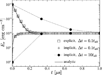
Figure 1.— Thermal evolution of radiation energy $E_{r}$. Crosses and squares denote results of explicit and implicit schemes, while solid curves do analytical solutions. The filled circles with dotted curves show the results of the implicit scheme with the time step of $\Delta t=10t_{ab}$.

4. Test Problems

In this section, we show results of some numerical tests for our RRHD code. This section consists of numerical tests for the radiation field (§ 4.1) and relativistic radiation hydrodynamics (§ 4.2). We assume that the closure relation is given by equation (61) so that the wave speed of radiation field is $1/\sqrt{3}$.

Figure 2.— Time evolution of $E_{r}$ (thick solid) and $F_{r}$ (solid). The optical depth of the system size is $0.01$. Dashed curves denote the light head $l_{c}=ct/\sqrt{3}$ at $t=0.5,1.0,1.5\tau_{c}$, where $\tau_{c}=L/c$. Dotted curves show analytical solutions assuming steady state given in equation (68).   Figure 3.— Time evolution of $E_{r}$ (thick solid) and $F_{r}$ (solid). The optical depth of the system size is unity. Dashed curves denote the light head $l_{c}=ct/\sqrt{3}$ at $t=0.5,1.0,1.5\tau_{c}$, where $\tau_{c}=L/c$. Dotted curves show analytical solutions assuming steady state given in equation (68).

Figure 4.— Snapshot of $E_{r}$ at $t=1.5\tau_{c}$. The solid, dashed and dotted curves denote contours at $10\%,0.1\%,10^{-3}\%$ of its maximum.   Figure 5.— Spatial profiles of $E_{r}$ at $t=1.5\tau_{c}$. Asterisks, squares, and filled circles indicate results along $y=0$, $x=0$, and $y=x$, respectively.

4.1. Numerical tests for Radiation Field

In this section, we show results of numerical tests for solving radiation fields given in equations (3). We assume that the fluid is static and uniform for simplicity. We recover the light speed as $c$ in this subsection. Equations are solved with 2nd order accuracy in space.

4.1.1 Radiative heating and cooling

This test has been proposed by Turner & Stone (2001). We evaluate the validity for the integration of the source term appeared in equation (20), which is implicitly and iteratively integrated in our numerical scheme. For this purpose, we start from a static and 1 zone fluid (i.e., number of grid points $N_{x}=1$), which is initially not in the thermal equilibrium with the radiation. From these assumptions, the radiation field obeys the following equation

$$\frac{dE_{r}}{dt}=\rho\kappa\left(4\pi\mathrm{B}-cE_{r}\right),$$ (66)

which is analytically integrated by assuming $\rho,\kappa$ and $\mathrm{B}$ are constant, and we obtain

$$E_{r}(t)=\frac{4\pi}{c}\mathrm{B}-\left(\frac{4\pi}{c}\mathrm{B}-E_{0}\right)e^{-\rho\kappa ct},$$ (67)

where $E_{0}$ is the radiation energy density at $t=0$. The radiation field approaches that in the Local Thermal Equilibrium (LTE, $E_{r}=4\pi\mathrm{B}/c$).

The mass density is set to $\rho=0.025~{}\mathrm{g~{}cm^{-3}}$ and the opacity is $\kappa=0.04~{}\mathrm{cm^{2}~{}g^{-1}}$, so that the corresponding absorption time scale is $t_{ab}\equiv 1/(\rho\kappa c)=3.3\times 10^{-8}~{}\mathrm{s}$. We examine two models of the initial radiation energy density, $E_{r}=10^{2}E_{\mathrm{LTE}}$ and $10^{-2}E_{\mathrm{LTE}}$, where $E_{\mathrm{LTE}}\equiv a_{R}T^{4}=10^{10}~{}\mathrm{erg~{}cm^{-3}}$. The specific heat ratio and the mean molecular weight are $\Gamma=5/3$ and $\mu=1.0$.

Table 1List of Simulation Runs

model	$\kappa$	$\Gamma$	state	$\rho$	$p_{g}$	$u^{x}$	$u^{y}$	$u^{z}$	$E_{r}^{\prime}$
RHDST1	0.4	$\frac{5}{3}$	L	1.0	$3.0\times 10^{-5}$	0.015	0	0	$1.0\times 10^{-8}$
			R	2.4	$1.61\times 10^{-4}$	$6.25\times 10^{-3}$	0	0	$2.50\times 10^{-7}$
RHDST2	0.2	$\frac{5}{3}$	L	1.0	$4.0\times 10^{-3}$	0.25	0	0	$2.0\times 10^{-5}$
			R	3.11	$0.04512$	$0.0804$	0	0	$3.46\times 10^{-3}$
RHDST3	0.3	2	L	1.0	60	10	0	0	2
			R	8	$2.34\times 10^{3}$	1.25	0	0	$1.13\times 10^{3}$
RHDST4	0.08	$\frac{5}{3}$	L	1.0	$6.0\times 10^{-3}$	0.69	0	0	0.18
			R	3.65	$3.59\times 10^{-2}$	0.189	0	0	$1.30$

Note. — Parameter sets of numerical tests. Scattering coefficient $\sigma_{s}$ is taken to be zero in all models.

Figure 1 shows the time evolution of $E_{r}$. Squares and crosses respectively denote results with explicit and implicit scheme for integrating the source term with the time step of $\Delta t=0.1t_{ab}$, while solid curves do analytical solutions obtained from equation (67). The data point for the model with $\Delta t=0.1t_{ab}$ is reduced for plotting. The lower and upper plots correspond to $E_{r}(t=0)=10^{-2}E_{\mathrm{LTE}}$ and $10^{2}E_{\mathrm{LTE}}$, respectively. We can see that results with both schemes excellently agree with analytical solutions when the time step is smaller than the absorption time scale $\Delta t<t_{ab}$. When $\Delta t=10t_{ab}$, solutions with implicit scheme (filled circle) stably reach the thermal equilibrium state, although they deviate from the analytical solutions before being in LTE. We note that the explicit scheme does not converge to the analytical solution when we take such a large time step. We also performed simulations with a much larger time step $\Delta t=10^{4}t_{ab}$ and found that solutions converge to analytical solution (not shown in figure). We also note that a number of iteration step used in the implicit scheme is less than or equal 2, even if $\Delta t=10^{4}t_{ab}$. Thus, the implicit scheme has a great advantage when the cooling timescale is much smaller than the dynamical timescale since we can take the numerical time step being $t_{ab}<\Delta t<t_{dyn}$. The computational time of explicit and implicit scheme with an equal number of time steps is $t_{\mathrm{exp}}:t_{\mathrm{imp}}=1:1.04$ with $\Delta t=0.1t_{ab}$.

4.1.2 Radiation transport

This test has been performed by Turner & Stone (2001). When the radiation is injected into uniform matter, it propagates with the characteristic wave velocity, while it exchanges energies with the plasma. As a test of this effect, we assume that the fluid is static and uniform in a simulation box bounded by $x=[0,L]$, where $L=1~{}\mathrm{cm}$. The radiation is injected from the boundary at $x=0$. In the uniform medium, the opacity is set to $\kappa=0.04~{}\mathrm{cm^{-2}~{}g}$. The radiation energy is $E_{\mathrm{LTE}}=10^{10}~{}\mathrm{erg~{}cm^{-3}}$ and the thermal energy is determined from the LTE condition. We examined two models of the mass density $\rho=0.25$ and $25~{}\mathrm{g~{}\mathrm{cm}^{-3}}$. The corresponding optical depth is $\tau=\rho\kappa L=0.01$ and $1$, respectively. At the boundary $x=0$, the radiation is injected with the energy density of $E_{r}=10^{10}E_{\mathrm{LTE}}$. The free boundary condition is applied at $x=L$. Other parameters are $\Gamma=5/3$, and $\mu=1.0$. The Courant-Friedrichs-Lewy (CFL) number is taken to be $0.5$.

Figure 3 shows results with $\tau=0.01$. Thick solid curves denote the radiation energy density, and thin solid curves show the radiation flux at $t=0.5,1.0,1.5\tau_{c}$ from left to right, where $\tau_{c}=L/c$. Since the radiation energy is injected from $x=0$, the wave front propagates from left to right as time goes on. The dashed curves denote the position of the light head $l_{c}=ct/\sqrt{3}$. Since we assume the Eddington approximation on the closure relation, the wave front propagates with the velocity $c/\sqrt{3}$. We can see that the wave front is sharply captured in our simulation code. In FLD approximations, the radiation field evolves obeying the diffusion equation, so that the wave front has a smooth profile (see, Fig. 7 in Turner & Stone, 2001). In our code, although we apply the Eddington approximation, the 1st order moment equation is solved. Then equations of the radiation field have hyperbolic form, so that the wave front can be captured using the HLL scheme.

Figure 3 shows results of the model of larger density ($\tau=1$). The radiation propagates with the velocity $c/\sqrt{3}$. Behind the wave front, the radiation field becomes steady and its energy exponentially decreases with $x$ (equivalently, $\tau=\kappa\rho x$) due to the absorption. When we assume the steady state and the radiation energy is much larger than that in LTE (i.e., $E_{r}\gg 4\pi\mathrm{B}/c$), equation (3) can be solved and we obtain

$$E_{r}=E_{0}\exp(-\sqrt{3}\rho\kappa x),~{}F_{r}=\frac{cE_{0}}{\sqrt{3}}\exp(-\sqrt{3}\rho\kappa x),$$ (68)

(Mihalas & Mihalas, 1984). Dotted curves in Fig. 3 and 3 show solutions obtained from equation (68). We can see that numerical results excellently recover analytical ones.

Figure 6.— Profiles of $\rho$, $p_{g}$, $v^{x}$, $E^{\prime}_{r}$ and $F^{\prime x}_{r}$ from top to bottom at $t=5000$ for the model RHDST1. Dots and solid curves denote for numerical and semi-analytical solutions.   Figure 7.— Profiles of $\rho$, $p_{g}$, $v^{x}$, $E^{\prime}_{r}$ and $F^{\prime x}_{r}$ from top to bottom at $t=5000$ for the model RHDST2. Dots and solid curves denote for numerical and semi-analytical solutions.

4.1.3 Radiation transport in 2-dimension

This test has been shown in Turner & Stone (2001) that the radiation field propagates in optically thin media in $x-y$ plane. The simulation domain is $x=[-L,L]$ and $y=[-L,L]$, where $L=1\mathrm{cm}$. Numerical grid points are $(N_{x},N_{y})=(400,400)$. The mass density of uniform fluid is $\rho=0.25~{}\mathrm{g~{}cm^{-3}}$. The other quantities are the same as those in § 4.1.2. At the initial state, a larger radiation energy is given inside $r=\sqrt{x^{2}+y^{2}}<0.1\mathrm{~{}cm}$ and its energy is $E_{r}=10^{10}E_{\mathrm{LTE}}$. The free (Neumann) boundary condition is applied on each side of the box. The CFL condition is taken as $0.5$.

Figure 5 shows contours of radiation energy density $E_{r}$ at $t=1.5\tau_{c}$. The solid, dashed, and dotted curves denote contours at $10\%,0.1\%,10^{-3}\%$ of its maximum. Due to the enhancement of radiation energy around the origin at the initial state, the radiation field propagates in a circle, forming a caldera-shaped profile of the radiation energy density. The wave front propagates with the speed of $c/\sqrt{3}$. Figure 5 shows one dimensional cut of results at $t=1.5\tau_{c}$. Asterisks, squares and filled circles show results along $y=0$, $x=0$, and $y=x$, respectively. We can see that the wave packet has a sharp structure. The radiation energy is mainly accumulated around the wave front, while it is very small inside the wave front (caldera floor). Such the caldera structure is not successfully reproduced when we apply FLD approximation (Turner & Stone, 2001) since the FLD is formulated based on the diffusion approximation. Although the wave speed reduces to $c/\sqrt{3}$, solving the 1st order moment in radiation field (radiation flux) with Eddington approximation has an advantage for studying the propagation of the radiation pulse in optically thin media.

In the problem of $\S~{}\ref{radtransport}$ and $\S~{}\ref{radtransport2}$, the radiation field passes the boundary $x=L$ at $t=\sqrt{3}\tau_{c}$. When we adopt the free (Neumann) boundary conditions, most of the radiation energy passes the boundary, while some part of it is reflected and stays in the simulation box. An amplitude of the reflected wave $E_{\mathrm{ref}}$ is smaller than that passing the boundary $E_{\mathrm{pass}}$, $\max[E_{\mathrm{ref}}/E_{\mathrm{pass}}]\sim 0.8\%$ for the one-dimensional test and $\sim 5\%$ for the two dimensional test. The waves are mainly reflected at the corner of the simulation box in the two dimensional simulation (i.e., around $[x,y]=[\pm L,\pm L]$). The simple free boundary condition can be applied in the radiation field with this accuracy.

Figure 8.— Profiles of $\rho$, $p_{g}$, $v^{x}$, $E^{\prime}_{r}$ and $F^{\prime x}_{r}$ from top to bottom at $t=5000$ for the model RHDST3. Dots and solid curves denote for numerical and semi-analytical solutions.   Figure 9.— $L$-1 norms of $\rho$, $p_{g}$, $u^{x}$, $E^{\prime}_{r}$ and $F^{\prime x}_{r}$ for the model RHDST3.

4.2. Numerical Test for Relativistic Radiation Hydrodynamics

Next, we consider the coupling between the radiation and matter fields. We solve RRHD equations with a second order accurate scheme.

Test problems for radiative shock shown in this subsection are developed by Farris et al. (2008) who proposed and solved four shock tube test problems. Initial conditions of these problems are listed in Table 1. The initial state has a discontinuity at $x=0$ and the system is in LTE. Such an initial discontinuity breaks up generating waves. When the waves pass away from the simulation box, the system approaches the steady state. Then we compare our numerical results with semi-analytical solutions after the system reaches a steady state. In Farris et al. (2008), the initial condition is constructed by boosting semi-analytical solutions, so that the shock moves with an appropriate velocity. In our test, the shock is assumed to rest around $x=0$ (shock rest frame). Such the problem can be more stringent tests for our code to maintain the stationarity (Zanotti et al., 2011).

The simulation box is bounded by $x=[-L,L]$, where $L=20$ in the normalized unit, and a number of numerical grid points is $N_{x}=3200$. The free boundary condition is applied at $x=\pm L$. We give the physical quantities at the left and right state of $\rho,p,u,E_{r}^{\prime}$ and flux is assumed to be zero. Following Farris et al. (2008), the Stefan-Boltzmann constant is normalized such that $4\pi a_{R}=E^{\prime}_{r,L}/T_{L}^{4}=E^{\prime}_{r,R}/T_{R}^{4}$, where the subscripts $L$ and $R$ denote the quantities at the left ($x\leq 0$) and right ($x>0$).

We note that although we adopt an iteration method to integrate stiff source term (equation (38)), solutions in the following tests converge within the relative error of $10^{-6}$ without iterations.

Figure 10.— Profiles of $\rho$, $p_{g}$, $v^{x}$, $E^{\prime}_{r}$ and $F^{\prime x}_{r}$ from top to bottom at $t=5000$ for the model RHDST4. Dots and solid curves denote for numerical and semi-analytical solutions.   Figure 11.— $L$-1 norms of $\rho$, $p_{g}$, $u^{x}$, $E^{\prime}_{r}$ and $F^{\prime x}_{r}$ for the model RHDST4.

4.2.1 Non-relativistic shock

In this test, the non-relativistic strong shock exists at $x=0$ (model RHDST1). The ratio of the radiation to thermal energy in the upstream ($x<0$) is $2.2\times 10^{-4}$. We take the CFL condition to be $0.9$. Fig. 7 shows profile at $t=5000$. The physical quantities shown in this figure are $\rho$, $p_{g}$, $v^{x}$, $E_{r}^{\prime},F^{\prime x}_{r}$ from top to bottom. (We note that $F^{\prime x}_{r}$, which is the radiation flux measured in the comoving frame, is different from $F^{x}$ defined in Farris et al. 2008 by factor $\gamma$). Dots and curves denote for the numerical and semi-analytical solutions.

Since we give an initial condition by a step function at $x=0$, waves arisen at the discontinuity propagate in the $\pm x-$direction (mainly in the $+x$-direction since the upstream is supersonic). After the waves pass the boundary at $x=\pm L$, the system reaches the steady state.

Since the radiation energy is negligible, fluid quantities have jumps around $x=0$ similar to pure hydrodynamical shock. The radiation field, on the other hand, has a smooth profile in which the radiation energy is transported in front of the shock. The radiation energy and flux have no discontinuities. The simulation results are well consistent with analytical solutions.

4.2.2 Mildly relativistic shock

In this test, the mildly-relativistic strong shock exists at $x=0$ (model RHDST2). The ratio of the radiation to thermal energy in the upstream is $3.3\times 10^{-3}$. We take the CFL condition to be $0.9$. Fig. 7 shows profiles at $t=5000$. The physical quantities shown in this figure are $\rho$, $p_{g}$, $v^{x}$, $E_{r}^{\prime},F^{\prime x}_{r}$ from top to bottom. We can see that the radiation energy density is no more continuous but jumps at $x=0$. In the non-relativistic limit, the radiation energy density and its flux are continuous, but it is not the case in general. They are no more the conserved variables at the shock in the relativistic flow (Farris et al., 2008). The solutions obtained in our numerical simulation (dots) are qualitatively and quantitatively consistent with semi-analytical solutions (solid curves).

4.2.3 Relativistic shock

In this test, the highly-relativistic strong shock exists at $x\simeq 0$ (model RHDST3). The upstream Lorentz factor is $\sim 10$ and the ratio of the radiation to thermal energy is $3.3\times 10^{-2}$. We take the CFL condition to be $0.9$. Fig. 9 shows profile at $t=5000$. The physical quantities shown in this figure are $\rho$, $p_{g}$, $v^{x}$, $E_{r}^{\prime},F^{\prime x}_{r}$ from top to bottom.

After waves generated at the jump $(x=0)$ passes the boundary, the system approaches the steady state. In this case, all the physical quantities are continuous.

The solutions obtained in our numerical simulation excellently recover analytical solutions even when the flow speed is highly relativistic. To validate our numerical code, we compute the $L$-1 norms from

$$L_{1}[f]=\Delta x\sum_{i=1}{N_{x}}|f_{i}-f_{\mathrm{a}}(x_{i})|,$$ (69)

where $f_{i}$ is the physical quantity at the $i$-th grid and $f_{\mathrm{a}}$ is the semi-analytic solution.

We perform simulations with number of grid points $N_{x}=400,800,1600,3200$. In these tests, we use the semi-analytic solution as the initial condition. Figure 9 shows the $L$-1 norms of errors in $\rho,u^{x},p_{g},E_{r}^{\prime}$, and $F^{\prime x}_{r}$. We can see that all errors converges at second order in $\Delta x$.

4.2.4 Radiation dominated shock

In this test, the mildly-relativistic, radiation dominated shock exists at $x\simeq 0$ (model RHDST4). The ratio of the radiation to thermal energy in the upstream is $20$. We take the CFL condition to be $0.3$. Fig. 11 shows profile at $t=5000$. The physical quantities shown in this figure are $\rho$, $p_{g}$, $v^{x}$, $E_{r}^{\prime},F^{\prime x}_{r}$ from top to bottom.

After waves generated at the jump $(x=0)$ pass the boundary, the system approaches the steady state. In this case, all the physical quantities are continuous and their profiles are very smooth since a precursor generated from the shock strongly affects the plasma.

We again find very good agreement with semi-analytical solutions even when the radiation energy dominates the thermal energy. Figure 11 shows the $L$-1 norms of errors in $\rho,u^{x},p_{g},E_{r}^{\prime}$, and $F^{\prime x}_{r}$. In this test, we adopt the analytical solution as an initial condition following Farris et al. (2008). We can see that all errors converges at second order in $\Delta x$.

5. Discussion

In the current study, we construct the relativistic hydrodynamic simulation code including the radiation field. The magnetic field, which would play a crucial role in the relativistic phenomena, is neglected for simplicity. It would be quiet simple to include the magnetic field using a well-developed numerical scheme. When we extend our radiation hydrodynamic code to the radiation magnetohydrodynamic one, the energy momentum tensor $T_{\mathrm{HD}}^{\nu,\mu}$ is replaced by that of the magnetofluids,

$$T^{\mu\nu}_{\mathrm{MHD}}=(\rho\xi+b^{2})u^{\mu}u^{\nu}-b^{\mu}b^{\nu}+\left(p_{g}+\frac{b^{2}}{2}\right)\eta^{\mu\nu},$$ (70)

where $b^{\nu}=\left\{\mbox{\boldmath$u$}\cdot\mbox{\boldmath$B$},\left[\mbox{\boldmath$B$}+(\mbox{\boldmath$u$}\cdot\mbox{\boldmath$B$})\mbox{\boldmath$u$}\right]/\gamma\right\}$ is the covariant form of the magnetic fields. The magnetic field evolves according to the induction equation for the ideal MHD,

$$\partial_{\nu}(u^{\nu}b^{\mu}-u^{\mu}b^{\nu})=0.$$ (71)

Then the energy momentum conservation equation and the induction equation are explicitly integrated using the HLL or higher order approximate Riemann solvers (Mignone & Bodo, 2005, 2006; Honkkila & Janhunen, 2007; Mignone et al., 2009). The source term describing the interaction between the matter and the radiation, is integrated by applying our proposed scheme.

Another simplification made in this paper is adopting the Eddington approximation that the radiation field is assumed to be isotropic in the comoving frame. The wave velocity of radiation field has a propagation speed of $c/\sqrt{3}$. This would become an issue when the flow speed is relativistic ($v\simeq c$). The flow speed, in principle, exceeds the phase speed of light mode so that the radiation energy might accumulate in front of the plasma flow. Also the problem appears when we consider the magnetofluids. The fast magnetosonic wave speed can exceeds the reduced light speed $c/\sqrt{3}$. Another problem is that the radiation does not propagate in a straight line since we assume that the radiation field is isotropic. When the optically thick medium with a finite volume is irradiated from one side, there should be a shadow on the other side (Hayes & Norman, 2003). Such a shadow is no longer formed when we utilize the Eddington approximation (González et al., 2007). To overcome these problems, we should admit an anisotropy of radiation flux in a comoving frame (Kershaw, 1976; Minerbo, 1978; Levermore, 1984). In our formulation, we do not specify the closure relation until § 3.3. Thus we can employ M-1 closure by replacing matrix $A(u)$ without the other modification. The explicit-implicit scheme of the relativistic radiation magnetohydrodynamics with the M-1 closure will be reported in the near future.

6. Summary

We have developed a numerical scheme for solving special relativistic radiation hydrodynamics, which ensures the conservation of total energy and flux. The hyperbolic term is explicitly solved using an approximate Riemann solver, while the source term describing the interaction between the matter and the radiation, is implicitly integrated using an iteration method. The advantage of the implicit scheme is that we can take the numerical time step larger than the absorption and scattering time scale. This allows us to study the long term evolution of the system (typically, the dynamical timescale).

When integrating the source term, we need to invert matrices $C$ and $A$ in our proposed scheme. We have to note that the rank of these matrices used in the implicit scheme is very small ($4\times 4$ for $C$ and $6\times 6$ for $A$). This is because the interaction between the radiation and the gas is described by a local nature (source term) when we solve 0th and 1st moments for radiation. This means that the numerical code can be easily parallelized and a high parallelization efficiency is expected.

We note that since the matrix $C$ is only $4\times 4$ matrix, we can invert it analytically. For the matrix $A$, it is relatively small matrix but it is difficult to invert it analytically. Thus we decide to use LU decomposition method. Since the LU decomposition method can invert the matrix directly without iterations, we obtain $\mbox{\boldmath$A$}^{-1}$ stably.

We find that the wave front of radiation field can be sharply captured using the HLL scheme even when we adopt the simple closure relation $P^{\prime ij}_{r}=\delta^{ij}/3$ (i.e., the Eddington approximation). When we adopt the FLD approximations, such a sharp wave front cannot be captured due to the diffusion approximations. Thus, solving the 1st order moment of radiation has an advantage when we consider the optically thin medium although the wave speed reduces to $c/\sqrt{3}$ and the radiation field is isotropic.

We adopted the iteration scheme to integrate stiff source terms. If we need many counts in iteration scheme, it causes a load imbalance between each core when the code is parallelized. But we have to stress that solutions converged only within two steps even if $\Delta t=10^{4}t_{ab}$ for the problem of radiative heating and cooling appeared in § 4.1.1. For the other tests, solution converges without iteration. Thus we can expect that the load imbalance due to the iteration scheme is not severe even in the more realistic problems.

In the previous papers (Farris et al., 2008; Zanotti et al., 2011), radiation fields are defined in different frames for primitive and conservative variables (mixed frame). In such a method, the radiation moment equations are simply described. However, this method is not suitable for implicit integration. This is because that a Lorentz transformation between two frames is needed. By the transformation, expressions of the radiation fields become quite complex even if the Eddington approximation is adopted. Moreover, the radiation stress tensor, Pr, is generally non-liner function of the radiation energy density and the radiation flux through the Eddington tensor. Thus, extension of explicit method to implicit method is not straightforward for the relativistic radiation hydrodynamics.

In our method, we treat radiation fields in the laboratory frame, only. Such a treatment simplifies implicit integration. Although we need to invert $6\times 6$ matrix and $4\times 4$ matrix, our new method is easier than the method with mixed frame. Two matrices of $C$ (which is needed for implicit integration) and $A$ (which is needed to compute Pr) are directly inverted using analytical solution and LU-decomposition method. Since we need not to use some iteration methods to invert them, our method is stable and comparatively easy. Our method would be quite useful for numerical simulations of relativistic astrophysical phenomena, e.g., black hole accretion disks, relativistic jets, gamma-ray bursts, end so on, since both the high density region and high velocity region exists, and since the radiation processes are play important role for dynamics as well as energetics.

Appendix A calculating $P_{r}^{ij}$

In this appendix, we show how to obtain the radiation stress in the observer frame from $E_{r}$ and $F_{r}^{i}$ by assuming the Eddington approximation. $P_{r}^{ij}$ is the $3\times 3$ symmetric matrix and there are six unknowns. Since equation (62) is a linear with $E_{r}$ and $F_{r}^{i}$, we need to solve 6th order linear equations,

$$\mbox{\boldmath$A$}p=r,$$ (A1)

where $\mbox{\boldmath$A$}=\{a_{ij}\}$, $p^{T}=(P_{r}^{11},P_{r}^{22},P_{r}^{33},P_{r}^{12},P_{r}^{13},P_{r}^{23})$, and $r^{T}=(R^{11},R^{22},R^{33},R^{12},R^{13},R^{23})$. The explicit form of $a_{ij}$ is written as

$$a_{11} = 1+(u_{1})(u_{1})\left[-\frac{1}{3}+\frac{(u^{1})^{2}}{(1+\gamma)^{2}}\right]+\frac{2u^{1}u_{1}}{1+\gamma},$$ (A2)

$$a_{12} = (u_{2})(u_{2})\left[-\frac{1}{3}+\frac{(u^{1})^{2}}{(1+\gamma)^{2}}\right],$$ (A3)

$$a_{13} = (u_{3})(u_{3})\left[-\frac{1}{3}+\frac{(u^{1})^{2}}{(1+\gamma)^{2}}\right],$$ (A4)

$$a_{14} = (u_{1})(u_{2})\left[-\frac{1}{3}+\frac{(u^{1})^{2}}{(1+\gamma)^{2}}\right]+\frac{2u^{1}u_{2}}{1+\gamma},$$ (A5)

$$a_{15} = (u_{1})(u_{3})\left[-\frac{1}{3}+\frac{(u^{1})^{2}}{(1+\gamma)^{2}}\right]+\frac{2u^{1}u_{3}}{1+\gamma},$$ (A6)

$$a_{16} = (u_{2})(u_{3})\left[-\frac{1}{3}+\frac{(u^{1})^{2}}{(1+\gamma)^{2}}\right]$$ (A7)

$$a_{21} = (u_{1})(u_{1})\left[-\frac{1}{3}+\frac{(u^{2})^{2}}{(1+\gamma)^{2}}\right],$$ (A8)

$$a_{22} = 1+(u_{2})(u_{2})\left[-\frac{1}{3}+\frac{(u^{2})^{2}}{(1+\gamma)^{2}}\right]+\frac{2u^{2}u_{2}}{1+\gamma},$$ (A9)

$$a_{23} = (u_{3})(u_{3})\left[-\frac{1}{3}+\frac{(u^{2})^{2}}{(1+\gamma)^{2}}\right],$$ (A10)

$$a_{24} = (u_{1})(u_{2})\left[-\frac{1}{3}+\frac{(u^{2})^{2}}{(1+\gamma)^{2}}\right]+\frac{2u^{2}u_{1}}{1+\gamma},$$ (A11)

$$a_{25} = (u_{1})(u_{3})\left[-\frac{1}{3}+\frac{(u^{2})^{2}}{(1+\gamma)^{2}}\right],$$ (A12)

$$a_{26} = (u_{2})(u_{3})\left[-\frac{1}{3}+\frac{(u^{2})^{2}}{(1+\gamma)^{2}}\right]+\frac{2u^{2}u_{3}}{1+\gamma},$$ (A13)

$$a_{31} = (u_{1})(u_{1})\left[-\frac{1}{3}+\frac{(u^{3})^{2}}{(1+\gamma)^{2}}\right],$$ (A15)

$$a_{32} = (u_{2})(u_{2})\left[-\frac{1}{3}+\frac{(u^{3})^{2}}{(1+\gamma)^{2}}\right],$$ (A16)

$$a_{33} = 1+(u_{3})(u_{3})\left[-\frac{1}{3}+\frac{(u^{3})^{2}}{(1+\gamma)^{2}}\right]+\frac{2u^{3}u_{3}}{1+\gamma},$$ (A17)

$$a_{34} = (u_{1})(u_{2})\left[-\frac{1}{3}+\frac{(u^{3})^{2}}{(1+\gamma)^{2}}\right],$$ (A18)

$$a_{35} = (u_{1})(u_{3})\left[-\frac{1}{3}+\frac{(u^{3})^{2}}{(1+\gamma)^{2}}\right]+\frac{2u^{3}u_{1}}{1+\gamma},$$ (A19)

$$a_{36} = (u_{2})(u_{3})\left[-\frac{1}{3}+\frac{(u^{3})^{2}}{(1+\gamma)^{2}}\right]+\frac{2u^{3}u_{2}}{1+\gamma},$$ (A20)

$$a_{41} = \frac{(u^{1})(u^{2})(u_{1})(u_{1})}{(1+\gamma)^{2}}+\frac{(u^{2})(u_{1})}{1+\gamma},$$ (A21)

$$a_{42} = \frac{(u^{1})(u^{2})(u_{2})(u_{2})}{(1+\gamma)^{2}}+\frac{(u^{1})(u_{2})}{1+\gamma},$$ (A22)

$$a_{43} = \frac{(u^{1})(u^{2})(u_{3})(u_{3})}{(1+\gamma)^{2}},$$ (A23)

$$a_{44} = 1+\frac{(u^{1})(u^{2})(u_{1})(u_{2})}{(1+\gamma)^{2}}+\frac{(u^{1})(u_{1})+(u^{2})(u_{2})}{1+\gamma},$$ (A24)

$$a_{45} = \frac{(u^{1})(u^{2})(u_{1})(u_{3})}{(1+\gamma)^{2}}+\frac{(u^{2})(u_{3})}{1+\gamma},$$ (A25)

$$a_{46} = \frac{(u^{1})(u^{2})(u_{2})(u_{3})}{(1+\gamma)^{2}}+\frac{(u^{1})(u_{3})}{1+\gamma},$$ (A26)

$$a_{51} = \frac{(u^{1})(u^{3})(u_{1})(u_{1})}{(1+\gamma)^{2}}+\frac{(u^{3})(u_{1})}{1+\gamma},$$ (A28)

$$a_{52} = \frac{(u^{1})(u^{3})(u_{2})(u_{2})}{(1+\gamma)^{2}},$$ (A29)

$$a_{53} = \frac{(u^{1})(u^{3})(u_{3})(u_{3})}{(1+\gamma)^{2}}+\frac{(u^{1})(u_{3})}{1+\gamma},$$ (A30)

$$a_{54} = \frac{(u^{1})(u^{3})(u_{1})(u_{2})}{(1+\gamma)^{2}}+\frac{(u^{3})(u_{2})}{1+\gamma},$$ (A31)

$$a_{55} = 1+\frac{(u^{1})(u^{3})(u_{1})(u_{3})}{(1+\gamma)^{2}}+\frac{(u^{1})(u_{1})+(u^{3})(u_{3})}{1+\gamma},$$ (A32)

$$a_{56} = \frac{(u^{1})(u^{3})(u_{2})(u_{3})}{(1+\gamma)^{2}}+\frac{(u^{1})(u_{2})}{1+\gamma},$$ (A33)

$$a_{61} = \frac{(u^{2})(u^{3})(u_{1})(u_{1})}{(1+\gamma)^{2}},$$ (A35)

$$a_{62} = \frac{(u^{2})(u^{3})(u_{2})(u_{2})}{(1+\gamma)^{2}}+\frac{(u^{3})(u_{2})}{1+\gamma},$$ (A36)

$$a_{63} = \frac{(u^{2})(u^{3})(u_{3})(u_{3})}{(1+\gamma)^{2}}+\frac{(u^{2})(u_{3})}{1+\gamma},$$ (A37)

$$a_{64} = \frac{(u^{2})(u^{3})(u_{1})(u_{2})}{(1+\gamma)^{2}}+\frac{(u^{3})(u_{1})}{1+\gamma},$$ (A38)

$$a_{65} = \frac{(u^{2})(u^{3})(u_{1})(u_{3})}{(1+\gamma)^{2}}+\frac{(u^{2})(u_{1})}{1+\gamma},$$ (A39)

$$a_{66} = 1+\frac{(u^{2})(u^{3})(u_{2})(u_{3})}{(1+\gamma)^{2}}+\frac{(u^{2})(u_{2})+(u^{3})(u_{3})}{1+\gamma}.$$ (A40)

In our numerical code, the matrix $A$ is inverted using $LU$-decomposition method.

Also $(\partial P^{ij})/(\partial E_{r})$ and $(\partial P^{ij})/(\partial F_{r}^{k})$ are obtained by solving the following equations

$$A\frac{\partial p}{\partial E_{r}}=\frac{\partial r}{\partial E_{r}},~{}A\frac{\partial p}{\partial F^{k}_{r}}=\frac{\partial r}{\partial F^{k}_{r}},$$ (A41)

where,

$$\frac{\partial R^{ij}}{\partial E_{r}} = \frac{\gamma^{2}}{3}\delta^{ij}-u^{i}u^{j},$$ (A42)

$$\frac{\partial R^{ij}}{\partial F_{r}^{k}} = -\frac{2}{3}\gamma\delta^{ij}u^{k}+u^{i}\delta^{j}_{k}+u^{j}\delta^{i}_{k}+\frac{2}{1+\gamma}u^{i}u^{j}u_{k}.$$ (A43)

Since the matrix $A$ is a function of $u$ and independent of $E_{r}$ and $F^{k}_{r}$, matrix $A^{-1}$ is computed once before calculating $P^{ij}_{r},(\partial P^{ij}_{r})/(\partial E_{r})$ and $(\partial P_{r}^{ij})/(\partial F_{r}^{k})$.

References

- Balbus & Hawley (1991) Balbus, S. A. & Hawley, J. F. 1991, ApJ, 376, 214
- Bisnovatyi-Kogan & Blinnikov (1977) Bisnovatyi-Kogan, G. S. & Blinnikov, S. I. 1977, A&A, 59, 111
- Blandford & Payne (1982) Blandford, R. D. & Payne, D. G. 1982, MNRAS, 199, 883
- Blandford & Znajek (1977) Blandford, R. D. & Znajek, R. L. 1977, MNRAS, 179, 433
- Colella & Woodward (1984) Colella, P. & Woodward, P. R. 1984, Journal of Computational Physics, 54, 174
- Farris et al. (2008) Farris, B. D., Li, T. K., Liu, Y. T., & Shapiro, S. L. 2008, Phys. Rev. D, 78, 024023
- González et al. (2007) González, M., Audit, E., & Huynh, P. 2007, A&A, 464, 429
- Harten et al. (1983) Harten, A., Lax, P. D., & van Leer, B. 1983, SIAM Rev., 25, 35
- Hawley et al. (1995) Hawley, J. F., Gammie, C. F., & Balbus, S. A. 1995, ApJ, 440, 742
- Hayashi et al. (1996) Hayashi, M. R., Shibata, K., & Matsumoto, R. 1996, ApJ, 468, L37+
- Hayes & Norman (2003) Hayes, J. C. & Norman, M. L. 2003, ApJS, 147, 197
- Hirose et al. (2009) Hirose, S., Blaes, O., & Krolik, J. H. 2009, ApJ, 704, 781
- Honkkila & Janhunen (2007) Honkkila, V. & Janhunen, P. 2007, Journal of Computational Physics, 223, 643
- Kato et al. (2008) Kato, S., Fukue, J., & Mineshige, S. 2008, Black-Hole Accretion Disks — Towards a New Paradigm —, ed. Kato, S., Fukue, J., & Mineshige, S.
- Kato et al. (2004) Kato, Y., Hayashi, M. R., & Matsumoto, R. 2004, ApJ, 600, 338
- Kershaw (1976) Kershaw, D. S. 1976, Lawrence Livermore National Laboratory, UCRL
- Koide et al. (2002) Koide, S., Shibata, K., Kudoh, T., & Meier, D. L. 2002, Science, 295, 1688
- Komissarov (1999) Komissarov, S. S. 1999, MNRAS, 308, 1069
- Levermore (1984) Levermore, C. D. 1984, J. Quant. Spec. Radiat. Transf., 31, 149
- Lightman & Eardley (1974) Lightman, A. P. & Eardley, D. M. 1974, ApJ, 187, L1+
- Lovelace (1976) Lovelace, R. V. E. 1976, Nature, 262, 649
- Martí & Mueller (1996) Martí, J. & Mueller, E. 1996, Journal of Computational Physics, 123, 1
- McKinney & Blandford (2009) McKinney, J. C. & Blandford, R. D. 2009, MNRAS, 394, L126
- Meier et al. (2001) Meier, D. L., Koide, S., & Uchida, Y. 2001, Science, 291, 84
- Mignone & Bodo (2005) Mignone, A. & Bodo, G. 2005, MNRAS, 364, 126
- Mignone & Bodo (2006) —. 2006, MNRAS, 368, 1040
- Mignone et al. (2009) Mignone, A., Ugliano, M., & Bodo, G. 2009, MNRAS, 393, 1141
- Mihalas & Mihalas (1984) Mihalas, D. & Mihalas, B. W. 1984, Foundations of radiation hydrodynamics (New York, Oxford University Press, 1984, 731 p.)
- Minerbo (1978) Minerbo, G. N. 1978, J. Quant. Spec. Radiat. Transf., 20, 541
- Nunohiro & Hirano (2003) Nunohiro, E. & Hirano, S. 2003, Trans. Japan Soc. Ind. Appl. Math., 13, 159
- Ohsuga (2006) Ohsuga, K. 2006, ApJ, 640, 923
- Ohsuga & Mineshige (2011) Ohsuga, K. & Mineshige, S. 2011, ApJ, 736, 2
- Ohsuga et al. (2009) Ohsuga, K., Mineshige, S., Mori, M., & Kato, Y. 2009, PASJ, 61, L7+
- Ohsuga et al. (2005) Ohsuga, K., Mori, M., Nakamoto, T., & Mineshige, S. 2005, ApJ, 628, 368
- Okuda et al. (2009) Okuda, T., Lipunova, G. V., & Molteni, D. 2009, MNRAS, 398, 1668
- Palenzuela et al. (2009) Palenzuela, C., Lehner, L., Reula, O., & Rezzolla, L. 2009, MNRAS, 394, 1727
- Sekora & Stone (2009) Sekora, M. & Stone, J. 2009, Communications in Applied Mathematics and Computational Science, 4, 135
- Shakura & Sunyaev (1976) Shakura, N. I. & Sunyaev, R. A. 1976, MNRAS, 175, 613
- Shibata et al. (2011) Shibata, M., Kiuchi, K., Sekiguchi, Y., & Suwa, Y. 2011, Progress of Theoretical Physics, 125, 1255
- Shibazaki & Hōshi (1975) Shibazaki, N. & Hōshi, R. 1975, Progress of Theoretical Physics, 54, 706
- Sikora et al. (1996) Sikora, M., Sol, H., Begelman, M. C., & Madejski, G. M. 1996, MNRAS, 280, 781
- Stone et al. (1992) Stone, J. M., Mihalas, D., & Norman, M. L. 1992, ApJS, 80, 819
- Takahashi & Masada (2011) Takahashi, H. R. & Masada, Y. 2011, ApJ, 727, 106
- Takeuchi et al. (2010) Takeuchi, S., Ohsuga, K., & Mineshige, S. 2010, PASJ, 62, L43+
- Turner & Stone (2001) Turner, N. J. & Stone, J. M. 2001, ApJS, 135, 95
- Uchida & Shibata (1985) Uchida, Y. & Shibata, K. 1985, PASJ, 37, 515
- van Leer (1977) van Leer, B. 1977, Journal of Computational Physics, 23, 263
- Zanotti et al. (2011) Zanotti, O., Roedig, C., Rezzolla, L., & Del Zanna, L. 2011, MNRAS, 1386
- Zenitani et al. (2009) Zenitani, S., Hesse, M., & Klimas, A. 2009, ApJ, 696, 1385