Quantum phase transition in a three-level atom-molecule system

Abstract

We adopt a three-level bosonic model to investigate the quantum phase transition in an ultracold atom-molecule conversion system which includes one atomic mode and two molecular modes. Through thoroughly exploring the properties of energy level structure, fidelity, and adiabatical geometric phase, we confirm that the system exists a second-order phase transition from an atom-molecule mixture phase to a pure molecule phase. We give the explicit expression of the critical point and obtain two scaling laws to characterize this transition. In particular we find that both the critical exponents and the behaviors of ground-state geometric phase change obviously in contrast to a similar two-level model. Our analytical calculations show that the ground-state geometric phase jumps from zero to $\pi/3$ at the critical point. This discontinuous behavior has been checked by numerical simulations and it can be used to identify the phase transition in the system.

I Introduction

Quantum phase transition (QPT) is one of the most important concepts in the many-body quantum theory. As a central fundamental transition phenomenon at the temperature of absolute zero, it describes an abrupt change in the ground state of a many-body system due to its quantum fluctuations sachdevs2003 ; sondhisl1997 . The experimental observation of a QPT from a superfluid (SF) to a Mott insulator (MI) in a gas of ultracold atoms greinerm2002 inspired great interest in investigating clean, highly controllable, and strong correlated bosonic systems tilahund2011 . Actually, the ultracold atomic gases pitaevskiil2003 have become an ideal platform to study many-body physics because of their enormous applications and the advanced experimental techniques available in the fields of atomic and optical physics ruseckasj2005 .

In recent years, a remarkable development in the aforementioned filed is to convert ultracold atoms to molecules via Feshbach resonance Donleyea2002 ; xuk2003 ; Herbigj2003 or photoassociation Wynarr2000 ; Romt2004 ; whinklerk2005 techniques. Compared with the fermionic model in this kind of systems, the bosonic model is of interest for theoretically exploring the QPTs. When both ultracold atoms and molecules are bosons, the systems possess a few degrees of freedom and a large particle number which can greatly simplify the calculations. On the other hand, the atom-molecule conversion systems can be well described by a mean-field theory when the particle number is large enough and this treatment will lead to nonlinearity. These features have stimulated much efforts to study the adiabatic evolution Gaubatzu1988 ; Kuklinskijr1989 ; Pazye2005 ; linghy2007 ; Shapiroea2007 ; mengsy08 , geometric phase fulb2010 ; wub2011 , and phase transition santosg10 ; lisc11a of the systems. Instead of the traditional approaches for describing a QTP (i.e., using the concepts of order parameter and symmetry breaking), very recently Santos el al. adopted the concepts of entanglement and fidelity to investigate the QPT in a two-level bosonic atom-molecule system santosg10 . Motivated by this work we discussed same problems from the perspectives of scaling laws and Berry curvature lisc11a . However, the connection between the mean-field Berry phase and the phase transition in this type of bosonic model, and the properties of the QPT in a three-level atom-molecule system are still unresolved, which call for further theoretical considerations.

As a continuous work, in this paper we investigate the quantum phase transition in an ultracold atom-molecule conversion system by adopting a $\Lambda$-type three-level bosonic model. Based on this model, we first discuss the structure of quantum energy levels and analyze the properties of ground state. In order to compare the phase transition properties with a similar two-level model santosg10 , we study the energy gap, the ground-state fidelity, and mean-field geometric phase. We illustrate that, when the ratio of the coupling strength between two molecular modes to that between atomic mode and the upper molecular mode exceeds a critical value, a similar QPT from a mixed atom-molecule phase to a pure molecular phase is also observed in our system. To characterize this transition we obtain the analytical expression of the critical point by using the mean-field approach and derive two critical exponents via numerically studying scaling laws. In particular we calculate the ground-state geometric phase and find its discontinuous behavior at the phase transition point.

Our paper is organized as follow: In Sec. II we give the second-quantized model and its mean-field description. In Sec. III we explore the properties of energy levels and ground states. In Sec. IV we choose the characteristic scaling law, fidelity, and adiabatic geometric phase to describe the QPT. Section V presents our conclusion.

II Three-level model and mean-field description

The system we consider here is illustrated schematically in Fig. 1. It describes the process of creating ultracold diatomic molecules from bosonic condensed atoms, which constitutes a $\Lambda$-type three-level model. In the three-mode description, each mode $|\alpha\rangle$ ($\alpha=a,g$, and $e$ respectively represent the atomic mode, the ground-state molecular mode, and the excited-state molecular mode) is associated with an annihilation operator $\hat{\beta}$ ($\beta=a,b_{g}$, and $b_{e}$) due to the basic assumption that the spatial wavefunctions for these modes are fixed. By setting the energy of atomic mode as zero, the Hamiltonian of the system takes the following second-quantized form with $\hbar=1$ wub2011 :

$$\hat{H}_{S}= \omega_{e}\hat{b}_{e}^{\dagger}\hat{b}_{e}+\omega_{g}\hat{b}_{g}^{\dagger}\hat{b}_{g}+$$

$$\Omega_{d}e^{i\nu_{d}t}\hat{b}_{e}^{\dagger}\hat{b}_{g}+\frac{\Omega_{p}e^{-i\nu_{p}t}}{\sqrt{N}}\hat{b}_{e}^{\dagger}\hat{a}\hat{a}+\mathrm{H.c.},$$ (1)

where the abbreviation $\mathrm{H.c.}$ denotes the operation of Hermitian conjugate. $\nu_{d}$ and $\nu_{p}$ are the frequencies of two laser pulses $\Omega_{d}$ and $\Omega_{p}$, respectively. The frequencies $\omega_{g}$ and $\omega_{e}$ measure the molecular ground state and excited state energies, respectively. The total atom number $N=N_{a}+2(N_{g}+N_{e})$ with $N_{a}=\hat{a}^{\dagger}\hat{a}$, $N_{g}=\hat{b}_{g}^{\dagger}\hat{b}_{g}$, and $N_{e}=\hat{b}_{e}^{\dagger}\hat{b}_{e}$, commutes with the Hamiltonian (II) and is therefore conserved. Notice that the laser pulse parameter $\Omega_{p}$ can be complex. To achieve this one can split the laser pulse into two beams and then recombine and focus them on the system. As a result, we can express the complex parameter $\Omega_{p}$ as $\Omega_{p}=\xi_{1}+\xi_{2}e^{-i\varphi}$ with $\xi_{1}$ and $\xi_{2}$ being real numbers, where the phase factor $\varphi$ is determined by the difference of optical paths between the two laser beams wub2011 .

For convenience, we rewrite the above Schrödinger picture Hamiltonian as, $\hat{H}_{S}=\hat{H}_{0}+\hat{H}_{1}$, where

$$\hat{H}_{0}= \nu_{p}\hat{b}_{e}^{\dagger}\hat{b}_{e}+(\nu_{p}-\nu_{d})\hat{b}_{g}^{\dagger}\hat{b}_{g},$$ (2)

$$\hat{H}_{1}= (\omega_{e}-\nu_{p})\hat{b}_{e}^{\dagger}\hat{b}_{e}+(\omega_{g}-\nu_{p}+\nu_{d})\hat{b}_{g}^{\dagger}\hat{b}_{g}+$$

$$\Omega_{d}e^{i\nu_{d}t}\hat{b}_{e}^{\dagger}\hat{b}_{g}+{\Omega_{p}e^{-i\nu_{p}t}\over\sqrt{N}}\hat{b}_{e}^{\dagger}\hat{a}\hat{a}+\mathrm{H.c.},$$ (3)

then we choose $\omega_{e}=\omega_{g}+\nu_{d}$ and apply the interaction picture, i.e., $\hat{H}_{I}=e^{i\hat{H}_{0}t}\hat{H}_{1}e^{-i\hat{H}_{0}t}$, the Hamiltonian finally becomes

$$\hat{H}_{I}=\Delta(\hat{b}_{e}^{\dagger}\hat{b}_{e}+\hat{b}_{g}^{\dagger}\hat{b}_{g})+z\hat{b}_{e}^{\dagger}\hat{b}_{g}+{\rho e^{-i\phi}\over\sqrt{N}}\hat{b}_{e}^{\dagger}\hat{a}\hat{a}+\mathrm{H.c.},$$ (4)

where the new parameters $\Delta=\omega_{e}-\nu_{p}$, $z=\Omega_{d}$, $\rho=|\Omega_{p}|$, and $\phi=\arg(\Omega_{p})$ have been introduced.

Figure 1: Schematic diagram of a three-level atom-molecule conversion model coupled by two laser pulses $\Omega_{d}$ and $\Omega_{p}$. The stable atomic state, the molecular ground state, and the molecular excited state are denoted by $|\mathrm{a}\rangle$, $|\mathrm{g}\rangle$, and $|\mathrm{e}\rangle$, respectively. $\Delta$ measures the detuning of the pump laser $\Omega_{p}$ with respect to the transition from $|\mathrm{a}\rangle$ to $|\mathrm{e}\rangle$.

To complement the quantum description and gain insights into the existence of a QPT in our model, we adopt a semiclassical description of the system by following the usual mean-field approach, which has been proven to be a powerful tool for studying ultracold atoms and Bose-Einstein condensates (BECs). In the semiclassical limit $N\rightarrow\infty$, the quantum model becomes classical and one can replace the operator $\hat{\beta}$ with a corresponding complex number $\beta$ ($\beta=a,b_{g},b_{e}$), i.e., $\mathcal{H}=\Delta(|{b}_{e}|^{2}+|{b}_{g}|^{2})+z({b}_{e}^{\ast}{b}_{g}+{b}_{g}^{\ast}{b}_{e})+\rho[e^{-i\phi}{b}_{e}^{\ast}{a}^{2}+e^{i\phi}{b}_{e}(a^{\ast})^{2}]$. By using the equations $id{\beta}/dt={\partial\mathcal{H}}/{\partial\beta^{\ast}}$, we can obtain the following Schrödinger equations together with the normalization condition $|a|^{2}+2(|b_{g}|^{2}+|b_{e}|^{2})=1$ to govern the dynamical behaviors of the system,

$$i\frac{d}{dt}|\psi\rangle=H_{mf}|\psi\rangle,$$ (5)

where

$$H_{mf}=\left(\begin{array}[]{ccc}0&0&2\rho{e}^{i\phi}{a}^{\ast}\\ 0&\Delta&z\\ \rho{e}^{-i\phi}{a}&z&\Delta\\ \end{array}\right),$$ (9)

and $|\psi\rangle=(a,b_{g},b_{e})^{T}$. It is worth emphasizing that, although the collisions between ultracold particles have been neglected in our model, the nonlinearity also arises from the mean-field treatment for the fact of two atoms to form one molecule. Mathematically, the mean-field Hamiltonian $H_{mf}$ is a function of the instantaneous wave function as well as its conjugate. It is a nonhermitian matrix and it is invariant under the following transformation mengsy08 :

$$|\psi\rangle\rightarrow U_{s}|\psi\rangle={e}^{i\Theta(\theta)}|\psi\rangle={e}^{i{\left(\begin{smallmatrix}\theta&0&0\\ 0&2\theta&0\\ 0&0&2\theta\\ \end{smallmatrix}\right)}}|\psi\rangle.$$ (10)

The lack of $U(1)$ gauge transformation is a particular interesting point of the above mean-field model, which may lead to some new properties of the system. In the subsequent sections, based on models (4) and (5), we will discuss the QPT in the system both from the fully quantum perspective and the mean-field perspective.

III Energy levels and Ground states

Taking advantage of the fact of $N$ is conserved, one can diagonalize the quantum Hamiltonian $\hat{H}_{I}$. For simplicity, hereafter we assume that $N$ takes an even constant value, then the Hilbert space of the $N$-particle system can reduce to $\tfrac{1}{2}(\tfrac{N}{2}+1)(\tfrac{N}{2}+2)$ dimension in the Fock basis, i.e., $|n_{a}\rangle|n_{g}\rangle|n_{e}\rangle=(n_{a}!n_{g}!n_{e}!)^{-1/2}(\hat{a}^{\dagger})^{n_{a}}(\hat{b}_{g}^{\dagger})^{n_{g}}(\hat{b}_{e}^{\dagger})^{n_{e}}|0\rangle$ with $|0\rangle$ being the vacuum state, where $n_{g}=0,1,\cdots,\tfrac{N}{2}$, $n_{e}=0,1,\cdots,\tfrac{N}{2}-n_{g}$, and $n_{a}=N-2(n_{g}+n_{e})$ represent the populations of particle in states $|b_{g}\rangle$, $|b_{e}\rangle$, and $|a\rangle$, respectively.

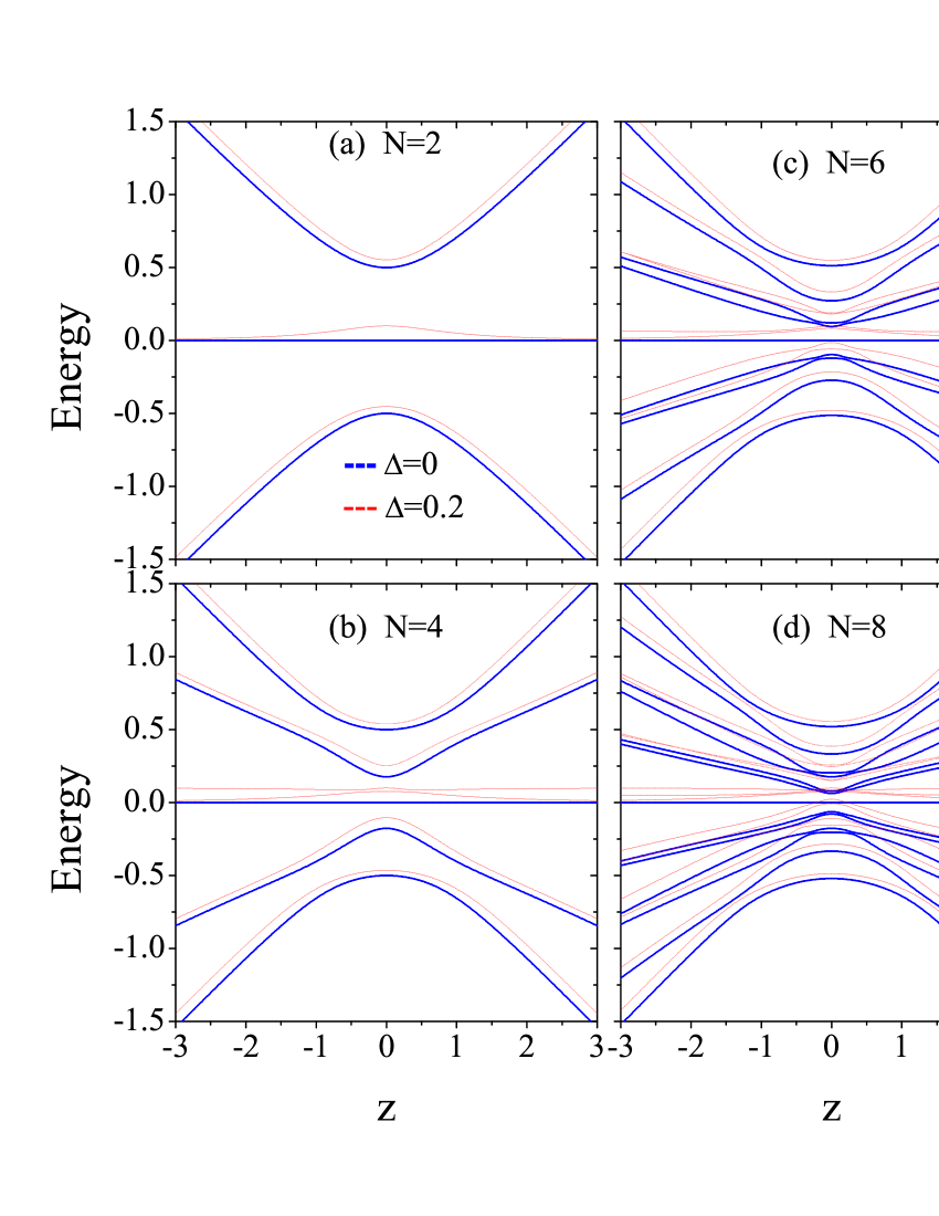
Figure 2: (Color online) Quantum energy levels for different particle numbers: (a) $N=2$, (b) $N=4$, (c) $N=6$, and (d) $N=8$. The thick and thin lines denote the cases $\Delta=0$ and $\Delta=0.2$, respectively. The energies are shown in units of $N\rho$ while the parameters $z$ and $\Delta$ are rescaled by $\rho$.

By directly diagonalizing the Hamiltonian matrix with a fixed $N$, we obtain the eigen-energy levels and the ground states of the system as shown in Figs. 2 and 3, respectively.

It is well known that a typical $\Lambda$-type three-level system supports dark-state solutions with zero eigenvalue puh07 ; linghy04 ; linghy07 . This type of state can result in a phenomenon known as coherent population trapping (CPT). For our system, when $\Delta=0$, from Figs. 2(b)-2(d) we see that the energy levels with energy value being zero are degenerate while other nonzero-energy levels are nondegenerate and are symmetrically distributed in both sides of the center level. This symmetrical energy structure is determined by the symmetry of the Hamiltonian $\hat{H}_{I}$ with $\phi=0$, i.e., the change of variables $(z,\rho)\rightarrow-(z,\rho)$ is equivalent to the unitary transformation $\hat{b}_{e}\rightarrow-\hat{b}_{e}$. In this case, the degeneracy of the zero-energy level (i.e., $d$) is given by

$$d=\lceil(\frac{N}{2}+1)/2\rceil=\frac{1}{4}(N-\mathrm{Mod}[N,4])+1,$$ (11)

the symbol $\lceil~{}\rceil$ stands for the ceiling function which maps a real number to the smallest following integer.

Notice that, if the parameter $\Delta$ has a perturbation, the above mentioned symmetry of the system with $\Delta=0$ will be broken. This leads to the energy levels shift and the zero-energy level splitting. For example, when $\Delta=0.2$ and $N=8$ [see Fig. 1(d)], all energy levels have been pushed up and the zero-energy level has split into three nonzero-energy levels. For different $N$, the maximum number of energy levels should be $(\tfrac{N}{2}+1)(\tfrac{N}{2}+2)/2$.

Figure 3: (Color online) Atomic fraction in the ground state versus the parameter $z$ with $\Delta=0$ and $\Delta=0.5$. Both $z$ and $\Delta$ are rescaled by $\rho$.

Now we discuss the ground-state properties which are closely associated with the QPT in the system. On one hand, by diagonalizing the Hamiltonian $\hat{H}_{I}$ numerically, both for $\Delta=0$ and for $\Delta\neq 0$, we have calculated the ground states with different total atom numbers. The results for atomic population fraction (i.e., $N_{a}/N$) in the ground state are demonstrated in Fig. 3. We find that the atomic fraction in the ground state decreases and gradually approaches to zero as the ratio of the coupling strength between two molecular modes to that between atom mode and the molecular mode increases. On the other hand, we study the ground state from the mean-field perspective. Based on the model (5), we solve the mean-field ground state from the eigen-equation $H_{mf}(\bar{a}^{\ast},\bar{a})|\bar{\psi}\rangle=\Theta(\mu)|\bar{\psi}\rangle$ with $\mu$ being the chemical potential for atoms and $|\bar{\psi}\rangle$ being the eigenstate. For $\Delta=0$, $z\geq 0$, and $\rho>0$, we obtain the eigenvalue and the corresponding eigenfunction for the ground state as follows:

$$\mu_{0}= \left\{\begin{array}[]{cc}-{z\over 2},&z>2\rho,\\ -{(z^{2}-2\rho^{2})\sqrt{z^{2}+8\rho^{2}}\over 4\sqrt{3}\rho^{2}},&z<2\rho;\\ \end{array}\right.$$ (14)

$$|\bar{\psi_{0}}\rangle= \left\{\begin{array}[]{cc}\left(\begin{array}[]{c}0\\ {1\over 2}\\ -{1\over 2}\\ \end{array}\right),&z>2\rho,\\ \left(\begin{array}[]{c}{\sqrt{4-z^{2}/\rho^{2}}\over\sqrt{6}}\\ {z\over 4\rho}e^{-i\phi}\\ -{\sqrt{z^{2}+8\rho^{2}}\over 4\sqrt{3}\rho}e^{-i\phi}\\ \end{array}\right),&z<2\rho.\\ \end{array}\right.$$ (23)

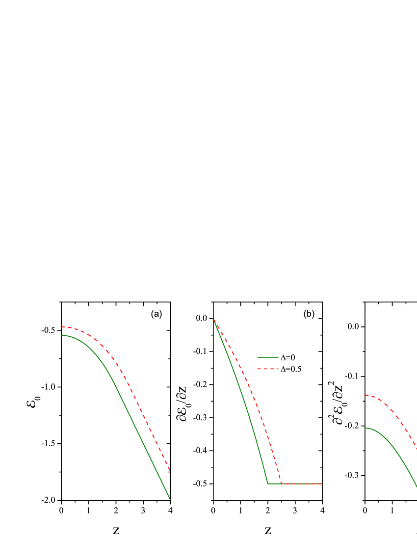
Figure 4: (Color online) The energy of the mean-field ground state (a) and its first (b) and second (c) derivatives with respect to coupling $z$. The parameters $z$ and $\Delta$ are rescaled by $\rho$.

For $\Delta\neq 0$, although the solutions to ground state can also be obtained analytically, the expressions are generally too messy to be instructive. We therefore simply display the results in Fig. 3. From Fig. 3 we find that, both for $\Delta=0$ and for $\Delta\neq 0$, the results for the quantum model (4) will tend to the analytical mean-field results with increasing the total particle number $N$.

It must be mentioned that, for our nonlinear system (5), the classical energy $\mathcal{E}$ does not equal the chemical potential, and the relation between them is $\mathcal{E}=\mu\pm\rho|\bar{b_{e}}||\bar{a}|^{2}$. We have calculated the ground-state energy $\mathcal{E}_{0}$ analytically and find its second derivative possesses a discontinuity at a critical point $z_{c}=2\rho+\Delta$ as demonstrated in Fig. 4. This divergence behavior implies that the system exists a second-order phase transition in the thermodynamic limit. When $z<z_{c}$ the system is in an atom-molecule mixture phase (i.e., $|\bar{a}|^{2}>0$) and when $z>z_{c}$ the system is in a pure molecule phase where $|\bar{a}|^{2}=0$. In the mixture phase, the asymptotic behavior of the ground state in the vicinity of the critical point with $\Delta=0$ is given by the variation of the parameter $s_{0}=|\bar{a}|^{2}$, i.e.,

$$s_{0}|_{z\rightarrow z_{c}}=\frac{1}{6}[4-z_{c}(2z-z_{c})].$$ (24)

IV Quantum phase transition

The previous calculations and analysis have demonstrated that the process of converting ultracold atoms to homonuclear diatomic molecules in bosonic system is a QPT which differs from the well-known BCS-BEC crossover phenomena in fermionic systems regalca2004 ; linksj2003 . Subsequently, we will describe and characterize this phase transition from different perspectives.

IV.1 Scaling laws

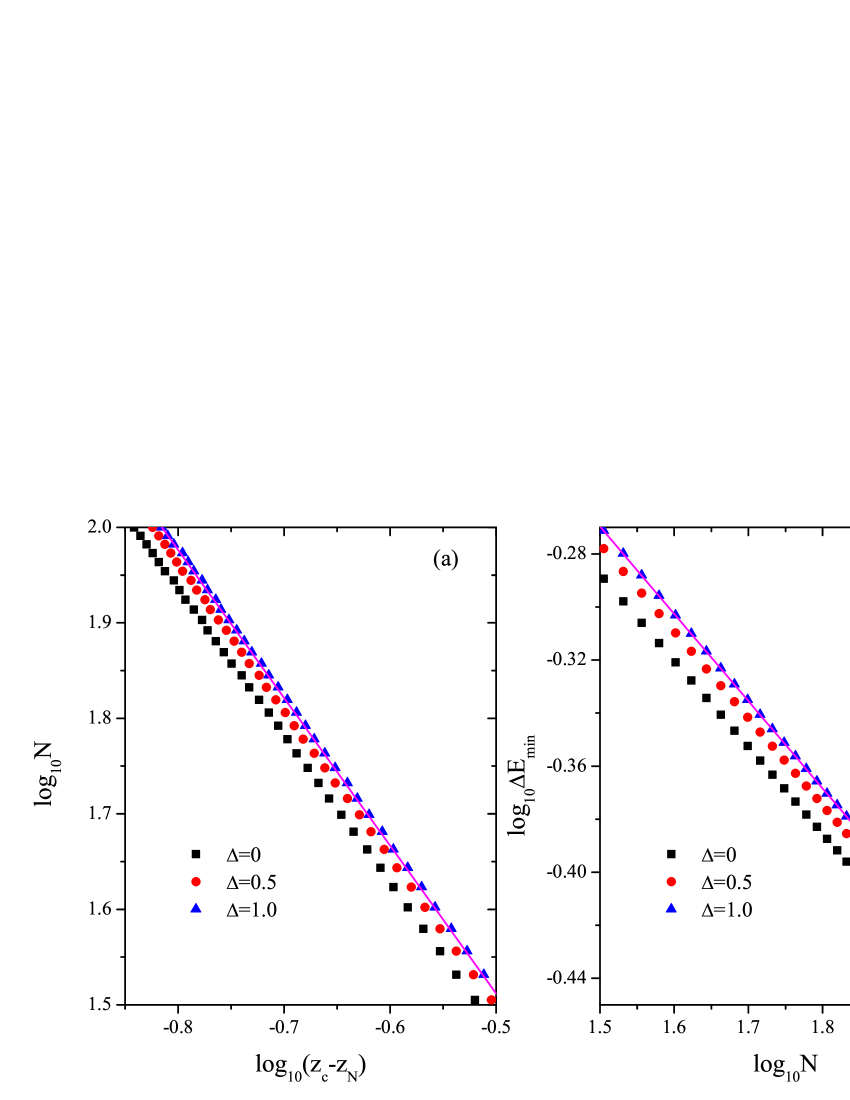
Figure 5: (Color online) (a) The total atomic number $N$ versus the offset between $z_{N}$ and $z_{c}$. (b) The minimum value of the energy gap (i.e., $\Delta E_{\mathrm{min}}$) at the pseudo-critical point $z_{N}$ versus $N$. Solid lines are plotted for guiding eyes, respectively, (from left to right) with the slopes being $-1.54764$ and $-0.32912$.

In order to understand the QPT in the system, we begin our discussion by analyzing the dimensionless energy gap between the first excited state and the ground state, namely, $\Delta E=(E_{1}-E_{0})/\rho$. With the help of diagonalizing the Hamiltonian (4) numerically, we have calculated the energy levels with different particle numbers. For a fixed $N$, the energy gap takes a minimum value at a point $z_{N}$ (it can be viewed as a pseudo-critical point of the $N$-particle system) and this point just corresponds to the position of avoided level crossing (see Fig. 2). Generally, the QPTs often occur at the positions of level crossings or avoided level crossings. For our avoided level crossings system, the existence of the minimum of energy gap indicates a basic signature of the phase transition. Similar to the phenomena studied in a two-level atom-molecule system santosg10 and in other systems, we find that, the gap $\Delta E$ in our system also tends to zero at a single point rather than over an interval of the dimensionless parameter $z/\rho$ with the particle number $N\rightarrow\infty$. This specific phenomenon implies that, when $N\rightarrow\infty$, the ground state is degenerate at the point $z_{c}$ where is no phase, which is a requirement for the occurrence of a broken-symmetry phase santosg10 .

To capture more features of the QPT in the system, we study the scaling behavior of the energy gap near the critical point. To this end, we first calculate the energy gap for different parameter $\Delta$ and the results have been plotted in Fig. 5. Either for the variation of the total atomic number $N$ versus $|z_{N}-z_{c}|$ [see Fig. 5(a)] or for the change of the minimum of the energy gap (i.e., $\Delta E_{\mathrm{min}}$) with respect to $N$ [see Fig. 5(b)], the same characteristic scaling laws have been observed for different $\Delta$, and different lines in each figures with a same slope gives the evidence.

In the quantum model (4), the total atom number $N$ can be regard as a correlation length scale of the system, and then one can connects this length scale to the offset between the pseudo-critical point and the critical point. Quantificationally, we have

$$\kappa|z_{c}-z_{N}|^{\nu}\simeq N^{-1},$$ (25)

where $\nu\simeq 1.54764$ is a critical exponent and $\kappa\simeq 0.18273$ is a inessential constant. This scaling law shows that the pseudo-critical point changes and tends as $N^{-1/\nu}$ toward the critical point and clearly approaches $z_{c}$ as $N\rightarrow\infty$ [see Fig. 5(a)]. From Fig. 5(b), we find another scaling law, that is

$$\Delta E_{\mathrm{min}}/N\simeq\Gamma N^{-\zeta},$$ (26)

where $\Gamma\simeq 1.67506$ is a constant. $\zeta\simeq 1.32912$ gives another important exponent, namely, the dynamic critical exponent. It must be mentioned that all constants and exponents given in the above two formulas are obtained in the case of $\Delta=0$, for other cases their values may have a slightly change. Comparing the product of two exponents in our system with that in a two-level atom-molecule system lisc11a we find that the values are obviously different. This difference indicates that the above two models belong to different universality classes.

IV.2 Fidelity

Similar to other concepts, the behavior of the fidelity can also be employed to identify the phase transition zanardip2006 ; zhouhq2008 . The fidelity is a measure of the distance between two states and this concept has been widely used in the field of quantum information nielsenma200 .

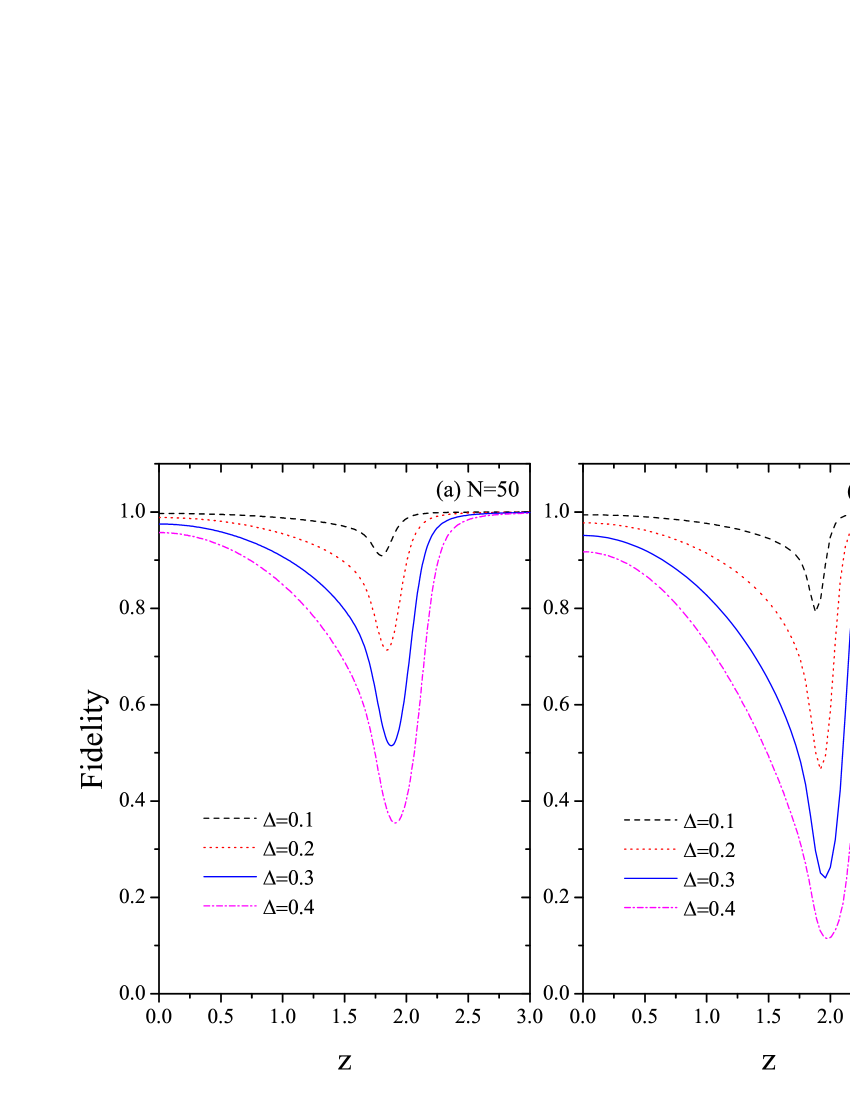
Figure 6: (Color online) Ground-state fidelity versus the parameter $z$ with $N=50$ (a) and with $N=100$ (b) for different $\Delta$. The parameters $\Delta$ and $\rho$ are rescaled by $\rho$.

One can define the fidelity through the modulus of the wave functions overlap between two states, i.e.,

$$F(\psi_{1},\psi_{2})=|\langle\psi_{1}|\psi_{2}\rangle|.$$ (27)

Here we only focus on the behaviors of the fidelity between two ground states. One ground state is obtained when $\Delta=0$, namely, $|\Delta=0\rangle$, the other ground state is calculated by treating $\Delta$ as a perturbation parameter, denoted as $|\Delta\neq 0\rangle$. we have estimated the wave-function overlap between two ground states with different particle number $N$ and varying parameter $\Delta$. Figure 6 shows the fidelities between the ground state $|\Delta=0\rangle$ and the ground state $|\Delta=\alpha\rangle$ with $\alpha=0.1,0.2,0.3$, and $0.4$. Both for $N=50$ and for $N=100$ we see that the fidelity $|\langle\Delta=0|\Delta\neq 0\rangle|$ shows dip behavior at the point corresponding to the pseudo-critical point. The results imply that the two ground states are distinguishable and there is an obvious signal for the QPT as long as $\alpha\neq 0$. Moreover, we observe that the dip of the ground-state fidelity becomes deeper and the point where the fidelity has a minimum varies with increasing the value of $\alpha$, this phenomenon is very different from that in a two-level atom-molecule model where the fidelity has a minimum at the same point santosg10 . The reason is that, in our model the phase transition point $z_{c}$ is a function of the parameters $\rho$ and $\Delta$. For a larger value of $\alpha$, we find that the distinguishability of the two states increases and the minimum of the fidelity changes evidently.

Now we compare the results obtained in the case of $N=50$ with the results for $N=100$. For a same $\Delta$, it is seen that the position of the minimum fidelity for $N=100$ is closer to the critical point $z_{c}$ than that for $N=50$. In fact we have calculated the ground-state fidelity with varying the particle number $N$ and find that, for a fixed $\alpha$, with increasing $N$, the wave functions overlap between the two states become smaller (i.e., the two states are more distinguishable) and the position where the minimum fidelity occurs moves toward $2\rho+\Delta$. Thus in the finite particle number case the occurrence of the minima of the fidelity gives a information about the phase transition in the system.

IV.3 Geometric phase

In this subsection we convert to investigate the behavior of the ground-state geometric phase starting from the mean-field model (5). In the following study we only focus our attention on the situation that the detuning is absent (i.e., $\Delta=0$). Because the analytical results can be obtained in this case. To employ the procedures for calculating geometric phase in nonlinear systems proposed in Refs. liuj2010 ; fulb2010 , we introduce some new variables through setting $a=\sqrt{1-2(p_{1}+p_{2})}e^{i\lambda},b_{g}=\sqrt{p_{1}}e^{i(2\lambda+q_{1})}$, and $b_{e}=\sqrt{p_{2}}e^{i(2\lambda+q_{2})}$, where $\lambda=\arg(a)$ denotes the total phase, $p_{1}=|b_{g}|^{2}$ and $p_{2}=|b_{e}|^{2}$ are the population probabilities of the ground state and excited state molecules, respectively, $q_{1}=\arg(b_{g})-2\arg(a)$ and $q_{2}=\arg(b_{e})-2\arg(a)$ measure the relative phases. With the help of these new variables, the three-level system can be cast into a classical Hamiltonian

$$\mathcal{H}= 2z\sqrt{p_{1}p_{2}}\cos(q_{1}-q_{2})$$

$$+2\rho\sqrt{p_{2}}[1-2(p_{1}+p_{2})]\cos(q_{2}+\phi).$$ (28)

The Schrödinger equations (5) together with the normalization condition lead to

$$\frac{d\lambda}{dt}=-2\rho\sqrt{p_{2}}\cos(q_{2}+\phi),$$ (29)

and

$$\frac{dp_{i}}{dt}=-\frac{\partial\mathcal{H}}{\partial q_{i}},~{}~{}~{}\frac{dq_{i}}{dt}=\frac{\partial\mathcal{H}}{\partial p_{i}},$$ (30)

with $i=1,2$. These four equations have established a connection between the projected Hilbert space spanned by $\mathbf{S}(p_{i},q_{i})$ and the parameter space spanned by $\mathbf{R}(z,\rho,\phi)$.

Now we calculate the geometric phase for the ground state of the system. For simplicity, we construct a closed loop $C$ in the parameter space by treating $z$ and $\rho$ as constants and varying $\phi$ with time from $0$ to $2\pi$. The system is assumed to evolve adiabatically along the cyclic path with a rate $\epsilon\sim|{d\phi\over dt}|\sim{\frac{1}{T}}$, where $T$ is the period of the cyclic evolution. Initially, we prepare the system in the ground state of $H_{mf}(\phi=0)$, after a cyclic adiabatic evolution, the state will acquire a geometric phase besides the dynamical phase. Here it is noted that the adiabatic parameter $\epsilon\ll{1}$, and thus it can be regarded as a small parameter during the process for determining the geometric phase. Following the method in Ref. liuj2010 , we expand the total phase $\lambda$ in a perturbation series in $\epsilon$, i.e.,

$${d\lambda\over dt}=\lambda_{0}(\epsilon^{0})+\lambda_{1}(\epsilon^{1})+O(\epsilon^{2}),$$ (31)

to separate the pure geometric part from the total phase. The time integrals of the zero-order term and the first-order term in Eq. (31) will respectively give the dynamic phase and the geometric phase in the adiabatic limit $\epsilon\rightarrow 0$ or $T\rightarrow\infty$, and the contribution from the higher-order terms will vanish.

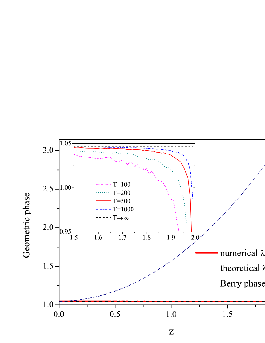
Figure 7: (Color online) Comparison between the numerical results for the ground-state geometric phase with $T=500$ and the analytical results given by Eq. (36). The dotted line denotes the results obtained from Berry’s formula. The inset illustrates the numerical results around the critical point with different $T$. The parameter $z$ is rescaled by $\rho$.

During the adiabatic evolution the system will fluctuate around the ground state due to the small but finite value of $\epsilon$. This fact allows us to make expansions as $p_{i}=\bar{p}_{i}(\mathbf{R})+\delta{p}_{i}(\mathbf{R})$ and $q_{i}=\bar{q}_{i}(\mathbf{R})+\delta{q}_{i}(\mathbf{R})$ with $i=1,2$, where $(\bar{p}_{i},\bar{q}_{i})$ stand for the instantaneous ground state, $\delta p_{i}$ and $\delta q_{i}$ denote the fluctuations induced by the slow change of the system. Substituting these expressions back into Eq. (29), when $z<2\rho$, we have

$$\lambda_{0}= -\mu_{0}(\mathbf{R}),$$ (32)

$$\lambda_{1}= {-2\bar{p}_{2}\sqrt{\bar{p}_{1}}z+\rho[\bar{p}_{2}(6\bar{p}_{2}+6\bar{p}_{1}-1)+\delta{p}_{2}]\over\sqrt{\bar{p}_{2}}},$$ (33)

where the chemical potential of the ground state can be expressed as $\mu_{0}=-2z\sqrt{\bar{p}_{1}\bar{p}_{2}}-3\rho\sqrt{\bar{p}_{2}}[1-2(\bar{p}_{1}+\bar{p}_{2})]$. Moreover, from Eqs. (30), we have

$$\delta{p}_{2}=\frac{2\sqrt{\bar{p}_{2}}(z\bar{p}_{2}+z\bar{p}_{1}-4\rho\bar{p}_{1}^{3/2})}{\rho[z(1+6\bar{p}_{2}+6\bar{p}_{1})-16\rho\bar{p}_{1}^{3/2}]}\frac{d\phi}{dt}.$$ (34)

To deduce Eqs. (33) and (34), we have used the fixed-point equations ${\partial\mathcal{H}\over\partial{p}_{i}}|_{(\bar{p}_{i},\bar{q}_{i})}=0$ and the condition ${d\over dt}\delta{q}_{i}\sim O(\epsilon^{2})$. Combining Eq. (34) with Eq. (33), and then using the fixed-point values corresponding to the ground state, i.e., $(\bar{p}_{1},\bar{q}_{1};\bar{p}_{2},\bar{q}_{2})=(\tfrac{z^{2}}{16\rho^{2}},\bar{q}_{2}\pm\pi;\tfrac{z^{2}+8\rho^{2}}{48\rho^{2}},\pm\pi-\phi)$, we obtain

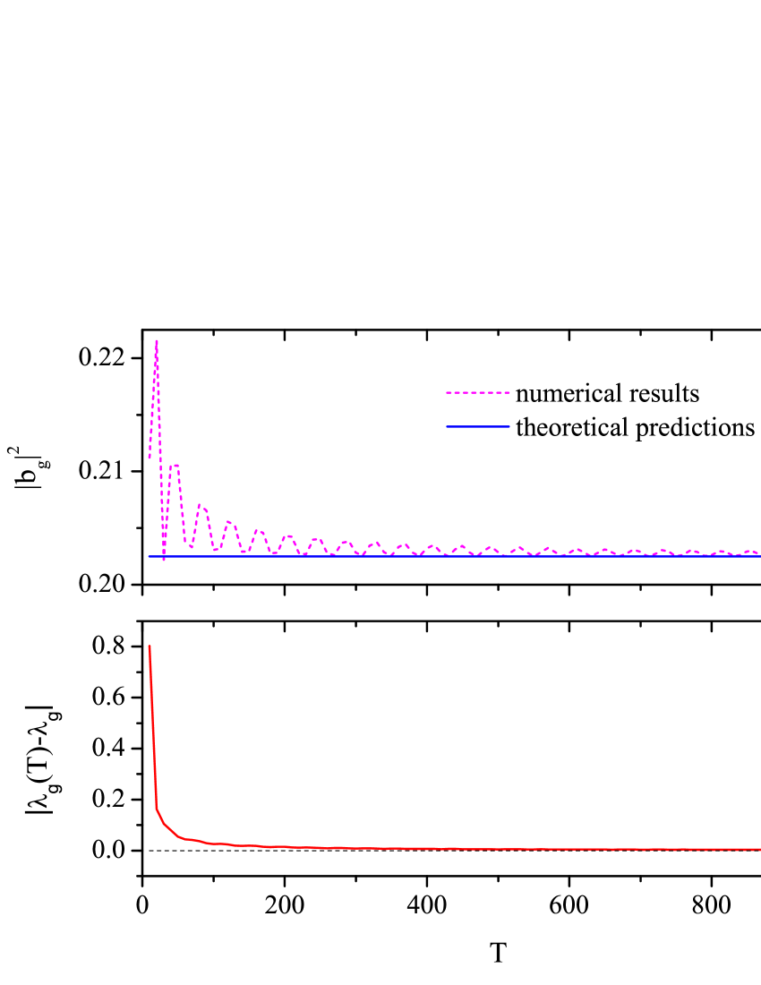
Figure 8: (Color online) The convergence of population in the ground-state molecular mode (a) and the geometric phase (b) with respect to the evolution period $T$ for $z/\rho=1$.

$$\lambda_{1}={1\over 6}{d\phi\over dt}.$$ (35)

By integrating Eq. (35) over $T$ with respect to time, we have

$$\lambda_{g}=\int_{0}^{T}\lambda_{1}dt={1\over 6}\int_{0}^{2\pi}{d\phi}=\frac{\pi}{3}.$$ (36)

As a comparison we give the result that is directly calculated from the Berry’s formula berrymv1984 , i.e.,

$$\lambda_{b}=i\int_{0}^{2\pi}\langle\bar{\psi_{0}}|\nabla_{\phi}|\bar{\psi_{0}}\rangle{d\phi}=\frac{\pi}{6}\left(2+\frac{z^{2}}{\rho^{2}}\right).$$ (37)

Now we consider the situation when $z>2\rho$. In this case, the ground state, i.e., $\bar{p}_{1}=\bar{p}_{2}=1/4$, is independent of the parameter $\mathbf{R}$. Simple calculations from Eqs. (29) and (30) lead to

$${d\lambda\over{dt}}={z\over 2}=-\mu_{0},$$ (38)

and then

$$\lambda=\int_{0}^{T}\lambda_{0}dt=-\int_{0}^{T}\mu_{0}{dt}=\lambda_{d}.$$ (39)

This result implies that the geometric phase $\lambda_{g}=0$ in the case $z>2\rho$. To sum up, our above theoretical calculations demonstrate that the mean-field geometric phase of the ground state jumps from zero to $\pi/3$ when the system undergoes the phase transition from a mixture phase to a pure molecular phase. These analytical predictions have been checked by numerically solving Eq. (5) or Eqs. (29) and (30) as illustrated in Fig. 7. We see that, if the evolution period $T$ is large enough, the simulated results show a good agreement with the analytical predictions. We use Fig. 8 to exhibit the convergence behaviors of the ground-state and the geometric phase with increasing $T$, and a large convergence rate has been observed. It is worth emphasizing that, the different values of the geometric phase in different parameter regions can be an evident signature of the QPT in the system.

V Conclusion

We have investigated the quantum phase transition in a three-level atom-molecule conversion system. By using different approaches we show that the system exists a second-order phase transition similar to a QPT exhibited in a two-level bosonic model santosg10 . Firstly, though analyzing the properties of energy gap we derive two scaling laws and the corresponding critical exponents. It is found that the two-level model and our model belong to different universality classes. Secondly, we discuss the ground-state fidelity. A minimum value of the fidelity near the critical point has been found. Finally, we have calculated the ground-state geometric phase and a discontinues behavior at the critical point has been observed. This phenomenon is similar to that studied in a system of a Bose-Einstein condensate in an optical cavity lisc11b . It establishes a connection between the ground-state geometric phase and the QPT in an interacting atom-molecule bosonic model following the early works in spin-chain systems Carolloacm2005 ; zhusl2006 . In summary, we have demonstrated novel characteristic scaling laws and abrupt change of the ground-state geometric phase in the vicinity of the critical point, which give the pronounced signals toward the existence of a QPT in the system.

References

- (1) S. Sachdev, Quantum Phase Transitions (Cambridge University Press, Cambridge, 1999); M. Vojta, Rep. Prog. Phys. 66, 2069 (2003).
- (2) S. L. Sondhi, S. M. Girvin, J. P. Carini, and D. Shahar, Rev. Mod. Phys. 69, 315 (1997).
- (3) M. Greiner, O. Mandel, T. Esslinger, T. W. Hänsch, and I. Bloch, Nature 415, 39 (2002).
- (4) D. Tilahun, R. A. Duine, and A. H. MacDonald, Phys. Rev. A 84, 033622 (2011).
- (5) See, e.g., L. Pitaevskii and S. Stringari, Bose-Einstein Condensation (Clarendon Press, Oxford, 2003).
- (6) J. Ruseckas, G. Juzeliūnas, P. Öhberg, and M. Fleischhauer, Phys. Rev. Lett. 95, 010404 (2005).
- (7) E. A. Donley, N. R. Claussen, S. T. Thompson, and C. E. Wieman, Nature (London) 417, 529 (2002).
- (8) K. Xu, T.Mukaiyama, J. R. Abo-Shaeer, J. K. Chin, D. E. Miller, and W. Ketterle, Phys. Rev. Lett. 91, 210402 (2003).
- (9) J. Herbig, T. Kraemer, M. Mark, T. Weber, C. Chin, H.-C. Nägerl, and R. Grimm, Science 301, 1510 (2003).
- (10) R. Wynar, R. S. Freeland, D. J. Han, C. Ryu, and D. J. Heinzen, Science 287, 1016 (2000).
- (11) T. Rom, T. Best, O. Mandel, A. Widera, M. Greiner, T. W. Hänsch, and I. Bloch, Phys. Rev. Lett. 93, 073002 (2004).
- (12) K. Winkler, G. Thalhammer, M. Theis, H. Ritsch, R. Grimm, and J. H. Denschlag, Phys. Rev. Lett. 95, 063202 (2005).
- (13) U. Gaubatz, P. Rudecki, M. Becker, S. Schiemann, M. Külz, and K. Bergmann, Chem. Phys. Lett. 149, 463 (1988).
- (14) J. R. Kuklinski, U. Gaubatz, F. T. Hioe, and K. Bergmann, Phys. Rev. A 40, 6741 (1989).
- (15) E. Pazy, I. Tikhonenkov, Y. B. Band, M. Fleischhauer, and A. Vardi, Phys. Rev. Lett. 95, 170403 (2005).
- (16) H. Y. Ling, P. Maenner, W. Zhang, and H. Pu, Phys. Rev. A 75, 033615 (2007).
- (17) E. A. Shapiro, M. Shapiro, AviPe’er, and J. Ye, Phys. Rev. A 75, 013405 (2007).
- (18) S.-Y. Meng, L.-B. Fu, and J. Liu, Phys. Rev. A 78, 053410 (2008).
- (19) L. B. Fu and J. Liu, Ann. Phys. 325, 2425 (2010).
- (20) F. Cui and B. Wu, Phys. Rev. A 84, 024101 (2011).
- (21) G. Santos, A. Foerster, J. Links, E. Mattei, and S. R. Dahmen, Phys. Rev. A 81, 063621 (2010).
- (22) S. C. Li and L. B. Fu, Phys. Rev. A 84, 023605 (2011).
- (23) H. Pu, P. Maenner, W. Zhang, and H. Y. Ling, Phys. Rev. Lett. 98, 050406 (2007).
- (24) H. Y. Ling, H. Pu, and B. Seaman, Phys. Rev. Lett. 93, 250403 (2004).
- (25) H. Y. Ling, P. Maenner, W. Zhang, and H. Pu, Phys. Rev. A 75, 033615 (2007).
- (26) C. A. Regal, M. Greiner, and D. S. Jin, Phys. Rev. Lett. 92, 040403 (2004); G. B. Partridge, K. E. Strecker, R. I. Kamar, M. W. Jack, and R. G. Hulet, ibid. 95, 020404 (2005).
- (27) J. Links, H. Q. Zhou, R. H. McKenzie, and M. D. Gould, J. Phys. A 36, R63 (2003); G. Santos, A. Tonel, A. Foerster, and J. Links, Phys. Rev. A 73, 023609 (2006); J. Li, D. F. Ye, C. Ma, L. B. Fu, and J. Liu, ibid. 79, 025602 (2009).
- (28) P. Zanardi and N. Paunković, Phys. Rev. E 74, 031123 (2006).
- (29) H.-Q. Zhou and J. P. Barjaktarevic, J. Phys. A 41, 412001 (2008).
- (30) M. A. Nielsen and I. L. Chuang, Quantum Computation and Quantum Information (Cambridge University Press, Cambridge, UK, 2000).
- (31) J. Liu and L. B. Fu, Phys. Rev. A 81, 052112 (2010).
- (32) M. V. Berry, Proc. R. Soc. London, Ser. A 392, 45 (1984).
- (33) S. C. Li, L. B. Fu, and J. Liu, Phys. Rev. A 84, 053610 (2011).
- (34) A. C. M. Carollo and J. K. Pachos, Phys. Rev. Lett. 95, 157203 (2005).
- (35) S.-L. Zhu, Phys. Rev. Lett. 96, 077206 (2006).