Corrections to our results for optical nanofiber traps in Cesium

Abstract

Several errors in Refs. lacroute2012 ; goban2012 are corrected related to the optical trapping potentials for a state-insensitive, compensated nanofiber trap for the $D_{2}$ transition of atomic Cesium. Section I corrects our basic formalism in Ref. lacroute2012 for calculating dipole-force potentials. Section II corrects erroneous values for a partial lifetime and a transition wavelength in Ref. lacroute2012 . Sections III and IV present corrected figures for various trapping configurations considered in Refs. lacroute2012 and goban2012 , respectively.

I Formalism

The light shifts calculated in Ref. lacroute2012 are based upon Eq. (2) in Ref. lacroute2012 . The text states that the basis for Eq. (2) is ‘spherical’ (i.e., irreducible spherical tensors). In fact, the basis for Eq. (2) is actually a Cartesian basis (i.e., $x,y,z$), which we used to perform all calculations in Ref. lacroute2012 .

In Eq. (2) of Ref. lacroute2012 , $\alpha^{(0)}$,$\alpha^{(1)}$ and $\alpha^{(2)}$ are the scalar, vector and tensor atomic dynamic polarizabilities defined in Ref. deutsch . The dipole matrix element in Ref. lacroute2012 is $d_{JJ^{\prime}}^{2}=|\left\langle J||\mathbf{d}||J^{\prime}\right\rangle|^{2}=\frac{3\pi\epsilon_{0}\hbar c^{3}}{\omega_{J^{\prime}J}^{3}}\frac{2J^{\prime}+1}{2J+1}\frac{1}{\tau_{J^{\prime}J}}$, as defined in Ref. dstecktext . However, as Ref. deutsch only considered light shifts of the ground states, the definition for $d_{JJ^{\prime}}$ in Ref. dstecktext becomes problematic when defining $d_{JJ^{\prime}}$ for the excited states. $J$ and $J^{\prime}$ are defined with respect to states of lower to higher energy, respectively, rather than with respect to initial and final states. This notation is therefore ambiguous if the initial state is an excited state. Also, the counter-rotating term was not taken into account in Ref. deutsch . Therefore, we follow the formalism in Refs. rosenbusch ; Beloy2009 ; fam2012 , in which case Eq. (2) of Ref. lacroute2012 should be rewritten as follows:

$$\begin{array}[]{llll}\hat{H}_{\mathrm{ls}}&=-\alpha^{(0)}\mathbf{\hat{E}^{(-)}}\cdot\mathbf{\hat{E}^{(+)}}-i\alpha^{(1)}\frac{\left(\mathbf{\hat{E}^{(-)}}\times\mathbf{\hat{E}^{(+)}}\right)\cdot\mathbf{\hat{F}}}{2F}-\sum\limits_{\mu,\nu}\alpha^{(2)}\hat{E}^{(-)}_{\mu}\hat{E}^{(+)}_{\nu}\frac{3}{F(2F-1)}\left[\frac{1}{2}(\hat{F}_{\mu}\hat{F}_{\nu}+\hat{F}_{\nu}\hat{F}_{\mu})-\frac{1}{3}\hat{F}^{2}\delta_{\mu\nu}\right],\end{array}$$ (1)

where the dipole matrix element in Refs. rosenbusch ; Beloy2009 ; fam2012 is $d_{JJ^{\prime}}^{2}=|\left\langle J||\mathbf{d}||J^{\prime}\right\rangle|^{2}=\frac{3\pi\epsilon_{0}\hbar c^{3}}{\omega_{J^{\prime}J}^{3}}(2J^{\prime}+1)\frac{1}{\tau_{J^{\prime}J}}$, where $(J,J^{\prime})$ are for (lower, upper) levels, respectively. $\alpha^{(0)}$, $\alpha^{(1)}$, and $\alpha^{(2)}$ of Eq. (1) include counter-rotating terms. However, in Ref. lacroute2012 , we made an error in the definition of the vector polarizability, $\alpha^{(1)}$, by neglecting the rank dependence of the counter-rotating terms. In this errata, we correct the definition of $\alpha^{(1)}$ to incorporate the rank dependence of the counter-rotating terms in our calculations of light shifts rosenbusch ; Beloy2009 ; fam2012 .

The dynamic polarizabilities are then given by

$$\alpha^{(0)}(J,F) = \displaystyle\sum\limits_{nJ^{\prime}F^{\prime}}\frac{d_{JJ^{\prime}}^{2}}{3}(2F^{\prime}+1)\begin{Bmatrix}J&J^{\prime}&1\\ F^{\prime}&F&I\end{Bmatrix}^{2}G^{(0)}_{FF^{\prime}}$$ (2)

$$\alpha^{(1)}(J,F) = 2\displaystyle\sum\limits_{nJ^{\prime}F^{\prime}}(-1)^{F+F^{\prime}}d_{JJ^{\prime}}^{2}\sqrt{\frac{3F(2F+1)}{2(F+1)}}\begin{Bmatrix}1&1&1\\ F&F&F^{\prime}\end{Bmatrix}$$ (3)

$$\times(2F^{\prime}+1)\begin{Bmatrix}J&J^{\prime}&1\\ F^{\prime}&F&I\end{Bmatrix}^{2}G^{(1)}_{FF^{\prime}}$$

$$\alpha^{(2)}(J,F) = \displaystyle\sum\limits_{nJ^{\prime}F^{\prime}}(-1)^{F+F^{\prime}}d_{JJ^{\prime}}^{2}\sqrt{\frac{10F(2F+1)(2F-1)}{3(F+1)(2F+3)}}\begin{Bmatrix}1&1&2\\ F&F&F^{\prime}\end{Bmatrix}$$ (4)

$$\times(2F^{\prime}+1)\begin{Bmatrix}J&J^{\prime}&1\\ F^{\prime}&F&I\end{Bmatrix}^{2}G^{(2)}_{FF^{\prime}},$$

where $G^{(K)}_{ij}$ is the rank-$K$ propagator defined as

$$G^{(K)}_{ij}=\frac{1}{\hbar}\left\{\frac{1}{\omega_{ji}-\omega}+\frac{(-1)^{K}}{\omega_{ji}+\omega}\right\}.$$ (5)

We note that the counter-rotating term gains an overall minus sign for $K=1$ in the expression for the vector propagator $G_{FF^{\prime}}^{(1)}$. We have confirmed that our corrected formula for the dynamic polarizabilities (i.e., Eqs. (1-5)) is now consistent with the expressions in Ref. rosenbusch .

II Partial Lifetimes and Transition Wavelengths

In addition to corrections to our formalism discussed above, we correct two numerical errors for the atomic data used to calculate the light shifts in Refs. lacroute2012 ; goban2012 . These errors stem from a mistake for a partial lifetime $\tau$ and from an error for a transition wavelength $\lambda$. All values for $\tau$ and $\lambda$ of Ref. lacroute2012 were taken from Tables 7.1–7.3 of J. McKeever’s Ph.D Thesis mckeever . The specific errors are as follows:

1. The wavelength for the transition $7S_{1/2}\leftrightarrow 6P_{3/2}$ in Table 7.2 of Ref. mckeever is listed as $469.5$ nm, whereas the correct value is $1469.5$ nm.

2. The partial lifetime for the transition $7D_{3/2}\leftrightarrow 6P_{3/2}$ in Table 7.3 of Ref. mckeever is listed as $709.7$ $\mu$s, but instead should be $0.7097$ $\mu$s.

The corrected values for Tables 7.1–7.3 of Ref. mckeever are highlighted with green color in Tables 1 and 2 of this errata.

The partial lifetimes and wavelengths from Table 7.1–7.3 of Ref. mckeever were obtained from Refs. laplanche ; fabry with the exception of the values for $6P\rightarrow 6S$ from Ref. dsteck and $6D\rightarrow 6P$ from Ref. christina .

To further confirm the accuracy of the corrected values from Ref. mckeever , we refer to Tables V and VI of Arora et al. arora2007 (heretofore, labelled as ‘Clark’). Tables 1 and 2 in this errata compare the corrected tables from Ref. mckeever to Tables V–VI of Ref. arora2007 . Our values agree well with those from Ref. arora2007 .

We note that all previous publications prior to Ref. lacroute2012 from our group, including Ref. mckeeverprl , have used the correct values in Tables 1–2 and not those from McKeever’s thesis mckeever . Furthermore, these earlier results are for linearly polarized trapping fields for which the contribution of the vector term $\alpha^{(1)}$ vanishes. Therefore, these earlier results from our group stand without revision.

Using the revised formalism from Section I and based on the corrected numerical values in Tables 1–2 from Section II, we present corrected figures to replace those in Refs. lacroute2012 ; goban2012 as described in the following sections.

III Corrected Figures for Ref. lacroute2012

The figure numbering in this errata mirrors that of Ref.lacroute2012 with corrected figures given here in Roman numerals. Fig. VIlacroute2012 relates to magic wavelengths for the Cs $D_{2}$ line and replaces Fig. 6 in Ref. lacroute2012 . The magic wavelength in this note is defined by the weighted average of the Zeeman sublevels $m_{F}$ (i.e., not by $\alpha^{(0)}$ alone).

As in Ref. lacroute2012 , we include a surface interaction potential of an atom with the dielectric nanofiber in our calculation of the total atomic trap potential. The surface potential of the ground state Cs atom near a planar dielectric surface can be approximated by the van der Waals potential $-\frac{C_{3}}{d^{3}}$, where $d=r-a$ and $C_{3}/\hbar=1.16~{}\text{kHz }\mu\text{m}^{3}$ lacroute2012 ; stern2011 .

In Figs. IXlacroute2012 , IXlacroute2012 , and IXlacroute2012 , the two-color evanescent trap from Ref. vetsch2010 is constructed from a pair of counter-propagating $x$-polarized ($\varphi_{0}=0$) red-detuned beams ($P_{\text{red}}=2\times 2.2$ mW) at $\lambda_{\text{red}}=1064$ nm, forming an optical lattice, and a single repulsive $y$-polarized ($\varphi_{0}=\pi/2$) blue-detuned beam ($P_{\text{blue}}=25$ mW) at $\lambda_{\text{blue}}=780$ nm. The SiO₂ tapered optical fiber has radius $a=250$ nm in the trapping region. Figs. IXlacroute2012 ,IXlacroute2012 , IXlacroute2012 replace figures of Fig. 7, 8, 9 of Ref. lacroute2012 .

For the magic, compensated trap in Figs. Xlacroute2012 , XIlacroute2012 , XIIlacroute2012 , we use a pair of counter-propagating $x$-polarized ($\varphi_{0}=0$) red-detuned beams ($P_{\text{red}}=2\times 0.95$ mW) at the magic wavelength $\lambda_{\text{red}}=935.3$ nm. Counter-propagating, $x$-polarized blue-detuned beams at a second magic wavelength $\lambda_{\text{blue}}=684.9$ nm are used with a power $P_{\text{blue}}=2\times 16$ mW. The resulting interference is averaged out by detuning the beams to $\delta_{fb}=30$ GHz. Figs. Xlacroute2012 , XIlacroute2012 , XIIlacroute2012 replace Figs. 10, 11, 12 of Ref. lacroute2012 .

IV Corrected Figures for Ref. goban2012

Because of the errors described in Sections I and II, our experiment in Ref. goban2012 used red- and blue-detuned beams at wavelengths $\lambda_{\text{red}}=937.1$ nm and $\lambda_{\text{blue}}=686.1$ nm instead of the correct values of $\lambda_{\text{red}}\simeq 935.7$ nm and $\lambda_{\text{blue}}\simeq 684.8$ nm calculated in the same fashion as Fig. VIlacroute2012 but now for $F=4$ of $6S_{1/2}$ to $F^{\prime}=5$ of $6P_{3/2}$. Fig. Agoban2012 shows the trapping potentials for the ground and excited states for the correct magic wavelengths of $\lambda_{\text{red}}\simeq 935.7$ nm and $\lambda_{\text{blue}}\simeq 684.8$ nm for this transition.

For the actual wavelengths $\lambda_{\text{red}}=937.1$ nm and $\lambda_{\text{blue}}=686.1$ nm used in our experiment goban2012 , Fig.1 and Fig. SM5 of Ref. goban2012 are here replaced by Figs. Bgoban2012 and Cgoban2012 , respectively, which incorporate the revisions described in Sections I and II.

V Conclusion

Our emphasis has been to correct the formalism (Section I) and atomic data (Section II and Tables I, II) that are the basis for our calculations in Refs. lacroute2012 ; goban2012 . Recently a more extensive set of atomic data than in Tables I and II has become available fam2012 . We have confirmed that these data with our formalism in Eqs. (1-5) reproduce Figs. (4, 5) from Ref. fam2012 .

However, the expanded set of atomic levels and lifetimes in Ref. fam2012 lead to small differences between Figs. (4, 5) fam2012 and corresponding figures computed from our Tables I, II. These differences are most pronounced around $685$nm (e.g., our Fig. VI(a)) principally due to excited-state contributions up to $n\sim 25$, which are not included in Tables I, II. We therefore recommend that the data set from Ref. fam2012 be employed for the calculation of ac Stark shifts for the $D_{2}$ line in atomic Cesium rather than the less extensive data in our Tables I, II.

Level $nS$	$\lambda_{\text{McKeever}}$	$\lambda_{\text{Clark}}$	$\tau_{\text{McKeever}}$	$\tau_{\text{Clark}}$
	(nm)	(nm)	($\mu$s)	($\mu$s)
6	852.4	852.35	0.03051	0.0306
7	1469.5	1469.89	0.07529	0.0749
8	794.4	794.61	0.2599	0.2319
9	658.8	658.83	0.5533	0.4759
10	603.4	603.58	0.9924	0.8374
11	574.6		1.607
12	557.3		2.428
13	546.3		3.49
14	538.5		4.809
15	532.9		6.431

Table 1: Comparison between corrected partial lifetimes in Ref. mckeever with Ref. arora2007 for $6P_{3/2}\rightarrow 6S_{1/2}$ dsteck and $nS_{1/2}\rightarrow 6P_{3/2}$ for $n=7-15$ laplanche . Partial lifetime ($\tau_{\text{McKeever}}$) and wavelength ($\lambda_{\text{McKeever}}$) are from Ref. mckeever with the corrected value highlighted in green. $\tau_{\text{Clark}}$ and $\lambda_{\text{Clark}}$ are from Ref. arora2007 . The conversion from $d$ to $\tau$ from Ref. arora2007 is done using Eq. (7.8) in Ref. mckeever .

Level $nD$	$\lambda_{3/2~{}\text{McKeever}}$	$\lambda_{3/2~{}\text{Clark}}$	$\tau_{3/2~{}\text{McKeever}}$	$\tau_{3/2~{}\text{Clark}}$	$\lambda_{5/2~{}\text{McKeever}}$	$\lambda_{5/2~{}\text{Clark}}$	$\tau_{5/2~{}\text{McKeever}}$	$\tau_{5/2~{}\text{Clark}}$
	(nm)	(nm)	($\mu$s)	($\mu$s)	(nm)	(nm)	($\mu$s)	($\mu$s)
5	3612.7	3614.09	10.09	9.2931	3489.2	3490.97	1.433	1.3692
6	921.1	921.11	0.3466	0.3497	917.2	917.48	0.0587	0.0604
7	698.3	698.54	0.7097	0.7061	697.3	697.52	0.1198	0.1203
8	621.7	621.93	1.284	1.2884	621.3	621.48	0.217	0.1566
9	584.7		2.131		584.5		0.3587
10	563.7		3.29		563.5		0.5527
11	550.4		4.807		550.3		0.8063

Table 2: Comparison between corrected partial lifetimes in Ref. mckeever with Ref. arora2007 for $nD_{(3/2,5/2)}\rightarrow 6P_{3/2}$. Partial lifetime ($\tau_{(3/2,5/2)~{}\text{McKeever}}$) and wavelength ($\lambda_{(3/2,5/2)~{}\text{McKeever}}$) are from Ref. mckeever with the corrected value highlighted in green. $\tau_{(3/2,5/2)~{}\text{Clark}}$ and $\lambda_{(3/2,5/2)~{}\text{Clark}}$ are from Ref. arora2007 . The conversion from $d$ to $\tau_{(3/2,5/2)}$ from Ref. arora2007 is done using Eq. (7.8) in Ref. mckeever .

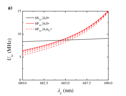
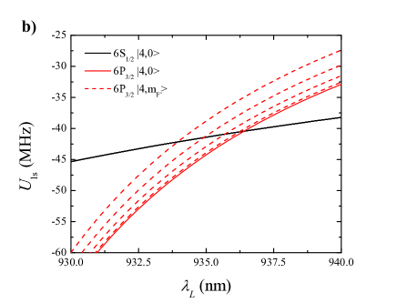
Figure VIlacroute2012 : Replacement for Fig. 6 in Ref. lacroute2012 for determination of the magic wavelengths for the $6S_{1/2},F=4\rightarrow 6P_{3/2},F^{\prime}=4$ transition of the Cs $D_{2}$ line. The light shifts $U_{ls}$ are for a linearly polarized beam with constant intensity $2.9\times 10^{9}~{}\text{W m}^{-2}$ around (a) the blue-detuned magic wavelength at $\lambda_{\text{blue}}\simeq 684.9$ nm and (b) red-detuned magic wavelength at $\lambda_{\text{red}}\simeq 935.3$ nm.

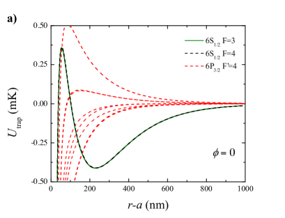
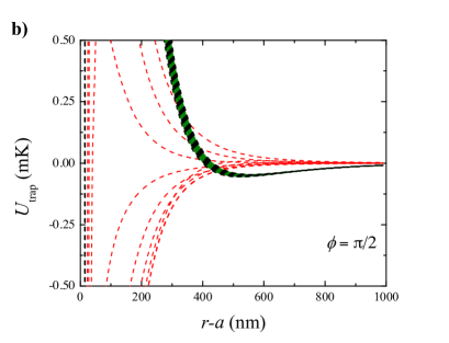
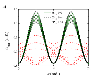
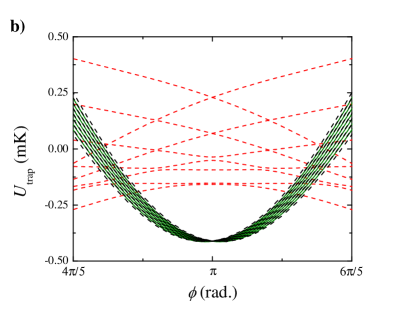
Figure VIIlacroute2012 : Replacement for Fig. 7 in Ref. lacroute2012 . Radial dependence of the trapping potential of the ground and excited states for the parameters used in Ref. vetsch2010 at $z=0$. The polarization configuration is the same as Fig. 1(b) of Ref. lacroute2012 . The energy sublevels of the ground states $F=3$ and $F=4$ of $6S_{1/2}$ are shown as solid green and dashed black curves, and the $F^{\prime}=4$ sublevels of the electronically excited state ($6P_{3/2}$) are shown as red dashed curves. (a) Radial potential along $\phi=0$. The trap minimum is located at about 230 nm from the fiber surface. (b) Radial potential along $\phi=\pi/2$.

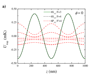
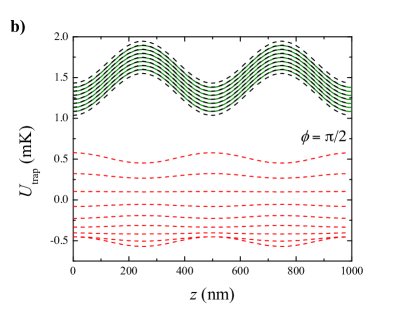
Figure VIIIlacroute2012 : Replacement for Fig. 8 in Ref. lacroute2012 for the configuration of Ref. vetsch2010 . Azimuthal dependence of the trapping potential of the ground and excited states for the parameters used in Fig. IXlacroute2012 . $r-a=230$ nm and $z=0$. (a) The ground-state splitting is minimum for $\phi=0$ and $\phi=\pi$. (b) Expanded view of (a) near a trap minimum at $\phi\simeq\pi$.

Figure IXlacroute2012 : Replacement for Fig. 9 in Ref. lacroute2012 for the configuration of Ref. vetsch2010 . Axial dependence of the trapping potential for the ground and excited states for the parameters used in Fig. IXlacroute2012 . (a) Longitudinal potential along $\phi=0$. The distance from the fiber surface is set to $r-a=230$ nm at the trap minimum. (b) Longitudinal potential along $\phi=\pi/2$. The distance from the fiber surface is again set to 230 nm.

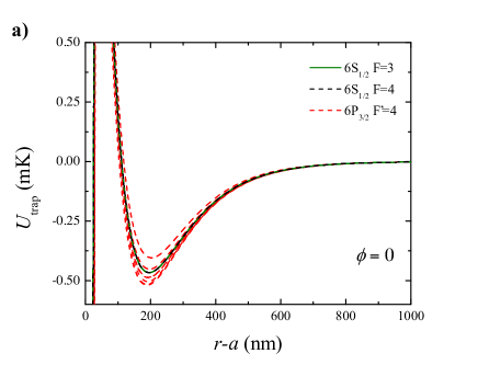
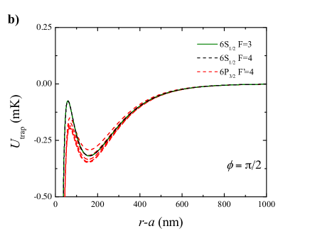
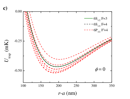
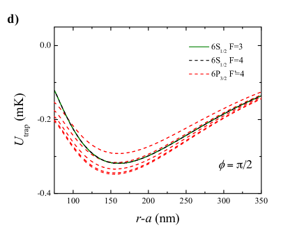
Figure Xlacroute2012 : Replacement for Fig. 10 in Ref. lacroute2012 . Radial dependence of the trapping potentials of the ground and excited states using the magic wavelengths and the compensated configuration shown in Fig. 1(d) of Ref. lacroute2012 . All beams are polarized along $\phi=0$ (i.e., $\varphi_{0}=0$). The 935.3 nm beams each have a power of 0.95 mW. The 684.9 nm beams each have a power of 16 mW. (a) Radial potentials along $\phi=0$ (i.e., $\varphi_{0}=0$). The trap minimum for $6S_{1/2}$ is located at about 200 nm from the fiber surface. (b) Radial potential along $\phi=\pi/2$. (c), (d) Expanded views of (a) and (b) around the trap mininum.

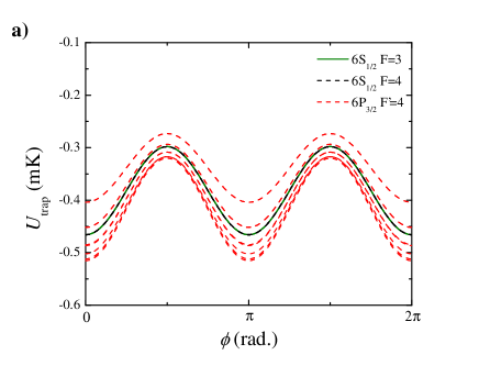
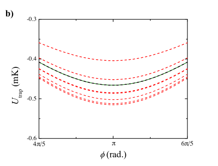
Figure XIlacroute2012 : Replacement for Fig. 11 in Ref. lacroute2012 for the magic, compensated scheme with $\lambda_{\text{red}}=935.3$ nm and $\lambda_{\text{blue}}=684.9$ nm. Azimuthal dependence of the trapping potential of the ground and excited states for the parameters used in Fig. Xlacroute2012 . $r-a=200$ nm and $z=0$. (b) Expanded view of (a) near a trap minimum at $\phi=\pi$.

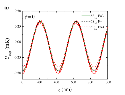
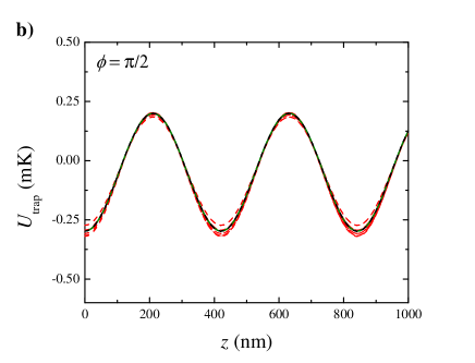
Figure XIIlacroute2012 : Replacement for Fig. 12 in Ref. lacroute2012 for the magic, compensated scheme with $\lambda_{\text{red}}=935.3$ nm and $\lambda_{\text{blue}}=684.9$ nm. Axial dependence of the trapping potential for the ground and excited states for the parameters used in Fig. Xlacroute2012 . (a) Longitudinal potential along $\phi=0$. The distance from the fiber surface is set to $r-a=200$ nm at the trap minimum. (b) Longitudinal potential along $\phi=\pi/2$. The distance from the fiber surface is again set to 200 nm.

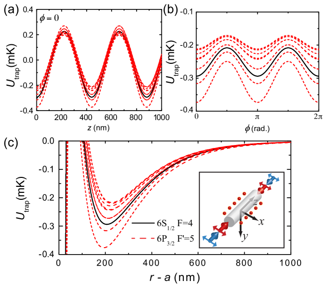
Figure Agoban2012 : The magic, compensated scheme with a pair of counter-propagating $x$-polarized ($\varphi_{0}=0$) red-detuned beams ($P_{\text{red}}=2\times 0.4$ mW) at $\lambda_{\text{red}}=935.7$ nm and counter-propagating, $x$-polarized blue-detuned beams ($P_{\text{blue}}=2\times 5$ mW) at $\lambda_{\text{blue}}=684.8$ nm. The distance from the fiber surface is set to 207 nm. (a) Azimuthal $U_{\rm trap}(\phi)$, (b) axial $U_{\rm trap}(z)$, (c) radial $U_{\rm trap}(r-a)$. Each black and red line corresponds to different energy eigenstates of the ground state ($6S_{1/2},F=4$) and excited state ($6P_{3/2},F^{\prime}=5$), respectively.

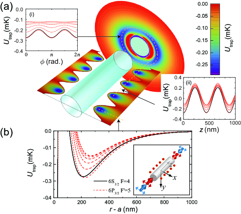
Figure Bgoban2012 : Replacement for Fig. 1 in Ref. goban2012 for the actual wavelengths used in our experiment goban2012 . We used a pair of counter-propagating $x$-polarized ($\varphi_{0}=0$) red-detuned beams ($P_{\text{red}}=2\times 0.4$ mW) at $\lambda_{\text{red}}=937.1$ nm, and counter-propagating, $x$-polarized blue-detuned beams ($P_{\text{blue}}=2\times 5$ mW) at $\lambda_{\text{blue}}=686.1$ nm in our experiment goban2012 . The resulting interference is averaged out by detuning the beams to $\delta_{fb}=382$ GHz. Adiabatic trapping potential $U_{\text{trap}}$ for a state-insensitive, compensated nanofiber trap for the $6S_{1/2},F=4$ states in atomic Cs outside of a cylindrical waveguide of radius $a=215$ nm. $U_{\text{trap}}$ for the substates of the ground level $F=4$ of $6S_{1/2}$ (excited level $F^{\prime}=5$ of $6P_{3/2}$) are shown as black (red-dashed) curves. (a)(i) azimuthal $U_{\text{trap}}(\phi)$, (ii) axial $U_{\text{trap}}(z)$ and (b) radial $U_{\text{trap}}(r-a)$ trapping potentials. The trap minimum for $6S_{1/2}$ is located at about 215 nm from the fiber surface. Input polarizations for the trapping beams are denoted by the red and blue arrows in the inset in (b).

Figure Cgoban2012 : Replacement for Fig. SM5 in the supplemental material of Ref. goban2012 for actual wavelengths used in our experiment goban2012 . We used a pair of counter-propagating $x$-polarized ($\varphi_{0}=0$) red-detuned beams ($P_{\text{red}}=2\times 0.4$ mW) at $\lambda_{\text{red}}=937.1$ nm, and counter-propagating, $x$-polarized blue-detuned beams ($P_{\text{blue}}=2\times 5$ mW) at $\lambda_{\text{blue}}=686.1$ nm in our experiment goban2012 . Expanded view of the insets in Fig. Bgoban2012 . The distance from the fiber surface is set to 215 nm. (a) Azimuthal $U_{\rm trap}(\phi)$, (b) axial $U_{\rm trap}(z)$, (c) radial $U_{\rm trap}(r-a)$. Each black and red line corresponds to different energy eigenstates of the ground state ($6S_{1/2},F=4$) and excited state ($6P_{3/2},F^{\prime}=5$), respectively.

References

• (1) C. Lacroute et al. New J. Phys., 14, 023056 (2012).
• (2) A. Goban et al. Phys. Rev. Lett., 109, 033603 (2012).
• (3) I. H. Deutsch and P. S. Jessen Opt. Comm., 283, 681 (2010).
• (4) D. A. Steck Quantum and Atom Optics textbook.
http://atomoptics.uoregon.edu/ dsteck/teaching/quantum-optics/, 2011.
• (5) P. Rosenbusch et al. Phys. Rev. A, 79, 013404 (2009).
• (6) K. Beloy, PhD Thesis, Theory of the ac Stark Effect on the Atomic Hyper Fine Structure and Applications to Microwave Atomic Clocks, (2009). http://wolfweb.unr.edu/homepage/andrei/WWW-tap/Student_ work/Beloy_ Dissertation_ 2009.pdf
• (7) Fam Le Kien, P. Schneeweiss, and A. Rauschenbeutel arXiv:1211.2673v1 (2012)
• (8) J. McKeever PhD Thesis (2004)
http://thesis.library.caltech.edu/2421, 2004.
In Tables 1 and 2 of this errata, two errors from McKeever’s thesis have been corrected and are highlighted in green, as described in Section II.
• (9) G. Laplanche et al. Phys. Rev. A, 30, 2881 (1984).
• (10) M. Fabry and J. R. Cussenot Can. J. Phys., 54, 836 (1976).
• (11) D. A. Steck Cesium D Line Data
http://steck.us/alkalidata/, 2003.
• (12) C. J. Hood PhD Thesis (2000).
http://thesis.library.caltech.edu/3688.
• (13) B. Arora, M. S. Safronova, C. W. Clark Phys. Rev. A, 76, 052509 (2007).
• (14) J. McKeever et al. Phys. Rev. Lett., 90, 133602 (2003).
• (15) N. P. Stern et al. New J. Phys., 13, 085004(2011).
• (16) E. Vetsch et al. Phys. Rev. Lett., 104, 203603 (2010).