Sign-Error Adaptive Filtering Algorithms for Markovian Parameters

Abstract

Motivated by reduction of computational complexity, this work develops sign-error adaptive filtering algorithms for estimating time-varying system parameters. Different from the previous work on sign-error algorithms, the parameters are time-varying and their dynamics are modeled by a discrete-time Markov chain. A distinctive feature of the algorithms is the multi-time-scale framework for characterizing parameter variations and algorithm updating speeds. This is realized by considering the stepsize of the estimation algorithms and a scaling parameter that defines the transition rates of the Markov jump process. Depending on the relative time scales of these two processes, suitably scaled sequences of the estimates are shown to converge to either an ordinary differential equation, or a set of ordinary differential equations modulated by random switching, or a stochastic differential equation, or stochastic differential equations with random switching. Using weak convergence methods, convergence and rates of convergence of the algorithms are obtained for all these cases.

Key Words. Sign-error algorithms, regime-switching models, stochastic approximation, mean squares errors, convergence, tracking properties.

EDICS. ASP-ANAL

Brief Title. Sign-Error Algorithms for Markovian Parameters

1 Introduction

Adaptive filtering algorithms have been studied extensively, thanks to their simple recursive forms and wide applicability for diversified practical problems arising in estimation, identification, adaptive control, and signal processing [26].

Recent rapid advancement in science and technology has introduced many emerging applications in which adaptive filtering is of substantial utility, including consensus controls, networked systems, and wireless communications; see [1, 2, 4, 5, 8, 7, 12, 13, 14, 16, 17, 18, 19, 20, 23, 24, 27]. One typical scenario of such new domains of applications is that the underlying systems are inherently time varying and their parameter variations are stochastic [29, 30, 31]. One important class of such stochastic systems involves systems whose randomly time-varying parameters can be described by Markov chains. For example, networked systems include communication channels as part of the system topology. Channel connections, interruptions, data transmission queuing and routing, packet delays and losses, are always random. Markov chain models become a natural choice for such systems. For control strategy adaptation and performance optimization, it is essential to capture time-varying system parameters during their operations, which lead to the problems of identifying Markovian regime-switching systems pursued in this paper.

When data acquisition, signal processing, algorithm implementation are subject to resource limitations, it is highly desirable to reduce data complexity. This is especially important when data shuffling involves communication networks. This understanding has motivated the main theme of this paper by using sign-error updating schemes, which carry much reduced data complexity, in adaptive filtering algorithms, without detrimental effects on parameter estimation accuracy and convergence rates.

In our recent work, we developed a sign-regressor algorithm for adaptive filters [28]. The current paper further develops sign-error adaptive filtering algorithms. It is well-known that sign algorithms have the advantage of reduced computational complexity. The sign operator reduces the implementation of the algorithms to bits in data communications and simple bit shifts in multiplications. As such, sign algorithms are highly appealing for practical applications. The work [11] introduced sign algorithms and has inspired much of the subsequent developments in the field. On the other hand, employing sign operators in adaptive algorithms has introduced substantial challenges in establishing convergence properties and error bounds.

A distinctive feature of the algorithms introduced in this paper is the multi-time-scale framework for characterizing parameter variations and algorithm updating speeds. This is realized by considering the stepsize of the estimation algorithms and a scaling parameter that defines the transition rates of the Markov jump process. Depending on the relative time scales of these two processes, suitably scaled sequences of the estimates are shown to converge to either an ordinary differential equation, or a set of ordinary differential equations modulated by random switching, or a stochastic differential equation, or stochastic differential equations with random switching. Using weak convergence methods, convergence and rates of convergence of the algorithms are obtained for all these cases.

The rest of the paper is arranged as follows. Section 2 formulates the problems and introduces the two-time-scale framework. The main algorithms are presented in Section 3. Mean-squares errors on parameter estimators are derived. By taking appropriate continuous-time interpolations, Section 4 establishes convergence properties of interpolated sequences of estimates from the adaptive filtering algorithms. Our analysis is based on weak convergence methods. The convergence properties are obtained by using martingale averaging techniques. Section 5 further investigates the rates of convergence. Suitably interpolated sequences are shown to converge to either stochastic differential equations or randomly-switched stochastic differential equations, depending on relations between the two time scales. Numerical results by simulation are presented to demonstrate the performance of our algorithms in Section 6.

2 Problem Formulation

Let

$$y_{n}=\varphi^{\prime}_{n}\alpha_{n}+e_{n},\ n=0,1,\ldots,$$ (1)

where $\varphi_{n}\in{\mathbb{R}}^{r}$ is the sequence of regression vectors, $e_{n}\in{\mathbb{R}}$ is a sequence of zero mean random variables representing the error or noise, $\alpha_{n}\in{\mathbb{R}}^{r}$ is the time-varying true parameter process, and $y_{n}\in{\mathbb{R}}$ is the sequence of observation signals at time $n$.

Estimates of $\alpha_{n}$ are denoted by $\theta_{n}$ and are given by the following adaptive filtering algorithm using a sign operator on the prediction error

$$\theta_{n+1}=\theta_{n}+\mu\varphi_{n}{\operatorname{sgn}}{(y_{n}-\varphi^{\prime}_{n}\theta_{n})}$$ (2)

where ${\operatorname{sgn}}(y)$ is defined as ${\operatorname{sgn}}(y):=1_{\{y>0\}}-1_{\{y<0\}}$ for $y\in{\mathbb{R}}^{1}$. We impose the following assumptions.

• $\alpha_{n}$ is a discrete-time homogeneous Markov chain with state space

  $${\cal M}=\{a_{1},\ldots,a_{m_{0}}\},\ a_{i}\in{\mathbb{R}}^{r},i=1,\ldots,{m_{0}},$$ (3)

  and whose transition probability matrix is given by

  $$P^{\varepsilon}=I+\varepsilon Q,$$ (4)

  where $\varepsilon>0$ is a small parameter, $I$ is the ${\mathbb{R}}^{{m_{0}}\times{m_{0}}}$ identity matrix, and $Q=(q_{ij})\in{\mathbb{R}}^{{m_{0}}\times{m_{0}}}$ is an irreducible generator (i.e., $Q$ satisfies $q_{ij}\geq 0$ for $i\not=j$ and $\sum^{m_{0}}_{j=1}q_{ij}=0$ for each $i=1,\ldots,{m_{0}}$) of a continuous-time Markov chain. For simplicity, assume that the initial distribution of the Markov chain $\alpha_{n}$ is given by $P(\alpha_{0}=a_{i})=p_{0,i}$, which is independent of $\varepsilon$ for each $i=1,\ldots,{m_{0}}$, where $p_{0,i}\geq 0$ and $\sum^{m_{0}}_{i=1}p_{0,i}=1$.

• The sequence of signals $\{(\varphi_{n},e_{n})\}$ is uniformly bounded, stationary, and independent of the parameter process $\{\alpha_{n}\}$. Let ${\cal F}_{n}$ be the $\sigma$-algebra generated by $\{(\varphi_{j},e_{j}),\alpha_{j}:j<n;\alpha_{n}\}$, and denote the conditional expectation with respect to ${\cal F}_{n}$ by $E_{n}$.

• For each $i=1,\ldots,{m_{0}}$, define

  $$\begin{aligned} &g_{n}:=\varphi_{n}{\operatorname{sgn}}(\varphi^{\prime}_{n}[\alpha_{n}-\theta_{n}]+e_{n})\\ &g_{n}(\theta,i):=\varphi_{n}{\operatorname{sgn}}(\varphi^{\prime}_{n}[a_{i}-\theta]+e_{n})I_{\{\alpha_{n}=a_{i}\}}\\ &\widetilde{g}_{n}(\theta,i):=E_{n}g_{n}(\theta,i)\end{aligned}$$ (5)

  For each $n$ and $i$, there is an $A_{n}^{(i)}\in{\mathbb{R}}^{r\times r}$ such that given $\alpha_{n}=a_{i}$,

  $$\begin{aligned} &\widetilde{g}_{n}(\theta,i)=A^{(i)}_{n}(a_{i}-\theta)I_{\{\alpha_{n}=a_{i}\}}+o(|a_{i}-\theta|I_{\{\alpha_{n}=a_{i}\}})\\ &EA^{(i)}_{n}=A^{(i)}\end{aligned}$$ (6)

• There is a sequence of non-negative real numbers $\{\phi(k)\}$ with $\sum_{k}\phi^{1/2}(k)<\infty$ such that for each $n$ and each $j>n$, and for some $K>0$,

  $$|E_{n}A^{(i)}_{j}-A^{(i)}|\leq K\phi^{1/2}(j-n)$$ (7)

  uniformly in $i=1,\ldots,{m_{0}}$.

Remark 2.1

Let us take a moment to justify the practicality of the assumptions. The boundedness assumption in (A2) is fairly mild. For example, we may use a truncated Gaussian process. In addition, it is possible to accommodate unbounded signals by treating martingale difference sequences (which make the proofs slightly simpler).

In (A3), we consider that while $g_{n}(\theta,i)$ is not smooth w.r.t. $\theta$, its conditional expectation $\widetilde{g}_{n}(\theta,i)$ can be a smooth function of $\theta$. The condition (LABEL:ani) indicates that $\widetilde{g}_{n}(\theta,i)$ is locally (near $a_{i}$) linearizable. For example, this is satisfied if the conditional joint density of $(\varphi_{n},e_{n})$ with respect to $\{\varphi_{j},e_{j},j<n,\varphi_{n}\}$ is differentiable with bounded derivatives; see [6] for more discussion. Finally, (A4) is essentially a mixing condition which indicates that the remote past and distant future are asymptotically independent. Hence we may work with correlated signals as long as the correlation decays sufficiently quickly between iterates.

3 Mean Squares Error Bounds

Denote the sequence of estimation errors by $\widetilde{\theta}_{n}:=\alpha_{n}-\theta_{n}$. We proceed to obtain bounds for the mean squares error in terms of the transition rate of the parameter $\varepsilon$ and the adaptation rate of the algorithm $\mu$.

Theorem 3.1

Assume (A1)–(A4). Then there is an $N_{\varepsilon}>0$ such that for all $n\geq N_{\varepsilon}$,

$$E|\widetilde{\theta}_{n}|^{2}=E|\alpha_{n}-\theta_{n}|^{2}=O\left(\mu+\varepsilon+\varepsilon^{2}/\mu\right).$$ (8)

Proof. Define a function by $V(x)=(x^{\prime}x)/2$. Observe that

$$\widetilde{\theta}_{n+1}=\alpha_{n+1}-\theta_{n+1}=\widetilde{\theta}_{n}-\mu\varphi_{n}{\operatorname{sgn}}(\varphi^{\prime}_{n}\widetilde{\theta}_{n}+e_{n})+(\alpha_{n+1}-\alpha_{n})$$ (9)

so

$$\begin{aligned} E_{n}V(\widetilde{\theta}_{n+1})-V(\widetilde{\theta}_{n})&\!\!\displaystyle=E_{n}\widetilde{\theta}^{\prime}_{n}[(\alpha_{n+1}-\alpha_{n})-\mu\varphi_{n}{\operatorname{sgn}}(\varphi^{\prime}_{n}\widetilde{\theta}_{n}+e_{n})]\\ &\displaystyle\ +E_{n}|(\alpha_{n+1}-\alpha_{n})-\mu\varphi_{n}{\operatorname{sgn}}(\varphi^{\prime}_{n}\widetilde{\theta}_{n}+e_{n})|^{2}\end{aligned}$$ (10)

By (A2), the Markov chain $\alpha_{n}$ is independent of $(\varphi_{n},e_{n})$ and $I_{\{\alpha_{n}=a_{i}\}}$ is ${\cal F}_{n}$-measurable. Since the transition matrix is of the form $P^{\varepsilon}=I+\varepsilon Q$, we obtain

$$\begin{aligned} E_{n}(\alpha_{n+1}-\alpha_{n})&\!\!\displaystyle=\sum^{m_{0}}_{i=1}E(\alpha_{n+1}-a_{i}\Big{|}\alpha_{n}=a_{i})I_{\{\alpha_{n}=a_{i}\}}\\ &\!\!\displaystyle=\sum^{m_{0}}_{i=1}\Big{[}\sum^{m_{0}}_{j=1}a_{j}(\delta_{ij}+\varepsilon q_{ij})-a_{i}\Big{]}I_{\{\alpha_{n}=a_{i}\}}=O(\varepsilon)\end{aligned}$$ (11)

Similarly,

$$\begin{aligned} E_{n}|\alpha_{n+1}-\alpha_{n}|^{2}&\!\!\displaystyle=\sum^{m_{0}}_{j=1}\sum^{m_{0}}_{i=1}|a_{j}-a_{i}|^{2}I_{\{\alpha_{n}=a_{i}\}}P(\alpha_{n+1}=a_{j}|\alpha_{n}=a_{i})\\ &\!\!\displaystyle=\sum^{m_{0}}_{j=1}\sum^{m_{0}}_{i=1}|a_{j}-a_{i}|^{2}I_{\{\alpha_{n}=a_{i}\}}(\delta_{ij}+\varepsilon q_{ij})\\ &\!\!\displaystyle=O(\varepsilon)\end{aligned}$$ (12)

Note that $|\widetilde{\theta}_{n}|=|\widetilde{\theta}_{n}|\cdot 1\leq(|\widetilde{\theta}_{n}|^{2}+1)/2$, so

$$O(\varepsilon)|\widetilde{\theta}_{n}|\leq O(\varepsilon)(V(\widetilde{\theta}_{n})+1).$$ (13)

Since the signals $\{(\varphi_{n},e_{n})\}$ are bounded, we have

$$\begin{aligned} &\!\!\displaystyle E_{n}|(\alpha_{n+1}-\alpha_{n})-\mu\varphi_{n}{\operatorname{sgn}}(\varphi^{\prime}_{n}\widetilde{\theta}_{n}+e_{n})|^{2}\\ &\displaystyle\ =E_{n}|\alpha_{n+1}-\alpha_{n}|^{2}+O(\mu^{2}+\mu\varepsilon)[V(\widetilde{\theta}_{n})+1)\end{aligned}$$ (14)

Applying (LABEL:thesa) to (10), we arrive at

$$\begin{aligned} &\!\!\displaystyle E_{n}V(\widetilde{\theta}_{n+1})-V(\widetilde{\theta}_{n})=-\mu E_{n}\widetilde{\theta}^{\prime}_{n}\varphi_{n}{\operatorname{sgn}}(\varphi^{\prime}_{n}\widetilde{\theta}_{n}+e_{n})+E_{n}\widetilde{\theta}^{\prime}_{n}(\alpha_{n+1}-\alpha_{n})\\ &\displaystyle\quad+E_{n}|\alpha_{n+1}-\alpha_{n}|^{2}+O(\mu^{2}+\mu\varepsilon)[V(\widetilde{\theta}_{n})+1]\end{aligned}$$ (15)

Note also that by (A3),

$$\begin{aligned} \mu E_{n}\widetilde{\theta}^{\prime}_{n}\varphi_{n}{\operatorname{sgn}}(\varphi^{\prime}_{n}\widetilde{\theta}_{n}+e_{n})&\!\!\displaystyle=\mu\sum^{m_{0}}_{i=1}E_{n}\widetilde{\theta}^{\prime}_{n}\varphi_{n}{\operatorname{sgn}}(\varphi^{\prime}_{n}\widetilde{\theta}_{n}+e_{n})I_{\{\alpha_{n}=a_{i}\}}\\ &\!\!\displaystyle=\mu\sum^{m_{0}}_{i=1}E_{n}\widetilde{\theta}^{\prime}_{n}A^{(i)}_{n}\widetilde{\theta}_{n}I_{\{\alpha_{n}=a_{i}\}}+\mu o(\widetilde{\theta}_{n})\\ &\!\!\displaystyle=\mu\sum^{m_{0}}_{i=1}\widetilde{\theta}^{\prime}_{n}[A^{(i)}_{n}-A^{(i)}]\widetilde{\theta}_{n}I_{\{\alpha_{n}=a_{i}\}}+\mu\sum^{m_{0}}_{i=1}\widetilde{\theta}^{\prime}_{n}A^{(i)}\widetilde{\theta}_{n}I_{\{\alpha_{n}=a_{i}\}}+\mu o(\widetilde{\theta}_{n})\end{aligned}$$ (16)

To treat the first three terms in (LABEL:v-0a), we define the following perturbed Liapunov functions by

$$\begin{aligned} &V^{\mu}_{1}(\widetilde{\theta},n):=\sum^{\infty}_{j=n}\sum^{m_{0}}_{i=1}-\mu E_{n}\widetilde{\theta}^{\prime}[A^{(i)}_{j}-A^{(i)}]\widetilde{\theta}I_{\{\alpha_{j}=a_{i}\}}\\ &V^{\mu}_{2}(\widetilde{\theta},n):=\sum^{\infty}_{j=n}\widetilde{\theta}^{\prime}E_{n}(\alpha_{j+1}-\alpha_{j})\\ &V^{\mu}_{3}(n):=\sum_{j=n}^{\infty}E_{n}(\alpha_{n+1}-\alpha_{n})^{\prime}(\alpha_{j+1}-\alpha_{j})\end{aligned}$$ (17)

By virtue of (A4), we have

$$\begin{aligned} |V^{\mu}_{1}(\widetilde{\theta},n)|\leq\mu\sum^{m_{0}}_{i=1}K|\widetilde{\theta}|^{2}\sum^{\infty}_{j=n}\phi^{1/2}(j-n)\leq O(\mu)[V(\widetilde{\theta})+1]\end{aligned}$$ (18)

Note also that the irreducibility of $Q$ implies that of $I+\varepsilon Q$ for sufficiently small $\varepsilon>0$. Thus there is an $N_{\varepsilon}$ such that for all $n\geq N_{\varepsilon}$, $|(I+\varepsilon Q)^{k}-{\rm 1}{\rm l}\nu_{\varepsilon}|\leq\lambda_{c}^{k}$ for some $0<\lambda_{c}<1$, where $\nu_{\varepsilon}$ denotes the stationary distribution associated with the transition matrix $I+\varepsilon Q$. Note that the difference of the $j+1-n$ and $j-n$ step transition matrices is given by

$$\begin{array}[]{rl}&\!\!\displaystyle(I+\varepsilon Q)^{j+1-n}-(I+\varepsilon Q)^{j-n}\\ &\displaystyle\ =[(I+\varepsilon Q)-I](I+\varepsilon Q)^{j-n}\\ &\displaystyle\ =[(I+\varepsilon Q)-I][(I+\varepsilon Q)^{j-n}-{\rm 1}{\rm l}\nu_{\varepsilon}]+[(I+\varepsilon Q)-I]{\rm 1}{\rm l}\nu_{\varepsilon}\\ &\displaystyle\ =(\varepsilon Q)[(I+\varepsilon Q)^{j-n}-{\rm 1}{\rm l}\nu_{\varepsilon}].\end{array}$$

The last line above follows from the fact $Q{\rm 1}{\rm l}=0$, hence $[(I+\varepsilon Q)-I]{\rm 1}{\rm l}\nu_{\varepsilon}=0$. Thus

$$\sum^{\infty}_{j=n}|I+\varepsilon Q)^{j+1-n}-(I+\varepsilon Q)^{j-n}|\leq O(\varepsilon)\sum^{\infty}_{j=n}\lambda^{j-n}_{c}=O(\varepsilon).$$ (19)

The forgoing estimates lead to $\sum^{\infty}_{j=n}E_{n}(\alpha_{j+1}-\alpha_{j})=O(\varepsilon)$ and as a result

$$|V^{\mu}_{2}(\widetilde{\theta},n)|\leq O(\varepsilon)(V(\widetilde{\theta})+1).$$ (20)

and similarly

$$|V^{\mu}_{3}(n)|=O(\varepsilon),$$ (21)

so all the perturbations can be made small.

Now, we note that

$$\begin{aligned} &E_{n}V^{\mu}_{1}(\widetilde{\theta}_{n+1},n+1)-V^{\mu}_{1}(\widetilde{\theta}_{n},n)\\ &=E_{n}V^{\mu}_{1}(\widetilde{\theta}_{n+1},n+1)-E_{n}V^{\mu}_{1}(\widetilde{\theta}_{n},n+1)+E_{n}V^{\mu}_{1}(\widetilde{\theta}_{n},n+1)-V^{\mu}_{n}(\widetilde{\theta}_{n},n).\end{aligned}$$ (22)

where

$$E_{n}V^{\mu}_{1}(\widetilde{\theta}_{n},n+1)-V^{\mu}_{1}(\widetilde{\theta}_{n},n)=\mu\sum^{m_{0}}_{i=1}\widetilde{\theta}^{\prime}_{n}[A^{(i)}_{n}-A^{(i)}]\widetilde{\theta}_{n}I_{\{\alpha_{n}=a_{i}\}}$$ (23)

and

$$\begin{aligned} &\!\!\displaystyle E_{n}V^{\mu}_{1}(\widetilde{\theta}_{n+1},n+1)-E_{n}V^{\mu}_{1}(\widetilde{\theta}_{n},n+1)\\ &\displaystyle\ =\mu\sum^{\infty}_{j=n+1}\sum^{m_{0}}_{i=1}E_{n}(\widetilde{\theta}_{n+1}-\widetilde{\theta}_{n})^{\prime}[A^{(i)}_{j}-A^{(i)}]\widetilde{\theta}_{n+1}I_{\{\alpha_{n}=a_{i}\}}\\ &\displaystyle\quad+\mu\sum^{\infty}_{j=n+1}\sum^{m_{0}}_{i=1}E_{n}\widetilde{\theta}_{n}^{\prime}[A^{(i)}_{j}-A^{(i)}](\widetilde{\theta}_{n+1}-\widetilde{\theta}_{n})I_{\{\alpha_{n}=a_{i}\}}.\end{aligned}$$ (24)

Using (11), we have

$$\begin{aligned} &E_{n}|\widetilde{\theta}_{n+1}-\widetilde{\theta}_{n}|\leq E_{n}|\alpha_{n+1}-\alpha_{n}|+\mu E_{n}|\varphi_{n}{\operatorname{sgn}}(\varphi^{\prime}_{n}\widetilde{\theta}_{n}+e_{n})|=O(\varepsilon+\mu).\end{aligned}$$ (25)

Thus, in view of (A4)

$$\begin{aligned} &\left|\mu\sum^{\infty}_{j=n+1}\sum^{m_{0}}_{i=1}E_{n}\widetilde{\theta}_{n}^{\prime}E_{n+1}[A^{(i)}_{j}-A^{(i)}](\widetilde{\theta}_{n+1}-\widetilde{\theta}_{n})I_{\{\alpha_{n}=a_{i}\}}\right|\leq O(\mu^{2}+\mu\varepsilon)[V(\widetilde{\theta}_{n})+1],\end{aligned}$$ (26)

and

$$\begin{aligned} \left|\mu\sum^{\infty}_{j=n+1}\sum^{m_{0}}_{i=1}E_{n}(\widetilde{\theta}_{n+1}-\widetilde{\theta}_{n})^{\prime}E_{n+1}[A^{(i)}_{j}-A^{(i)}]\widetilde{\theta}_{n+1}I_{\{\alpha_{n}=a_{i}\}}\right|\leq O(\mu^{2}+\mu\varepsilon)[V(\widetilde{\theta}_{n})+1].\end{aligned}$$ (27)

Putting together (LABEL:v1-est00)–(27), we establish that

$$\begin{aligned} &E_{n}V^{\mu}_{1}(\widetilde{\theta}_{n+1},n+1)-V^{\mu}_{1}(\widetilde{\theta}_{n},n)=\mu\sum^{m_{0}}_{i=1}E_{n}\widetilde{\theta}^{\prime}_{n}[A^{(i)}_{j}-A^{(i)}]\widetilde{\theta}_{n}I_{\{\alpha_{n}=a_{i}\}}+O(\mu^{2}+\mu\varepsilon)[V(\widetilde{\theta}_{n})+1].\end{aligned}$$ (28)

Likewise, we can obtain

$$\begin{aligned} E_{n}V^{\mu}_{2}(\widetilde{\theta}_{n+1},n+1)-V^{\mu}_{2}(\widetilde{\theta}_{n},n)=-E_{n}\widetilde{\theta}^{\prime}_{n}(\alpha_{n+1}-\alpha_{n})+O(\varepsilon^{2}+\mu^{2})\end{aligned}$$ (29)

and

$$\begin{aligned} E_{n}V^{\mu}_{3}(n+1)-V^{\mu}_{3}(n)=-E_{n}|\alpha_{n+1}-\alpha_{n}|^{2}+O(\varepsilon^{2}).\end{aligned}$$ (30)

Now we define

$$W(\widetilde{\theta},n)=V(\widetilde{\theta})+V^{\mu}_{1}(\widetilde{\theta},n)+V^{\mu}_{2}(\widetilde{\theta},n)+V^{\mu}_{3}(n).$$

Since each $A^{(i)}$ is a stable matrix there is a $\lambda>0$ such that $\widetilde{\theta}^{\prime}A^{(i)}\widetilde{\theta}\geq\lambda V(\widetilde{\theta})$ for each $i$. Thus we may take $\lambda$ such that $-\mu\sum^{m_{0}}_{i=1}\widetilde{\theta}^{\prime}A^{(i)}\widetilde{\theta}I_{\{\alpha_{n}=a_{i}\}}-\mu O(\widetilde{\theta})\leq-\lambda\mu V(\widetilde{\theta})$. Using this along with (10), (16), (LABEL:v1-est-fin)–(30), and the inequality $O(\mu\varepsilon)=O(\mu^{2}+\varepsilon^{2})$, we arrive at

$$\begin{aligned} &E_{n}W(\widetilde{\theta}_{n+1},n+1)-W(\widetilde{\theta}_{n},n)\\ &\qquad=-\mu\sum^{m_{0}}_{i=1}\widetilde{\theta}^{\prime}_{n}A^{(i)}\widetilde{\theta}_{n}I_{\{\alpha_{n}=a_{i}\}}-\mu O(\widetilde{\theta}_{n})+O(\mu^{2}+\varepsilon^{2})[V(\widetilde{\theta}_{n})+1]\\ &\qquad\leq-\lambda\mu V(\widetilde{\theta}_{n})+O(\mu^{2}+\varepsilon^{2})[V(\widetilde{\theta}_{n})+1]\\ &\qquad\leq-\lambda\mu W(\widetilde{\theta}_{n},n)+O(\mu^{2}+\varepsilon^{2})[W(\widetilde{\theta}_{n},n)+1].\end{aligned}$$ (31)

Choose $\mu$ and $\varepsilon$ small enough so that there is a $\lambda_{0}>0$ satisfying $\lambda_{0}\leq\lambda$ and

$$-\lambda\mu+O(\mu^{2})+O(\varepsilon^{2})\leq-\lambda_{0}\mu.$$

Then we obtain

$$E_{n}W(\widetilde{\theta}_{n+1},n+1)\leq(1-\lambda_{0}\mu)W(\widetilde{\theta}_{n},n)+O(\mu^{2}+\varepsilon^{2}).$$

Note that there is an $N_{\varepsilon}>0$ such that $(1-\lambda_{0}\mu)^{n}\leq O(\mu)$ for $n\geq N_{\varepsilon}$. Taking expectation in the iteration for $W(\widetilde{\theta}_{n},n)$ and iterating on the resulting inequality yield

$$\begin{array}[]{rl}&\!\!\displaystyle EW(\widetilde{\theta}_{n+1},n+1)\leq(1-\lambda_{0}\mu)^{n}W(\widetilde{\theta}_{0},0)+O\left(\mu+\varepsilon^{2}/\mu\right).\end{array}$$

Thus

$$EW(\widetilde{\theta}_{n+1},n+1)\leq O(\mu+\varepsilon^{2}/\mu).$$

Finally, applying (18)–(21) again, we also obtain

$$EV(\widetilde{\theta}_{n+1})\leq O(\mu+\varepsilon+\varepsilon^{2}/\mu).$$

Thus the desired result follows. $\Box$

4 Convergence Properties

4.1 Switching ODE Limit: $\mu=O(\varepsilon)$

We assume the adaptation rate and the transition frequency are of the same order, that is $\mu=O(\varepsilon)$. For simplicity, we take $\mu=\varepsilon$. To study the asymptotic properties of the sequence $\{\theta_{n}\}$, we take a continuous-time interpolation of the process. Define

$$\theta^{\mu}(t)=\theta_{n},\ \alpha^{\mu}(t)=\alpha_{n},\ \hbox{ for }\ t\in[n\mu,n\mu+\mu).$$

We proceed to prove that $\theta^{\mu}(\cdot)$ converges weakly to a system of randomly switching ordinary differential equations.

Theorem 4.1

Assume (A1)–(A4) hold and $\varepsilon=\mu$. Then the process $(\theta^{\mu}(\cdot),\alpha^{\mu}(\cdot))$ converges weakly to $(\theta(\cdot),\alpha(\cdot))$ such that $\alpha(\cdot)$ is a continuous-time Markov chain generated by $Q$ and the limit process $\theta(\cdot)$ satisfies the Markov switched ordinary differential equation

$$\dot{\theta}(t)=A^{(\alpha(t))}(\alpha(t)-\theta(t)),\ \theta(0)=\theta_{0}.$$ (32)

The theorem is established through a series of lemmas. We begin by using a truncation device to bound the estimates. Define $S_{N}=\{\theta\in{\mathbb{R}}^{r}:|\theta|\leq N\}$ to be the ball with radius $N$, and $q^{N}(\cdot)$ as a truncation function that is equal to 1 for $\theta\in S_{N}$, 0 for $\theta\in S_{N+1}$, and sufficiently smooth between. Then we modify algorithm (2) so that

$$\theta^{N}_{n+1}:=\theta^{N}_{n}+\mu\varphi_{n}{\operatorname{sgn}}(y_{n}-\varphi^{\prime}_{n}\theta^{N}_{n})q^{N}(\theta^{N}_{n}),\ n=0,1,\ldots,$$ (33)

is now a bounded sequence of estimates. As before, define

$$\theta^{N,\mu}(t):=\theta^{N}_{n}\ \hbox{ for }\ t\in[\mu n,\mu n+\mu).$$

We shall first show that the sequence $\{\theta^{N,\mu}(\cdot),\alpha^{\mu}(\cdot)\}$ is tight, and thus by Prohorov’s theorem we may extract a convergent subsequence. We will then show the limit satisfies a switched differential equation. Lastly, we let the truncation bound $N$ grow and show the untruncated sequence given by (2) is also weakly convergent.

Lemma 4.2

The sequence $(\theta^{N,\mu}(\cdot),\alpha^{\mu}(\cdot))$ is tight in $D([0,\infty):{\mathbb{R}}^{r}\times{\cal M})$.

Proof of Lemma 4.2. Note that the sequence $\alpha^{\mu}(\cdot)$ is tight by virtue of [33, Theorem 4.3]. In addition, $\alpha^{\mu}(\cdot)$ converges weakly to a Markov chain generated by $Q$. To proceed, we examine the asymptotics of the sequence $\theta^{N,\mu}(\cdot)$. We have that for any $\delta>0$, and $t,s>0$ satisfying $s\leq\delta$,

$$\begin{aligned} &\!\!\!E^{\mu}_{t}\left|\theta^{N,\mu}(t+s)-\theta^{N,\mu}(t)\right|^{2}\leq E^{\mu}_{t}\left|\mu\sum^{(t+s)/\mu-1}_{k=t/\mu}\varphi_{k}{\operatorname{sgn}}(y_{k}-\varphi^{\prime}_{k}\theta^{N}_{k})q^{N}(\theta^{N}_{k})\right|^{2}\\ &\leq\mu^{2}E^{\mu}_{t}\sum^{(t+s)/\mu-1}_{j=t/\mu}\sum^{(t+s)/\mu-1}_{k=t/\mu}\varphi^{\prime}_{j}\varphi_{k}{\operatorname{sgn}}(y_{j}-\varphi^{\prime}_{j}\theta^{N}_{j}){\operatorname{sgn}}(y_{k}-\varphi^{\prime}_{k}\theta^{N}_{k})q^{N}(\theta^{N}_{j})q^{N}(\theta^{N}_{k})\\ &\leq\mu^{2}\sum^{(t+s)/\mu-1}_{j=t/\mu}\sum^{(t+s)/\mu-1}_{k=t/\mu}E^{\mu}_{t}\left|\varphi_{j}\right|^{2}E^{\mu}_{t}\left|\varphi_{k}\right|^{2}\leq O(s^{2})\leq O(\delta^{2}).\end{aligned}$$ (34)

For any $T<\infty$ and any $0\leq t\leq T$, use $E^{\mu}_{t}$ to denote the conditional expectation w.r.t. the $\sigma$-algebra ${\cal F}^{\mu}_{t}$, we have

$$\lim_{\delta\to 0}\limsup_{\mu\to 0}\Big{\{}\sup_{0\leq s\leq\delta}E[E^{\mu}_{t}\left|\theta^{N,\mu}(t+s)-\theta^{N,\mu}(t)\right|^{2}]\Big{\}}=0.$$

Applying the criterion [15, p.47], the tightness is proved. $\Box$

Since $(\theta^{N,\mu}(\cdot),\alpha^{\mu}(\cdot))$ is tight, it is sequentially compact. By virtue of Prohorov’s theorem, we can extract a weakly convergence subsequence. Select such a subsequence and still denote it by $(\theta^{N,\mu}(\cdot),\alpha^{\mu}(\cdot))$ for notational simplicity. Denote the limit by $(\theta^{N}(\cdot),\alpha(\cdot))$. We proceed to characterize the limit process.

Lemma 4.3

The sequence $(\theta^{N,\mu}(\cdot),\alpha^{\mu}(\cdot))$ converges weakly to $(\theta^{N}(\cdot),\alpha(\cdot))$ that is a solution of the martingale problem with operator

$$L_{1}^{N}f(\theta^{N},a_{i}):=\nabla f^{\prime}(\theta^{N},a_{i})A^{(i)}[a_{i}-\theta^{N}]q^{N}(\theta^{N})+\sum^{m_{0}}_{j=1}q_{ij}f(\theta^{N},a_{j}),$$ (35)

where for each $i\in{\cal M}$, $f(\cdot,i)\in C^{1}_{0}$ $(C^{1}$ functions with compact support$)$.

Proof. To derive the martingale limit, we need only show that for the $C^{1}$ function with compact support $f(\cdot,i)$, for each bounded and continuous function $h(\cdot)$, each $t,s>0$, each positive integer $\kappa$, and each $t_{i}\leq t$ for $i\leq\kappa$,

$$\begin{aligned} \displaystyle Eh(\theta^{N}(t_{i}),\alpha(t_{i}):i\leq\kappa)&\Big{[}f(\theta^{N}(t+s),\alpha(t+s))-f(\theta^{N}(t),\alpha(t))\\ &\quad-\int^{t+s}_{t}L_{1}^{N}f(\theta^{N}(\tau),\alpha(\tau))d\tau\Big{]}=0.\end{aligned}$$ (36)

To verify (36), we use the processes indexed by $\mu$. As before, note that

$$\begin{aligned} \theta^{N,\mu}(t+s)-\theta^{N,\mu}(t)=\sum^{(t+s)/\mu-1}_{k=t/\mu}\mu\varphi_{k}{\operatorname{sgn}}(\varphi^{\prime}_{k}[\alpha_{k}-\theta_{k}]+e_{k})q^{N}(\theta^{N}_{k}).\end{aligned}$$ (37)

Subdivide the interval with the end points $t/\mu$ and $(t+s)/\mu-1$ by choosing $m_{\mu}$ such that $m_{\mu}\to\infty$ as $\mu\to 0$ but $\delta_{\mu}=\mu m_{\mu}\to 0$. By the smoothness of $f(\cdot,i)$, it is readily seen that as $\mu\to 0$,

$$\begin{aligned} &\!\!\!Eh(\theta^{N,\mu}(t_{i}),\alpha^{\mu}(t_{i}):i\leq\kappa)\left[f(\theta^{N,\mu}(t+s),\alpha^{\mu}(t+s))-f(\theta^{N,\mu}(t),\alpha^{\mu}(t))\right]\\ &\to Eh(\theta^{N}(t_{i}),\alpha(t_{i}):i\leq\kappa)\left[f(\theta^{N}(t+s),\alpha(t+s))-f(\theta^{N}(t),\alpha(t))\right].\end{aligned}$$ (38)

Next, we insert a term to examine the change in the parameter $\alpha$ and the estimate $\theta^{N}$ separately

$$\begin{aligned} &\!\!\!\lim_{\mu\to 0}Eh(\theta^{N,\mu}(t_{i}),\alpha^{\mu}(t_{i}):i\leq\kappa)\left[f(\theta^{N,\mu}(t+s),\alpha^{\mu}(t+s))-f(\theta^{N,\mu}(t),\alpha^{\mu}(t))\right]\\ &\ =\lim_{\mu\to 0}Eh(\theta^{N,\mu}(t_{i}),\alpha^{\mu}(t_{i}):i\leq\kappa)\left[\sum^{t+s}_{l\delta_{\mu}=t}[f(\theta^{N}_{lm_{\mu}+m_{\mu}},\alpha_{lm_{\mu}+m_{\mu}})-f(\theta^{N}_{lm_{\mu}},\alpha_{lm_{\mu}})]\right]\\ &\ =\lim_{\mu\to 0}Eh(\theta^{N,\mu}(t_{i}),\alpha^{\mu}(t_{i}):i\leq\kappa)\Big{[}\sum^{t+s}_{l\delta_{\mu}=t}[f(\theta^{N}_{lm_{\mu}+m_{\mu}},\alpha_{lm_{\mu}+m_{\mu}})-f(\theta^{N}_{lm_{\mu}+m_{\mu}},\alpha_{lm_{\mu}})]\\ &\hskip 86.72377pt+\sum^{t+s}_{l\delta_{\mu}=t}[f(\theta^{N}_{lm_{\mu}+m_{\mu}},\alpha_{lm_{\mu}})-f(\theta^{N}_{lm_{\mu}},\alpha_{lm_{\mu}})]\Big{]}.\end{aligned}$$ (39)

First, we work with the last term in (LABEL:w-es2). By using a Taylor expansion on each interval indexed by $l$ we have

$$\begin{aligned} &\!\!\!\lim_{\mu\to 0}Eh(\theta^{N,\mu}(t_{i}),\alpha^{\mu}(t_{i}):i\leq\kappa)\Big{[}\sum^{t+s}_{l\delta_{\mu}=t}[f(\theta^{N}_{lm_{\mu}+m_{\mu}},\alpha_{lm_{\mu}})-f(\theta^{N}_{lm_{\mu}},\alpha_{lm_{\mu}})]\Big{]}\\ &=\lim_{\mu\to 0}Eh(\theta^{N,\mu}(t_{i}),\alpha^{\mu}(t_{i}):i\leq\kappa)\sum^{t+s}_{l\delta_{\mu}=t}\Big{[}\delta_{\mu}{1\over m_{\mu}}\sum^{lm_{\mu}+m_{\mu}-1}_{k=lm_{\mu}}\nabla f^{\prime}(\theta^{N}_{lm_{\mu}},\alpha_{lm_{\mu}})\\ &\qquad\quad\hfill\times\varphi_{k}{\operatorname{sgn}}(\varphi^{\prime}_{k}(\alpha_{k}-\theta^{N}_{k})+e_{k})q^{N}(\theta^{N}_{k})\\ &\qquad\qquad\qquad\qquad+\sum^{lm_{\mu}+\mu-1}_{k=lm_{\mu}}[\nabla f^{\prime}(\theta^{N,+}_{lm_{\mu}},\alpha_{lm\mu})-\nabla f^{\prime}(\theta^{N}_{lm_{\mu}},\alpha_{lm\mu})](\theta^{N}_{k+1}-\theta^{N}_{k})q^{N}(\theta^{N}_{k})\Big{]}.\end{aligned}$$ (40)

where $\theta^{N,+}_{lm_{\mu}}$ is a point on the line segment joining $\theta^{N}_{lm_{\mu}}$ and $\theta^{N}_{lm_{\mu}+m_{\mu}}$. Since

$$|\theta^{N}_{lm_{\mu}+m_{\mu}}-\theta^{N}_{lm_{\mu}}|=O(\delta_{\mu})$$

and $\nabla f^{\prime}(\cdot,i)$ is smooth, we have the last term in (LABEL:ode0) is $o(1)$ in the sense of in probability as $\mu\to 0$. To work with the first term we insert the conditional expectation $E_{k}$ and apply (LABEL:ani) to obtain

$$\begin{aligned} &\lim_{\mu\to 0}Eh(\theta^{N,\mu}(t_{i}),\alpha^{\mu}(t_{i}):i\leq\kappa)\sum^{t+s}_{l\delta_{\mu}=t}\delta_{\mu}{1\over m_{\mu}}\sum^{lm_{\mu}+m_{\mu}-1}_{k=lm_{\mu}}\nabla f^{\prime}(\theta^{N}_{lm_{\mu}},\alpha_{lm_{\mu}})\\ &\qquad\qquad\times E_{k}[\varphi^{\prime}_{k}{\operatorname{sgn}}(\varphi^{\prime}_{k}(\alpha_{k}-\theta^{N}_{k})+e_{k})]q^{N}(\theta^{N}_{k})\\ &=\lim_{\mu\to 0}Eh(\theta^{N,\mu}(t_{i}),\alpha^{\mu}(t_{i}):i\leq\kappa)\sum^{t+s}_{l\delta_{\mu}=t}\sum^{m_{0}}_{j=1}\delta_{\mu}{1\over m_{\mu}}\sum^{lm_{\mu}+m_{\mu}-1}_{k=lm_{\mu}}\nabla f^{\prime}(\theta^{N}_{lm_{\mu}},\alpha_{lm_{\mu}})\\ &\qquad\qquad\times\Big{[}A_{k}^{(j)}(a_{j}-\theta^{N}_{k})+o(|\alpha_{k}-\theta^{N}_{k}|)\Big{]}q^{N}(\theta^{N}_{k})I_{\{\alpha_{k}=a_{j}\}}.\end{aligned}$$ (41)

Then for small $\mu$,

$$E{1\over m_{\mu}}\sum^{lm_{\mu}+m_{\mu}-1}_{k=lm_{\mu}}\nabla f^{\prime}(\theta^{N}_{lm_{\mu}},\alpha_{lm_{\mu}})o(|\alpha_{k}-\theta^{N}_{k}|)\leq KE|\alpha_{lm_{\mu}}-\theta_{lm_{\mu}}|=O(\mu^{1/2}).$$ (42)

Letting $\mu lm_{\mu}\to\tau$, then by (7),

$$\begin{aligned} &\!\!\!\lim_{\mu\to 0}Eh(\theta^{N,\mu}(t_{i}),\alpha^{\mu}(t_{i}):i\leq\kappa)\sum^{t+s}_{l\delta_{\mu}=t}\sum^{m_{0}}_{j=1}{\delta_{\mu}\over m_{\mu}}\sum^{lm_{\mu}+m_{\mu}-1}_{k=lm_{\mu}}\nabla f^{\prime}(\theta^{N}_{lm_{\mu}},\alpha_{lm_{\mu}})A_{k}^{(j)}(a_{j}-\theta^{N}_{k})\\ &\qquad\qquad\times q^{N}(\theta^{N}_{k})I_{\{\alpha_{k}=a_{j}\}}\\ &=\lim_{\mu\to 0}Eh(\theta^{N,\mu}(t_{i}),\alpha^{\mu}(t_{i}):i\leq\kappa)\sum^{t+s}_{l\delta_{\mu}=t}\sum^{m_{0}}_{j=1}{\delta_{\mu}\over m_{\mu}}\sum^{lm_{\mu}+m_{\mu}-1}_{k=lm_{\mu}}\nabla f^{\prime}(\theta^{N}_{lm_{\mu}},\alpha_{lm_{\mu}})\Big{[}A^{(j)}(a_{j}-\theta^{N}_{k})\\ &\hskip 252.94499pt+[A_{k}^{(j)}-A^{(j)}](a_{j}-\theta^{N}_{k})\Big{]}q^{N}(\theta^{N}_{k})I_{\{\alpha_{k}=a_{j}\}}\\ &=\lim_{\mu\to 0}Eh(\theta^{N,\mu}(t_{i}),\alpha^{\mu}(t_{i}):i\leq\kappa)\sum^{t+s}_{l\delta_{\mu}=t}\sum^{m_{0}}_{j=1}\delta_{\mu}\nabla f^{\prime}(\theta^{N}_{lm_{\mu}},\alpha_{lm_{\mu}}){1\over m_{\mu}}\sum^{lm_{\mu}+m_{\mu}-1}_{k=lm_{\mu}}A^{(j)}(a_{j}-\theta^{N}_{k})\\ &\qquad\qquad\times q^{N}(\theta^{N}_{k})I_{\{\alpha_{k}=a_{j}\}}\\ &=Eh(\theta^{N}(t_{i}),\alpha(t_{i}):i\leq\kappa)\int^{t+s}_{t}\nabla f^{\prime}(\theta^{N}(\tau),\alpha(\tau))A^{(\alpha(\tau))}[\alpha(\tau)-\theta^{N}(\tau)]q^{N}(\tau)d\tau.\end{aligned}$$ (43)

Likewise, we can obtain

$$\begin{array}[]{ll}&\!\!\displaystyle\lim_{\mu\to 0}Eh(\theta^{N,\mu}(t_{i}),\alpha^{\mu}(t_{i}):i\leq\kappa)\sum^{t+s}_{l\delta_{\mu}=t}[f(\theta^{N}_{lm_{\mu}+m_{\mu}},\alpha_{lm_{\mu}+m_{\mu}})-f(\theta^{N}_{lm_{\mu}+m_{\mu}},\alpha_{lm_{\mu}})]\\ &\displaystyle\ =Eh(\theta^{N,\mu}(t_{i}),\alpha^{\mu}(t_{i}):i\leq\kappa)\sum^{lm_{\mu}+m_{\mu}-1}_{k=lm_{\mu}}[f(\alpha^{N}_{lm_{\mu}},\alpha_{lm_{\mu}+m_{\mu}})-f(\theta^{N}_{lm_{\mu}},\alpha_{lm_{\mu}})]\\ &\displaystyle\ =Eh(\theta^{N}(t_{i}),\alpha(t_{i}):i\leq\kappa)\left[\int^{t+s}_{t}Qf(\theta^{N}(\tau),\alpha(\tau))d\tau\right].\end{array}$$ (44)

Combining (LABEL:ode0)–(44) with (LABEL:w-es2), we have established (36) as desired, completing the proof of the lemma. $\Box$

Completion of the Proof of Theorem 4.1. From Lemma 4.3, we have the truncated sequence $\theta^{N}(\cdot)$ satisfies the switched ODE $\dot{\theta}^{N}(t)=A^{(\alpha(t))}[\alpha(t)-\theta^{N}(t)q^{N}(t)],\ \theta(0)=\theta_{0}.$ Next, letting $N\to\infty$, we show that the limit of the untruncated sequence $\theta(\cdot)$ and the limit of $\theta^{N}(\cdot)$ as $N\to\infty$ are the same. The argument is similar to that of [17, pp. 249-250]; we explain the main steps below. Let $P^{0}(\cdot)$ and $P^{N}(\cdot)$ be the measures induced by $\theta(\cdot)$ and $\theta^{N}(\cdot)$, respectively. Since the martingale problem with operator $L_{1}^{N}$ has a unique solution, the associated differential equation has a unique solution for each initial condition and $P^{0}(\cdot)$ is unique. For each $T<\infty$ and $t\leq T$, $P^{0}(\cdot)$ agrees with $P^{N}(\cdot)$ on all Borel subsets of the set of paths in $D[0,\infty)$ with values in $S_{N}$. By using $P^{0}(\sup_{t\leq T}|\theta(t)|\leq N)\to 1$ as $N\to\infty$, and the weak convergence of $\theta^{N,\mu}(\cdot)$ to $\theta^{N}(\cdot)$, we have $\theta^{\mu}(\cdot)$ converges weakly to $\theta(\cdot)$. Thus the proof of Theorem 4.1 is completed. $\Box$

Remark 4.4

The following calculation will be used for both the slow and fast Markov chain cases. The result is essentially one about two-time-scale Markov chains considered in [33]. Define a probability vector by $p^{\varepsilon}_{n}=(P(\alpha_{n}=a_{1}),\ldots,P(\alpha_{n}=a_{m_{0}}))\in{\mathbb{R}}^{1\times{m_{0}}}.$ Note that $p^{\varepsilon}_{0}=(p_{0,1},\ldots,p_{0,{m_{0}}})$ (independent of $\varepsilon$). Because the Markov chain is time homogeneous, $(P^{\varepsilon})^{n}$ is the $n$-step transition probability matrix with $P^{\varepsilon}=I+\varepsilon Q$. Then, for some $0<\lambda_{1}<1$,

$$p^{\varepsilon}_{n}=p(\varepsilon n)+O(\varepsilon+\lambda_{1}^{-n}),\ \ 0\leq n\leq O(1/\varepsilon),$$ (45)

where $p(t)=(p_{1}(t),\ldots,p_{m_{0}}(t))$ is the probability vector of the continuous Markov chain with generator $Q$ such that for all $t\geq 0$

$${dp(t)\over dt}=p(t)Q,\\ \quad p(0)=p_{0},$$ (46)

and $p_{0}$ is the initial probability. In addition,

$$(P^{\varepsilon})^{n-n_{0}}=\Xi(\varepsilon n_{0},\varepsilon n)+O(\varepsilon+\lambda_{1}^{-(n-n_{0})}),$$ (47)

where with $t_{0}=\varepsilon n_{0}$ and $t=\varepsilon n$, $\Xi(t_{0},t)$ satisfies

$$\left\{\begin{array}[]{ll}&\!\!\displaystyle{d\Xi(t_{0},t)\over dt}=\Xi(t_{0},t)Q,\\ &\!\!\displaystyle\Xi(t_{0},t_{0})=I.\end{array}\right.$$ (48)

Define the continuous-time interpolation $\alpha^{\varepsilon}(t)$ of $\alpha_{n}$ as

$$\alpha^{\varepsilon}(t):=\alpha_{n}\ \hbox{ for }\ t\in[n\varepsilon,n\varepsilon+\varepsilon).$$ (49)

Then $\alpha^{\varepsilon}(\cdot)$ converges weakly to $\alpha(\cdot)$, which is a continuous-time Markov chain generated by $Q$ with state space ${\cal M}$. The $E\alpha_{n}$ can be approximated by

$$\begin{array}[]{rl}&\!\!\displaystyle E\alpha_{n}=\overline{\alpha}_{*}(\varepsilon n)+O(\varepsilon+\lambda_{1}^{-n}),\ \hbox{ for }\ n\leq O(1/\varepsilon),\\ &\!\!\displaystyle\overline{\alpha}_{*}(\varepsilon n):=\sum^{m_{0}}_{j=1}a_{j}p_{j}(\varepsilon n).\end{array}$$

4.2 Slowly-Varying Markov Chain: $\varepsilon\ll\mu$

In this case, since the Markov chain changes so slowly, the time-varying parameter process is essentially a constant. To facilitate the discussion and to fix notation, we take $\varepsilon=\mu^{1+\Delta}$ for some $\Delta>0$ in what follows.

The analysis is similar to the $\varepsilon=O(\mu)$ case. Begin by defining the continuous time interpolation as before. While a truncation device is still needed, we omit it and assume the iterates are bounded for notational brevity. The tightness of $\{\theta^{\mu}(\cdot)\}$ can be verified similar to Lemma 4.2. To characterize the weak limit we note that the estimates from the previous section remain valid, except that involving the Markov chain $\alpha_{k}$. Thus we need only examine (from the second to last line of (LABEL:ode2))

$$\begin{aligned} &\lim_{\mu\to 0}Eh(\theta^{N,\mu}(t_{i}),\alpha^{\mu}(t_{i}):i\leq\kappa)\sum^{t+s}_{l\delta_{\mu}=t}\sum^{m_{0}}_{j=1}\delta_{\mu}\nabla f^{\prime}(\theta^{N}_{lm_{\mu}},\alpha_{lm_{\mu}})\sum^{lm_{\mu}+m_{\mu}-1}_{k=lm_{\mu}}{1\over m_{\mu}}A^{(j)}a_{j}I_{\{\alpha_{k}=a_{j}\}}\\ &=\lim_{\mu\to 0}Eh(\theta^{N,\mu}(t_{i}),\alpha^{\mu}(t_{i}):i\leq\kappa)\sum^{t+s}_{l\delta_{\mu}=t}\sum^{m_{0}}_{j=1}\delta_{\mu}\nabla f^{\prime}(\theta^{N}_{lm_{\mu}},\alpha_{lm_{\mu}}){1\over m_{\mu}}\sum^{lm_{\mu}+m_{\mu}-1}_{k=lm_{\mu}}A^{(j)}a_{j}E_{lm_{\mu}}I_{\{\alpha_{k}=a_{j}\}}\\ &=\lim_{\mu\to 0}Eh(\theta^{N,\mu}(t_{i}),\alpha^{\mu}(t_{i}):i\leq\kappa)\sum^{t+s}_{l\delta_{\mu}=t}\sum^{m_{0}}_{j=1}\delta_{\mu}\nabla f^{\prime}(\theta^{N}_{lm_{\mu}},\alpha_{lm_{\mu}})\\ &\qquad\hfill\times{1\over m_{\mu}}\sum^{lm_{\mu}+m_{\mu}-1}_{k=lm_{\mu}}\sum^{m_{0}}_{i_{1}=1}\sum^{m_{0}}_{i_{0}=1}A^{(j)}a_{j}P(\alpha_{k}=a_{j}|\alpha_{lm_{\mu}}=a_{i_{1}})P(\alpha_{lm_{\mu}}=a_{i_{1}}|\alpha_{0}=a_{i_{0}})P(\alpha_{0}=a_{i_{0}})\\ &\to Eh(\theta^{N}(t_{i}),\alpha(t_{i}):i\leq\kappa)\sum^{m_{0}}_{i_{0}=1}\int^{t+s}_{t}\nabla f^{\prime}(\theta(\tau),\alpha(\tau))A^{(i_{0})}a_{i_{0}}P(\alpha_{0}=a_{i_{0}})d\tau.\end{aligned}$$ (50)

To obtain the last line above, we have used that for $lm_{\mu}\leq k\leq lm_{\mu}+m_{\mu}$ since $\varepsilon=\mu^{1+\Delta}$, $\varepsilon lm_{\mu}+m_{\mu}\leq\mu^{\Delta}(t+s)+\delta_{\mu}\to 0$ as $\mu\to 0$, we have by Remark 4.4,

$$\begin{array}[]{rl}(P^{\varepsilon})^{k-lm_{\mu}}&\!\!\displaystyle=\Xi(\varepsilon k,\varepsilon lm_{\mu})+O\left(\varepsilon+\lambda_{1}^{-(k-lm_{\mu})}\right)\\ &\!\!\displaystyle\to I\ \hbox{ as }\ \mu\to 0,\\ (P^{\varepsilon})^{lm_{\mu}}&\!\!\displaystyle=\Xi(0,\varepsilon lm_{\mu})+O\left(\varepsilon+\lambda_{1}^{-lm_{\mu}})\right)\\ &\!\!\displaystyle\to I\ \hbox{ as }\ \mu\to 0.\end{array}$$

We omit the details, but present the main result as follows,

Theorem 4.5

Assume (A1)–(A4) hold, and $\varepsilon=\mu^{1+\Delta}$ for some $\Delta>0$. Then we have $\theta^{\mu}(\cdot)$ converges weakly to $\theta(\cdot)$ such that $\theta(\cdot)$ is the unique solution of the differential equation

$${d\over dt}\theta(t)=\sum^{m_{0}}_{i=1}A^{(i)}(a_{i}-\theta(t))P(\alpha_{0}=a_{i}),\ \theta(0)=\theta_{0}.$$ (51)

4.3 Fast-Varying Markov Chain: $\mu\ll\varepsilon$

The idea for the fast varying chain is that the parameter changes so fast that it quickly approaches the stationary distribution of the Markov chain. As a result, the limit dynamic system is one that is averaged out with respect to the stationary distribution of the Markov chain. In this section, we take $\varepsilon=\mu^{\gamma}$ where $1/2<\gamma<1$. Then, letting $\mu lm_{\mu}\to\tau$ as in the proof of Theorem 4.1, we have $\varepsilon(k-lm_{\mu})=\mu^{\gamma}(k-lm_{\mu})\to\infty$. Thus, for some $0<\lambda_{1}<1$,

$$\begin{array}[]{rl}&\!\!\displaystyle\Xi_{ij}(\varepsilon lm_{\mu},\varepsilon k)=\nu_{j}+O(\varepsilon+\lambda_{1}^{-(k-lm_{\mu})}),\end{array}$$

where $\nu=(\nu_{1},\dots,\nu_{m_{0}})$ is the stationary distribution of the continuous-time Markov chain with generator $Q$, $\Xi_{ij}(s_{1},s_{2})$ denotes the $ij$th entry of the matrix $\Xi(s_{1},s_{2})$. Therefore, we can show that as $\mu\to 0$,

$$\begin{aligned} &\lim_{\mu\to 0}Eh(\theta^{N,\mu}(t_{i}),\alpha^{\mu}(t_{i}):i\leq\kappa)\sum^{t+s}_{l\delta_{\mu}=t}\sum^{m_{0}}_{j=1}\delta_{\mu}\nabla f^{\prime}(\theta^{N}_{lm_{\mu}},\alpha_{lm_{\mu}}){1\over m_{\mu}}\sum^{lm_{\mu}+m_{\mu}-1}_{k=lm_{\mu}}A^{(j)}a_{j}E_{lm_{\mu}}I_{\{\alpha_{k}=a_{j}\}}\\ &\to Eh(\theta^{N}(t_{i}),\alpha(t_{i}):i\leq\kappa)\sum^{m_{0}}_{j=1}\int_{t}^{t+s}\nabla f^{\prime}(\theta(\tau),\alpha(\tau))A^{(j)}a_{j}\nu_{j}d\tau.\end{aligned}$$ (52)

Theorem 4.6

Assume (A1)–(A4) hold, and $\varepsilon=\mu^{\gamma}$ for some $1/2<\gamma<1$. Then we have $\theta^{\mu}(\cdot)$ converges weakly to $\theta(\cdot)$ such that $\theta(\cdot)$ is the unique solution of the differential equation

$${d\over dt}\theta(t)=\sum^{m_{0}}_{j=1}A^{(j)}(\nu_{i}a_{i}-\theta(t)),\ \theta(0)=\theta_{0}.$$ (53)

5 Rates of Convergence

5.1 Scaled Errors: $\varepsilon=\mu$

Define $u_{n}:=\widetilde{\theta}_{n}/\sqrt{\mu}=(\alpha_{n}-\theta_{n})/\sqrt{\mu}$. Then

$$u_{n+1}=u_{n}-\sqrt{\mu}\varphi_{n}{\operatorname{sgn}}(\varphi^{\prime}_{n}\widetilde{\theta}_{n}+e_{n})+{\alpha_{n+1}-\alpha_{n}\over\sqrt{\mu}}$$ (54)

In view of Theorem 3.1 there is a $N_{\mu}$ such that $E|\alpha_{n}-\theta_{n}|^{2}=O(\mu)$ for $n\geq N_{\mu}$, with which we can show $\{u_{n}:n\geq N_{\mu}\}$ is tight. In addition, take $N_{\mu}$ large such that by (19), we have

$$\sum^{\infty}_{j=n}E_{n}(\alpha_{j+1}-\alpha_{j})=O(\mu)$$ (55)

Then define

$$u^{\mu}(t):=u_{n}\ \hbox{ for }\ t\in[(n-N_{\mu})\mu,(n-N_{\mu})\mu+\mu).$$

We can then proceed to the study of the asymptotic distribution of $u^{\mu}(\cdot)$. As before, a truncation device may be employed. For notational simplicity, it will be assumed here.

Lemma 5.1

The sequence $\{u^{\mu}(\cdot)\}$ is tight in $D([0,\infty);{\mathbb{R}}^{r})$.

Proof. Note that

$$\begin{aligned} &u^{\mu}(t+s)-u^{\mu}(t)=-\sqrt{\mu}\sum^{(t+s)/\mu-1}_{k=t/\mu}g_{k}+{\alpha_{(t+s)/\mu}-\alpha_{t/\mu}\over\sqrt{\mu}}.\end{aligned}$$ (56)

Note that we have used the convention that $t/\mu$ denotes the integer part of $t/\mu$ in the above. Use $E^{\mu}_{t}$ to denote the conditional expectation with respect to the $\sigma$-algebra ${\cal F}^{\mu}_{t}=\sigma\{u^{\mu}(\tau):\tau\leq t\}$. Then by (55),

$$\begin{aligned} &E_{t}^{\mu}\left|u^{\mu}(t+s)-u^{\mu}(t)\right|^{2}\leq KE^{\mu}_{t}\left|\sum^{(t+s)/\mu-1}_{k=t/\mu}-\sqrt{\mu}g_{k}\right|^{2}+O(\sqrt{\mu})\end{aligned}$$ (57)

Now we examine

$$\begin{aligned} &\displaystyle E^{\mu}_{t}\left|\sum^{(t+s)/\mu-1}_{k=t/\mu}-\sqrt{\mu}g_{k}\right|^{2}=\sum_{i=1}^{m_{0}}E^{\mu}_{t}\mu\sum^{(t+s)/\mu-1}_{k=t/\mu}\sum^{(t+s)/\mu-1}_{j=t/\mu}g_{k}^{\prime}g_{j}I_{\{\alpha_{k}=a_{i}=\alpha_{j}\}}\\ &\leq\sum^{m_{0}}_{i=1}E^{\mu}_{t}\mu\sum^{(t+s)/\mu-1}_{k=t/\mu}\sum^{(t+s)/\mu-1}_{j=t/\mu}[A_{k}^{(i)}\widetilde{\theta}_{k}+o(\widetilde{\theta}_{k})]^{\prime}[A_{j}^{(i)}\widetilde{\theta}_{j}+o(\widetilde{\theta}_{j})]I_{\{\alpha_{k}=a_{i}\}}I_{\{\alpha_{j}=a_{i}\}}\\ &\leq\sum^{m_{0}}_{i=1}E^{\mu}_{t}K\mu\left|\sum^{(t+s)/\mu-1}_{k=t/\mu}(A_{k}^{(i)}-A^{(i)})\widetilde{\theta}_{k}+o(\widetilde{\theta}_{k})\right|^{2}I_{\{\alpha_{k}=a_{i}\}}\\ &\quad+\sum^{m_{0}}_{i=1}E^{\mu}_{t}K\mu\left|\sum^{(t+s)/\mu-1}_{k=t/\mu}A^{(i)}\widetilde{\theta}_{k}\right|^{2}I_{\{\alpha_{k}=a_{i}\}}.\end{aligned}$$ (58)

Since $E|\widetilde{\theta}_{k}|^{2}=O(\mu)$ for $k$ large ($\mu$ small), in the last term of (LABEL:u-tight-0) we have

$$\begin{aligned} E\sum^{m_{0}}_{i=1}E^{\mu}_{t}K\mu\left|\sum^{(t+s)/\mu-1}_{k=t/\mu}A^{(i)}\widetilde{\theta}_{k}\right|^{2}I_{\{\alpha_{k}=a_{i}\}}\leq K\mu\sum^{m_{0}}_{i=1}E\sum^{(t+s)/\mu-1}_{k=t/\mu}\left|\widetilde{\theta}_{k}\right|^{2}I_{\{\alpha_{k}=a_{i}\}}\leq O(\mu)s.\end{aligned}$$ (59)

For the first term we use the mixing inequality of (A4),

$$\begin{aligned} &\!\!\!E\sum^{m_{0}}_{i=1}E^{\mu}_{t}K\mu\left|\sum^{(t+s)/\mu-1}_{k=t/\mu}(A_{k}^{(i)}-A^{(i)})\widetilde{\theta}_{k}+o(\widetilde{\theta}_{k})\right|^{2}I_{\{\alpha_{k}=a_{i}\}}\\ &\ \leq E\sum^{m_{0}}_{i=1}E^{\mu}_{t}K\mu\sum^{(t+s)/\mu-1}_{k=t/\mu}\sum^{(t+s)/\mu-1}_{j=t/\mu}[(A_{k}^{(i)}-A^{(i)})\widetilde{\theta}_{k}]^{\prime}[(A_{j}^{(i)}-A^{(i)})\widetilde{\theta}_{j}]I_{\{\alpha_{k}=a_{i}=\alpha_{j}\}}\\ &\quad+K\mu\sum^{(t+s)/\mu-1}_{k=t/\mu}E\left|\widetilde{\theta}_{k}\right|^{2}\\ &\ \leq E\sum^{m_{0}}_{i=1}K\mu\Big{[}E^{\mu}_{t}\sum^{(t+s)/\mu-1}_{k=t/\mu}\left|(A_{k}^{(i)}-A^{(i)})\sqrt{\mu}u_{k}\right|\sum_{j\geq k}\left|(A_{j}^{(i)}-A^{(i)})\sqrt{\mu}u_{j}\right|\Big{]}I_{\{\alpha_{k}=a_{i}=\alpha_{j}\}}+O(\mu)s\\ &\ \leq O(\mu)s\end{aligned}$$ (60)

For any $T<\infty$ and any $0\leq t\leq T$,

$$\lim_{\delta\to 0}\limsup_{\mu\to 0}\Big{\{}\sup_{0\leq s\leq\delta}E[E^{\mu}_{t}|u^{\mu}(s+t)-u^{\mu}(t)|^{2}]\Big{\}}=0,$$

so $\{u^{\mu}(\cdot)\}$ is tight. $\Box$

Note that $g_{k}(a_{i},i)=\varphi_{k}{\operatorname{sgn}}(\varphi^{\prime}_{k}[a_{i}-a_{i}]+e_{k})=\varphi_{k}{\operatorname{sgn}}(e_{k})$. The following is a variant of the well-known central limit theorem for mixing processes; see [3] or [10] for details.

Lemma 5.2

Define $\varpi_{k}:=\varphi_{k}{\operatorname{sgn}}(e_{k})$. Then

$$\sqrt{\mu}\sum^{(t/\mu)-1}_{j=0}\varpi_{j}\ \hbox{ converges weakly to a Brownian motion }\ \widetilde{w}(t)$$ (61)

with covariance $\widetilde{\Sigma}t$ such that the covariance $\widetilde{\Sigma}$ is given by

$$\widetilde{\Sigma}=E\varpi_{0}\varpi^{\prime}_{0}+\sum^{\infty}_{j=1}E\varpi_{j}\varpi_{0}^{\prime}+\sum^{\infty}_{j=1}E\varpi_{0}\varpi_{j}^{\prime}.$$ (62)

Theorem 5.3

$u^{\mu}(\cdot)$ converges weakly to $u(\cdot)$ such that $u(\cdot)$ is the solution of

$$du(t)=-A^{(\alpha)}udt-\widetilde{\Sigma}^{1/2}dw,$$ (63)

where $w(\cdot)$ is a standard Brownian motion.

Proof. As usual, extract a convergent subsequence of $u^{\mu}(\cdot)$ (still denoted by $u^{\mu}(\cdot)$) with limit $u(\cdot)$. We will show that for each $s,t>0$, the limit process satisfies

$$u(t+s)-u(t)=\int^{t+s}_{t}-A^{(\alpha(\tau)}u(\tau)d\tau-\int^{t+s}_{t}\widetilde{\Sigma}^{1/2}dw(\tau)$$ (64)

Note from (LABEL:udiff-1),

$$\begin{aligned} \displaystyle u^{\mu}(t+s)-u^{\mu}(t)&=-\sqrt{\mu}\sum^{(t+s)/\mu-1}_{k=t/\mu}g_{k}+O(\sqrt{\mu})\\ &=\sum^{m_{0}}_{i=1}[-\sqrt{\mu}\sum^{(t+s)/\mu-1}_{k=t/\mu}g_{k}]I_{\{\alpha_{k}=a_{i}\}}+O(\sqrt{\mu}).\end{aligned}$$ (65)

Define

$$\begin{array}[]{rl}&\!\!\displaystyle g_{k}(i):=g_{k}I_{\{\alpha_{k}=a_{i}\}},\ \widetilde{g}_{k}(i):=E_{k}g_{k}(i),\ \hbox{ and }\\ &\!\!\displaystyle\Delta_{k}(i):=[g_{k}(i)-g_{k}(a_{i},i)-(\widetilde{g}_{k}(i)-\widetilde{g}_{k}(a_{i},i))].\end{array}$$

We then expand on the (negative of the) inside of the sum indexed by $i$ in (65) as

$$\begin{aligned} &\!\!\!\sqrt{\mu}\sum^{(t+s)/\mu-1}_{k=t/\mu}g_{k}(i)\\ &=\sum^{(t+s)/\mu-1}_{k=t/\mu}\sqrt{\mu}g_{k}(a_{i},i)+\sum^{(t+s)/\mu-1}_{k=t/\mu}\sqrt{\mu}[\widetilde{g}_{k}(i)-\widetilde{g}_{k}(a_{i},i)]+\sum^{(t+s)/\mu-1}_{k=t/\mu}\sqrt{\mu}\Delta_{k}(i)\\ &=\sum^{(t+s)/\mu-1}_{k=t/\mu}\sqrt{\mu}\varpi_{k}+\sum^{(t+s)/\mu-1}_{k=t/\mu}\mu[A^{(i)}_{k}u_{k}+o(|u_{k}|)]+\sum^{(t+s)/\mu-1}_{k=t/\mu}\sqrt{\mu}\Delta_{k}(i).\end{aligned}$$ (66)

Note that for the second term above we used $\widetilde{g}_{k}(a_{i},i)=o(\widetilde{\theta}_{k})=o(\sqrt{\mu}|u_{k}|)$ by (A3). First, we show the last term in (LABEL:g-expd) is $o(1)$. Since $\Delta_{k}(i)$ is a martingale difference, we have

$$\begin{aligned} \displaystyle E\left|\sum^{(t+s)/\mu-1}_{k=t/\mu}\sqrt{\mu}\Delta_{k}(i)\right|^{2}&=\sum^{(t+s)/\mu-1}_{k=t/\mu}\mu\left|\Delta_{k}(i)\right|^{2}\\ &=\sum^{(t+s)/\mu-1}_{k=t/\mu}\mu E[g_{k}(i)-g_{k}(a_{i},i)]^{\prime}[g_{k}(i)-g_{k}(a_{i},i)]\\ &\qquad\qquad+\sum^{(t+s)/\mu-1}_{k=t/\mu}\mu E[\widetilde{g}_{k}(i)-\widetilde{g}_{k}(a_{i},i)]^{\prime}[\widetilde{g}_{k}(i)-\widetilde{g}_{k}(a_{i},i)].\end{aligned}$$ (67)

The boundedness of $\varphi_{k}$ and $u_{k}$ implies $\sqrt{\mu}\varphi^{\prime}_{k}u_{k}\to 0$ in probability uniformly in $k$ as $\mu\to 0$. Hence, the first term in (67) has

$$\begin{aligned} &\sum^{(t+s)/\mu-1}_{k=t/\mu}\mu E[g_{k}(i)-g_{k}(a_{i},i)]^{\prime}[g_{k}(i)-g_{k}(a_{i},i)]\\ &=\sum^{(t+s)/\mu-1}_{k=t/\mu}\mu E\varphi^{\prime}_{k}\varphi_{k}[{\operatorname{sgn}}(\sqrt{\mu}\varphi^{\prime}_{k}u_{k}+e_{k})-{\operatorname{sgn}}(e_{k})]^{2}\to 0\ \hbox{ as }\mu\to 0.\end{aligned}$$ (68)

Using (A3) and (A4), along with the boundedness of $u_{k}$, on the second term of (67) gives

$$\begin{aligned} &\!\!\!\sum^{(t+s)/\mu-1}_{k=t/\mu}\mu E[\widetilde{g}_{k}(i)-\widetilde{g}_{k}(a_{i},i)]^{\prime}[\widetilde{g}_{k}(i)-\widetilde{g}_{k}(a_{i},i)]\\ &\ =\sum^{(t+s)/\mu-1}_{k=t/\mu}\mu E[\sqrt{\mu}A^{(i)}_{k}u_{k}+o(\sqrt{\mu}|u_{k}|)]^{\prime}[\sqrt{\mu}A^{(i)}_{k}u_{k}+o(\sqrt{\mu}|u_{k}|)]\\ &\ =\sum^{(t+s)/\mu-1}_{k=t/\mu}\mu^{2}E\left|(A^{(i)}_{k}-A^{(i)})u_{k}+A^{(i)}u_{k}+o(|u_{k}|)\right|^{2}\\ &\ \leq\mu^{2}K\sum^{\infty}_{k=t/\mu}\phi(k-t/\mu)+\mu^{2}\sum^{(t+s)/\mu-1}_{k=t/\mu}K\to 0\ \hbox{ as }\mu\to 0.\end{aligned}$$ (69)

Hence

$$E\sum^{(t+s)/\mu-1}_{k=t/\mu}\sqrt{\mu}\Delta_{k}(i)\to 0\ \hbox{ as }\mu\to 0.$$

Next, in the second term of (LABEL:g-expd) we have

$$\begin{aligned} &\!\!\sum^{(t+s)/\mu-1}_{k=t/\mu}\mu[A^{(i)}_{k}u_{k}+o(|u_{k}|)]\\ &\quad=A^{(i)}\sum^{(t+s)/\mu-1}_{k=t/\mu}\mu u_{k}+\sum^{(t+s)/\mu-1}_{k=t/\mu}\mu(A^{(i)}_{k}-A^{(i)})u_{k}+\sum^{(t+s)/\mu-1}_{k=t/\mu}\mu o(|u_{k}|).\end{aligned}$$ (70)

Similar to the previous section, choose a sequence $m_{\mu}$ such that $m_{\mu}\to\infty$ as $\mu\to 0$ but $\delta_{\mu}/\sqrt{\mu}=\sqrt{\mu}m_{\mu}\to 0$. Then

$$\begin{aligned} \sum^{(t+s)/\mu-1}_{k=t/\mu}\mu u_{k}=\sum^{t+s}_{l\delta_{\mu}=t}\delta_{\mu}u_{lm_{\mu}}+\sum^{t+s}_{l\delta_{\mu}=t}\delta_{\mu}{1\over m_{\mu}}\sum^{lm_{\mu}+m_{\mu}-1}_{k=lm_{\mu}}[u_{k}-u_{lm_{\mu}}].\end{aligned}$$ (71)

Since for $lm_{\mu}\leq k<lm_{\mu}+m_{\mu}$, $u_{k}-u_{lm_{\mu}}=O(\delta_{\mu}/\sqrt{\mu})$, so the second term above goes to 0 in probability, uniformly in t. Similarly, by (A3),

$$\begin{aligned} &\sum^{(t+s)/\mu-1}_{k=t/\mu}\mu(A^{(i)}_{k}-A^{(i)})u_{k}=\sum^{t+s}_{l\delta_{\mu}=t}\delta_{\mu}{1\over m_{\mu}}\sum^{lm_{\mu}+m_{\mu}-1}_{k=lm_{\mu}}(A^{(i)}_{k}-A^{(i)})u_{k}\to 0.\end{aligned}$$ (72)

Likewise, $\sum^{(t+s)/\mu-1}_{k=t/\mu}\mu o(|u_{k}|)\to 0$ in probability uniformly in t.

Hence, putting the above estimates together we obtain

$$\begin{aligned} \displaystyle u(t+s)-u(t)&=\lim_{\mu\to 0}u^{\mu}(t+s)-u^{\mu}(t)\\ &=\lim_{\mu\to 0}\sum^{m_{0}}_{i=1}\Big{[}-A^{i}\sum^{t+s}_{l\delta_{\mu}=t}\delta_{\mu}u_{lm_{\mu}}\Big{]}I_{\alpha_{k}=a_{i}}-\sum^{(t+s)/\mu-1}_{k=t/\mu}\sqrt{\mu}\varpi_{k}\\ &=-\int^{t+s}_{t}A^{\alpha(\tau)}u(\tau)d\tau-\int^{t+s}_{t}\widetilde{\Sigma}^{1/2}dw(\tau).\end{aligned}$$ (73)

$\Box$

5.2 Scaled Errors: $\varepsilon\ll\mu$

The analysis for the cases $\varepsilon\ll\mu$ and $\varepsilon\gg\mu$ is similar to that for $\varepsilon=O(\mu)$. We omit the details and present the main results. Recall that in the $\varepsilon\ll\mu$ case, the parameter is essentially a constant and thus we look to the initial distribution to determine the asymptotic properties.

Define

$$\alpha_{*}:=\sum_{i=1}^{m_{0}}a_{i}P(\alpha_{0}=a_{i}),\qquad v_{n}:={\alpha_{*}-\theta_{n}\over\sqrt{\mu}}$$

$$v^{\mu}(t):=v_{n}\quad\hbox{for}\quad t\in[(n-N_{\mu})\mu,(n-N_{\mu})\mu+\mu)$$

$$A^{(*)}:=\sum_{i=1}^{m_{0}}A^{(i)}P(\alpha_{0}=a_{i})$$

Then we have the following:

Theorem 5.4

Assume $\varepsilon=\mu^{1+\Delta}$ for some $\Delta>0$. Then $v^{\mu}(\cdot)$ converges weakly to $v(\cdot)$ such that $v(\cdot)$ is the solution of

$$dv(t)=-A^{(*)}vdt-\widetilde{\Sigma}^{1/2}dw,$$ (74)

where $w(\cdot)$ is a standard Brownian motion.

5.3 Scaled Errors: $\varepsilon\gg\mu$

Again, here the idea is that the parameter varies so quickly that it quickly converges to the stationary distribution $\nu=(\nu_{1},\dots,\nu_{m_{0}})$. Thus we look to the expectation against the stationary distribution to determine the asymptotic properties.

Define

$$\bar{\alpha}:=\sum_{i=1}^{m_{0}}a_{i}\nu_{i}\qquad z_{n}:={\bar{\alpha}-\theta_{n}\over\sqrt{\mu}}$$

$$z^{\mu}(t):=z_{n}\quad\hbox{for}\quad t\in[(n-N_{\mu})\mu,(n-N_{\mu})\mu+\mu)$$

$$\bar{A}:=\sum_{i=1}^{m_{0}}A^{(i)}\nu_{i}$$

We have the following result.

Theorem 5.5

Assume $\varepsilon=\mu^{\gamma}$ for some $1/2<\gamma<1$. Then $z^{\mu}(\cdot)$ converges weakly to $z(\cdot)$ such that $z(\cdot)$ is the solution of

$$dz(t)=-\bar{A}zdt-\widetilde{\Sigma}^{1/2}dw,$$ (75)

where $w(\cdot)$ is a standard Brownian motion.

6 Numerical Examples

Here we demonstrate the performance of the Sign-Error (SE) algorithms and compare it with the Sign-Regressor (SR) and Least Mean Squares (LMS) algorithms (see [28, 32] respectively). We fix the step size $\mu=.05$ and consider three cases: $\varepsilon=(3/5)\mu$ ( $\varepsilon=O(\mu)$); $\varepsilon=\mu^{2}$ (a slowly-varying Markov chain); and $\varepsilon=\sqrt{\mu}$ (a fast Markov chain).

We use state space $\mathcal{M}=\{-1,0,1\}$ with transition matrix $P^{\varepsilon}=I+\varepsilon Q$, where

$$Q=\left[{\begin{array}[]{rrr}-0.6&0.4&0.2\\ 0.2&-0.5&0.3\\ 0.4&0.1&-0.5\\ \end{array}}\right].$$

is the generator of a continuous-time Markov chain whose stationary distribution is therefore $\nu=(1/3,1/3,1/3)$. Hence $\overline{\alpha}=\sum_{i=1}^{3}a_{i}\nu_{i}=0$ We take the initial distribution for $\alpha_{0}$ to be $(3/4,1/8,1/8)$. So $\alpha_{*}=\sum_{i=1}^{3}a_{i}P(\alpha_{0}=a_{i})=-0.625$. $\{\varphi_{n}\}$ and $\{e_{n}\}$ are i.i.d. $\mathcal{N}(0,1)$ and $\mathcal{N}(0,.25)$, respectively. We proceed to observe $1000$ iterations of the algorithm for the cases $\varepsilon=O(\mu)$ and $\varepsilon>>\mu$, and $10,000$ iterations for the case $\varepsilon<<\mu$ (in order to illustrate some variations of the parameter).

Figure 1: Markov chain parameter process and estimates obtained by adaptive filtering with $\varepsilon=O(\mu)$

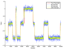
Figure 2: Markov chain parameter process and estimates obtained by adaptive filtering with $\varepsilon\ll O(\mu)$

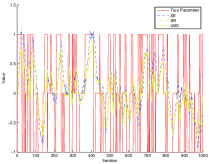
Figure 3: Markov chain parameter process and estimates obtained by adaptive filtering with $\varepsilon\gg\mu$

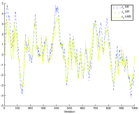
Figure 4: Scaled error $z_{n}$ with fast varying Markov chain ($\varepsilon\gg\mu$): Diffusion behavior

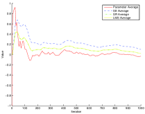
Figure 5: Average of parameter process and estimates over time with $\varepsilon\gg\mu$

To observe the tracking behavior of the SE algorithm, in comparison to the SR and LMS algorithms, we overlay the respective plots for each case. When $\varepsilon=O(\mu)$, the LMS and SR estimates tend to be approximately equal, while the SE estimates show more deviations from the other estimates. The SE algorithm responds to changes in the parameter more quickly, while the LMS and SR algorithms adhere to the parameter more closely while it is stationary. In the $\varepsilon\ll\mu$ case, we see this behavior repeated. While all three estimates track the parameter closely, the LMS and SR estimates deviate from the parameter less than the SE estimates between jumps of the parameter.

In the $\varepsilon\gg\mu$ case, none of the algorithms can track the parameter at each iterate very well. However, when we observe the scaled error against the stationary distribution of the Markov chain $z_{n}$, the expected diffusion behavior is displayed. Examining the cumulative average of the parameter and the estimates of the iterates, we note that the parameter average quickly converges to $\bar{\alpha}$. The LMS and SR estimate averages adhere closely to the parameter average, while the SE estimate average deviates slightly more.

References

- [1] A. Benveniste, M. Gooursat, and G. Ruget, Analysis of stochastic approximation schemes with discontinuous and dependent forcing terms with applications to data communication algorithms, IEEE Trans. Automatic Control, AC-25 (1980), 1042-1058.
- [2] A. Benveniste, M. Metivier, and P. Priouret, Adaptive Algorithms and Stochastic Approximations, Springer-Verlag, Berlin, 1990.
- [3] P. Billingsley, Convergence of Probability Measures, J. Wiley, New York, 1968.
- [4] H.-F. Chen, Stochastic Approximation and Its Applications, Kluwer Academic, Dordrecht, Netherlands, 2002.
- [5] H.-F. Chen and G. Yin, Asymptotic properties of sign algorithms for adaptive filtering, IEEE Trans. Automat. Control, 48 (2003), 1545–1556.
- [6] H.-F. Chen and G. Yin, On asymptotic properties of a constant-step-size sign-error algorithm for adaptive filtering, Science in China Series F: Information Sciences, 45 (2002), 321–334.
- [7] E. Eweda and O. Macchi, Quadratic mean and almost-sure convergence of unbounded stochastic approximation algorithms with correlated observations, Ann. Henri Poincaré, 19 (1983), 235-255.
- [8] E. Eweda, A tight upper bound of the average absolute error in a constant step size sign algorithm, IEEE Trans. Acoust. Speech Signal Proc., ASSP-37 (1989), 1774-1776.
- [9] E Eweda, Convergence of the sign algorithm for adaptive filtering with correlated data, IEEE Trans. Inform. Theory, IT-37 (1991), 1450-1457.
- [10] S.N. Ethier and T.G. Kurtz, Markov Processes, Characterization and Convergence, Wiley, New York, 1986
- [11] A. Gersho, Adaptive filtering with binary reinforcement, IEEE Trans. Inform. Theory, IT-30 (1984), 191-199.
- [12] L. Guo, Time-varying Stochastic Systems: Stability, Estimation and Control, Jilin Science Tech. Press, Changchun, 1993.
- [13] M.L. Honig, U. Madhow, and S. Verdu. Adaptive blind multiuser detection. IEEE Trans. Information Theory, 41 (1995) 944-960.
- [14] M.L. Honig and H.V. Poor, Adaptive interference suppression in wireless communication systems, in Wireless Communications: Signal Processing Perspectives, H.V. Poor and G.W. Wornell Eds., Prentice Hall, 1998.
- [15] H.J. Kushner, Approximation and Weak Convergence Methods for Random Processes, with Applications to Stochastic Systems Theory, MIT Press, Cambridge, MA, 1984.
- [16] H.J. Kushner and A. Shwartz, Weak convergence and asymptotic properties of adaptive filters with constant gains, IEEE Trans. Inform. Theory IT-30 (1984), 177–182.
- [17] H.J. Kushner and G. Yin, Stochastic Approximation and Recursive Algorithms and Applications, 2nd ed., Springer-Verlag, New York, NY, 2003.
- [18] C.P. Kwong, Dual signal algorithm for adaptive filtering, IEEE Trans. Comm. COM-34 (1986), 1272-1275.
- [19] L. Ljung, Analysis of stochastic gradient algorithms for linear regression problems, IEEE Trans. Inform. Theory, IT-30 (1984), 151-160.
- [20] O. Macchi and E. Eweda, Convergence analysis of self- adaptive equalizers, IEEE Trans. Information Theory, IT-30 (1984), 161-176.
- [21] M. Metivier and P. Priouret, Applications of a Kushner and Clark lemma to general classes of stochastic algorithms, IEEE Trans. Inform, Theory, IT-30 (1984), 140-151.
- [22] G.V. Moustakides, Exponential convergence of products of random matrices, application to adaptive algorithms, Internat. J. Adaptive Control Signal Process, 12 (1998), 579-597.
- [23] H.V. Poor and X. Wang. Code-aided interference suppression for DS/CDMA communications–Part I: Interference suppression capability, and Part II: Parallel blind adaptive implementations, IEEE Trans. Comm., 45 (1997), 1101-1111, and 1112–1122.
- [24] N.A.M. Verhoeckx, H.C. van den Elzen, F.A.M. Snijders, and P.J. van Gerwen, Digital echo cancellation for baseband data transmission, IEEE Trans. Acoust. Speech Signal Processing, 761-781.
- [25] L.Y. Wang, G. Yin, J.-F. Zhang, and Y.L. Zhao, System Identification with Quantized Observations: Theory and Applications, Birkhäuser, Boston, 2010.
- [26] B. Widrow and S.D. Stearns, Adaptive Signal Processing, Prentice-Hall, Englewood, Cliffs, NJ, 1985.
- [27] G. Yin, Adaptive filtering with averaging, in Adaptive Control, Filtering and Signal Processing, IMA Volumes in Mathematics and Its Applications, Vol. 74, 375–396, K. Aström, G. Goodwin and P.R. Kumar Eds., Springer-Verlag, New York, 1995.
- [28] G. Yin, A. Hashemi, and L.Y. Wang, Sign-regressor adaptive filtering algorithms for Markovian parameters, preprint, 2011.
- [29] G. Yin, C. Ion, and V. Krishnamurthy, How does a stochastic optimization/approximation algorithm adapt to a randomly evolving optimum/root with jump Markov sample paths, Math. Programming, Ser. B, 120 (2009), 67–99.
- [30] G. Yin, V. Krishnamurthy, and C. Ion, Iterate-averaging sign algorithms for adaptive filtering with applications to blind multiuser detection, IEEE Trans. Inform. Theory, 49 (2003), 657-671.
- [31] G. Yin, V. Krishnamurthy, and C. Ion, Regime switching stochastic approximation algorithms with application to adaptive discrete stochastic optimization, SIAM J. Optim., 14 (2004), 1187–1215.
- [32] G. Yin and V. Krishnamurthy, Least mean square algorithms with Markov regime switching limit, IEEE Trans. Automat. Control, 50 (2005), 577–593.
- [33] G. Yin and Q. Zhang, Discrete-time Markov Chains: Two-time-scale Methods and Applications, Springer, New York, NY, 2005.
- [34] G. Yin, Q. Zhang, and G. Badowski, Discrete-time singularly perturbed Markov chains: Aggregation, occupation measures, and switching diffusion limit, Adv. in Appl. Probab., 35(2), 449–476, 2003.
- [35] G. Yin and C. Zhu, Hybrid Switching Diffusions: Properties and Applications, Springer, New York, 2010.