The Dispersion Relations and Instability Thresholds of Oblique Plasma Modes in the Presence of an Ion Beam

Abstract

An ion beam can destabilize Alfvén/ion-cyclotron waves and magnetosonic/whistler waves if the beam speed is sufficiently large. Numerical solutions of the hot-plasma dispersion relation have previously shown that the minimum beam speed required to excite such instabilities is significantly smaller for oblique modes with $\mathbf{k}\times\mathbf{B}_{0}\neq 0$ than for parallel-propagating modes with $\mathbf{k}\times\mathbf{B}_{0}=0$, where $\mathbf{k}$ is the wavevector and $\mathbf{B}_{0}$ is the background magnetic field. In this paper, we explain this difference within the framework of quasilinear theory, focusing on low-$\beta$ plasmas. We begin by deriving, in the cold-plasma approximation, the dispersion relation and polarization properties of both oblique and parallel-propagating waves in the presence of an ion beam. We then show how the instability thresholds of the different wave branches can be deduced from the wave–particle resonance condition, the conservation of particle energy in the wave frame, the sign (positive or negative) of the wave energy, and the wave polarization. We also provide a graphical description of the different conditions under which Landau resonance and cyclotron resonance destabilize Alfvén/ion-cyclotron waves in the presence of an ion beam. We draw upon our results to discuss the types of instabilities that may limit the differential flow of alpha particles in the solar wind.

1. Introduction

The solar wind is a dilute plasma consisting of protons, electrons, and other ionic species. Among these other ions, the alpha particles play a special role due to their relatively high abundance. In the fast solar wind, for example, alpha particles comprise $\sim 15-20\%$ of the solar-wind mass density (Bame et al. 1977), which makes them dynamically and thermodynamically important.

In situ measurements have shown that the alpha particle velocity distribution is far from collisionally relaxed. For example, alpha particles generally have higher temperatures and outflow velocities than the protons. Also, like protons, alpha particles exhibit temperature anisotropy with $T_{\perp}\neq T_{\parallel}$, where $T_{\perp}$ ($T_{\parallel}$) measures the speed of thermal motions perpendicular (parallel) to the local magnetic field (Marsch et al. 1982; von Steiger et al. 1995; Neugebauer et al. 1996; Reisenfeld et al. 2001; Maruca et al. 2012). When measured in the proton frame, the beam speeds of alpha particles $U_{\rm i}$ seen in situ at heliocentric distances $r$ exceeding 0.3 AU is in most cases limited to a value of order the local Alfvén speed $v_{\mathrm{A}}$. At these heliocentric distances, the values of both $v_{\rm A}$ and $U_{\rm i}$ decrease with increasing $r$ while the proton speed is nearly constant. This means that an ongoing deceleration mechanism has to act on the alpha particles and regulate their drift speeds in interplanetary space.

Recent studies (Kasper et al. 2008; Bourouaine et al. 2011) have shown that $U_{\rm i}$ is anti-correlated with the collisional age $r\nu_{\rm col}/U$ of the solar wind, where $\nu_{\rm col}$ is the Coulomb collision frequency and $U$ is the proton outflow velocity. Under conditions of rare collisions in the measured solar wind interval, Bourouaine et al. (2011) found an upper threshold of about $1.2v_{\mathrm{A}}$ for $U_{\rm i}$ in Helios data at $r\sim 0.7\mbox{ AU}$. Several authors (e.g., Isenberg & Hollweg 1983; Gomberoff et al. 1996b; Kasper et al. 2008; Araneda et al. 2009) have argued that wave–particle interactions would lead to an upper limit of $U_{\mathrm{i}}\sim v_{\mathrm{A}}$. The study by Bourouaine et al. (2011) also found that solar-wind streams with $U_{\rm i}$ near this upper limit show excess magnetic fluctuation power at wavenumbers of up to the inverse local proton inertial length.

In situ observations suggest that the solar wind hosts a number of different plasma wave modes, including Alfvén waves (Belcher & Davis 1971; Tu & Marsch 1995), ion-cyclotron waves (Jian et al. 2010; He et al. 2012), whistler waves (Podesta & Gary 2011), and kinetic Alfvén waves (Bale et al. 2005; Salem et al. 2012). The properties of these waves depend on the properties of the plasma in which they propagate. One of these background properties is the composition of the plasma. Adding other ion species or relative drifts between the species modifies the waves significantly (Gomberoff & Elgueta 1991; Gnavi et al. 1996; Gomberoff et al. 1996a; Perrone et al. 2011; Marsch & Verscharen 2011; Verscharen & Marsch 2011). The above-mentioned alpha-particle beam is a typical example of such a drift. Apart from the modification of dispersion properties, the beam provides a source of free energy that can lead to the growth of electromagnetic instabilities, as shown in analytical and numerical studies (e.g., Montgomery et al. 1976; Gary 1993; Gary et al. 2000b; Li & Habbal 2000; Lu et al. 2006, 2009; Li & Lu 2010). These drift instabilities decelerate the drifting particle species to a stable value, thereby consuming the free energy source. These treatments discuss different types of instabilities and determine the threshold value of the relative drift at which the plasma becomes unstable. Some of the instabilities discussed include a circularly polarized parallel magnetosonic mode, an oblique magnetosonic mode, and two Alfvénic modes.The magnetosonic mode reaches its maximum growth rate at parallel propagation, at which the (previously studied) Alfvénic instabilities are suppressed (Montgomery et al. 1976). Gary et al. (2000b) have shown that the threshold drift speed for oblique Alfvénic instabilities is significantly smaller than for the parallel magnetosonic instability — $U_{\rm i}\gtrsim 0.8v_{\rm A}$ instead of $U_{\rm i}\gtrsim 1.7v_{\rm A}$, at least for situations in which the electron temperature is fairly large (four times the proton temperature in their study).

The intention of the present article is to give an analytical explanation for this behavior within the framework of quasilinear theory. Our primary objective is to elucidate the physics of these instabilities and not to refine or revise previous results on the values of these instability thresholds. We base our analysis on the cold-plasma dispersion relation, which we expect provides a reasonably accurate description of the real parts of the wave frequencies when $\beta\ll 1$, where $\beta=8\pi p/B^{2}$ is the ratio of the plasma pressure $p$ to the magnetic pressure. However, our use of the cold-plasma dispersion relation limits our analysis to the solar corona and the subset of solar-wind streams farther from the Sun that satisfy $\beta\ll 1$. Since most of the solar wind near 1 AU satisfy $\beta\sim 1$, our results do not describe the bulk of near-Earth solar wind. The remainder of this paper is organized as follows. In Section 2, we derive the cold-plasma dispersion relation for obliquely propagating plasma waves in the presence of an ion beam. We use the solutions of this dispersion relation to evaluate the wave polarization and wave energy. In Sections 3 and 4 we describe how the instability thresholds can be determined and understood in terms of (1) the resonance conditions for wave–particle interactions in quasilinear theory, (2) the conservation of resonant-particle kinetic energy in the reference frame moving with the wave along the background magnetic field, (3) the wave polarization, and (4) the sign (positive or negative) of the wave energy. In Section 5 we summarize our findings and discuss their application to alpha-particle beams in the solar wind.

We note that we do not address the details of the mechanism(s) that generate ion beams in the solar wind, which could be cyclotron-resonant wave–particle interactions (e.g., McKenzie & Marsch 1982; Hollweg & Isenberg 2002; Ofman et al. 2002), inhomogeneity effects with low-frequency waves (McKenzie et al. 1979; Isenberg & Hollweg 1982), stochastic heating by low-frequency waves (McChesney et al. 1987; Johnson & Cheng 2001; Chen et al. 2001; Chaston et al. 2004; Chandran 2010; Chandran et al. 2010), and/or some alternative process(es). Also, we concentrate on instabilities driven by resonant particles and not on the beam instabilities that are seen in solutions to the cold-plasma dispersion relation (Gomberoff et al. 1996a), in part because these “cold” instabilities have been found to be stabilized by the presence of other waves (Gomberoff 2003; Araneda & Gomberoff 2004).

2. Wave properties in a cold plasma

We consider a uniform, cold plasma consisting of three particle species: protons, electrons, and a population of beam ions. We assume that there is a uniform background magnetic field $\mathbf{B}_{0}=B_{0}\hat{\mathbf{e}}_{z}$, and that the electrons and beam ions flow with respect to the protons at average velocities $U_{\mathrm{e}}\hat{\mathbf{e}}_{z}$ and $U_{\mathrm{i}}\hat{\mathbf{e}}_{z}$, respectively, with $U_{\mathrm{i}}>0$ and $B_{0}>0$. We carry out all our calculations in the proton rest frame. We assume that on average the plasma is charge neutral, with

$$n_{\mathrm{p}}e+n_{\mathrm{i}}q_{\mathrm{i}}-n_{\mathrm{e}}e=0,$$ (1)

and carries (on average) zero current,

$$n_{\mathrm{i}}q_{\mathrm{i}}U_{\mathrm{i}}-n_{\mathrm{e}}eU_{\mathrm{e}}=0,$$ (2)

where $n_{\mathrm{p}}$, $n_{\mathrm{i}}$, and $n_{\mathrm{e}}$ are the proton, beam-ion, and electron number densities, and $e$ and $q_{\mathrm{i}}$ are the proton and beam-ion charges.

2.1. Dispersion Relation

We write the Fourier transform of the electric field in terms of its Cartesian components $E_{kx}$, $E_{ky}$, and $E_{kz}$. By linearizing Maxwell’s equations and the momentum equations for each particle species, we obtain an equation of the form

$$\frac{\mathbf{k}c}{\omega}\times\left(\frac{\mathbf{k}c}{\omega}\times\mathbf{E}_{k}\right)+\varepsilon\mathbf{E}_{k}\equiv\mathcal{D}\mathbf{E}_{k}=0,$$ (3)

where $\mathbf{k}=k_{\perp}\hat{\mathbf{e}}_{x}+k_{\parallel}\hat{\mathbf{e}}_{z}$ is the wavevector, $\omega$ is the frequency,

$$\varepsilon=\begin{pmatrix}S&-iD&J\\ iD&S&M\\ J&-M&P\end{pmatrix}$$ (4)

is the dielectric tensor, $S=(R+L)/2$, $D=(R-L)/2$, and the quantities

$$R=1-\sum\limits_{s}\left(\frac{\omega_{\mathrm{p}s}}{\omega}\right)^{2}\frac{\omega-k_{\parallel}U_{s}}{\omega-k_{\parallel}U_{s}+\Omega_{s}}$$ (5)

and

$$L=1-\sum\limits_{s}\left(\frac{\omega_{\mathrm{p}s}}{\omega}\right)^{2}\frac{\omega-k_{\parallel}U_{s}}{\omega-k_{\parallel}U_{s}-\Omega_{s}}$$ (6)

extend the notation of Stix (1992) to account for the relative drift between particle species. The plasma frequency of species $s$ is given by $\omega_{\mathrm{p}s}^{2}\equiv 4\pi n_{s}q_{s}^{2}/m_{s}$. The indices $\perp$ and $\parallel$ refer to the directions perpendicular and parallel to the background magnetic field. The gyrofrequency of the corresponding particle species is denoted $\Omega_{s}\equiv q_{s}B/(m_{s}c)$ and is negative for electrons. The terms

$$J=-\sum\limits_{s}\left(\frac{\omega_{\mathrm{p}s}}{\omega}\right)^{2}k_{\perp}U_{s}\frac{\omega-k_{\parallel}U_{s}}{\left(\omega-k_{\parallel}U_{s}\right)^{2}-\Omega_{s}^{2}}$$ (7)

and

$$M=i\sum\limits_{s}\left(\frac{\omega_{\mathrm{p}s}}{\omega}\right)^{2}k_{\perp}U_{s}\frac{\Omega_{s}}{\left(\omega-k_{\parallel}U_{s}\right)^{2}-\Omega_{s}^{2}}$$ (8)

represent new components of the dielectric tensor that are absent when the beam is absent, and

$$P=1-\sum\limits_{s}\left(\frac{\omega_{\mathrm{p}s}}{\omega}\right)^{2}\left[\frac{\omega^{2}}{\left(\omega-k_{\parallel}U_{s}\right)^{2}}+\frac{k_{\perp}^{2}U_{s}^{2}}{\left(\omega-k_{\parallel}U_{s}\right)^{2}-\Omega_{s}^{2}}\right].$$ (9)

The term “1” in the expressions for $R$, $L$, and $P$ stems from the displacement current and can be neglected in our study.

To obtain the dispersion relation, we set

$$\det\mathcal{D}=0.$$ (10)

We solve Equation (10) in two steps. First, we obtain approximate solutions to the dispersion relation in the limit that $m_{\mathrm{e}}\rightarrow 0$, where $m_{\rm e}$ is the electron mass. Second, we use this approximate solution as the starting point for a Newton’s-method solution to the full cold-plasma dispersion relation, taking into account the finite value of $m_{\rm e}/m_{\rm p}$.

In the limit $m_{\mathrm{e}}\rightarrow 0$, Equations (5) through (8) become

$$R \simeq\frac{\omega_{\mathrm{pp}}^{2}}{\Omega_{\mathrm{p}}\left(\Omega_{\mathrm{p}}+\omega\right)}+\frac{\omega_{\mathrm{pi}}^{2}\left(\omega-k_{\parallel}U_{\mathrm{i}}\right)^{2}}{\omega^{2}\Omega_{\mathrm{i}}\left(\Omega_{\mathrm{i}}+\omega-k_{\parallel}U_{\mathrm{i}}\right)},$$ (11)

$$L \simeq\frac{\omega_{\mathrm{pp}}^{2}}{\Omega_{\mathrm{p}}\left(\Omega_{\mathrm{p}}-\omega\right)}+\frac{\omega_{\mathrm{pi}}^{2}\left(\omega-k_{\parallel}U_{\mathrm{i}}\right)^{2}}{\omega^{2}\Omega_{\mathrm{i}}\left(\Omega_{\mathrm{i}}-\omega+k_{\parallel}U_{\mathrm{i}}\right)},$$ (12)

$$J \simeq-\left(\frac{\omega_{\mathrm{pi}}}{\omega}\right)^{2}k_{\perp}U_{\mathrm{i}}\frac{\omega-k_{\parallel}U_{\mathrm{i}}}{\left(\omega-k_{\parallel}U_{\mathrm{i}}\right)^{2}-\Omega_{\mathrm{i}}^{2}},$$ (13)

and

$$M\simeq i\left(\frac{\omega_{\mathrm{pi}}}{\omega}\right)^{2}\frac{k_{\perp}U_{\mathrm{i}}}{\Omega_{\mathrm{i}}}\frac{\left(\omega-k_{\parallel}U_{\mathrm{i}}\right)^{2}}{\left(\omega-k_{\parallel}U_{\mathrm{i}}\right)^{2}-\Omega_{\mathrm{i}}^{2}}.$$ (14)

As $m_{\mathrm{e}}\rightarrow 0$, $P\rightarrow\infty$, and only those terms in $\det\mathcal{D}$ that contain a factor of $P$ need to be retained when solving Equation (10). After factoring out this factor of $P$ from Equation (10), we obtain the ($m_{e}\rightarrow 0$) dispersion relation for Alfvén/ion-cyclotron and fast/whistler waves,

$$\left(\frac{kc}{\omega}\right)^{4}\cos^{2}\theta-\left(\frac{kc}{\omega}\right)^{2}\left(\frac{R+L}{2}\right)\left(1+\cos^{2}\theta\right)+RL=0,$$ (15)

where $\theta$ is the angle between $\mathbf{k}$ and $\mathbf{B}_{0}$. When $\theta=0$, Equation (15) becomes

$$\left[\left(\frac{kc}{\omega}\right)^{2}-L\right]\left[\left(\frac{kc}{\omega}\right)^{2}-R\right]=0.$$ (16)

Each of the equations $(kc/\omega)^{2}-L=0$ and $(kc/\omega)^{2}-R=0$ leads to a third-order polynomial equation for $\omega$. When the beam ions are alpha particles, the equation $(kc/\omega)^{2}-L=0$ is equivalent to Equation (2) of Gomberoff & Elgueta (1991). When $\theta\neq 0$, Equation (15) leads to a sixth-order polynomial equation for $\omega$, which we solve numerically using the Laguerre method (Press et al. 1992).

As mentioned above, we use our solution of Equation (15) as the starting point for a Newton’s-method solution of Equation (10) taking into account the finite electron mass. This second step to our solution of Equation (10) leads to only minor refinements to the wave frequency. However, it enables us to calculate polarization variables for each mode such as $E_{kz}/E_{kx}$, which are relevant to our discussion of Landau damping in the sections to follow.

For the remainder of this paper, we use the full solution of the cold-plasma dispersion relation with finite $m_{\rm e}$ rather than working in the zero-$m_{\rm e}$ limit. We also from here on restrict ourselves to the case in which the beam ions are alpha particles. We define

$$\eta\equiv\frac{n_{\mathrm{i}}}{n_{\mathrm{p}}}$$ (17)

and

$$v_{\mathrm{A}}\equiv\frac{B_{0}}{\sqrt{4\pi n_{\mathrm{p}}m_{\mathrm{p}}}}.$$ (18)

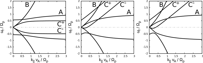
Figure 1.— Solutions to Equation (3) for an alpha-particle beam. The letters are explained in the text. For the left panel, $\eta=0.075$, $\theta=0^{\circ}$, and $U_{\mathrm{i}}=0$. For the middle panel, $\eta=0.05$, $\theta=1.5^{\circ}$, and $U_{\mathrm{i}}=1.1v_{\mathrm{A}}$. For the right panel, $\eta=0.05$, $\theta=45^{\circ}$, and $U_{\mathrm{i}}=1.1v_{\mathrm{A}}$.

In Figure 1, we plot $\mathrm{Re}\,\omega=\omega_{\mathrm{r}}$ for each of the six roots to Equation (15) for three different choices of $\eta$, $U_{\mathrm{i}}$, and $\theta$. We focus on four of these branches, which we label according to their asymptotic behaviors at large $k_{\parallel}$. Branch A is the proton-cyclotron branch, for which $\omega\rightarrow\Omega_{\rm p}$ as $k_{\parallel}\rightarrow\infty$. Branch B is the fast-magnetosonic/whistler branch, which behaves like a fast magnetosonic wave at $kv_{\rm A}/\Omega_{\rm p}<1$ and a whistler wave at $kv_{\rm A}/\Omega_{\rm p}>1$. Branch $\mbox{C}^{+}$ is the forward-propagating alpha-cyclotron branch, for which $\omega\rightarrow k_{\parallel}U_{\rm i}+\Omega_{\rm i}$ at large $k_{\parallel}$. In the frame of the alpha particles, the Doppler-shifted frequency of this wave $\omega-k_{\parallel}U_{\rm i}$ approaches $\Omega_{\rm i}$ as $k_{\parallel}\rightarrow\infty$. Branch $\mbox{C}^{-}$ is what we call the “counter-propagating” alpha-cyclotron branch. In the alpha-particle frame, this wave propagates in the $-z$ direction and has a Doppler-shifted frequency $\omega-k_{\parallel}U_{\rm i}$ that approaches $-\Omega_{\rm i}$ as $k_{\parallel}\rightarrow\infty$. We note that for each case shown, $\mathrm{Im}\,\omega=\gamma=0$ except at the intersections of different branches of the dispersion relation, where two branches have equal $\omega_{\mathrm{r}}$. In the right panel of Figure 1, this occurs, e.g., at $k_{\parallel}v_{\mathrm{A}}/\Omega_{\mathrm{p}}\approx 1.1$ and $\omega_{\mathrm{r}}\approx 0.7\Omega_{\mathrm{p}}$, where $\gamma\simeq\pm 0.02\Omega_{\mathrm{p}}$. Both solutions have the same absolute value of $\gamma$ but with opposite signs. Other modes can also merge in certain wavenumber ranges for different parameter choices. The magnetosonic mode B and the counter-propagating alpha-cyclotron mode C^- merge at higher drift speeds and show also a non-zero growth rate in the wavenumber range where they have equal $\omega_{\mathrm{r}}$. This unstable behavior of the cold-plasma dispersion relation is known as the ion–ion resonant instability (Gnavi et al. 1996; Gomberoff et al. 1996a).

2.2. Wave Polarization

The sense of circular or elliptical polarization of the waves can be defined in terms of the quantity

$$\mathcal{P}\equiv\frac{|E_{k,\mathrm{r}}|-|E_{k,\mathrm{l}}|}{|E_{k,\mathrm{r}}|+|E_{k,\mathrm{l}}|}=\frac{|\mathcal{A}-i|-|\mathcal{A}+i|}{|\mathcal{A}-i|+|\mathcal{A}+i|},$$ (19)

where $E_{k,\mathrm{r}}\equiv(E_{kx}-iE_{ky})/\sqrt{2}$ and $E_{k,\mathrm{l}}\equiv(E_{kx}+iE_{ky})/\sqrt{2}$. With the use of the $x$ and $y$ components of Equation (3), we can write

$$\mathcal{A}\equiv\frac{(S-n_{x}^{2}-n_{z}^{2})(J+n_{x}n_{z})+iDM}{(S-n_{z}^{2})M-iD(J+n_{x}n_{z})},$$ (20)

where $n_{x}=(kc/\omega)\sin\theta$ and $n_{z}=(kc/\omega)\cos\theta$. When $\theta=0$, we can use just the $x$ component of Equation (3) to obtain the simpler expression

$$\mathcal{A}\equiv\frac{iD}{S-n_{z}^{2}}.$$ (21)

Following the standard convention, we say that a wave is left (right) circularly polarized if the electric field vector in the $x$-$y$ plane rotates in the same sense as the cyclotron motion of a proton (electron). The connection between left/right circular polarization and the value of $\mathcal{P}$ depends upon the sign of the real part of the wave frequency $\omega_{\rm r}$. When $\omega_{\rm r}>0$, left-hand circular polarization corresponds to $\mathcal{P}=-1$, whereas right-hand circular polarization corresponds to $\mathcal{P}=1$. When $\omega_{\rm r}<0$, it is the reverse: left-hand circular polarization corresponds to $\mathcal{P}=1$ and right-hand circular polarization corresponds to $\mathcal{P}=-1$. In general, waves are not circularly polarized, but elliptically polarized with $\mathcal{P}\neq\pm 1$. Linear polarization corresponds to $\mathcal{P}=0$. The value of $\mathcal{P}$ is shown in Figure 2 for the case of oblique propagation.

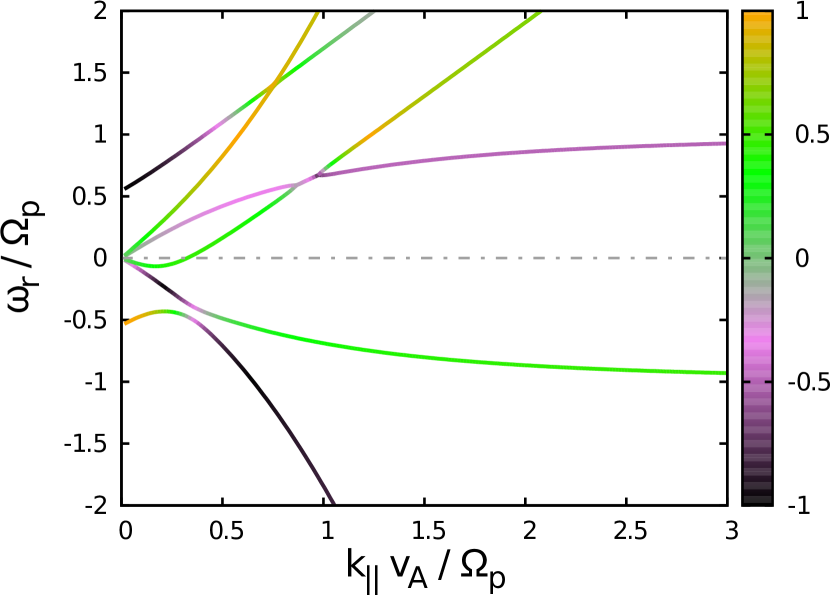
Figure 2.— The dispersion relation is shown for $\theta=45^{\circ}$, $\eta=0.05$, and $U_{\mathrm{i}}=1.2v_{\mathrm{A}}$. The color coding represents the polarization function $\mathcal{P}$. All modes in this diagram are elliptically polarized at oblique propagation.

It is instructive to consider the sense of polarization of the wave branches A, B, and $\mbox{C}^{\pm}$ in Figure 1 when $\theta=0$. It can be seen from Equations (16) and (21) that $\mathcal{P}=\pm 1$ when $\theta=0$, so that these wave branches are circularly polarized. More specifically, branch B is right-circularly polarized, and branches A and $\mbox{C}^{+}$ are left-circularly polarized. Branch $\mbox{C}^{-}$ is also left circularly polarized when $U_{\rm i}=0$, or, if $U_{\rm i}>0$, when $\omega_{\rm r}<0$. However, when $U_{\rm i}>0$ and $\omega_{\rm r}>0$, branch $\mbox{C}^{-}$ is right-circularly polarized. It is important to recall, however, that we have defined the sense of polarization in the rest frame of the protons. If we were to switch into the rest frame of the alpha particles, the Doppler-shifted wave frequency $\omega_{\rm r}-k_{\parallel}U_{\rm i}$ of branch $\mbox{C}^{-}$ would always be negative, and in this reference frame branch $\mbox{C}^{-}$ would appear to be left circularly polarized.

The longitudinal polarization is important for Landau-resonant interactions. We define the longitudinal polarization as

$$\mathcal{P}_{z}\equiv\left[\left|\frac{E_{kx}}{E_{kz}}\right|+\left|\frac{E_{ky}}{E_{kz}}\right|\right]^{-1}.$$ (22)

The right-hand side of Equation (22) can be evaluated with the use of the first two lines of Equation (3). It is found to be always much less than one for the treated modes. Its maximum value in the treated frequency and wavenumber range is of the order of $\mathcal{P}_{z}\lesssim 10^{-3}$. In parallel propagation, the determination of the parallel component of the electric field is not possible anymore via the first two components of Equation (3) since the dielectric tensor becomes block diagonal. The only parallel mode with $E_{kz}\neq 0$ is the $P=0$ mode, which has very high frequencies for the plasma conditions that we consider, and which is excluded here. Therefore, we can assume all parallel modes to have $E_{kz}=0$.

2.3. Wave Energy

The wave energy density per unit volume in $k$ space, denoted $W$, is given by

$$\left(2\pi\right)^{3}W=\frac{1}{8\pi}\left.\left[\mathbf{B}^{\ast}_{k}\cdot\mathbf{B}_{k}+\mathbf{E}^{\ast}_{k}\cdot\frac{\partial}{\partial\omega}(\omega\varepsilon_{\mathrm{h}})\mathbf{E}_{k}\right]\right|_{\omega=\omega_{\mathrm{r}}},$$ (23)

where $\mathbf{E}_{k}$ ($\mathbf{B}_{k}$) is the Fourier transform of the fluctuating electric (magnetic) field, and $\varepsilon_{\mathrm{h}}=(\varepsilon+\varepsilon^{\dagger})/2$ is the hermitian part of the dielectric tensor (Stix 1992, see also the discussion following Equation 27 of Chandran et al. 2010). The dagger symbol denotes the adjoint matrix. The factor of $\left(2\pi\right)^{3}$ on the left-hand side of Equation (23) does not appear in Equation (20) of Chapter 4 of Stix (1992). This difference arises because we define

$$\mathbf{E}_{k}=\int\mathbf{E}(\mathbf{x},t)e^{-i\mathbf{k}\cdot\mathbf{x}}\mathrm{d}^{3}x,$$ (24)

whereas Stix (1992) defines

$$\mathbf{E}_{k}=\left(2\pi\right)^{-3/2}\int\mathbf{E}(\mathbf{x},t)e^{-i\mathbf{k}\cdot\mathbf{x}}\mathrm{d}^{3}x.$$ (25)

This energy density describes both the energy density of the electromagnetic wave fields and the kinetic energy density of the particles under the assumption of a slow change of the wave amplitude with time.

It was found by Kadomtsev et al. (1965) that the term containing the derivative of the dielectric tensor in the expression for the wave energy can be negative and even lead to a situation in which waves have negative energy, meaning that $W<0$. In this case, the averaged kinetic energy of the particles plus the energy of the electromagnetic field is larger when the wave is absent than when it is present (Dawson 1961; Hollweg & Völk 1971). The behavior of negative-energy waves under the influence of dissipation is counter-intuitive. Dissipation, which removes energy from the fluctuations and converts it into heat, causes negative-energy waves to grow (Hall & Heckrotte 1966; Hollweg & Völk 1971). Similarly, if a negative-energy wave loses energy through a parametric instability, its own amplitude grows, increasing the rate of this instability. This is the so-called explosive instability (Oraevsky 1984). We find that the counter-propagating alpha-cyclotron wave C^- has negative energy for all $\omega_{\rm r}>0$. This situation is depicted in Figure 3. Negative-energy waves in the presence of an ion beam have been investigated previously by Gnavi et al. (1996).

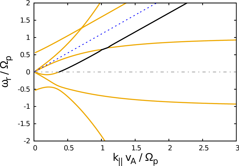
Figure 3.— Orange (black) color curves indicate positive (negative) values of the wave energy $W$ for the different solutions to the dispersion relation for $\theta=45^{\circ}$, $\eta=0.05$, and $U_{\mathrm{i}}=1.1v_{\mathrm{A}}$. The blue-dotted line indicates $\omega_{\mathrm{r}}=k_{\parallel}U_{\mathrm{i}}$.

In all cases that we have investigated so far, when the alpha-cyclotron branch merges with the proton-cyclotron or the magnetosonic mode, the resulting branches have negative energy throughout the finite interval of $k_{\parallel}$ in which the two branches have the same value of $\omega_{\rm r}$. This situation can be seen in Figure 3, where the forward propagating proton-cyclotron wave (branch A) and the alpha-cyclotron wave (branch C^-) that propagates backwards in the frame of the alpha particles merge.

3. Quasilinear Theory

Quasilinear theory provides an approximate, analytical description of wave–particle interactions in a collisionless plasma. One of the central assumptions of this theory is that the fluctuation amplitudes are sufficiently small that they can be described as a superposition of linear waves, and a particle’s orbit can be approximated as an unperturbed helix aligned with the background magnetic field. In addition, the theory assumes that the growth or damping rates of the waves are much smaller than the linear wave frequencies. The starting point of this theory is the Vlasov equation,

$$\frac{\partial f_{s}}{\partial t}+\mathbf{v}\cdot\frac{\partial f_{s}}{\partial\mathbf{x}}+\frac{q_{s}}{m_{s}}\left(\mathbf{E}+\frac{1}{c}\mathbf{v}\times\mathbf{B}\right)\cdot\frac{\partial f_{s}}{\partial\mathbf{v}}=0,$$ (26)

which describes the evolution of the distribution function $f_{s}(\mathbf{x},\mathbf{v},t)$ of particle species $s$ with mass $m_{s}$ and charge $q_{s}$ under the influence of the electric field $\mathbf{E}$ and magnetic field $\mathbf{B}$. In a constant homogeneous background magnetic field ($\mathbf{B}_{0}=B_{0}\hat{\mathbf{e}}_{z}$), a perturbation analysis leads to the following relation for the slow temporal evolution of the distribution function:

$$\frac{\partial f_{s}}{\partial t}=\lim_{V\to\infty}\sum\limits_{n=-\infty}^{+\infty}\frac{q_{s}^{2}}{8\pi^{2}m_{s}^{2}}\int\frac{1}{Vv_{\perp}}Gv_{\perp}\delta(\omega_{k\mathrm{r}}-k_{\parallel}v_{\parallel}-n\Omega_{s})\times\\ \times\left|\psi_{n,k}\right|^{2}Gf_{s}\mathrm{d}^{3}k,$$ (27)

where

$$G\equiv\left(1-\frac{k_{\parallel}v_{\parallel}}{\omega_{k\mathrm{r}}}\right)\frac{\partial}{\partial v_{\perp}}+\frac{k_{\parallel}v_{\perp}}{\omega_{k\mathrm{r}}}\frac{\partial}{\partial v_{\parallel}}$$ (28)

and

$$\psi_{n,k}\equiv\frac{1}{\sqrt{2}}\left[E_{k,\mathrm{r}}e^{i\phi}J_{n+1}(\sigma_{s})+E_{k,\mathrm{l}}e^{-i\phi}J_{n-1}(\sigma_{s})\right]\\ +\frac{v_{\parallel}}{v_{\perp}}E_{kz}J_{n}(\sigma_{s})$$ (29)

(Kennel & Engelmann 1966; Stix 1992). The azimuthal angle of the wavevector $\mathbf{k}$ is defined as $\phi$. The parallel and perpendicular components of the velocity in cylindrical coordinates are denoted $v_{\parallel}$ and $v_{\perp}$, respectively. The real part of the frequency that is a solution to the dispersion relation is denoted $\omega_{k\mathrm{r}}$. The amplitude function $\psi_{n,k}$ contains the Bessel function of $n$th order $J_{n}$ with the argument $\sigma_{s}\equiv k_{\perp}v_{\perp}/\Omega_{s}$. The quantity $V$ is a volume that is related to our Fourier transform convention. We treat the plasma as infinite and homogeneous. In order to make the Fourier transform of a function $h(\mathbf{x})$ converge, we first multiply this function by a window function $W$ that is $1$ inside a cubical region of volume $V$ centered on the origin and $0$ outside this volume. We then take the limit of $V\rightarrow\infty$.

Equation (27) shows that, in the framework of quasilinear theory, waves cause particles to diffuse in velocity space. Because of the delta function in Equation (27), particles of species $s$ with velocity $\mathbf{v}$ are affected by waves with wavevector $\mathbf{k}$ and frequency $\omega_{k\mathrm{r}}$ only if the waves and particles satisfy the resonance condition

$$\omega_{k\mathrm{r}}-k_{\parallel}v_{\parallel}=n\Omega_{s},$$ (30)

where $n$ is any integer. Equation (30) is called the Landau-resonance condition when $n=0$ and the cyclotron-resonance condition when $n\neq 0$. If there are only waves at a single $\mathbf{k}$ and $\omega_{k\mathrm{r}}$, then the diffusive flux of particles in velocity space is nonzero only within narrow bands of $v_{\parallel}$ that correspond to the solutions of Equation (30). Within those bands, the diffusive flux of particles is tangent to semicircles in the $v_{\parallel}$-$v_{\perp}$ plane defined by the equation

$$\left(v_{\parallel}-v_{\mathrm{ph}}\right)^{2}+v_{\perp}^{2}=\mathrm{constant},$$ (31)

where $v_{\mathrm{ph}}\equiv\omega_{k\mathrm{r}}/k_{\parallel}$ is the parallel phase velocity of the waves (Kennel & Engelmann 1966). When a spectrum of waves is present, velocity-space diffusion is not necessarily limited to narrow bands of $v_{\parallel}$ values, and particles can instead diffuse throughout an extended region in velocity space. For example, energetic protons undergoing cyclotron interactions with a broad spectrum of non-dispersive ($k_{\parallel}\ll\Omega_{\mathrm{p}}/v_{\mathrm{A}}$) Alfvén waves with dispersion relation $\omega_{k\mathrm{r}}=k_{\parallel}v_{\mathrm{A}}$ scatter along extended semi-circular arcs centered on $v_{\mathrm{A}}\hat{\mathbf{e}}_{z}$. In contrast, when wave–particle interactions are limited to the Landau resonance, particles can diffuse over an extended range in velocity space only if the spectrum of waves has a continuous range of $v_{\mathrm{ph}}$ values, because the Landau resonance only arises when $v_{\parallel}=v_{\mathrm{ph}}$. At each resonant value of $v_{\parallel}$, Landau-resonant interactions lead to diffusion only in $v_{\parallel}$, not in $v_{\perp}$, and so the extended diffusion paths for Landau-resonant interactions with a spectrum of waves are horizontal lines in the $v_{\parallel}$-$v_{\perp}$ plane. For our purposes, it is sufficient to consider the localized velocity-space diffusion that results from waves at a single $\mathbf{k}$ and $\omega_{k\mathrm{r}}$. In this case, Equation (31) determines the vector direction of the diffusive flux, up to a 180 degree ambiguity. This ambiguity can be resolved by noting that the net diffusive particle flux is directed from regions of higher particle concentration to regions of lower particle concentration in velocity space.

Bessel functions have the property $J_{n}(0)=\delta_{n,0}$, which shows that, for “slab” waves with $k_{\perp}=0$, resonances occur only when $n=-1$, 0, or 1 . We assume that

$$\sigma_{s}\ll 1,$$ (32)

set

$$J_{n}(\sigma_{s})\rightarrow\delta_{n,0},$$ (33)

and hence ignore resonances with $|n|>1$. Equation (32) is satisfied for Alfvén/ion-cyclotron waves and magnetosonic/whistler waves provided $\omega_{k\mathrm{r}}\lesssim\Omega_{\rm p}$, $\beta\ll 1$, and $\theta$ is not too close to $90^{\circ}$.

Throughout this paper, we work in the proton rest frame. This means that the parallel particle velocity $v_{\parallel}$ in the resonance condition (30) for the beam particles has two contributions, namely the beam velocity and the offset from the beam center. In some of the figures, we will plot “resonance lines”, which represent the condition $\omega_{\rm r}-k_{\parallel}v_{\parallel}=n\Omega_{\mathrm{i}}$. A solution of the resonance condition (Equation (30)) corresponds to an intersection of a resonance line and a plot of a dispersion relation $\omega_{\rm r}=\omega_{k\mathrm{r}}$. Since the distribution function of the alpha particles has a finite thermal width, we also plot a spread of the resonance lines taking particles into account that are slightly faster or slower than the bulk speed of the beam. The two resonance lines with the same $n$ then only represent the approximate upper and lower limits of parallel particle speeds that are available in the distribution function. Generally, there are always particles that can fulfill the resonance condition in the area between both plotted resonance lines with equal $n$. This is the only point in our considerations where thermal effects play a role, since we employ the cold-plasma dispersion relation. Some potential resonances are shown in Figure 4.

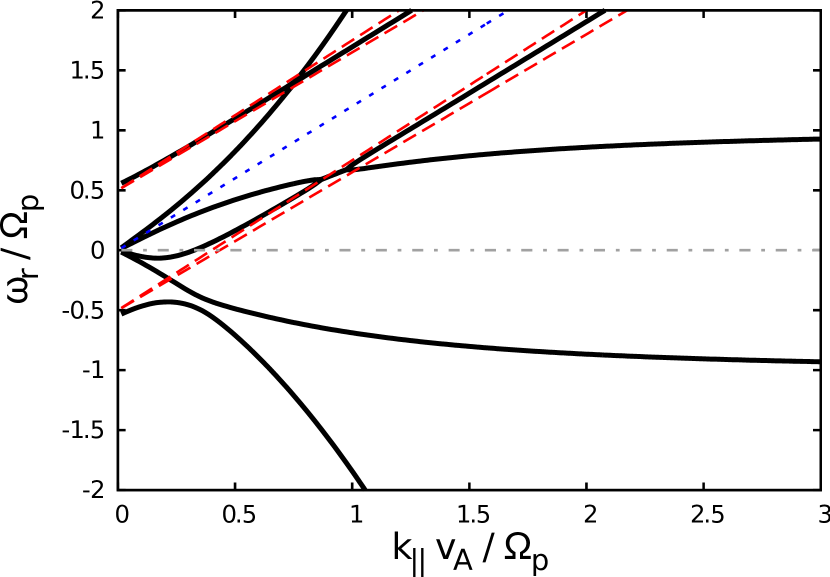
Figure 4.— Dispersion relation (black, solid) and cyclotron-resonance condition (red, dashed) for $\theta=45^{\circ}$, $U_{\mathrm{i}}=1.2v_{\mathrm{A}}$, and $\eta=0.05$. The blue dotted line represents $\omega_{\mathrm{r}}=k_{\parallel}U_{\mathrm{i}}$. The triple-dotted gray line corresponds to $\omega_{\mathrm{r}}=0$. The spread of the resonance lines corresponds to a parallel ion beta of $\beta_{\parallel\mathrm{i}}\simeq 10^{-4}$ for this choice of $\eta$.

Here we plot the six solutions in this wavenumber/frequency range to the dispersion relation, Equation (3). The red lines show the first two ($n=\pm 1$) cyclotron resonances for alpha particles with parallel velocities $v_{\parallel}=U_{\mathrm{i}}\pm 0.05v_{\mathrm{A}}$. We take $\Delta v_{\parallel}=\left|v_{\parallel}-U_{\mathrm{i}}\right|$ to correspond to twice the parallel thermal speed $v_{\mathrm{thi}}\equiv\sqrt{2k_{\mathrm{B}}T_{\parallel\mathrm{i}}/m_{\mathrm{i}}}$ of the alpha particles on the assumption that there are too few alpha particles with $\Delta v_{\parallel}>2v_{\mathrm{thi}}$ to drive a significant instability. This situation corresponds to a plasma with

$$\beta_{\parallel\mathrm{i}}\equiv\frac{8\pi n_{\rm i}k_{\rm B}T_{\parallel\rm i}}{B_{0}^{2}}=\left(\frac{n_{\rm i}m_{\rm i}}{n_{\rm p}m_{\rm p}}\right)\left(\frac{v_{\mathrm{thi}}}{v_{\rm A}}\right)^{2}\simeq 10^{-4}$$ (34)

where $T_{\parallel\rm i}$ is the parallel ion (alpha-particle) temperature. The Landau resonance, which is only acting if $E_{kz}\neq 0$ or $k_{\perp}\neq 0$, is located on resonance lines with a small spread around the line $\omega_{\mathrm{r}}=k_{\parallel}U_{\mathrm{i}}$, which corresponds to the vicinity of the blue-dotted line in Figure 4.

4. Instability Thresholds

In this paper, we focus on instabilities driven by the velocity-space diffusion of alpha particles that interact resonantly with the unstable wave. Some possible velocity-space diffusion paths for a beam of alpha particles are shown in Figure 5 for the cyclotron-resonant case and in Figure 6 for the Landau-resonant case based on the assumption that the particle distribution functions are isotropic about the mean velocity of the particle species.

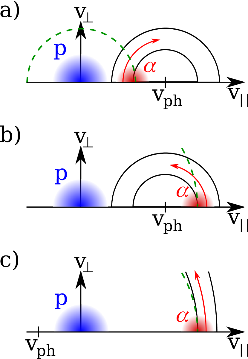
Figure 5.— Direction of the diffusive particle flux for cyclotron-resonant alpha particles. The regions occupied by thermal protons (alpha particles) are shown as blue (red) filled circles. The arrows and circles show the diffusion paths around the position of the parallel phase speed $v_{\mathrm{ph}}$ for a cyclotron resonance. The green dashed lines are iso-contours of the kinetic energy in the proton frame. a) $U_{\mathrm{i}}<v_{\mathrm{ph}}$, b) $U_{\mathrm{i}}>v_{\mathrm{ph}}$, c) $v_{\mathrm{ph}}<0$.

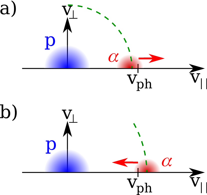
Figure 6.— Direction of the diffusive particle flux for Landau-resonant alpha particles. The regions occupied by thermal protons (alpha particles) are shown as blue (red) filled circles. The arrows show the diffusion paths at the position of the parallel phase speed $v_{\mathrm{ph}}$ for a Landau resonance. The green dashed lines are iso-contours of the kinetic energy in the proton frame. a) $U_{\mathrm{i}}<v_{\mathrm{ph}}$, b) $U_{\mathrm{i}}>v_{\mathrm{ph}}$.

The resonant alpha particles diffuse down the density gradient in velocity space, from larger particle concentrations towards smaller particle concentrations along the diffusion paths. We concentrate on the normal case with positive wave energy first. In this case, if the particles gain energy during the resonant quasilinear diffusion, the energy is taken from the wave, and the wave is damped. On the other hand, if the particles diffuse towards smaller particle energies, then the energy lost by the particles is given to the wave, leading to wave amplification. To see whether particles gain or lose energy, the quasilinear-diffusion paths can be compared with curves of constant particle energy, which are circles centered on the origin in the $v_{\parallel}$-$v_{\perp}$ plane. The key point demonstrated by Figure 5 is that cyclotron-resonant wave–particle interactions cause alpha particles to lose energy if and only if $0<v_{\mathrm{ph}}<U_{\mathrm{i}}$. Therefore, if $W>0$, the wavevectors and frequencies of unstable waves must lie above the line $\omega_{\rm r}=0$ and below the line $\omega_{\mathrm{r}}=k_{\parallel}U_{\mathrm{i}}$ in the $k_{\parallel}$-$\omega_{\mathrm{r}}$ plane. Figure 6 demonstrates that the same requirement is also valid for Landau-resonant particles. A mathematical proof of the instability condition $0<v_{\mathrm{ph}}<U_{\mathrm{i}}$ is given in the Appendix.

For simplicity, we take the protons to be Maxwellian for the purposes of inferring the effects of wave–particle interactions on the waves. We thus neglect proton temperature anisotropy and proton beams. As a consequence, if protons diffuse in velocity space from regions of large particle concentration towards regions of small particle concentration, then they must gain energy. Because the protons are the majority ion species, we expect that proton damping will dominate over the alpha-particle instability drive if thermal protons can resonate with a wave.

The foregoing discussion and the condition $\sigma_{s}\ll 1$ imply that a solution of the dispersion relation with $\mathbf{k}=\mathbf{k}_{1}$, $\omega_{k\mathrm{r}}=\omega_{1}$, and $W>0$ is driven unstable by resonant interactions with an alpha-particle beam that is isotropic about the beam velocity $U_{\mathrm{i}}$ in $v$-space if and only if the following conditions are satisfied:

1. The coordinates ($k_{1\parallel}$, $\omega_{1}$) lie between two resonance lines with equal $n$ with $n=+1$, $n=0$, or $n=-1$. If ($k_{1\parallel}$, $\omega_{1}$) lies between two resonance lines with $n=-1$, then we say that the instability is driven by an $n=-1$ resonance, and likewise for $n=0$ and $n=+1$.

2. For an instability driven by an $n=+1$ resonance, $E_{k,\rm l}$ must be nonzero (i.e., $\mathcal{P}\neq+1$). For an instability driven by an $n=-1$ resonance, $E_{k,\rm r}$ must be nonzero (i.e., $\mathcal{P}\neq-1$). For an instability driven by an $n=0$ resonance, $E_{kz}$ or $k_{\perp}$ must be nonzero.

3. The parallel phase velocity of the waves is between zero and the beam speed: $0<\omega_{1}/k_{1\parallel}<U_{\mathrm{i}}$.

4. The wave at $\mathbf{k}_{1}$ and $\omega_{1}$ does not satisfy the resonance condition Equation (30) with thermal protons.

Condition 2 above on the wave polarization follows from substituting Equation (33) into Equation (29). Importantly, a mode with $W<0$ that satisfies the above criteria is damped, because an increase in the energy of a negative-energy wave corresponds to a decrease in the wave’s amplitude. In the next two subsections, we use the above criteria to determine which branches of the dispersion relation are unstable and at which wavenumbers as a function of the beam velocity, the angle of propagation, and the parallel thermal widths of the alpha and proton distributions.

4.1. Parallel Case ($k_{\perp}=0$)

The Landau resonance $n=0$ can be excluded for fast modes and cyclotron modes when $k_{\perp}=0$ because $E_{kz}=0$ (so that Landau damping is absent) and because transit-time damping (the other type of $n=0$ resonance) requires $k_{\perp}\neq 0$ (Stix 1992). The counter-propagating alpha-cyclotron mode (branch $\mbox{C}^{-}$ in Figure 1) appears to be a candidate for an instability driven by the $n=-1$ resonance with the alpha particle beam, because it satisfies the four criteria for instability listed above when $\omega_{k\rm r}>0$, even for modest beam speeds such as $U_{\rm i}=0.5v_{\rm A}$, which can be seen with the aid of Figure 7. However, this mode has negative energy when $\omega_{k\rm r}>0$, as illustrated in Figure 3, and is therefore stable.

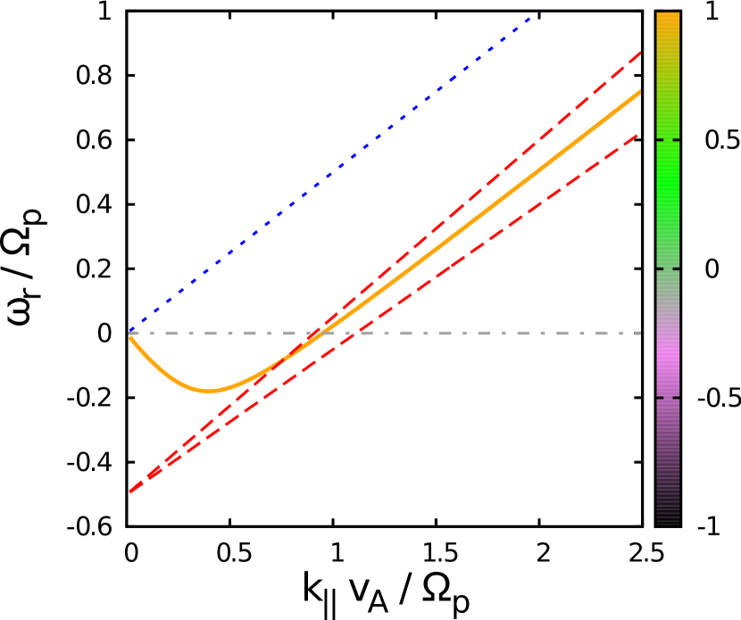
Figure 7.— Dispersion and polarization for $U_{\mathrm{i}}=0.5v_{\mathrm{A}}$, $\eta=0.05$, and $\theta=0^{\circ}$. The color coding shows the polarization $\mathcal{P}$. Only branch C^- is shown. The two red lines are the resonance lines for $n=-1$. The dotted blue line shows the maximum frequency $\omega_{\mathrm{r}}=k_{\parallel}U_{\mathrm{i}}$, and the triple-dotted gray line is the minimum frequency $\omega_{\mathrm{r}}=0$.

If $\beta_{\parallel\rm i}$ is sufficiently large, then alpha particles can satisfy the $n=+1$ resonance condition with the Alfvén/proton-cyclotron wave (branch A in Figure 1) and potentially drive this mode unstable. To the best of our knowledge, such a parallel Alfvén instability has not been described previously in the literature, although it might play an important role in the solar wind. We note, however, that our approximations break down when $\beta\gtrsim 1$, because we have approximated the wave frequencies using the cold-plasma dispersion relation. In order to investigate parallel Alfvén/cyclotron instabilities at large $\beta_{\parallel\rm i}$ rigorously, a more sophisticated approach based on the full hot-plasma dispersion relation would be needed.

Although the counter-propagating alpha-cyclotron branch C^- is stable when $k_{\perp}=0$, the fast-magnetosonic/whistler mode becomes unstable at sufficiently large $U_{\rm i}$ due to the $n=-1$ resonance with the alpha particles. When $\Delta v_{\parallel}=2v_{\mathrm{thi}}=0.35v_{\mathrm{A}}$, the minimum value of $U_{\rm i}$ for this instability is $\simeq 1.7v_{\rm A}$. With the given alpha-particle density, this situation corresponds to a plasma with $\beta_{\parallel\mathrm{i}}\simeq 0.006$. These parameters are illustrated on the left-hand side in Figure 8, and it can be seen from this figure that this instability satisfies all four criteria in the above list. This instability corresponds to the parallel magnetosonic instability discussed by Daughton & Gary (1998) and Gary et al. (2000a), and sets in at a typical wavenumber of order the inverse proton inertial length $\Omega_{\rm p}/v_{\rm A}$. The left-hand side in Figure 8 furthermore shows that at this drift speed but at a lower thermal speed the resonance lines do not intersect with the plot of the dispersion relation of the magnetosonic branch. This lower thermal speed represents a situation with a lower $\beta_{\parallel\mathrm{i}}$ provided the fractional number density $\eta$ is constant. As $\Delta v_{\parallel}$ is decreased below $0.3v_{\mathrm{A}}$, it becomes increasingly difficult to excite this instability for two reasons. First, the value of $U_{\rm i}$ needs to be increased simply in order to get the $n=-1$ resonance line to intersect the dispersion-relation curve for the forward-propagating fast-magnetosonic/whistler mode. Second, at these larger values of $U_{\rm i}$, the fast-magnetosonic/whistler branch B merges with the counter-propagating alpha-cyclotron branch C^- throughout a finite interval of $k_{\parallel}$ (i.e., they have the same value of $\omega_{k\mathrm{r}}$). Within this interval, $W<0$ for both modes, and any intersection of an $n=-1$ resonance line with either mode’s dispersion relation is unable to generate an instability according to the above four criteria.

As $v_{\mathrm{thi}}$ is increased, our quasilinear/cold-plasma analysis suggests that the threshold for this instability moves to smaller $U_{\rm i}$, because larger alpha-particle thermal speeds enable the alpha-particle $n=-1$ resonance lines to intersect with the fast-magnetosonic/whistler dispersion relation at smaller values of $U_{\rm i}$. This situation is shown on the right-hand side of Figure 8. With $\eta=0.05$, this situation corresponds to $\beta_{\parallel\mathrm{i}}\simeq 0.02$. The growth rate dependence of the magnetosonic instability on the thermal speed of the beam has been calculated by Daughton & Gary (1998) for a proton-beam plasma. In qualitative agreement with our arguments, they have shown that the growth rate increases for higher temperatures of the beam.

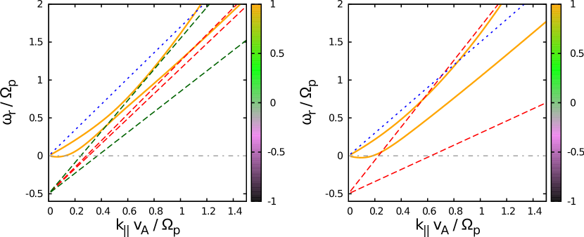
Figure 8.— Dispersion relation and polarization of the branches B and C^- for $\eta=0.05$ and $\theta=0$. The color coding shows the polarization $\mathcal{P}$. The resonance lines for $n=-1$ are shown for different thermal speeds. The dotted blue line shows the maximum frequency $\omega_{\mathrm{r}}=k_{\parallel}U_{\mathrm{i}}$, and the triple-dotted gray line is the minimum frequency $\omega_{\mathrm{r}}=0$. Left: $U_{\mathrm{i}}=1.7v_{\mathrm{A}}$. The thermal spread corresponds to $\Delta v_{\parallel}=2v_{\mathrm{thi}}=0.05v_{\mathrm{A}}$ for the red resonance lines and to $\Delta v_{\parallel}=2v_{\mathrm{thi}}=0.35v_{\mathrm{A}}$ for the green resonance lines. Right: $U_{\mathrm{i}}=1.5v_{\mathrm{A}}$ and $\Delta v_{\parallel}=2v_{\mathrm{thi}}=0.7v_{\mathrm{A}}$.

4.2. Oblique Case ($k_{\perp}\neq 0$)

A moderate obliquity does not significantly change the structure of the dispersion branches A, B, and $\mbox{C}^{\pm}$ in Figure 1. It does, however, change the polarization. When $k_{\perp}\neq 0$, the waves are in general elliptically polarized and can interact with particles via both the $n=+1$ and $n=-1$ cyclotron resonances. Furthermore, Landau-resonant interactions (with $n=0$) are now possible, because $E_{kz}$ becomes nonzero for oblique waves, and the nonzero value of $k_{\perp}$ allows for transit-time damping.

The magnetosonic instability that was present in the parallel case (Section 4.1) is also present in the oblique case. However, whereas the parallel magnetosonic mode resonantly interacts with the alpha particles only through the $n=-1$ cyclotron resonance, the oblique magnetosonic mode can interact with alpha particles through either the $n=-1$ cyclotron resonance or the $n=0$ Landau resonance. For low drift speeds $U_{\mathrm{i}}\gtrsim v_{\mathrm{A}}$, the resonance condition with $n=0$ is fulfilled at lower values for $k_{\parallel}$ than the resonance condition with $n=-1$. The two resonance conditions are, therefore, expected to act on the magnetosonic mode in different wavenumber regimes. In the small-wavenumber limit, the fast-wave dispersion relation is $\omega_{k\rm r}=kv_{\rm A}$, and the instability condition $U_{\rm i}>\omega_{k\rm r}/k_{\parallel}$ becomes $U_{\rm i}>v_{\rm A}/\cos\theta$. This argument suggests that the threshold value of the drift speed for the oblique magnetosonic instability is higher at larger $\theta$.

The intersection of the $n=-1$ resonance line with the dispersion relation for proton-cyclotron waves can fulfill constraint 2 for oblique waves due to their elliptical polarization. To fulfill constraint 4, the drift speed should be larger than $U_{\mathrm{i}}\approx 1.2v_{\mathrm{A}}$. Then the intersection of the resonance line and the dispersion relation for oblique Alfvén/proton-cyclotron waves occurs at low enough frequencies and wavenumbers ($k_{\parallel}v_{\mathrm{A}}/\Omega_{\mathrm{p}}\lesssim 1$) that proton damping can be ignored. This is the situation in Figure 9, which also shows the wave polarization.

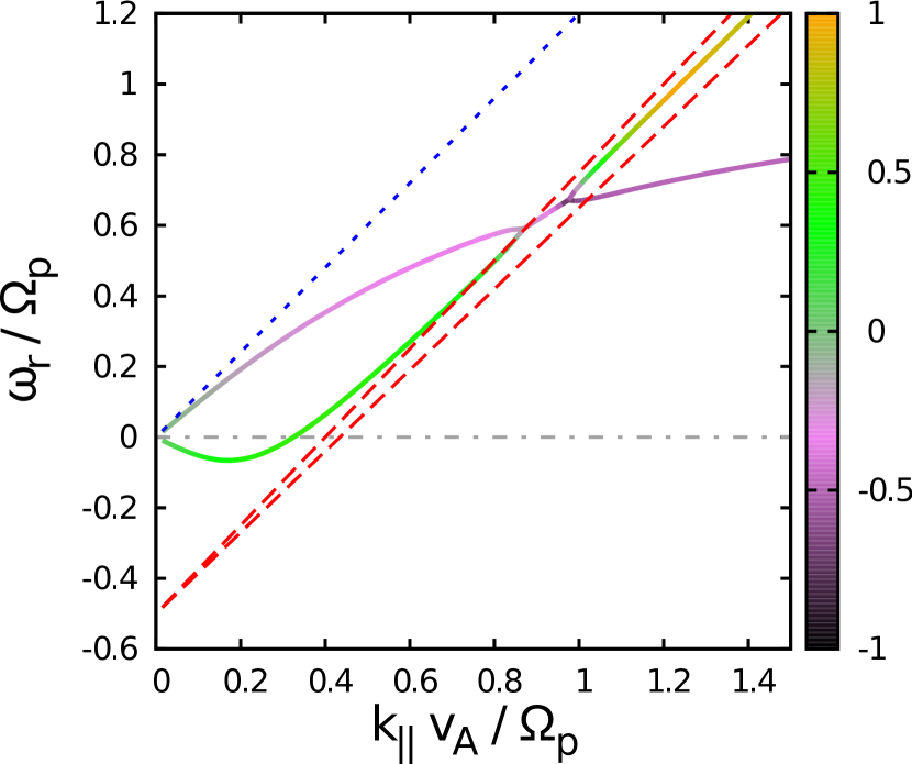
Figure 9.— Dispersion relation and polarization for the wave branches A and C^-. The same parameter set as in Figure 4 is used. The color coding shows the value of the polarization function $\mathcal{P}$.

We identify this instability with the Alfvén I instability discussed by Gary et al. (2000b). It begins at $U_{\mathrm{i}}\gtrsim 1.2v_{\mathrm{A}}$. There is a finite interval of $k_{\parallel}$ in which the proton cyclotron wave and the counter-propagating alpha-cyclotron wave (branches A and $\mbox{C}^{-}$ in Figure 1) merge — i.e., in which the two waves have the same value of $\omega_{k\rm r}$. Within this wavenumber interval, both waves have negative energy, and neither is driven unstable by resonant particles.

Another instability that becomes possible at oblique propagation is the so-called Alfvén II instability. We identify this instability with the forward-propagating proton-cyclotron mode, when this mode is driven unstable by Landau-resonant interactions with the alpha-particle beam. According to the third of the four criteria laid out at the beginning of Section 4, this instability requires that $U_{\rm i}>\omega_{k\rm r}/k_{\parallel}$. The parallel phase velocity $\omega_{k\rm r}/k_{\parallel}$ of the proton-cyclotron wave is $v_{\rm A}$ for $k_{\parallel}\ll\Omega_{\rm p}/v_{\rm A}$ and decreases towards zero at $k_{\parallel}\rightarrow\infty$. Thus, the condition $U_{\rm i}>\omega_{k\rm r}/k_{\parallel}$ is always satisfied for positive $U_{\rm i}$ provided that $k_{\parallel}$ is sufficiently large. However, if $k_{\parallel}$ is too large, criterion 4 in the above list is not satisfied, because $\omega_{k\rm r}\sim\Omega_{\rm p}$ and the wave is damped by cyclotron resonant interactions with protons. In order to avoid proton cyclotron damping, $k_{\parallel}$ must be $\lesssim\Omega_{\rm p}/v_{\rm A}$ (the precise upper limit depends upon the value of $\beta_{\parallel\rm p}$ for the protons). In order to have $U_{\rm i}>\omega_{k\rm r}/k_{\parallel}$ at $k_{\parallel}<\Omega_{\rm p}/v_{\rm A}$, $U_{\rm i}$ must exceed $\simeq 0.8v_{\rm A}$, which is the approximate threshold-value of $U_{\rm i}$ for this instability. This case is shown in Figure 10.

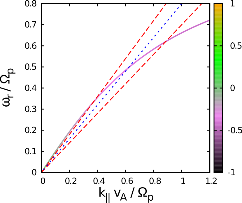
Figure 10.— Dispersion relation and polarization for the wave branch A with $\theta=45^{\circ}$, $\eta=0.05$, and $U_{\mathrm{i}}=0.8v_{\mathrm{A}}$. The color coding shows the value of the polarization function $\mathcal{P}$. The resonance lines represent the Landau resonance with $n=0$ and $\Delta v_{\parallel}=2v_{\mathrm{thi}}=0.1v_{\mathrm{A}}$. Only resonance lines below the line $\omega_{\mathrm{r}}=k_{\parallel}U_{\mathrm{i}}$ can drive the Alfvén II instability according to criterion 3.

Criterion three in the above list of four criteria, combined with the Landau resonance condition $\omega_{k\rm r}/k_{\parallel}=v_{\parallel}$, imply that only alpha particles with $v_{\parallel}<U_{\rm i}$ can drive the Alfvén II instability. As $U_{\rm i}$ is increased beyond $v_{\rm A}$, fewer and fewer alpha particles can undergo a Landau resonance with the proton-cyclotron wave, and thus there is an upper limit on $U_{\rm i}$ for the Alfvén II instability. As $\beta_{\parallel\rm i}$ increases for the alpha particles, this upper limit increases.

There is evidence in previous treatments of beam instabilities that another kinetic effect may weaken or suppress the oblique instabilities in certain parameter regimes. It was found by Montgomery et al. (1976) in a proton-beam plasma that the oblique Alfvénic instability (which corresponds to Alfvén II according to Daughton & Gary 1998) shows a higher growth rate at greater values of $T_{\mathrm{e}}/T_{\mathrm{p}}$, whereas the cyclotron-resonant magnetosonic instability does not. Montgomery et al. (1976) interpreted this result as a consequence of Landau-damping of these modes by electrons. At higher electron temperatures, the gradients of the electron distribution function in velocity space become smaller since the width of the distribution function increases. The influence of electron Landau damping is determined by these gradients and, therefore, mitigated at higher electron temperatures. In our model, the Landau-resonance condition for electrons would correspond to resonance lines that are very widely spread due to their large thermal speed. Therefore, almost all waves with $\mathcal{P}_{z}\neq 0$ in our frequency range can undergo electron Landau damping. The Alfvén I instability may not be as strongly influenced by this effect as the Landau-resonant instabilities since the Alfvén I instability generally shows higher growth rates in the numerical solutions of the hot-plasma dispersion relation under typical parameters (e.g., Gary et al. 2000b). This effect may also be the reason why Montgomery et al. (1976) find that the oblique magnetosonic instability has a significant growth rate over only a very small range of the plasma parameters, and why Gary et al. (2000b) do not discuss this mode for a proton-alpha plasma. The details of this effect, however, require a deeper study and are beyond the scope of this work.

5. Discussion and Conclusions

In this paper, we use quasilinear theory to explain the thresholds for Alfvén/ion-cyclotron and magnetosonic/whistler instabilities driven by resonant interactions with an alpha-particle beam in low-$\beta$ plasmas. Our arguments rely upon three properties of the wave modes in question: the real part of the wave frequency $\omega_{k\rm r}$, the polarization of the wave electric field, and the sign of the wave energy density $W$. (See Section 2.3 for a discussion of negative-energy waves.) To obtain approximate values for these quantities as functions of the wavevector $\mathbf{k}$, we have used the cold-plasma approximation, taking into account the finite electron mass.

The general considerations that determine whether a wave is driven unstable by resonant interactions with a beam of alpha particles are the following. First, in order for a wave to be unstable at some value of $k_{\parallel}$, it can not undergo cyclotron resonant interactions with the thermal protons at that $k_{\parallel}$, since such interactions would strongly damp the wave. Second, the wave and alpha particles must satisfy the wave–particle resonance condition, Equation (30). Third, the resonant wave–particle interactions must cause the alpha particles to lose energy, so that the wave can gain energy and grow. (This statement assumes that $W>0$ — more details on the stability and instability of negative-energy waves are given in Section 4). As we show in Section 4 and in the Appendix, resonant wave–particle interactions cause alpha particles with a distribution function that is isotropic about their mean velocity to lose energy when $0<\omega_{k\mathrm{r}}/k_{\parallel}<U_{\rm i}$, where $U_{\rm i}$ is the speed of the alpha particle beam, and all quantities (e.g., $\omega_{k\mathrm{r}}$, $U_{\rm i}$) are measured in the proton rest frame. Fourth, the wave polarization must satisfy the following conditions. In order for a wave to be driven unstable by an $n=+1$ ($n=-1$) cyclotron resonance, $E_{k,\rm l}$ ($E_{k,\rm r}$) must be nonzero. When $k_{\perp}=0$, a wave can be driven unstable by the $n=0$ Landau resonance only when $E_{kz}\neq 0$.

When we apply these considerations to parallel waves with $k_{\perp}=0$, we find that alpha particles are unable to drive resonant instabilities when $\Delta v_{\parallel}=2v_{\mathrm{thi}}$ is much smaller than $0.35$. When $\Delta v_{\parallel}\simeq 0.35$, our criteria suggest that the magnetosonic/whistler wave becomes unstable via the $n=-1$ resonance when $U_{\rm i}$ exceeds $\sim 1.7v_{\rm A}$, consistent with previous numerical results (Li & Habbal 2000; Gary et al. 2000a). Our arguments suggest that this minimum threshold on $U_{\rm i}$ decreases slightly as the parallel thermal speed of the ions increases further. Our arguments also suggest that as $v_{\mathrm{thi}}$ (and therefore $\beta_{\parallel\mathrm{i}}$) increases, the alpha particles eventually drive the proton-cyclotron wave (branch A in Figure 1) unstable in the $n=+1$ resonance. We note, however, that our conclusions about the high-$\beta_{\parallel\rm i}$ case must be treated with caution, because of our use of the cold-plasma dispersion relation.

When we apply the above instability criteria to oblique waves with $k_{\perp}\neq 0$, we find that the magnetosonic mode can still be unstable, but that it can now be rooted in either the cyclotron resonance ($n=-1$) or the Landau resonance ($n=0$). The minimum threshold to excite the oblique magnetosonic instability via the Landau resonance is somewhat smaller than for the parallel magnetosonic instability, and also less dependent on $v_{\mathrm{thi}}$. The wavenumbers at which the mode is unstable when driven by the $n=0$ resonance are smaller than the unstable wavenumbers for oblique magnetosonic instabilities driven by the $n=-1$ resonance. At these smaller wavenumbers, the dispersion relation of the magnetosonic mode for the $n=0$ resonant instability can be approximated by $\omega_{k\mathrm{r}}\approx k_{\parallel}v_{\mathrm{A}}/\cos\theta$ which leads to an instability threshold of $U_{\mathrm{i}}\gtrsim v_{\mathrm{A}}/\cos\theta$ according to the instability criterion 3 introduced in Section 4. At oblique propagation, there are also two types of Alfvén/cyclotron instabilities that are not present at parallel propagation. The first of these, the “Alfvén I” instability, is driven by the $n=-1$ cyclotron resonance. Our analysis suggests that this instability requires $U_{\rm i}\gtrsim 1.2v_{\rm A}$, which is consistent with the numerical results of Gary et al. (2000b) for a plasma with $T_{\mathrm{e}}/T_{\mathrm{p}}=4$. Our physical interpretation of this instability threshold is that it is the minimum value of $U_{\rm i}$ for which alpha particles can resonate with the proton-cyclotron wave (branch A in Figure 1) through the $n=-1$ resonance at a wavenumber $k_{\parallel}$ that is sufficiently small to avoid strong cyclotron damping by the protons. The second oblique instability, the so-called Alfvén II instability (Daughton & Gary 1998; Gary et al. 2000b), is driven by the $n=0$ Landau resonance. Our arguments suggest that this instability requires that $U_{\rm i}\gtrsim 0.8v_{\rm A}$, consistent with the numerical results of Gary et al. (2000b) for the case in which $T_{\rm e}/T_{\rm p}=4$. This lower threshold on $U_{\rm i}$ is the minimum beam speed for which the proton-cyclotron wave (branch A in Figure 1) can undergo a Landau ($n=0$) resonance with the alpha particles at a $k_{\parallel}$ that is sufficiently small to avoid strong proton cyclotron damping. We note, however, as discussed in Section 4.2, that the Alfvénic instabilities and the oblique magnetosonic instability may weaken as $T_{\rm e}/T_{\rm p}$ decreases because of the more efficient electron Landau damping of these modes. This effect may lead to a weakening or suppression of these instabilities in the fast solar wind, where $T_{\rm e}$ is typically smaller than $T_{\rm p}$ by a factor of a few. A summary of our findings for the instability thresholds of oblique and parallel waves is given in Table 1.

Table 1Summary of the Unstable Modes and Their Thresholds

Name	Resonance	Threshold
Parallel magnetosonic	$n=-1$	$\sim 1.7v_{\mathrm{A}}$
Oblique magnetosonic	$n=0$ or $n=-1$	$\gtrsim v_{\mathrm{A}}/\cos\theta$
Alfvén I	$n=-1$	$\sim 1.2v_{\mathrm{A}}$
Alfvén II	$n=0$	$\sim 0.8v_{\mathrm{A}}$

Note. — The three oblique instabilities may depend on $T_{\mathrm{e}}/T_{\mathrm{p}}$ as described in Section 4.2.

The principal utility of our analysis is that it provides a conceptual framework for understanding previous numerical results on the different instability thresholds, including the finding that the instability threshold drops from $U_{\rm i}\gtrsim 1.7v_{\rm A}$ for parallel propagation to $U_{\rm i}\gtrsim 0.8v_{\rm A}$ for oblique propagation. Our discussion also describes the different conditions under which cyclotron resonances (either $n=+1$ or $n=-1$) and the Landau resonance $n=0$ are important.

The wider importance of this topic is that beam-driven instabilities place an interplanetary ‘speed limit’ on alpha-particle beams. As demonstrated in numerous previous studies (Marsch & Livi 1987; Daughton et al. 1999; Gary et al. 2000b; Goldstein et al. 2000; Reisenfeld et al. 2001; Kaghashvili et al. 2003; Gary et al. 2003; Hellinger et al. 2003; Hellinger & Trávníček 2011), when $U_{\rm i}$ exceeds the threshold for a beam instability, exponential growth of the unstable wave and the resulting wave–particle interactions decelerate the beam and limit the beam speed to approximately the marginally stable value. If this scenario is correct, then it is the instability with the smallest $U_{\rm i}$-threshold that is most important for limiting the beam speed in the solar wind. At low $\beta$, the instability with the lowest threshold is the Alfvén II instability, at least when $T_{\rm e}/T_{\rm p}$ is sufficiently large (see discussion in Section 4.2). At $T_{\rm e}/T_{\rm p}\lesssim 1$, the Alfvén II instability may be more difficult to excite, in which case the instability with the lowest instability threshold could become the Alfvén I instability. Regardless of which instability has the lowest beam-speed threshold, each of the instabilities that we have investigated has a threshold-value of $U_{\rm i}$ that is normalized to the Alfvén speed. Because $v_{\rm A}$ decreases with increasing heliocentric distance $r$ outside of the solar corona, if instabilities limit the value of $U_{\rm i}$ to $\simeq v_{\rm A}$ in the solar wind, then they lead to ongoing deceleration of the alpha-particle beam at $r>r_{\rm min}$, where $r_{\rm min}$ is the radius at which $U_{\rm i}$ first reaches a value $\sim v_{\rm A}$ as the alpha particles flow away from the Sun. This scenario of deceleration by beam-driven instabilities is consistent with Helios measurements showing that $U_{\rm i}\lesssim v_{\rm A}$ at $0.3\mbox{ AU}<r<\mbox{ 1 AU}$ and Ulysses observations of proton beams at up to $r=\mbox{ 3 AU}$ (Marsch et al. 1982; Goldstein et al. 2000).

Another reason that beam-driven instabilities could be important in the solar wind is that they could lead to an inverse cascade of wave power from large $k_{\parallel}$ to smaller $k_{\parallel}$. In this picture, the ion beams generate Alfvén/cyclotron waves at $\omega\sim\Omega_{\rm p}$ and $k_{\parallel}\sim\Omega_{\rm p}/v_{\rm A}$. In the MHD limit ($k\ll\Omega_{\rm p}/v_{\rm A}$), an Alfvén wave can decay into another Alfvén wave, which propagates in the opposite direction, and a slow mode wave, which propagates in the same direction as the mother wave, a process called “the parametric instability” (Sagdeev & Galeev 1969; Cohen & Dewar 1974). The daughter Alfvén wave has a slightly smaller $k_{\parallel}$ and $\omega$ than the mother wave, and over time the parametric instability leads to an inverse cascade, as described by Cohen & Dewar (1974), Kuznetsov (2001), and Chandran (2008) for a weak turbulence scenario at low beta and $k\ll\Omega_{\rm p}/v_{\rm A}$. Hybrid numerical simulations have shown that a similar parametric instability and inverse cascade occur at $k\sim\Omega_{\rm p}/v_{\rm A}$ (Markovskii et al. 2009; Matteini et al. 2010; Verscharen et al. 2012b). An inverse cascade at $k\sim\Omega_{\rm p}/v_{\rm A}$ feeds energy into the low-frequency MHD regime, where the MHD inverse cascade can continue transferring energy to lower frequencies. This scenario is consistent with observations from the ACE satellite (Stawarz et al. 2010), which show evidence for energy transfer from small to large scales when the solar wind is in a state of high cross-helicity. An inverse cascade could produce “slab-like” magnetic fluctuations in the solar wind with $k_{\parallel}\lesssim k_{\perp}$ over a broad range of parallel wavenumbers, which could lead to efficient scattering of energetic particles (Jokipii 1966; Kulsrud & Pearce 1969). In contrast, the quasi two-dimensional fluctuations with $k_{\perp}\gg k_{\parallel}$ produced by the forward Alfvén-wave energy cascade (Shebalin et al. 1983; Goldreich & Sridhar 1995; Oughton et al. 1995; Verscharen et al. 2012a) are highly ineffective at scattering energetic particles (Bieber et al. 1994; Chandran 2000; Yan & Lazarian 2002). Further investigations of this inverse cascade will be an interesting task for a future study, which could eventually connect plasma instabilities and turbulence to the transport of energetic particles in the solar wind.

Appendix A Proof that an Isotropic Distribution of Beam Particles Loses Energy From Resonant Interactions with Waves satisfying $0<\omega_{k\mathrm{r}}/k_{\parallel}<U_{\mathrm{i}}$

In this Appendix, we consider the way that the particle kinetic energy changes in response to resonant wave-particle interactions. The kinetic energy density in the proton rest frame of particle species $s$ is ${\mathcal{E}}=0.5m_{s}\int f_{s}\mathbf{v}^{2}d^{3}v$. Since we have taken $f_{s}$ to be independent of spatial position $\mathbf{x}$, $\mathcal{E}$ is a function of $t$ alone, and we can write

$$\frac{\mathrm{d}\mathcal{E}}{\mathrm{d}t}=\frac{1}{2}m_{s}\int\mathbf{v}^{2}\frac{\partial f_{s}}{\partial t}\mathrm{d}^{3}v.$$ (A1)

Using Equation (27) to describe the quasilinear evolution of $f_{s}$, we can rewrite Equation (A1) as

$$\frac{\mathrm{d}\mathcal{E}}{\mathrm{d}t}=\lim_{V\to\infty}\sum\limits_{n=-\infty}^{+\infty}\frac{q_{s}^{2}}{8\pi m_{s}}\int\mathrm{d}^{3}k\int\limits_{-\infty}^{+\infty}\mathrm{d}v_{\parallel}\\ \times\int\limits_{0}^{+\infty}\mathrm{d}v_{\perp}\frac{\left(v_{\perp}^{2}+v_{\parallel}^{2}\right)}{V}Gv_{\perp}\\ \times\delta(\omega_{k\mathrm{r}}-k_{\parallel}v_{\parallel}-n\Omega_{s})\left|\psi_{n,k}\right|^{2}Gf_{s}.$$ (A2)

We assume that $f_{s}$ is isotropic about the beam velocity $U_{\mathrm{i}}\hat{\mathbf{e}}_{z}$ and monotonically decreasing with distance from $U_{\mathrm{i}}\hat{\mathbf{e}}_{z}$ in velocity space, i.e.

$$f_{s} =f_{s}\left((\mathbf{v}-U_{\mathrm{i}}\hat{\mathbf{e}}_{z})^{2}\right),$$ (A3)

$$f_{s}^{\prime} \leq 0,$$ (A4)

where the prime indicates the derivative with respect to the argument of $f_{s}$ in Equation (A3). Applying the $G$-operator to $f_{s}$ yields

$$Gf_{s}=2v_{\perp}\left(1-\frac{k_{\parallel}U_{\mathrm{i}}}{\omega_{k\mathrm{r}}}\right)f_{s}^{\prime}.$$ (A5)

The first $G$-operator in Equation (A2) can be eliminated by integration by parts, leading to

$$\frac{\mathrm{d}\mathcal{E}}{\mathrm{d}t}=\int I_{k}\;\mathrm{d}^{3}k,$$ (A6)

where

$$I_{k}=\left(1-\frac{k_{\parallel}U_{\mathrm{i}}}{\omega_{k\mathrm{r}}}\right)\left[\lim_{V\to\infty}\>\frac{q_{s}^{2}}{2\pi m_{s}}\,\sum\limits_{n=-\infty}^{+\infty}\;\;\,\int\limits_{-\infty}^{+\infty}\mathrm{d}v_{\parallel}\right.\\ \times\left.\int\limits_{0}^{+\infty}\mathrm{d}v_{\perp}\frac{v_{\perp}^{3}}{V}\delta(\omega_{k\mathrm{r}}-k_{\parallel}v_{\parallel}-n\Omega_{s})\left|\psi_{n,k}\right|^{2}|f_{s}^{\prime}|\right].$$ (A7)

The quantity $I_{k}$ describes the contribution to $\mathrm{d}\mathcal{E}/\mathrm{d}t$ from waves at wave vector $\mathbf{k}$.

All terms on the right-hand side of Equation (A7) are positive semi-definite except for the quantity

$$g=1-\frac{k_{\parallel}U_{\mathrm{i}}}{\omega_{k\mathrm{r}}},$$ (A8)

which can be positive or negative depending on the ratio of $U_{\mathrm{i}}$ to $v_{\mathrm{ph}}=\omega_{k\mathrm{r}}/k_{\parallel}$ and the sign of $v_{\mathrm{ph}}$. The sign of $I_{k}$ is then negative if and only if: (1) $g<0$; and (2) $|\psi_{n,k}|^{2}\neq 0$ and $f_{s}^{\prime}\neq 0$ (meaning $f_{s}^{\prime}<0$ given Equation (A4)) for at least some subset of the particles that satisfy the resonance condition. The case in which $f_{s}^{\prime}=0$ for all resonant particles is not relevant to ion beams in the solar wind, and so we do not consider this case further. The quantity $|\psi_{n,k}|^{2}$ can vanish if the wave amplitude vanishes or if the wave polarization and propagation direction satisfy certain constraints: e.g., if $n=1$, $k_{\perp}=0$, and $E_{k,\mathrm{l}}=0$. We have addressed the constraints on wave polarization elsewhere in this paper (see, e.g., instability criterion 2 in Section 4), and we assume that there are waves that can resonate with the particles. In the remainder of this Appendix, we thus neglect the case in which $|\psi_{n,k}|^{2}$ is identically zero in the integrand within the brackets of Equation (A7). The sign of $I_{k}$ is then equal to the sign of $g$. Therefore, if we wish to determine whether waves at some particular wave vector $\mathbf{k}_{1}$ act to increase or decrease the particle kinetic energy, we need only determine the sign of $g$ at $\mathbf{k}=\mathbf{k}_{1}$, which depends only upon the value of $\omega_{k\mathrm{r}}/k_{\parallel}$ at $\mathbf{k}=\mathbf{k}_{1}$. The condition $g<0$ is equivalent to our criterion 3 in Section 4, namely $0<\omega_{k\mathrm{r}}/k_{\parallel}<U_{\mathrm{i}}$. We note that if a spectrum of waves is excited over a range of $\mathbf{k}$ values, then some waves may act to increase $\mathcal{E}$ while others act to decrease $\mathcal{E}$. The sign of $\mathrm{d}{\mathcal{E}}/\mathrm{d}t$ must then be determined by evaluating the integral in Equation (A6).

References

- Araneda & Gomberoff (2004) Araneda, J. A., & Gomberoff, L. 2004, J. Geophys. Res., 109, 1106
- Araneda et al. (2009) Araneda, J. A., Maneva, Y., & Marsch, E. 2009, Phys. Rev. Lett., 102, 175001
- Bale et al. (2005) Bale, S. D., Kellogg, P. J., Mozer, F. S., Horbury, T. S., & Reme, H. 2005, Phys. Rev. Lett., 94, 215002
- Bame et al. (1977) Bame, S. J., Asbridge, J. R., Feldman, W. C., & Gosling, J. T. 1977, J. Geophys. Res., 82, 1487
- Belcher & Davis (1971) Belcher, J. W., & Davis, Jr., L. 1971, J. Geophys. Res., 76, 3534
- Bieber et al. (1994) Bieber, J. W., Matthaeus, W. H., Smith, C. W., et al. 1994, Astrophysical Journal, 420, 294
- Bourouaine et al. (2011) Bourouaine, S., Marsch, E., & Neubauer, F. M. 2011, ApJ, 728, L3
- Chandran (2000) Chandran, B. D. G. 2000, Physical Review Letters, 85, 4656
- Chandran (2008) —. 2008, Phys. Rev. Lett., 101, 235004
- Chandran (2010) —. 2010, ApJ, 720, 548
- Chandran et al. (2010) Chandran, B. D. G., Pongkitiwanichakul, P., Isenberg, P. A., et al. 2010, ApJ, 722, 710
- Chaston et al. (2004) Chaston, C. C., Bonnell, J. W., Carlson, C. W., et al. 2004, J. Geophys. Res., 109, 4205
- Chen et al. (2001) Chen, L., Lin, Z., & White, R. 2001, Phys. Plasmas, 8, 4713
- Cohen & Dewar (1974) Cohen, R. H., & Dewar, R. L. 1974, J. Geophys. Res., 79, 4174
- Daughton & Gary (1998) Daughton, W., & Gary, S. P. 1998, J. Geophys. Res., 103, 20613
- Daughton et al. (1999) Daughton, W., Gary, S. P., & Winske, D. 1999, J. Geophys. Res., 104, 4657
- Dawson (1961) Dawson, J. 1961, Phys. Fluids, 4, 869
- Gary (1993) Gary, S. P. 1993, Theory of Space Plasma Microinstabilities
- Gary et al. (2003) Gary, S. P., Yin, L., Winske, D., et al. 2003, J. Geophys. Res., 108, 1068
- Gary et al. (2000a) Gary, S. P., Yin, L., Winske, D., & Reisenfeld, D. B. 2000a, J. Geophys. Res., 105, 20989
- Gary et al. (2000b) —. 2000b, Geophys. Res. Lett., 27, 1355
- Gnavi et al. (1996) Gnavi, G., Gomberoff, L., Gratton, F. T., & Galvão, R. M. O. 1996, J. Plasma Phys., 55, 77
- Goldreich & Sridhar (1995) Goldreich, P., & Sridhar, S. 1995, ApJ, 438, 763
- Goldstein et al. (2000) Goldstein, B. E., Neugebauer, M., Zhang, L. D., & Gary, S. P. 2000, Geophys. Res. Lett., 27, 53
- Gomberoff (2003) Gomberoff, L. 2003, J. Geophys. Res., 108, 1261
- Gomberoff & Elgueta (1991) Gomberoff, L., & Elgueta, R. 1991, J. Geophys. Res., 96, 9801
- Gomberoff et al. (1996a) Gomberoff, L., Gnavi, G., & Gratton, F. T. 1996a, J. Geophys. Res., 101, 13517
- Gomberoff et al. (1996b) Gomberoff, L., Gratton, F. T., & Gnavi, G. 1996b, J. Geophys. Res., 101, 15661
- Hall & Heckrotte (1966) Hall, L. S., & Heckrotte, W. 1966, Phys. Fluids, 9, 1496
- He et al. (2012) He, J., Tu, C., Marsch, E., & Yao, S. 2012, ApJ, 745, L8
- Hellinger et al. (2003) Hellinger, P., Trávníček, P., Mangeney, A., & Grappin, R. 2003, Geophys. Res. Lett., 30, 1211
- Hellinger & Trávníček (2011) Hellinger, P., & Trávníček, P. M. 2011, J. Geophys. Res., 116, 11101
- Hollweg & Isenberg (2002) Hollweg, J. V., & Isenberg, P. A. 2002, J. Geophys. Res., 107, 1147
- Hollweg & Völk (1971) Hollweg, J. V., & Völk, H. J. 1971, J. Geophys. Res., 76, 7527
- Isenberg & Hollweg (1982) Isenberg, P. A., & Hollweg, J. V. 1982, J. Geophys. Res., 87, 5023
- Isenberg & Hollweg (1983) —. 1983, J. Geophys. Res., 88, 3923
- Jian et al. (2010) Jian, L. K., Russell, C. T., Luhmann, J. G., et al. 2010, J. Geophys. Res., 115, 12115
- Johnson & Cheng (2001) Johnson, J. R., & Cheng, C. Z. 2001, Geophys. Res. Lett., 28, 4421
- Jokipii (1966) Jokipii, J. R. 1966, ApJ, 146, 480
- Kadomtsev et al. (1965) Kadomtsev, B. B., Mikhailovskii, A. A., & Timofeev, A. V. 1965, Sov. Phys. JETP-USSR, 20, 1517
- Kaghashvili et al. (2003) Kaghashvili, E. K., Vasquez, B. J., & Hollweg, J. V. 2003, J. Geophys. Res., 108, 1036
- Kasper et al. (2008) Kasper, J. C., Lazarus, A. J., & Gary, S. P. 2008, Physical Review Letters, 101, 261103
- Kennel & Engelmann (1966) Kennel, C. F., & Engelmann, F. 1966, Phys. Fluids, 9, 2377
- Kulsrud & Pearce (1969) Kulsrud, R. M., & Pearce, W. 1969, ApJ, 156, 445
- Kuznetsov (2001) Kuznetsov, E. A. 2001, J. Exp. Theor. Phys., 93, 1052
- Li & Habbal (2000) Li, X., & Habbal, S. R. 2000, J. Geophys. Res., 105, 7483
- Li & Lu (2010) Li, X., & Lu, Q. M. 2010, J. Geophys. Res., 115, 8105
- Lu et al. (2009) Lu, Q., Du, A., & Li, X. 2009, Phys. Plasmas, 16, 042901
- Lu et al. (2006) Lu, Q. M., Xia, L. D., & Wang, S. 2006, J. Geophys. Res., 111, 9101
- Markovskii et al. (2009) Markovskii, S. A., Vasquez, B. J., & Hollweg, J. V. 2009, ApJ, 695, 1413
- Marsch & Livi (1987) Marsch, E., & Livi, S. 1987, J. Geophys. Res., 92, 7263
- Marsch et al. (1982) Marsch, E., Rosenbauer, H., Schwenn, R., Muehlhaeuser, K.-H., & Neubauer, F. M. 1982, J. Geophys. Res., 87, 35
- Marsch & Verscharen (2011) Marsch, E., & Verscharen, D. 2011, J. Plasma Phys., 77, 385
- Maruca et al. (2012) Maruca, B. A., Kasper, J. C., & Gary, S. P. 2012, ApJ, 748, 137
- Matteini et al. (2010) Matteini, L., Landi, S., Del Zanna, L., Velli, M., & Hellinger, P. 2010, Geophys. Res. Lett., 37, 20101
- McChesney et al. (1987) McChesney, J. M., Stern, R. A., & Bellan, P. M. 1987, Phys. Rev. Lett., 59, 1436
- McKenzie et al. (1979) McKenzie, J. F., Ip, W.-H., & Axford, W. I. 1979, Ap&SS, 64, 183
- McKenzie & Marsch (1982) McKenzie, J. F., & Marsch, E. 1982, Ap&SS, 81, 295
- Montgomery et al. (1976) Montgomery, M. D., Gary, S. P., Feldman, W. C., & Forslund, D. W. 1976, J. Geophys. Res., 81, 2743
- Neugebauer et al. (1996) Neugebauer, M., Goldstein, B. E., Smith, E. J., & Feldman, W. C. 1996, J. Geophys. Res., 101, 17047
- Ofman et al. (2002) Ofman, L., Gary, S. P., & Viñas, A. 2002, J. Geophys. Res., 107, 1461
- Oraevsky (1984) Oraevsky, V. N. 1984, in Basic Plasma Physics: Selected Chapters, Handbook of Plasma Physics, Volume 1, ed. A. A. Galeev & R. N. Sudan, 37
- Oughton et al. (1995) Oughton, S., Matthaeus, W. H., & Ghosh, S. 1995, LNP Vol. 462: Small-Scale Structures in Three-Dimensional Hydrodynamic and Magnetohydrodynamic Turbulence, 462, 273
- Perrone et al. (2011) Perrone, D., Valentini, F., & Veltri, P. 2011, ApJ, 741, 43
- Podesta & Gary (2011) Podesta, J. J., & Gary, S. P. 2011, ApJ, 734, 15
- Press et al. (1992) Press, W. H., Teukolsky, S. A., Vetterling, W. T., & Flannery, B. P. 1992, Numerical recipes in FORTRAN. The art of scientific computing
- Reisenfeld et al. (2001) Reisenfeld, D. B., Gary, S. P., Gosling, J. T., et al. 2001, J. Geophys. Res., 106, 5693
- Sagdeev & Galeev (1969) Sagdeev, R. Z., & Galeev, A. A. 1969, Nonlinear Plasma Theory, ed. Sagdeev, R. Z. & Galeev, A. A.
- Salem et al. (2012) Salem, C. S., Howes, G. G., Sundkvist, D., et al. 2012, ApJ, 745, L9
- Shebalin et al. (1983) Shebalin, J. V., Matthaeus, W., & Montgomery, D. 1983, J. Plasma Phys., 29, 525
- Stawarz et al. (2010) Stawarz, J. E., Smith, C. W., Vasquez, B. J., Forman, M. A., & MacBride, B. T. 2010, ApJ, 713, 920
- Stix (1992) Stix, T. H. 1992, Waves in plasmas
- Tu & Marsch (1995) Tu, C.-Y., & Marsch, E. 1995, Space Sci. Rev., 73, 1
- Verscharen & Marsch (2011) Verscharen, D., & Marsch, E. 2011, J. Plasma Phys., 77, 693
- Verscharen et al. (2012a) Verscharen, D., Marsch, E., Motschmann, U., & Müller, J. 2012a, Phys. Plasmas, 19, 022305
- Verscharen et al. (2012b) —. 2012b, Phys. Rev. E, 86, 027401
- von Steiger et al. (1995) von Steiger, R., Geiss, J., Gloeckler, G., & Galvin, A. B. 1995, Space Sci. Rev., 72, 71
- Yan & Lazarian (2002) Yan, H., & Lazarian, A. 2002, Phys. Rev. Lett., 89, B1102