Feshbach resonances in ultracold ⁸⁵Rb

Abstract

We present 17 experimentally confirmed Feshbach resonances in optically trapped ⁸⁵Rb. Seven of the resonances are in the ground-state channel $(f,m_{f})=(2,+2)+(2,+2)$, and nine are in the excited-state channel $(2,-2)+(2,-2)$. We find a wide resonance at high field in each of the two channels, offering new possibilities for the formation of larger ⁸⁵Rb condensates and studies of few-body physics. A detailed coupled-channels analysis is presented to characterize the resonances, and also provides an understanding of the inelastic losses observed in the excited-state channel. In addition we have confirmed the existence of one narrow resonance in a $(2,+2)+(3,+3)$ spin mixture.

I Introduction

The creation of ultracold molecules is currently of great interest. They offer a wide range of applications including: studies of few-body quantum physics, high precision spectroscopy, quantum simulators for many-body phenomena and controlled chemistry Carr et al. (2009); Krems (2005). Ultracold molecules have a far richer substructure than atoms and so molecular condensates with tunable interactions offer unique levels of control over collision properties Chin et al. (2010). One route to ultracold molecules is through the association of two ultracold atoms into a weakly bound molecule Damski et al. (2003). The energy of a bound molecular state is tuned adiabatically through an avoided crossing with the energy of the separated atomic states Chin et al. (2010), forming a weakly bound molecule. The molecules can then be transferred into their ro-vibrational ground state by stimulated Raman adiabatic passage (STIRAP). This method has been used effectively in several systems to create ultracold molecules Ni et al. (2008); Lang et al. (2008); Danzl et al. (2010).

⁸⁵Rb is a promising species for ultracold atomic gas experiments, though it has often been overlooked due to the challenges of forming a Bose-Einstein condensate (BEC) Burke et al. (1998); Cornish et al. (2000). Our recent work shows the benefits of ⁸⁵Rb for RbCs production Cho et al. (2012). However, for these experiments a full understanding of the scattering behavior of ⁸⁵Rb is required. Most previous work on ⁸⁵Rb has focused on the wide resonance near 155 G in the $(f,m_{f})=(2,-2)+(2,-2)$ channel Vogels et al. (1997). This resonance is suitable for experiments that require precise tuning of the scattering length and has been used extensively in studies of condensate collapse Cornish et al. (2000); Roberts et al. (2001a); Donley et al. (2001); Altin et al. (2011), the formation of bright matter wave solitons Cornish et al. (2006), and few-body physics Wild et al. (2012). Further work using ⁸⁵Rb includes spectroscopic studies of photo-association Tsai et al. (1997); Courteille et al. (1998) and measurements of inelastic collision rates Roberts et al. (2000, 2001b), molecular binding energies Claussen et al. (2003), molecule formation Donley et al. (2002); Thompson et al. (2005); Köhler et al. (2005); Hodby et al. (2005); Brown et al. (2006) and Efimov states Stoll and Köhler (2005); Altin et al. (2011); Wild et al. (2012). Despite extensive work in this region of the $(2,-2)+(2,-2)$ channel, there appears to have been little theoretical or experimental work on the ground state, or at higher field.

In this paper we reveal the rich Feshbach structure of ⁸⁵Rb. We use coupled-channels calculations to predict Feshbach resonances in both the $(2,-2)+(2,-2)$ channel (designated ee), and $(2,+2)+(2,+2)$ channel (designated aa) and confirm 16 of them experimentally. In addition we identify a resonance in the mixed spin channel $(2,+2)+(3,+3)$. The structure of the paper is as follow: Section II describes the theory and calculations; Section III describes the experimental setup and methodology; Section IV describes the results, including an outlook on future research prospects.

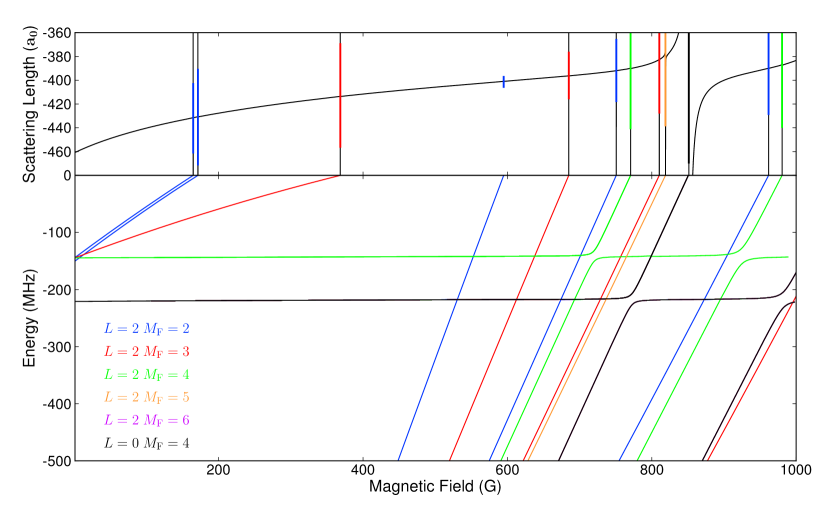
Figure 1: (Color online) Upper panel: The calculated s-wave scattering length in the aa channel of ⁸⁵Rb₂, with resonances marked with lines whose color depends on their $M_{F}$ value (see legend); the length of each line is proportional to the logarithm of the width of the resonance. Lower panel: The energies of weakly bound molecular states, relative to the aa threshold, $(2,+2)+(2,+2)$ channel. All calculations in this figure are for $M_{\rm{tot}}=4$, corresponding to s-wave scattering in the aa channel.

II Theory

The collision Hamiltonian for a pair of alkali-metal atoms is

$$\frac{\hbar^{2}}{2\mu}\bigg{[}-r^{-1}\frac{d^{2}}{dr^{2}}r+\frac{\hat{L}^{2}}{r^{2}}\bigg{]}+\hat{H}_{\rm{1}}+\hat{H}_{\rm{2}}+\hat{V}(r),$$ (1)

where $r$ is the internuclear distance, $\mu$ is the reduced mass, $\hat{L}$ is the rotational angular momentum operator and $\hat{V}$ is the interaction operator. $\hat{H}_{1}$ and $\hat{H}_{2}$ are the monomer Hamiltonians of the free atoms,

$$\hat{H}_{i}=\zeta_{i}\hat{i}_{i}\cdot\hat{s}_{i}+(g_{\rm{e}}\mu_{\rm{B}}\hat{s}_{iz}+g_{\rm{n}}\mu_{\rm{B}}\hat{i}_{iz})B,$$ (2)

where $\zeta_{i}$ is the hyperfine coupling constant of atom $i$, $g_{\rm{e}}$ and $g_{\rm{n}}$ are the electron and nuclear g-factors, $\hat{s}$ and $\hat{i}$ are the electron and nuclear spin operators and $B$ is the magnetic field.

The calculations in the present paper are carried out in two different basis sets: a fully decoupled basis set

$$\ket{s_{\rm{Rb}}m_{s\rm{Rb}}}\ket{i_{\rm{Rb}}m_{i\rm{Rb}}}\ket{s_{\rm{Rb}}m_{s\rm{Rb}}}\ket{i_{\rm{Rb}}m_{i\rm{Rb}}}\ket{LM_{L}},$$

and a partly coupled basis set

$$\ket{f_{a},m_{f,a}}\ket{f_{b},m_{f,b}}\ket{F,M_{F}}\ket{L,m_{L}}.$$

The two basis sets give identical bound-state energies and scattering properties, but different views of the bound-state wavefunctions. In both cases the basis sets are symmetrized to take account of identical particle symmetry. The resulting coupled equations are diagonal in the total projection number $M_{\rm tot}=M_{F}+M_{L}$, where $M_{F}=m_{f,a}+m_{f,b}=m_{s{\rm{Rb_{a}}}}+m_{i{\rm{Rb_{a}}}}+m_{s{\rm{Rb_{b}}}}+m_{i{\rm{Rb_{b}}}}$. The basis sets used include all functions with $L=0$ and $2$ for the required value of $M_{\rm tot}$, which for s-wave scattering is equal to $m_{f,a}+m_{f,b}$ for the incoming channel.

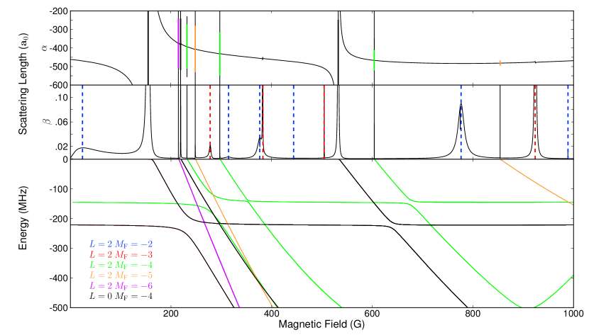
Figure 2: (Color online) Upper panels: The real and imaginary parts of the s-wave scattering length in the ee channel of ⁸⁵Rb₂. Each resonance is indicated by a colored vertical line that indicates its $M_{F}$ value (see legend); for pole-like resonances, the length of the line is proportional to the logarithm of the width of the resonance. Inelastically dominated resonances are not always evident in $\alpha$ but appear as peaks in $\beta$ and are indicated by dashed vertical lines. Lower panel: The energies of weakly bound molecular states, relative to the ee threshold, $(2,-2)+(2,-2)$ channel. Only states with no continuum interference ($M_{F}\leq-4$) are shown in the bound-state map, but all resonances are included in the scattering length. All calculations in this figure are for $M_{\rm{tot}}=-4$, corresponding s-wave scattering in ee channel.

The coupled-channel scattering calculations are performed using the MOLSCAT program Hutson and Green (1994), as modified to handle collisions in an external field González-Martínez and Hutson (2007). Calculations are carried out with a fixed-step log-derivative propagator Manolopoulos (1986) from 0.3 nm to 2.1 nm and a variable-step Airy propagator Alexander (1984) from 2.1 nm to 1,500 nm. The wavefunctions are matched to their long range solutions, the Ricatti-Bessel functions, at 1,500 nm to find the S-matrix elements. The s-wave ($L=0$) scattering length $a(k)$ is then obtained from the identity $a(k)=(ik)^{-1}(1-S_{00})/(1+S_{00})$ Hutson (2007), where $S_{00}$ is the diagonal S-matrix element in the incoming channel and $k$ is the wavevector. The bound-state calculations use the BOUND Hutson (1993) and FIELD Hutson (2011) packages, which locate bound states using as described in Ref Hutson et al. (2008). BOUND and FIELD use propagator methods, without radial basis sets. The calculations allow the assignment of quantum numbers to the states responsible for resonances in the scattering length.

The scattering and bound-state calculations are carried out using the potential curves and magnetic dipole coupling function from Ref. Strauss et al. (2010). The potentials were obtained by fitting to spectroscopic data on both the singlet Seto et al. (2000) and triplet states of ⁸⁷Rb₂ and the triplet state of ⁸⁵Rb₂, together with several Feshbach resonances in ⁸⁷Rb₂, ⁸⁷Rb⁸⁵Rb and ⁸⁵Rb₂. The singlet and triplet scattering lengths for ⁸⁵Rb on the potentials of ref. Strauss et al. (2010) are $a_{S}=2735$ $a_{0}$ and $a_{T}=-386$ $a_{0}$ respectively.

The calculated s-wave scattering length for the aa channel is shown in the top panel of Figure 1 and the binding energies of the near-threshold molecular states responsible for the resonances are shown in the lower panel. The resonance positions are given in Table 1, along with their widths $\Delta$ as defined by local fits to the standard formula $a(B)=a_{\rm{bg}}\left[1-\Delta/(B-B_{0})\right]$ Moerdijk et al. (1995), where $a_{\rm bg}$ is the background scattering length, $\Delta$ is the width, and $B_{0}$ is the position of the pole in the scattering length. Quantum numbers were assigned by carrying out approximate calculations with either $M_{F}$ or $F$ and $M_{F}$ restricted to specific values. For a homonuclear diatomic molecule, $F$ is a nearly good quantum number in the low-field region where the free-atom energies vary linearly with $B$. Figure 1 shows one wide resonance near 851 G ($\Delta=1.2$ G) that offers attractive possibilities for precise tuning of the scattering length, and many narrower resonances that may be useful for molecule formation.

For an excited-state channel, where inelastic scattering can occur, the scattering length $a(B)$ is complex, $a(B)=\alpha(B)-i\beta(B)$. The two-body inelastic loss rate is proportional to $\beta(B)$. The upper panels of Figure 2 show the real and imaginary parts of $a(B)$ for s-wave collisions in the ee channel. In this case the inelastic collisions produce atoms in lower magnetic sublevels, with $m_{f,a}$ and/or $m_{f,b}>-2$. The lower panel shows the corresponding molecular bound states for $M_{F}=-4$, $-5$ and $-6$, obtained from calculations with $M_{F}$ fixed. We also carried out calculations of the quasibound states with $M_{F}=-2$ and $-3$ near the ee threshold in order to identify the states responsible for the remaining resonances. These calculations use the FIELD program with propagation to reduced distances around 100 nm in order to reduce interference from continuum states.

In the presence of inelastic scattering, $a(B)$ does not show actual poles at resonance Hutson (2007). If the background inelastic scattering is negligible, the real part $\alpha(B)$ shows an oscillation of amplitude $a_{\rm res}$, while the imaginary part shows a peak of height $a_{\rm res}$. The resonant scattering length $a_{\rm res}$ is determined by the ratio of the couplings from the quasibound state responsible for the resonance to the incoming and inelastic channels Hutson (2007). If there is significant background scattering, then there is a more complicated asymmetric lineshape that may show a substantial dip in the inelastic scattering near resonance Hutson et al. (2009). Figure 2 shows resonances of all these different types: the resonances due to bound states with $M_{F}=m_{f,a}+m_{f,b}=-4$, $-5$ and $-6$ are pole-like, with values of at least $a_{\rm res}>20$ $a_{0}$ and with most $a_{\rm res}>1000$ $a_{0}$. These resonances produce pronounced features in $\alpha(B)$ and sharp peaks in $\beta(B)$, off scale in Figure 2. By contrast, resonances due to states with $M_{F}=-2$ and $-3$ show much weaker features with $a_{\rm res}<15$ $a_{0}$ and some lower than 0.01 $a_{0}$. These are barely perceptible in $\alpha(B)$ on the scale of Figure 2 and produce broader, weaker peaks in $\beta(B)$. The distinction occurs because all the inelastic channels have $M_{F}>-4$: bound states with $M_{F}=-2$ and $-3$ are generally more strongly coupled to inelastic channels with the same $M_{F}$ than to the incoming channel with $M_{F}=-4$, whereas the reverse is true for bound states with $M_{F}=-4$, $-5$ and $-6$. Many of the features show quite pronounced asymmetry in the shape of the inelastic peaks. All of the resonances with $a_{\rm res}>1.0$ $a_{0}$ are listed in Table 2 along with their widths and approximate $a_{\rm res}$ values.

We have also investigated the scattering length for mixed spin channels with a view to identify broad resonances suitable for manipulating interactions. Most channels exhibit strong inelastic decay with measured trap lifetimes of $\sim 100$ ms. However, the $(2,+2)+(3,+3)$ channel is immune to inelastic spin exchange collisions, resulting in trap lifetimes of $\sim 5$ s. The scattering length in the mixed spin channel, $(2,+2)+(3,+3)$ shows two pole-like resonances at 818.8 G and 909.9 G, both with widths of $2$ mG, and $a_{\rm res}$= 1600 $a_{0}$ and 800 $a_{0}$ respectively.

III Experiment

The details of our apparatus and cooling scheme are presented in Refs. McCarron et al. (2011); Cho et al. (2011, 2012) and are only briefly recounted here. Ultracold samples of ⁸⁵Rb are collected in a magneto-optical trap before being optically pumped into the $(2,-2)$ state and loaded into a magnetic quadrupole trap. Forced RF evaporation cools the ⁸⁵Rb atoms to 50 $\mu$K where further efficient evaporation is impeded by Majorana losses Lin et al. (2009). The atoms are then transferred into a crossed dipole trap derived from a single-mode 1550 nm, 30W fibre laser. When loading, the power in each beam is set to 4 W, creating a trap 100 $\mu$K deep with radial and axial trap frequencies of 455 Hz and 90 Hz respectively. After loading, when performing Feshbach spectroscopy in the absolute internal ground state, the ⁸⁵Rb atoms are transferred into the $|2,+2\rangle$ state by RF adiabatic passage Jenkin et al. (2011). A vertical magnetic field gradient of 21.2 G/cm is then applied, slightly below the 22.4 G/cm necessary to levitate ⁸⁵Rb. In contrast, when working with the $(2,-2)$ state, no magnetic field gradient is applied and the atoms are confined in a purely optical potential.

A typical experiment begins with $6.0(3)\times 10^{5}$ ⁸⁵Rb atoms at $10.2(1)~{}\mu$K confined in the dipole trap in either $(2,+2)$ or $(2,-2)$. To perform Feshbach spectroscopy, the magnetic field is switched to a specific value in the range 0 to 1000 G. Evaporative cooling is then performed by reducing the dipole beam powers by a factor of 4 over 2 s. The atomic sample is then held for 1 s in this final potential. Resonant absorption imaging is used to probe the atoms after each experimental cycle. Feshbach resonances are identified by examining the variation in the atom number and temperature as a function of the magnetic field. The magnetic field is calibrated using microwave spectroscopy between the hyperfine states of ⁸⁵Rb. These measurements reveal our field stability to be $0.1$ G for the range 0 to 400 G and $0.5$ G for the range 400 to 1000 G.

To perform Feshbach spectroscopy on a spin mixture of $(2,+2)+(3,+3)$, a cloud of $(2,+2)$ atoms is first cooled using the same evaporation sequence as above at 22.6 G. To populate the $(3,+3)$ state a microwave pulse is applied for 250 ms at 3.0887 GHz producing a mixture containing $7(1)\times 10^{4}$ atoms in each of the $(2,+2)$ and $(3,+3)$ spin states. The magnetic field is then switched to a value in the range 0 to 1000 G and held for 750 ms. Finally, Stern-Gerlach spectroscopy and absorption imaging are used to probe both spin states simultaneously.

IV Experimental Results

We have observed 7 resonances in the aa channel and 9 resonances in the ee channel. The observed and predicted resonance positions and widths are listed in Tables 1 and 2 and show good agreement between experiment and theory. In the ground state, all the widest calculated resonances are seen experimentally, with the exception of the two high-field resonances where the experimental field is less stable. In the excited state, all but two of the predicted pole-like resonances are seen, together with two of the inelastically dominated features.

Figure 3: Narrow resonances in ⁸⁵Rb, with fitted width $\delta<0.2$ G, observed as loss features in the atom number. (a) A resonance in the $(2,-2)$ state at 248.64(1) G. (b) A resonance in the $(2,+2)$ state at 770.81(1) G. The error bars show the standard deviation for multiple control shots at specific magnetic fields.

Figure 4: Broad resonances in ⁸⁵Rb, with width $\Delta>1$ G, observed as features in the atom number. (a) A resonance in the $(2,-2)$ state at 532.3(3) G. (b) A resonance in the $(2,+2)$ state at 852.3(3) G. The experimental widths are determined by the difference between the positions of the minima and maxima in the atom number marked with solid lines in both plots. The error bars show the standard deviation for multiple control shots at specific magnetic fields.

Figure 3 shows fine scans of the atom number for two of the narrow resonances, one in each of the aa and ee channels. Such resonances produce sharp drops in atom number. The experimental positions and widths of these resonances are determined by fitting a Lorentzian, with width $\delta$, to the data points. It should be noted that the experimental and theoretical widths are entirely different quantities for narrow resonances, and should not be compared.

Figure 5: The two inelastically dominated features observed in the $(2,-2)$ state. Figures (a) and (b) show the atom number while (c) and (d) show temperature. Error bars show the standard deviation for multiple control shots at specific magnetic fields. (e) and (f) show the calculated rate coefficient for two-body loss $K_{\rm loss}$.

There are three resonances with widths greater than 1 G. Figure 4 shows a fine scan across the resonances near 530 G in the ee channel, and 850 G in the aa channel. In these cases the atom number shows both a peak and a trough. The trough (loss maximum) again corresponds to the resonance position, while the peak (loss minimum) occurs near the zero-crossing of the scattering length. The three wide resonances are several orders of magnitude wider than any of the other resonances seen and provide valuable control over the scattering length. Note that our measurement of the position of the well-known 155 G resonance in the ee channel is not as accurate as the determination from bound-state spectroscopy Claussen et al. (2003).

Incoming s-wave (2,2)+(2,2) state
Experiment			Theory
$B_{0}$	$\delta$		Assignment				$B_{0}$	$\Delta$	$a_{\rm{bg}}$
(G)	(G)		$L$	($f_{a}$,$f_{b}$)	$F$	$M_{F}$	(G)	(mG)	(bohr)
164.74(1)	0.08(2)		2	(2,2)	4	2	164.7	$-0.0006$	$-432$
171.36(1)	0.12(2)		2	(2,2)	2	2	171.3	$-0.02$	$-431$
368.78(4)	0.4(1)		2	(2,2)	4	3	368.5	$-0.06$	$-413$
-	-		2	(2,3)	3	2	594.9	$-0.4\times 10^{-6}$	$-401$
-	-		2	(2,3)	5	3	685.0	$-0.4\times 10^{-4}$	$-396$
-	-		2	(2,3)	5	2	750.8	$-0.0003$	$-392$
770.81(1)	0.11(2)		2	(2,3)	5	4	770.7	$-0.5$	$-390$
809.65(3)	0.3(1)		2	(2,3)	3	3	809.7	$-0.09$	$-383$
819.8(2)	1.1(5)		2	(2,3)	5	5	819.0	$-5.4$	$-380$
852.3(3)	1.3(4)†		0	(2,3)	5	4	851.3	$-1199$	$-393$
-	-		2	(2,3)	2	2	961.8	$-0.01$	$-390$
-	-		2	(2,3)	4	4	980.5	$-0.7$	$-387$

Table 1: Location and assignment of Feshbach resonances for ⁸⁵Rb₂ in the aa channel in the field range between 0 and 1000 G. All quantum numbers in the table refer to the molecular states. The experimental errors shown are statistical uncertainties resulting from the fits as described in the text. The experimental width labeled ^† was determined from the difference between the minima and maxima in the measured atom number. Additional systematic uncertainties of $0.1$ G and $0.5$ G apply to resonance positions in the field ranges 0 to 400 G and 400 to 1000 G respectively.

Incoming s-wave (2,$-2$)+(2,$-2$) state
Experiment			Theory
$B_{0}$	$\delta$		Assignment		$B_{0}$	$\Delta$	$a_{\rm{res}}$	$a_{\rm{bg}}$
(G)	(G)		$L$	$M_{F}$	(G)	(mG)	(bohr)	(bohr)
156(1)	10.5(5)		0	$-4$	155.3	10900	$\geq$10000	$-441$
-	-		2	$-6$	215.5	5.5	4000	$-374$
219.58(1)	0.22(9)		0	$-4$	219.9	9.1	4000	$-379$
232.25(1)	0.23(1)		2	$-4$	232.5	2.0	400	$-393$
248.64(1)	0.12(2)		2	$-5$	248.9	2.9	5000	$-406$
297.42(1)	0.09(1)		2	$-4$	297.7	1.8	5000	$-432$
382.36(2)	0.19(1)		2	$-3$	382	-	15	$-457$
532.3(3)	3.2(1)†		0	$-4$	532.9	2300	$\geq$10000	$-474$
604.1(1)	0.2(1)		2	$-4$	604.4	0.03	700	$-466$
-	-		2	$-5$	854.3	0.002	25	$-481$
924.52(4)	2.8(1)		2	$-3$	924	-	9	$-476$

Table 2: Location and assignment of Feshbach resonances for ⁸⁵Rb₂ in the ee channel in the field range between 0 and 1000 G. All resonances shown satisfy $a_{\rm{res}}\geq 1$ $a_{0}$. All quantum numbers in the table refer to the molecular states. The experimental errors shown are statistical uncertainties resulting from the fits as described in the text. The experimental width labeled ^† was determined from the difference between the minima and maxima in the measured atom number. Additional systematic uncertainties of 0.1 G and 0.5 G apply to resonance positions in the field ranges 0 to 400 G and 400 to 1000 G respectively. The resonances near 155 G and 220 G have been measured previously Claussen et al. (2003); Altin et al. (2010).

The two inelastically dominated features that are seen experimentally are those with the largest $a_{\rm res}$ values. The number of atoms in the trap decreases around these resonances due to an increase in the 2-body loss rate, as shown in Figure 5(a) and (b). The inelastic collisions also lead to an increase in temperature, as shown in Figure 5 (c) and (d). The rate coefficient for 2-body losses due to inelastic collisions from a channel $n$ is

$$K^{(2)}_{\rm loss}(B)=\frac{2h}{\mu}g_{n}\beta(B),$$ (3)

where $\beta(B)$ is the imaginary part of the scattering length and $g_{n}=2$ for a thermal cloud of identical bosons Chin et al. (2010). The calculated rate coefficients for the two resonances are shown in panels (e) and (f); they peak around $1\times 10^{-11}$ cm³/s, which is an order of magnitude higher than for any of the other inelastically dominated features.

We have also measured one resonance in the $(2,+2)+(3,+3)$ mixed spin channel. The experimental results are presented in Figure 6 where a loss feature in the ⁸⁵Rb $(2,+2)$ number reveals the location of the resonance. A Lorentzian fit gives a resonance position of 817.45(5) G and an experimental width of 0.031(1) G, which may be compared with the predicted position 818.8 G.

Figure 6: A resonance measured between the $(2,+2)$ and $(3,+3)$ spin states in ⁸⁵Rb at 817.45(5) G. On resonance the increased inelastic collision rate in the mixture results in a loss feature in the $(2,+2)$ atom number as a function of magnetic field. The error bars show the standard deviation for multiple control shots at a specific magnetic field.

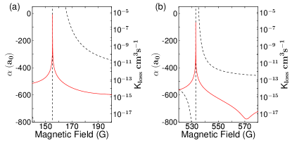
Figure 7: The rate coefficient for 2-body loss $K_{\rm loss}$ (red solid lines), which is proportional to the imaginary part of the scattering length, and the corresponding real part of the scattering length (dashed lines) for the two resonances with $\Delta>1$ G in the ee channel. Note the dip in $K_{\rm loss}$ on the high-field side the 532 G resonance.

V Conclusion

A detailed understanding of the two-body scattering behavior is essential for understanding many phenomena in ultracold gases. These include studies of molecule formation Donley et al. (2002); Thompson et al. (2005); Köhler et al. (2005); Hodby et al. (2005); Brown et al. (2006), Efimov states and their universality Stoll and Köhler (2005); Altin et al. (2011); Wild et al. (2012); Berninger et al. (2011), dimer collisions and few-body physics Ferlaino et al. (2008), BEC production Cornish et al. (2000); Weber et al. (2003), controlled condensate collapse Roberts et al. (2001a); Donley et al. (2001); Altin et al. (2011), and the formation of bright matter wave solitons Cornish et al. (2006). The scattering properties of many alkali-metal atoms have been documented in the literature Chin et al. (2010). However, nearly all previous work on ⁸⁵Rb has focussed on a single broad resonance near 155 G. This paper redresses this balance by presenting a detailed study of the scattering properties of ⁸⁵Rb, revealing additional broad resonances and numerous unreported narrow resonances in both the ee and aa channels. As has been the case for other alkali-metal atoms, this work will facilitate many future studies using ⁸⁵Rb.

We have recently explored interspecies Feshbach resonances in mixtures of ⁸⁵Rb and ¹³³Cs Cho et al. (2012), as a key step towards the production of ⁸⁵Rb¹³³Cs molecules. The improved understanding of the collisional behavior of ⁸⁵Rb resulting from the present work is essential for the production of the high phase-space density mixtures required for efficient molecule formation. In particular, the two previously unmeasured broad resonances presented here offer new magnetic field regions for evaporative cooling. The elastic to inelastic collision ratio in the vicinity of these features is potentially more favorable for evaporative cooling than near the 155 G resonance, where direct evaporation of ⁸⁵Rb to BEC is possible Cornish et al. (2000); Marchant et al. (2012). Figure 7 compares the scattering properties around the 532 G resonance with those near the 155 G resonance. The results for the 562 G resonance show a pronounced dip in the rate coefficient for 2-body loss near 570 G, due to interference between the resonant and background contributions to the inelastic scattering Hutson (2007); Hutson et al. (2009), which offers a range of magnetic fields where more efficient cooling may be possible. No such dip in the 2-body loss rate is present near the 155 G resonance. Alternatively, the aa channel offers the prospect of evaporative cooling free from two-body loss. Although the background scattering length is moderately large and negative for ground-state atoms (see Figure 1), the broad resonance at 851 G may be used to tune the scattering length to modest positive values, improving the evaporation efficiency and offering the prospect of BEC formation directly in absolute ground state. In the future we will investigate evaporative cooling in these new field regions. We will also use the improved knowledge of the scattering of ⁸⁵Rb presented in this paper, together with similar knowledge for ¹³³Cs Chin et al. (2004); Berninger et al. (2012), to devise a route to cooling ⁸⁵Rb-¹³³Cs mixtures to suitable phase-space densities for magneto-association using a narrow interspecies resonance Cho et al. (2012).

VI Acknowledgements

We thank Paul S. Julienne for many valuable discussions. This work was supported by EPSRC and by EOARD Grant FA8655-10-1-3033. CLB is supported by a Doctoral Fellowship from Durham University.

References

- Carr et al. (2009) L. D. Carr, D. DeMille, R. V. Krems, and J. Ye, New J. Phys. 11, 055049 (2009).
- Krems (2005) R. V. Krems, Int. Rev. Phys. Chem. 24, 99 (2005).
- Chin et al. (2010) C. Chin, R. Grimm, E. Tiesinga, and P. S. Julienne, Rev. Mod. Phys. 82, 1225 (2010).
- Damski et al. (2003) B. Damski, L. Santos, E. Tiemann, M. Lewenstein, S. Kotochigova, P. Julienne, and P. Zoller, Phys. Rev. Lett. 90, 110401 (2003).
- Ni et al. (2008) K.-K. Ni, S. Ospelkaus, M. H. G. de Miranda, A. Pe’er, B. Neyenhuis, J. J. Zirbel, S. Kotochigova, P. S. Julienne, D. S. Jin, and J. Ye, Science 322, 231 (2008).
- Lang et al. (2008) F. Lang, K. Winkler, C. Strauss, R. Grimm, and J. Hecker Denschlag, Phys. Rev. Lett. 101, 133005 (2008).
- Danzl et al. (2010) J. G. Danzl, M. J. Mark, E. Haller, M. Gustavsson, R. Hart, J. Aldegunde, J. M. Hutson, and H.-C. Nägerl, Nature Phys. 6, 265 (2010).
- Burke et al. (1998) J. P. Burke, J. L. Bohn, B. D. Esry, and C. H. Greene, Phys. Rev. Lett. 80, 2097 (1998).
- Cornish et al. (2000) S. L. Cornish, N. R. Claussen, J. L. Roberts, E. A. Cornell, and C. E. Wieman, Phys. Rev. Lett. 85, 1795 (2000).
- Cho et al. (2012) H.-W. Cho, D. J. McCarron, M. P. Köppinger, D. L. Jenkin, K. L. Butler, P. S. Julienne, C. L. Blackley, C. R. Le Sueur, J. M. Hutson, and S. L. Cornish, arXiv:1208.4569 (2012).
- Vogels et al. (1997) J. M. Vogels, C. C. Tsai, R. S. Freeland, S. J. J. M. F. Kokkelmans, B. J. Verhaar, and D. J. Heinzen, Phys. Rev. A 56, R1067 (1997).
- Roberts et al. (2001a) J. L. Roberts, N. R. Claussen, S. L. Cornish, E. A. Donley, E. A. Cornell, and C. E. Wieman, Phys. Rev. Lett. 86, 4211 (2001a).
- Donley et al. (2001) E. A. Donley, N. R. Claussen, S. L. Cornish, J. L. Roberts, E. A. Cornell, and C. E. Wieman, Nature 412, 295 (2001).
- Altin et al. (2011) P. A. Altin, G. R. Dennis, G. D. McDonald, D. Döring, J. E. Debs, J. D. Close, C. M. Savage, and N. P. Robins, Phys. Rev. A 84, 033632 (2011).
- Cornish et al. (2006) S. L. Cornish, S. T. Thompson, and C. E. Wieman, Phys. Rev. Lett. 96, 170401 (2006).
- Wild et al. (2012) R. J. Wild, P. Makotyn, J. M. Pino, E. A. Cornell, and D. S. Jin, Phys. Rev. Lett. 108, 145305 (2012).
- Tsai et al. (1997) C. C. Tsai, R. S. Freeland, J. M. Vogels, H. M. J. M. Boesten, B. J. Verhaar, and D. J. Heinzen, Phys. Rev. Lett. 79, 1245 (1997).
- Courteille et al. (1998) P. Courteille, R. S. Freeland, D. J. Heinzen, F. A. van Abeelen, and B. J. Verhaar, Phys. Rev. Lett. 81, 69 (1998).
- Roberts et al. (2000) J. L. Roberts, N. R. Claussen, S. L. Cornish, and C. E. Wieman, Phys. Rev. Lett. 85, 728 (2000).
- Roberts et al. (2001b) J. L. Roberts, J. P. Burke, N. R. Claussen, S. L. Cornish, E. A. Donley, and C. E. Wieman, Phys. Rev. A 64, 024702 (2001b).
- Claussen et al. (2003) N. R. Claussen, S. J. J. M. F. Kokkelmans, S. T. Thompson, E. A. Donley, E. Hodby, and C. E. Wieman, Phys. Rev. A 67, 060701 (2003).
- Donley et al. (2002) E. A. Donley, N. R. Claussen, S. T. Thompson, and C. E. Wieman, Nature 417, 529 (2002).
- Thompson et al. (2005) S. T. Thompson, E. Hodby, and C. E. Wieman, Phys. Rev. Lett. 95, 190404 (2005).
- Köhler et al. (2005) T. Köhler, E. Tiesinga, and P. S. Julienne, Phys. Rev. Lett. 94, 020402 (2005).
- Hodby et al. (2005) E. Hodby, S. T. Thompson, C. A. Regal, M. Greiner, A. C. Wilson, D. S. Jin, E. A. Cornell, and C. E. Wieman, Phys. Rev. Lett. 94, 120402 (2005).
- Brown et al. (2006) B. L. Brown, A. J. Dicks, and I. A. Walmsley, Phys. Rev. Lett. 96, 173002 (2006).
- Stoll and Köhler (2005) M. Stoll and T. Köhler, Phys. Rev. A 72, 022714 (2005).
- Hutson and Green (1994) J. M. Hutson and S. Green, “MOLSCAT computer program, version 14,” distributed by Collaborative Computational Project No. 6 of the UK Engineering and Physical Sciences Research Council (1994).
- González-Martínez and Hutson (2007) M. L. González-Martínez and J. M. Hutson, Phys. Rev. A 75, 022702 (2007).
- Manolopoulos (1986) D. E. Manolopoulos, J. Chem. Phys. 85, 6425 (1986).
- Alexander (1984) M. H. Alexander, J. Chem. Phys. 81, 4510 (1984).
- Hutson (2007) J. M. Hutson, New J. Phys. 9, 152 (2007).
- Hutson (1993) J. M. Hutson, “BOUND computer program, version 5,” distributed by Collaborative Computational Project No. 6 of the UK Engineering and Physical Sciences Research Council (1993).
- Hutson (2011) J. M. Hutson, “FIELD computer program, version 1,” (2011).
- Hutson et al. (2008) J. M. Hutson, E. Tiesinga, and P. S. Julienne, Phys. Rev. A 78, 052703 (2008).
- Strauss et al. (2010) C. Strauss, T. Takekoshi, F. Lang, K. Winkler, R. Grimm, J. Hecker Denschlag, and E. Tiemann, Phys. Rev. A 82, 052514 (2010).
- Seto et al. (2000) J. Y. Seto, R. J. Le Roy, J. Vergès, and C. Amiot, J. Chem. Phys 113, 3067 (2000).
- Moerdijk et al. (1995) A. J. Moerdijk, B. J. Verhaar, and A. Axelsson, Phys. Rev. A 51, 4852 (1995).
- Hutson et al. (2009) J. M. Hutson, M. Beyene, and M. L. González-Martínez, Phys. Rev. Lett. 103, 163201 (2009).
- McCarron et al. (2011) D. J. McCarron, H. W. Cho, D. L. Jenkin, M. P. Köppinger, and S. L. Cornish, Phys. Rev. A 84, 011603 (2011).
- Cho et al. (2011) H. W. Cho, D. J. McCarron, D. L. Jenkin, M. P. Köppinger, and S. L. Cornish, Eur. Phys. J. D 65, 125 (2011).
- Lin et al. (2009) Y.-J. Lin, A. R. Perry, R. L. Compton, I. B. Spielman, and J. V. Porto, Phys. Rev. A 79, 063631 (2009).
- Jenkin et al. (2011) D. L. Jenkin, D. J. McCarron, M. P. Köppinger, H. W. Cho, S. A. Hopkins, and S. L. Cornish, Eur. Phys. J. D 65, 11 (2011).
- Altin et al. (2010) P. A. Altin, N. P. Robins, R. Poldy, J. E. Debs, D. Döring, C. Figl, and J. D. Close, Phys. Rev. A 81, 012713 (2010).
- Berninger et al. (2011) M. Berninger, A. Zenesini, B. Huang, W. Harm, H.-C. Nägerl, F. Ferlaino, R. Grimm, P. S. Julienne, and J. M. Hutson, Phys. Rev. Lett. 107, 120401 (2011).
- Ferlaino et al. (2008) F. Ferlaino, S. Knoop, M. Mark, M. Berninger, H. Schöbel, H.-C. Nägerl, and R. Grimm, Phys. Rev. Lett. 101, 023201 (2008).
- Weber et al. (2003) T. Weber, J. Herbig, M. Mark, H.-C. Nägerl, and R. Grimm, Science 299, 232 (2003).
- Marchant et al. (2012) A. L. Marchant, S. Händel, S. A. Hopkins, T. P. Wiles, and S. L. Cornish, Phys. Rev. A 85, 053647 (2012).
- Chin et al. (2004) C. Chin, V. Vuletić, A. J. Kerman, S. Chu, E. Tiesinga, P. J. Leo, and C. J. Williams, Phys. Rev. A 70, 032701 (2004).
- Berninger et al. (2012) M. Berninger, A. Zenesini, B. Huang, W. Harm, H.-C. Nägerl, F. Ferlaino, R. Grimm, P. S. Julienne, and J. M. Hutson, arXiv , 2012:12xx (2012).