On the Impact of Phase Noise on Active Cancellation in Wireless Full-Duplex

Abstract

Recent experimental results have shown that full-duplex communication is possible for short-range communications. However, extending full-duplex to long-range communication remains a challenge, primarily due to residual self-interference even with a combination of passive suppression and active cancellation methods. In this paper, we investigate the root cause of performance bottlenecks in current full-duplex systems. We first classify all known full-duplex architectures based on how they compute their cancelling signal and where the cancelling signal is injected to cancel self-interference. Based on the classification, we analytically explain several published experimental results. The key bottleneck in current systems turns out to be the phase noise in the local oscillators in the transmit and receive chain of the full-duplex node. As a key by-product of our analysis, we propose signal models for wideband and MIMO full-duplex systems, capturing all the salient design parameters, and thus allowing future analytical development of advanced coding and signal design for full-duplex systems.

I Introduction

In full-duplex communication, a node can simultaneously transmit one signal and receive another signal on the same frequency band. The key challenge in full-duplex communications is the self-interference, which is the transmitted signal being added to the receive path of the same node. Due to the proximity of the transmit and receive antennas on a node, self-interference is often many orders of magnitude larger than the signal of interest. Thus, the main objective for full-duplex design is to reduce the strength of self-interference as much as possible – ideally, down to noise floor.

Self-interference is usually reduced by a combination of passive and active methods [2, 3, 4, 5, 6, 7, 8, 9, 10, 11]. Passive methods, which use antenna designs, aim to increase the pathloss for the self-interference signal. In contrast, active methods employ the knowledge of self-interference to cancel it from the received signal. However, none of the designs [3, 5, 6, 7, 8, 9, 4, 2, 10, 11] manage to eliminate self-interference completely. In fact, in [10], authors report that even after passive suppression and active cancellation, the strength of self-interference is 15 dB above the thermal noise floor. Our main focus, in this paper, is to understand the bottlenecks that limit self-interference from being completely eliminated in current full-duplex systems by answering the following three questions, observed experimentally in prior works.

Question 1: Active cancellation can occur before or after analog-to-digital conversion. If active cancellation occurs prior to digitization of the received signal, it is referred to as active analog cancellation. The cancellation that operates on the received signal in digital baseband is labeled digital cancellation. Designs [3, 5, 6, 8] report anywhere between 20-45 dB of active analog cancellation, which raises the first question that we answer analytically in this paper “What limits the amount of active analog cancellation in a full-duplex system design?”

Question 2: An interesting observation reported in [10] is that if active analog cancellation and digital cancellation are cascaded together, then the amount of digital cancellation depends on the amount of analog cancellation. More specifically, [10] reports that whenever their analog canceller cancels less self-interference, then the digital canceller cancels more and vice versa. The above observation leads to the second question which we answer, “How do the amounts of cancellations by active analog and digital cancellers depend on each other in a cascaded system?”

Question 3: Finally, in [10], it is also reported that more passive suppression results in increased total self-interference reduction, when both passive suppression and active analog cancellation are used. However, the total reduction does not increase linearly with amount of passive suppression. We make preliminary progress towards answering the third question, “How and when does passive suppression impact the amount of active analog cancellation?”

In this paper, we answer all the three questions using the following procedure. First, we harmonize all known architectures of active analog cancellers by classifying them into two classes: pre-mixer and post-mixer cancellers, based on where the cancelling signal is generated. Pre-mixer canceller [5] generates the cancelling signal prior to upconversion in the digital baseband, while post-mixer canceller [3, 6, 8] generates the self-interference signal at the carrier frequency. Both pre- and post-mixer perform the cancellation at the carrier frequency. As a side result, our classification yields another active analog canceller architecture which we label as baseband analog canceller. In baseband analog cancellation, both the cancelling signal as well as cancellation operation is in the analog baseband. The above classification of analog cancellers allows us to study all architectures systematically using one umbrella analysis, and thus allows direct comparisons between performance of different cancellers.

Once we classify the known architectures of full-duplex designs, we show that phase noise [12] associated with local oscillators at the transmitter and receiver turns out to be the source of major bottleneck in full-duplex systems. In fact, phase noise answers all three questions raised above. To answer Question 1, we analyze the amount of active analog cancellation possible in different types of cancellers and show that by incorporating phase noise into the signal model, we can closely match the cancellation number reported in [5] and conjecture that phase noise also explains results of [6, 8].

To answer Question 2, we show that the amount of active analog cancellation and concatenated digital cancellation is limited by a quantity that depends on the phase noise properties of the local oscillators. We show that, if the active analog canceller cancels more, the residual self-interference has a dominant contribution of phase noise, which is uncorrelated to the self-interference signal and thus cannot be cancelled by the concatenated digital canceller. On the other hand, if active analog canceller cancels less, the residual self-interference has a higher correlation to the self-interference signal and thus a larger fraction of self-interference can be cancelled by the digital canceller.

To answer Question 3, we show that due to phase noise the amount of active analog cancellation, in a pre-mixer canceller, is dependent on the amount of passive suppression. We show that the sum total of passive suppression and active analog cancellation increases with an increase in passive suppression, but individually the amount of active analog cancellation reduces as the amount of passive suppression increases. As a result, the sum total of passive suppression and active cancellation does not increase linearly with increase in passive suppression.

Finally, as a by-product of our analysis of active cancellers, we propose signal models for MIMO and wideband full-duplex systems. The signal models allow us to abstract away the form of active cancellation, and can be used for signal design and analysis of full-duplex systems. The noise term in the proposed signal model depends on three parameters: phase noise variance and its autocorrelation, quality of self-interference channel estimates and thermal noise. Each of the three parameters decides the dominant noise in full-duplex system in different regimes of transmitted self-interference power, thus captures the limits of communication in full-duplex.

The rest of the paper is organized as follows. In Section II, we review the need for active cancellation and classify the different known architectures of active analog cancellers. In Section III, we show that self-interference channel estimation error does not explain the amount of active analog cancellation reported in literature [5, 3, 6, 8]. In Section IV, via a controlled experiment, we show that phase noise limits the amount of active cancellation. In Section V and VI, we analyse the amount of active analog cancellation and concatenated digital cancellation possible in different cancellers, uncovering their interdependence. In Section VII, we show the interdependence between passive suppression and active cancellation for pre-mixer cancellers. Finally, in Section VIII we propose the MIMO and wideband signal model for full-duplex systems. We conclude in Section IX.

II Reducing Self-Interference in Full-Duplex

II-A Need for self-interference reduction

Due to simultaneous transmission and reception in full-duplex, a combination of incoming signal of interest and self-interference is received at the full-duplex node. Since the transmit and receive antenna at the full-duplex node are in physical proximity, the self-interference signal can be 50-100 dB larger in magnitude compared to the signal of interest. For baseband processing, the received signal is digitized using an analog to digital convertor, which has a finite number of bits of quantization. Before digitizing the signal, the automatic gain control scales the input to a nominal range of $[-1,1]$. Since the signal of interest is weaker than the self-interference, the gain control settings are largely governed by the strength of the self-interference, leading to the signal of interest occupying a range much smaller than $[-1,1]$ in the quantized signal. After digitization, even if the self-interference signal can be perfectly subtracted out, the quantization noise for the signal of interest will be significantly large, leading to a very low effective SNR in digital baseband. Thus, it is important to reduce the self-interference prior to analog to digital conversion, so that the signal of interest will have a better effective SNR in digital baseband.

II-B Methods of reducing self-interference

Self-interference is reduced by both passive and active techniques. A diagramatic classification of methods of reducing self-interference is shown in Figure 2. A figure of merit to characterize any technique used to reduce self-interference is the ratio of the strength of self-interference before and after the technique is employed, which is called the amount of suppression for passive and cancellation for active techniques. Following is a brief review of the methods to reduce self-interference.

II-B1 Passive suppression

Passive suppression aims to reduce the self-interference by reducing the electromagnetic coupling between the transmit and receive antenna at the full-duplex node. As shown in Figure 2, the reduction in the strength of self-interference via passive methods occurs before the self-interference signal impinges upon the receive antenna. Passive methods include (a) antenna-separation, which achieves reduction of the self-interference by increasing pathloss between transmit and receive antenna [7, 5, 3], (b) directional-separation, where the transmit and receive antenna on the full-duplex node have lower mutual coupling as the main lobes of the antennas do not point to each other [13, 14], (c) polarization decoupling [14], where the transmit and receive antenna operate on orthogonal polarizations to reduce the coupling.

II-B2 Active analog cancellation

The mechanism of reducing self-interference which employs the knowledge of self-interference to actively inject a cancelling signal into the received signal in the analog domain is referred to as active analog cancellation. As shown in Figure 2, active analog cancellation operates on the received signal. Thus, active analog cancellation occurs after passive suppression. The objective of active analog cancellation is to create a null for the self-interference signal. The null for self-interference can be created by performing cancellation either at the carrier frequency (RF) or at the analog baseband. Most active analog cancellers [3, 5, 6, 8] cancel self-interference at RF. We first classify active analog cancellers which cancel at RF and then describe the canceller which cancel in analog baseband.

Active analog cancellation at RF

In Figure 3(a), we depict a block diagram of an active analog canceller which cancels at RF. Note that, if the cancellation has to be performed at RF, then the cancelling signal also needs to be upconverted to RF. The cancelling signal is generated by processing the self-interference signal $x_{\sf si}(t)$. We classify active analog cancellers based on whether the cancelling signal has been generated by processing the self-interference signal $x_{\sf si}(t)$, prior or post upconversion. Those cancellers where the cancelling signal is generated by processing $x_{\sf si}(t)$ prior to upconversion are called pre-mixer cancellers, while cancellers where the cancelling signal is generated by processing after $x_{\sf si}(t)$ is upconverted are called post-mixer cancellers. Figure 3(a) shows the pre-mixer processing function $f(.)$ and post-mixer processing function $g(.)$. The choice of functions $f(.)$ and $g(.)$ are ideal if after cancellation the self-interference signal is completely eliminated from the received signal. For many known implementations, we show the choice of functions $f(.)$ and $g(.)$ classify them as pre- and post-mixer cancellers as follows.

Parallel radio cancellation: In [5], the negative of the scaled self-interference signal being received at the receiver of the full-duplex node is generated in the digital baseband and unconverted via a parallel radio chain. The cancelling signal is then added to the received signal at carrier frequency using a passive power combiner. The functions

$$f(t)=h(t);g(t)=\delta(t),$$ (1)

are implemented as filters, where $h(t)$ is a filter that is implemented in digital domain. To cancel the self-interference, the design implements $h(t)=-\hat{h}_{\sf si}(t)$, where $\hat{h}_{\sf si}(t)$ is the estimate of the self-interference channel $h_{\sf si}(t)$. If $\hat{h}_{\sf si}(t)=h_{\sf si}(t)$, and $\ast$ represents the convolution operation, then the cancellation should result $h_{\sf si}(t)\ast x_{\sf si}(t)-\hat{h}_{\sf si}(t)\ast x_{\sf si}(t)=(h_{\sf si}(t)-\hat{h}_{\sf si}(t))\ast x_{\sf si}(t)=0$.

BALUN cancellation: In [6], a copy of the signal in RF is passed through a BALUN which produces the negative of the analog signal being transmitted. The negative signal is then amplified and delayed using a QHX220 analog chip [15], and finally added to the received signal in the analog domain, thus cancelling the self-interference. The generation of cancelling signal as well as cancellation occurs at carrier frequency, thus we classify BALUN cancellation as post-mixer cancellation. The functions

$$f(t)=\delta(t);g(t)=-g_{1}\delta(t)-g_{2}\delta(t-\tau),$$ (2)

where $g_{1}$ and $g_{2}$ are gain coefficients and $\tau$ is a fixed delay. If the coefficients $g_{1}$ and $g_{2}$ are chosen such that $g_{1}\delta(t)+g_{2}\delta(t-\tau)=h_{\sf si}(t)$, then a null is created at the receiver.

Antenna cancellation: In [8], at the full-duplex node, two transmit antennas Tx1_a and Tx1_b are placed at equal distance symmetrically away from the receive antenna. The transmit antennas transmit signals which are negative of each other. Upon reception, the copies of self-interference signals negate each other resulting in a smaller self-interference. Antenna cancellation is an example of post-mixer canceller because the processing occurs at RF as described by the functions

$$f(t)=\delta(t);g(t)=-h_{b,{\sf si}}(t),$$ (3)

where $h_{b,{\sf si}}(t)$ is the over the air channel from antenna Tx1_b to the receive antenna. If the channel from Tx1_a to the receiver, $h_{a,{\sf si}}(t)=h_{b,{\sf si}}(t)$, then a perfect null is created at the receiver.

Note that, in all the mechanisms described above, while the cancellation is performed in RF-analog domain, the input to $f(.)$ can either be a digital or an analog signal, while the input to $g(.)$ is necessarily an analog signal.

Baseband analog canceller

An active analog canceller where the cancelling signal is generated in baseband as well as the cancellation occurs in the analog baseband is called baseband analog canceller. Figure 3(b) shows a representation of baseband analog canceller. In baseband analog cancellers the self-interference signal $x_{\mathsf{si}}(t)$ is processed by a function $s(.)$, either in baseband analog domain or in digital domain before it is added to the received signal to perform the cancellation. If the function $s(.)$ is such that the self-interference signal is negative of the cancelling signal at the receiver, then a null is created for the self-interference. Since the cancelling signal does not go through upconversion process, possibly less RF hardware is required to implement a baseband analog canceller.

II-B3 Digital cancellation

The active cancellation which occurs in the digital domain after the received signal has been quantized by an analog to digital convertor is called active digital cancellation. Examples of full-duplex systems where digital cancellation has been implemented are [5, 3]. From Figure 2, we see that digital cancellation is the final step of reduction of self-interference. digital

III First Attempt

In this section, we show that the conventional signal model for narrowband communication does not satisfactorily explain the amount of active analog cancellation reported in [3, 5, 6, 8].

III-A Narrowband Signal Model

Let $\sf N$1 denote a full-duplex node which transmits the self-interference signal $x_{\sf si}(t)$, while $\sf N$2 denote the node from which $\sf N$1 is receiving the signal of interest denoted by $x_{\sf signal}(t)$. The impulse response of the self-interference channel is denoted by $\mathbf{h_{\sf si}}(t)$, while the impulse response of channel from $\sf N$2’s transmitter to $\sf N$1’s receiver be denoted by $\mathbf{h_{\sf signal}}(t)$. Then, the received signal at $\sf N$1 denoted by $y_{1}(t)$ is given by

$$y_{1}(t)=\mathbf{h}_{\sf si}(t)\ast x_{\sf si}(t)+\mathbf{h}_{\sf signal}(t)\ast x_{\sf signal}(t)+z_{\sf noise}(t),$$ (4)

where $\ast$ denotes the convolution operation, $z_{\sf noise}(t)$ is the AWGN thermal noise distributed as $\mathcal{N}(0,\sigma_{\sf noise}^{2})$. For a narrowband signal, the wireless channel can be modeled as single tap delay channel, $\mathbf{h}_{\sf si}(t)=h_{\sf si}\delta(t-\Delta_{\sf si})$, and $\mathbf{h}_{\sf signal}(t)=h_{\sf signal}\delta(t-\Delta_{\sf signal})$. Note that $h_{\sf si}$ and $h_{\sf signal}$ are complex attenuations which depend on channel conditions, while $\Delta_{\sf si},\Delta_{\sf signal}\in\mathbb{R}^{+}$ are delays with which the self-interference signal and the signal of interest, respectively, arrive at the receiver. Note that, the signal model in (4) describes a time-invariant system. The assumption of time-invariance is valid as long we assume that (4) describes $y_{1}(t)$ within the coherence times of the channels $\mathbf{h}_{\sf si}(t)$ and $\mathbf{h}_{\sf signal}(t)$. The average power at each of the transmitters is nominally limited to 1, which implies

$$\mathbb{E}(|x_{\sf si}(t)|^{2})\leq 1,\text{ }\mathbb{E}(|x_{\sf signal}(t)|^{2})\leq 1.$$ (5)

The digital baseband equivalent of (4) can be written by replacing $t$ by $iT$ where $T$ is the sampling period and $i\in\mathbb{Z}$.

III-B Amount of cancellation

Let $\widehat{\mathbf{h}}_{\sf si}(t)=\hat{h}_{\sf si}\delta(t-\hat{\Delta}_{\sf si})$ be the estimate of the self-interference channel. With imperfect estimate of the channel, the residual self-interference after active analog cancellation will be

$$y_{1,{\sf residual}}(t)=h_{\sf si}x(t-\Delta_{\sf si})-\hat{h}_{\sf si}x(t-\hat{\Delta}_{\sf si})+z_{\sf noise}(t).$$ (6)

Equation (6) implies that when $\widehat{\mathbf{h}}_{\sf si}(t)=\mathbf{h}_{\sf si}(t)$, then the residual is only due to thermal noise. The strength of the residual self-interference is given by

$$\sigma_{\sf residual}^{2} = \mathbb{E}(|y_{1,{\sf residual}}(t)|^{2})$$

$$\stackrel{{\scriptstyle\text{(a)}}}{{=}} \mathbb{E}\left(|\hat{h}_{\sf si}x(t-\hat{\Delta}_{\sf si})-h_{\sf si}x(t-\Delta_{\sf si})|^{2}\right)+\sigma_{\sf noise}^{2}$$

$$= \mathbb{E}\left(|\hat{h}_{\sf si}(x_{\sf si}(t-\hat{\Delta}_{\sf si})-x_{\sf si}(t-\Delta_{\sf si}))+(\hat{h}_{\sf si}-h_{\sf si})x_{\sf si}(t-\Delta_{\sf si})|^{2}\right)+\sigma_{\sf noise}^{2}$$

$$\stackrel{{\scriptstyle\text{(b)}}}{{=}} 2\mathbb{E}\left(|\hat{h}_{\sf si}|^{2}\right)(1-R_{x_{\sf si}}(\hat{\Delta}_{\sf si}-\Delta_{\sf si}))+\mathbb{E}\left(|\hat{h}_{\sf si}-h_{\sf si}|^{2}\right)$$

$$+2\text{Re}\left\{\mathbb{E}\left(\hat{h}_{\sf si}(h_{\sf si}-\hat{h}_{\sf si})(x_{\sf si}(t-\hat{\Delta}_{\sf si})-x_{\sf si}(t-\Delta_{\sf si}))x_{\sf si}(t-\Delta_{\sf si})\right)\right\}+\sigma_{\sf noise}^{2},$$ (7)

where (a) holds because of independence of thermal noise with self-interference channel and the signal itself, (b) is true due to assumption that the average power at the transmitter is unity. Estimating a channel with single delay tap has been studied in [16], where it is shown that estimation error in the channel attenuation behaves as

$$\mathbb{E}\left(|\hat{h}_{\sf si}-h_{\sf si}|^{2}\right)=\frac{\sigma_{\sf noise}^{2}}{T_{\sf train}},$$ (8)

where $T_{\sf train}$ is the length of the training sequence used to estimate the self-interference channel. Also, let $h_{\sf si,error}$ denote the error in the estimate of the channel attenuation, then

$$\mathbb{E}\left(\hat{h}_{\sf si}(h_{\sf si}-\hat{h}_{\sf si}))\right) = \mathbb{E}\left((h_{\sf si,error}+h_{\sf si})h_{\sf si,error}\right)=\mathbb{E}\left((h_{\sf si,error})^{2}\right)+h_{\sf si}\mathbb{E}\left(h_{\sf si,error}\right)=\frac{\sigma_{\sf noise}^{2}}{T_{\sf train}}.$$ (9)

In [16], it has been shown that the variance in the estimate of the delay goes down as the inverse of training length $T_{\sf train}$. Moreover, it can be easily shown that for any bandlimited signal $x_{\sf si}(t)$ and small enough $\Delta_{\sf si}-\hat{\Delta}_{\sf si}$,

$$1-R_{x_{\sf si}}(\Delta_{\sf si}-\hat{\Delta}_{\sf si})\leq c(\Delta_{\sf si}-\hat{\Delta}_{\sf si})^{2},$$ (10)

where $R_{x_{\sf si}}(.)$ is the autocorrelation function of $x_{\sf si}(t)$ and $c$ is a positive constant (see Appendix X-A for details). Applying (8), (9), (10) and Equation (6) of [16] to (7), the residual self-interference for the signal model in (4) is bounded above as

$$\sigma_{\sf residual}^{2}<\frac{5\sigma_{\sf noise}^{2}}{T_{\sf train}}+\sigma_{\sf noise}^{2},$$ (11)

i.e., it decays inversely to the training length $T_{\sf train}$. Letting $T_{\sf train}\to\infty$ for (4), the residual self-interference should only be composed of thermal noise. Since the channel estimation error decays inversely to the length of the training, for the signal model described by (4), even with a very short training length, say $T_{\sf train}=5$ the residual self-interference is no more than 3 dB above thermal noise. However, the observed phenomenon in [10] is that the residual self-interference is 15 dB higher than the thermal noise which is clearly not explained by the signal model in (4). In [5, 3, 6] too the residual self-interference is reported to be much higher than 15 dB above thermal noise floor, thus we suspect that channel model in (4) does not capture all dominant sources of radio impairments.

IV Identifying the Bottleneck in Active Cancellation

IV-A Possible sources of bottleneck

Transmitter phase noise, receiver phase noise, IQ imbalance, power amplifier non-linearity and quantization noise are some of the other impairments in the transmit-receive chain at the full-duplex node which can possibly limit the amount of active analog cancellation. In [5], a 14-bit ADC is used, which delivers a signal to quantization noise ratio of 84 dB, making quantization noise much smaller than the thermal noise, thus ruling quantization noise out as a source of bottleneck in estimation of self-interference and consequently active analog cancellation. IQ imbalance does not vary significantly with time and can be easily calibrated, thus eliminating it as a source of bottleneck. Power amplifier shows significant non-linearity only when it is operated in its non-linear regime. In this paper, we want to explain the bottlenecks in current designs of full-duplex and since most of the designs to date have been designed in the linear regime of power amplifier, they do not suffer from power amplifier non-linearity.

IV-B Experiment

In our related work [1], we presented an experiment through which we identify the bottleneck in active cancellation in a full-duplex system. For the sake of completeness, we describe the steps of the experiment and then explain how it is used to identify the source of bottleneck in active cancellation. Following are the steps of the experiment, schematically shown in the Figure 4.

• A signal $x(t)=e^{j\omega t}$ is digitally generated, with $\omega/2\pi=$1MHz, and is upconverted to the carrier frequency of $f_{c}=\omega_{c}/2\pi$. Let $x_{\sf up}(t)$ denote the upconverted signal.

• The signal $x_{\sf up}(t)$ is split using a 3-port power splitter [17]. Let $x_{\sf up,1}(t)$ and $x_{\sf up,2}(t)$ denote the two signals output from the power splitter.

• Using a wired connection, the signals $x_{\sf up,1}(t)$ and $x_{\sf up,2}(t)$ are fed into two input ports of a vector signal analyzer (VSA) [18]. Using the knowledge of $\omega_{c}$, the VSA downconverts the received signals and digitizes them. Let the digitized signals, after downconversion be denoted by $y_{1}[iT]$ and $y_{2}[iT]$. In the experiment $T$ was chosen to be 21.7 ns.

The above experiment is conducted using two signal sources: an off-the-shelf radio chip [19] used in WARP [20] and a high precision Vector Signal Generator [21]. For WARP $f_{c}=\omega_{c}/2\pi=2.4$ GHz and for the Vector Signal Generator $f_{c}=\omega_{c}/2\pi=2.2$ GHz.

IV-C Mimicking active cancellation

The received signal $y_{1}[iT]$ and $y_{2}[iT]$ are sequences of complex numbers. To analyse the amount of cancellation, we treat $y_{1}[iT]$ as the self-interference signal and use a processed version of $y_{2}[iT]$ as the cancelling signal. The transmitted signal is narrowband, therefore if the upconversion process does not add any noise, then

$$y_{1}[iT] = h_{1}e^{-j(\omega_{c}+\omega)\Delta_{1}}x[iT]+z_{1}[iT],$$ (12)

$$y_{2}[iT] = h_{2}e^{-j(\omega_{c}+\omega)\Delta_{2}}x[iT]+z_{2}[iT],$$ (13)

where $h_{1}$ and $h_{2}$ are complex attenuations, and $\Delta_{1}$ and $\Delta_{2}$ are delays introduced by the wires, and $z_{1}[iT]$ and $z_{2}[iT]$ denote the thermal noise at the receiver. Using wires to connect the source and receivers ensures that the temporal variation in $h_{1}$ and $h_{2}$ is minimal. The wires are chosen of approximately the same length so that $\Delta_{1}\approx\Delta_{2}$. To mimic active cancellation, we subtract a suitably scaled version of $y_{2}[iT]$ from $y_{1}[iT]$, thereby leaving a residual self-interference which is given by

$$y_{\sf residual}[iT]=y_{1}[iT]-h_{c}y_{2}[iT],$$ (14)

where $h_{c}$ is a complex number computed as

$$h_{c} = \frac{\sum_{i=1}^{N}y_{2}[iT]^{{}^{\prime}}y_{1}[iT]}{\sum_{i=1}^{N}|y_{2}[iT]|^{2}}.$$ (15)

Now consider a delayed version of the signal $y_{2}[iT]$,

$$y_{2}[(i-d)T] = h_{2}e^{-j(\omega_{c}+\omega)\Delta_{2}}x[(i-d)T]+z_{2}[(i-d)T]$$ (16)

$$= h_{2}e^{-j((\omega_{c}+\omega)\Delta_{2}+\omega dT)}x[iT]+z_{2}[(i-d)T],$$

where $d$ is a non-negative integer. We can subtract a scaled version of $y_{2}[(i-d)T]$ from $y_{1}[iT]$ such that the residual self-interference is

$$y_{\mathsf{residual},d}[iT]=y_{1}[iT]-h_{c}(d)y_{2}[(i-d)T],$$ (17)

where the scaling $h_{c}(d)$ is computed as

$$h_{c}(d)=\frac{\sum_{i=1}^{N}y_{2}[(i-d)T]^{{}^{\prime}}y_{1}[iT]}{\sum_{i=1}^{N}|y_{2}[(i-d)T]|^{2}}.$$ (18)

If (12) and (13) hold true and if we rewrite $h_{c}(d)=\frac{h_{1}}{h_{2}}e^{j(\omega_{c}(\Delta_{2}-\Delta_{1})+\omega dT)}+\epsilon$, then the expected strength of the residual signal is given by

$$\mathbb{E}(|y_{\mathsf{residual},d}[iT]|^{2}) = \mathbb{E}(|y_{1}[iT]-h_{c}(d)y_{2}[(i-d)T]|^{2})$$ (19)

$$= |h_{2}|^{2}\mathbb{E}(|\epsilon|^{2})+\mathbb{E}(|z_{1}[iT]|^{2}+|z_{2}[(i-d)T]|^{2})=|h_{2}|^{2}\mathbb{E}(|\epsilon|^{2})+2\sigma_{\sf noise}^{2}.$$

In Appendix X-B, we show that by letting $N\to\infty$ we have

$$\mathbb{E}(|y_{\mathsf{residual},d}[iT]|^{2})=\frac{|h_{1}|^{2}}{|h_{2}|^{2}}\sigma_{\sf noise}^{2}+2\sigma_{\sf noise}^{2}.$$ (20)

For the experiment conducted $\frac{|h_{1}|^{2}}{|h_{2}|^{2}}\approx 1$, thus the strength of the residual self-interference should be approximately $3\sigma_{\sf noise}^{2}$. The analysis reveals that if (12) and (13) hold true, then the amount of cancellation should be independent of the delay $d$ and dependent only on the thermal noise.

IV-D Experiment: Results and their explanation

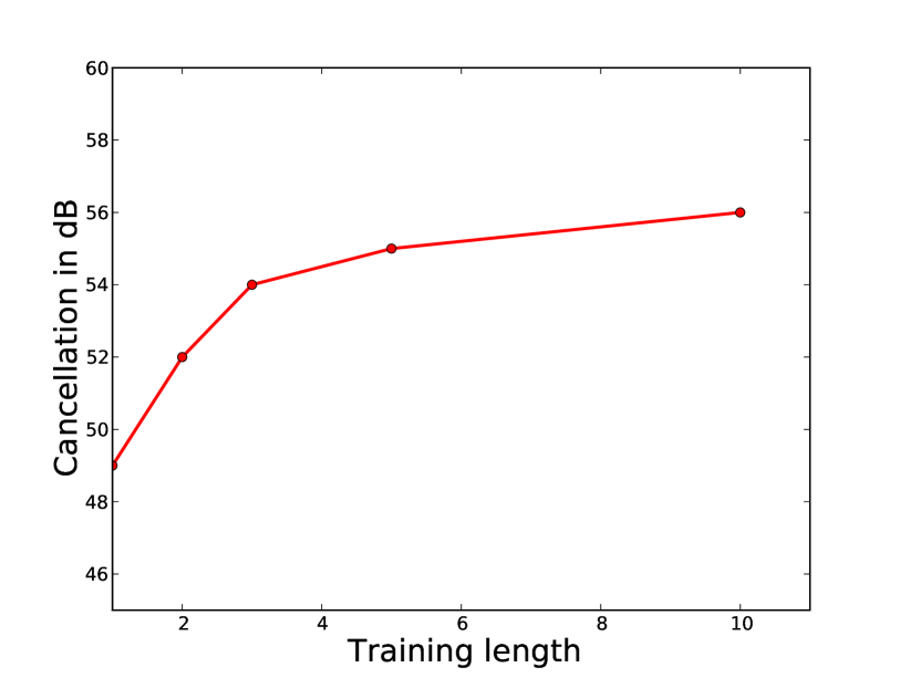
Figure 6: Amount of active cancellation as a function of the training length for a delay $d=0$ for WARP as the signal source measured from the experiment in Section IV.

In Figure 6, we plot the amount of cancellation as a function of delay $d$ measured from the experiment for both the signal sources. For WARP as the signal source, when $d$ is small then the amount of cancellation depends on the delay. As the delay increases the cancellation floors around 35 dB. The measurement from the experiment shows that for WARP as a signal source, even for a delay $d=100$, the amount of cancellation is approximately 35 dB. On the other hand, the amount of cancellation when the vector signal generator is used as a signal source is approximately 55 dB, independent of the delay.

Upper bound of cancellation

For both signal sources, the upper bound of cancellation is around 55 dB. The limitation on the cancellation can be explained by the dynamic range of the measurement equipment. The data-sheet [18] of the VSA lists that it offers a dynamic range of anywhere between 55-60 dB. Thus, the received signals $y_{1}[iT]$ and $y_{2}[iT]$ themselves have an SNR of no more 55-60 dB, thereby limiting the maximum cancellation in the range of 55-60 dB only.

Phase noise explains the trend of cancellation

Two observations from the experiment conducted, when WARP is used as a signal source source, need an explanation. The first observation is that the amount of cancellation reduces by increasing the delay between self-interference signal and cancelling signal. And the second observation is that the amount of cancellation has a lower bound of $\approx$35 dB. We claim that both the observations can be explained if we consider the perturbations introduced by phase noise in the upconverted signal.

Phase noise is the jitter in the local oscillator. If the baseband signal $x(t)$ is upconverted to a carrier frequency of $\omega_{c}$, then the upconverted signal $x_{\sf up}(t)=x(t)e^{j(\omega_{c}t+\phi(t))}$, where $\phi(t)$ represents the phase noise. While downconverting a signal, phase noise can be similarly defined. The variance of phase noise is defined as $\sigma_{\phi}^{2}=\mathbb{E}(|\phi(t)|^{2})$ and its autocorrelation function is denoted by $R_{\phi}(.)$. For a measurement equipment like VSA, the phase noise at the receiver is small. Therefore the total phase noise in the received signal, after downconversion, is dominated by phase noise at transmitter, i.e., the source of the signal. In presence of phase noise, the equations (12) and (13) can be rewritten as

$$y_{1}[iT] = h_{1}e^{-j(\omega_{c}+\omega)\Delta_{1}}e^{j\phi[iT-\Delta_{1}]}x[iT]+z_{1}[iT],$$ (21)

$$y_{2}[iT] = h_{2}e^{-j(\omega_{c}+\omega)\Delta_{2}}e^{j\phi[iT-\Delta_{2}]}x[iT]+z_{2}[iT].$$ (22)

For a delay $d$, suppose an oracle provides scaling $h(d)=\frac{h_{1}}{h_{2}}e^{j(\omega(\Delta_{2}-\Delta_{1})+\omega dT)}$ to subtract a delayed version of $y_{2}[iT]$ from $y_{1}[iT]$, then the residual self-interference will be given by

$$y_{\mathsf{residual},d}[iT] = y_{1}[iT]-h(d)y_{2}[(i-d)T]$$

$$= h_{1}x[iT]e^{-j(\omega_{c}+\omega)\Delta_{1}}(e^{j\phi[iT-\Delta_{1}]}-e^{j\phi[iT-\Delta_{2}-dT]})+z_{1}[iT]-z_{2}[(i-d)T]$$

$$\stackrel{{\scriptstyle\text{(a)}}}{{\approx}} jh_{1}x[iT]e^{-j(\omega_{c}+\omega)\Delta_{1}}(\phi[iT-\Delta_{1}]-\phi[iT-\Delta_{2}-dT])+z_{1}[iT]-z_{2}[(i-d)T],$$

where (a) is valid if the phase noise is small. The resulting strength of the residual self-interference is

$$\mathbb{E}(|y_{\mathsf{residual},d}[iT]|^{2}) \approx |h_{1}|^{2}\sigma_{\phi}^{2}(1-R_{\phi}(\Delta_{2}-\Delta_{1}+dT))+2\sigma_{\sf noise}^{2}$$ (23)

$$\stackrel{{\scriptstyle\text{(a)}}}{{\approx}} |h_{1}|^{2}\sigma_{\phi}^{2}(1-R_{\phi}(dT))+2\sigma_{\sf noise}^{2}.$$

In (23), the approximation (a) is reasonable since $\Delta_{1}\approx\Delta_{2}$. In the absence of phase noise, using $h(d)$ as the scaling for cancellation leads to a residual self-interference dependent only on thermal noise. In presence of phase noise, the strength of the residual self-interference is a function of the delay $d$. As the delay increases, it is natural that the temporal correlation in phase noise reduces. Therefore the amount of cancellation, when WARP is used as a signal source, will reduce as the delay increases which explains the trend of cancellation in Figure 6. Once the delay is sufficiently large, the residual self-interference depends only on the variance of the phase noise and thermal noise. For the MAXIM 2829 transceiver used in WARP, $\sigma_{\phi}\approx 0.7^{\circ}$ (see Appendix X-C for calculations), which is equivalent to 35 dB cancellation for large delay $d$ which explains lower bound of cancellation. Although the trend in cancellation when signal generator is used as the source does not appear to be similar to WARP, it can be explained using its phase noise figure. At 2.2 GHz, the vector signal generator [21] has a phase noise variance given by $\sigma_{\phi}=0.06^{\circ}$. The corresponding lower bound of the cancellation is $\approx$55 dB. Thus, the lower bound due to phase noise is close to upper bound of cancellation due to dynamic range limitations of the VSA, thereby showing no apparent variation of cancellation with delay.

Impact of estimation error

To strengthen our argument that phase noise is the dominant source of bottleneck in the cancellation in the experiment and not estimation error, we plot the amount of cancellation measured as function of the number of training samples used to obtain $h_{c}=h_{c}(0)$ in Figure 6. Reducing the number of training samples will increase the error in estimation of $h_{c}(0)$. Figure 6 shows that in the controlled experiment, reducing the number of training samples to estimate $h_{c}(0)$ reduces the amount of cancellation by no more than 6 dB for the WARP as the signal source. Phase noise can explain the variation in cancellation of 20 dB observed and plotted in Figure 6 for varying delays, while estimation error can explain at-most 6 dB of variation, therefore phase noise is the dominant source of bottleneck in active cancellation.

V Answer 1. Impact of Phase Noise on Active Analog Cancellation

In this section, we answer “What limits the amount of active analog cancellation in a full-duplex system design?” We quantify the impact of transmitter and receiver phase noise on the amount of active analog cancellation achieved by different types of active analog cancellers described in Section II-B2.

A quick note on the notation for the subsequent discussion. Phase noise and its corresponding variance in the self-interference path and cancelling path are denoted by the pairs $(\phi_{\sf si}(t),\sigma_{\sf si}^{2})$ and $(\phi_{\sf cancel}(t),\sigma_{\sf cancel}^{2})$ respectively, while the phase noise at the receiver and its variance is denoted by the pair $(\phi_{\sf down}(t),\sigma_{\sf down}^{2})$. For simplicity of analysis, we assume that the phase noise at the transmitter, $\phi_{\sf si}(t)$ and $\phi_{\sf cancel}(t)$, are independent of the phase noise at the receiver, $\phi_{\sf down}(t)$.

V-A Impact of phase noise on pre-mixer cancellers

Result 1 [1]: The amount of active analog cancellation in pre-mixer cancellers is limited by the inverse of the variance of phase noise. Moreover, matching local oscillators in the self-interference and cancelling paths can increase the amount of active analog cancellation.

To highlight the impact of transmitter phase noise, we first analyse a special scenario for pre-mixer analog cancellers when the self-interference channel, $\mathbf{h}_{\sf si}(t)$, is perfectly known to the canceller. The self-interference channel is $\mathbf{h}_{\sf si}(t)=h_{\sf si}\delta(t-\Delta_{\sf si})$, therefore the cancelling signal prior to upconversion, designed by exploiting the knowledge of the self-interference is

$$x_{\sf cancel}(t)=-h_{\sf si}x(t-\Delta_{\sf si})e^{-j\omega_{c}\Delta_{\sf si}}.$$ (24)

It is easy to verify that in the absence of any phase noise, the cancelling signal in (24) will null the self-interference signal at the receiver. In presence of phase noise, the cancelling signal after upconversion will be $x_{\sf cancel}(t)e^{j(\omega_{c}t+\phi_{\sf cancel}(t))}$. At the receiver, the self-interference and the cancelling signal add up, which upon downconversion result in the following residual self-interference signal

$$y_{\sf residue-analog}(t) = \left(h_{\sf si}x_{\sf si}(t-\Delta_{\sf si})e^{-j\omega_{c}\Delta_{\sf si}}e^{j\phi_{\sf si}(t-\Delta_{\sf si})}-h_{\sf si}x_{\sf si}(t-\Delta_{\sf si})e^{-j\omega_{c}\Delta_{\sf si}}e^{j\phi_{\sf cancel}(t)}\right)e^{-j\phi_{\sf down}(t)}$$ (25)

$$+z_{\sf noise}(t)$$

$$= h_{\sf si}x(t-\Delta_{\sf si})e^{-j\omega_{c}\Delta_{\sf si}}\left(e^{j\phi_{\sf si}(t-\Delta_{\sf si})}-e^{j\phi_{\sf cancel}(t)}\right)e^{-j\phi_{\sf down}(t)}+z_{\sf noise}(t).$$

Equation (25) assumes that the upconverting and downconverting frequencies are identical, which is valid since both the upconvertor and downconvertor are on the same node. Assuming that the magnitude of phase noise is small, the residual self-interference can be approximated as

$$y_{\sf residue-analog}(t)\approx h_{\sf si}x(t-\Delta_{\sf si})e^{-j\omega_{c}\Delta_{\sf si}}e^{-j\phi_{\sf down}(t)}\left(j\phi_{\sf si}(t-\Delta_{\sf si})-j\phi_{\sf cancel}(t)\right)+z_{\sf noise}(t),$$ (26)

and the power of the residual self-interference is computed as

$$\mathbb{E}(|y_{\sf residue-analog}(t)|^{2}) \stackrel{{\scriptstyle\text{(a)}}}{{\approx}} |h_{\sf si}|^{2}\mathbb{E}(|x(t-\Delta_{\sf si})|^{2})|e^{-j\omega_{c}\Delta_{\sf si}}e^{-j\phi_{\sf down}(t)}|\mathbb{E}(|\phi_{\sf si}(t-\Delta_{\sf si})-\phi_{\sf cancel}(t)|^{2})+\sigma_{\sf noise}^{2}$$ (27)

$$\stackrel{{\scriptstyle\text{(b)}}}{{=}} |h_{\sf si}|^{2}\mathbb{E}(|\phi_{\sf si}(t-\Delta_{\sf si})-\phi_{\sf cancel}(t)|^{2})+\sigma_{\sf noise}^{2},$$

where (a) holds since the thermal noise is independent of the self-interference and phase noise, (b) holds because of the unit power constraint at the transmitter. Now, we elaborate the observations on Result 1 based on (27) which were briefly highlighted in our related work [1].

Observation 1: If the local oscillators supplied to the self-interference path and the cancelling path are different, as is the case in [5], then the correlation between the $\phi_{\sf si}(t)$ and $\phi_{\sf cancel}(t)$ is zero. With the assumption that $\sigma_{\sf si}^{2}=\sigma_{\sf cancel}^{2}$, the strength of the residual self-interference is

$$\mathbb{E}(|y_{\sf residue-analog}(t)|^{2})\approx 2|h_{\sf si}|^{2}\sigma_{\sf si}^{2}+\sigma_{\sf noise}^{2}.$$ (28)

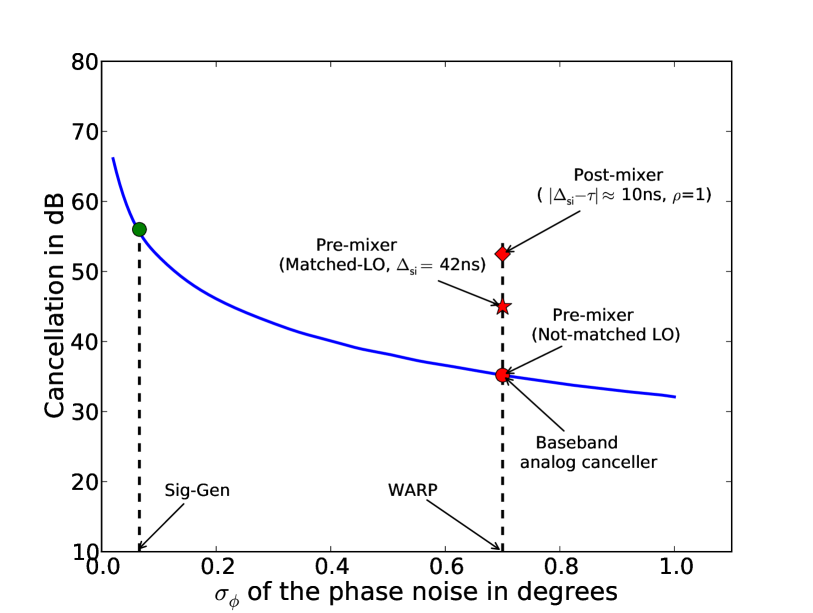
Figure 7: Amount of active analog cancellation possible in different types of cancellers as function of phase noise. The solid curve is a plot of amount of cancellation possible in pre-mixer cancellers if LOs are not matched, as a function of the variance of phase noise.

Note that the strength of the self-interference before active analog cancellation is $|h_{\sf si}|^{2}$. Therefore (28) implies that the strength of residual self-interference after active analog cancellation is dependent on the strength of the self-interference before cancellation. The amount of active cancellation is given by $\frac{|h_{\sf si}|^{2}}{2|h_{\sf si}|^{2}\sigma_{\sf si}^{2}+\sigma_{\sf noise}^{2}}\leq\frac{1}{2\sigma_{\sf si}^{2}}$. Thus, $\frac{1}{2\sigma_{\sf si}^{2}}$ is an upper bound for the amount of cancellation in pre-mixer cancellers where the local oscillators in self-interference path and cancelling path are independent, which we plot in Figure 7. Since [5] is a pre-mixer canceller and is designed on WARP platform, where local oscillators in the cancelling and self-interference path are not matched, Figure 7 predicts the amount of active analog cancellation to be 35 dB which is very close to the amount of cancellation reported by [5].

Observation 2: If the local oscillators in the self-interference path and the cancelling path are matched, $\phi_{\sf si}(t)=\phi_{\sf cancel}(t)$, then we have

$$\mathbb{E}(|y_{\sf residue-analog}(t)|^{2})\approx 2|h_{\sf si}|^{2}\sigma_{\sf si}^{2}(1-R_{\phi_{\sf si}}(\Delta_{\sf si}))+\sigma_{\sf noise}^{2}.$$ (29)

Equation (29) indicates that for a small delay $\Delta_{\sf si}$, the measure of the time of flight of the self-interference signal, the temporal correlation of phase noise aids in reducing the residual self-interference in pre-mixer cancellers. In Section IV-D, we measured and plotted in Figure 6, the amount of active analog cancellation as a function of the delay $\Delta_{\sf si}$, for a narrowband signal source. For $\Delta_{\sf si}\approx 42$ns, the time of flight of self-interference signal for 12 meters, the measurements in Figure 6 tell us that matching local oscillators in the self-interference and cancelling path will yield an active analog cancellation of 45 dB. Thus, matching local oscillators, when WARP is used as a signal source, results in 10 dB higher active analog cancellation compared to when local oscillators are not matched. In [5], ergodic rate of full-duplex beats half-duplex only upto 3.5 meters (indoor). However, in [10], an additional 10 dB passive suppression results in higher ergodic rates for half-duplex upto 6 meters. Matching local oscillators in [10] will give another 10 dB increase in overall reduction making full-duplex attractive at reasonable WiFi ranges.

From (28) and (29), we know that the phase noise dependent residual scales linearly in strength with self-interference. Therefore at higher received self-interference powers, phase noise becomes the dominant source of residual self-interference after active analog cancellation in pre-mixer cancellers.

V-B Performance of different active analog cancellers with imperfect channel estimates

Now we analyze and compare the impact of phase noise on active analog cancellation in pre-mixer, post-mixer and baseband analog cancellers. In order to draw the comparison, we analyse the amount of active analog cancellation when the estimate of self-interference channel is imperfect for which we show the following:

Result 2: For pre-mixer, post-mixer, as well as baseband analog canceller, the amount of active cancellation is inversely proportional to the variance of phase noise. However, the constant of proportionality is different for each canceller leading to different amounts of active analog cancellation.

To model imperfection, we let $\widehat{\mathbf{h}}_{\sf si}(t)=\rho h_{\sf si}\delta(t-\tau)$ denote the imperfect channel estimate of the self-interference channel, where $(1-\rho)$ and $(\tau-\Delta_{\sf si})$ represent the error in estimate of channel attenuation and delay respectively. Setting $\rho=1$ and $\tau=\Delta_{\sf si}$, we obtain the special case of perfect channel estimates.

The objective of each of the cancellers is to create a perfect null for the self-interference signal. However, in presence of phase noise each canceller adds a slightly different cancelling signal to the self-interference signal. Based on the imperfect channel estimate, the canceller generates $-\rho h_{\sf si}x_{\sf si}(t-\tau)e^{-j\omega_{c}\tau}$ as the cancelling signal. The cancelling signal after downconversion at the receiver will appear in analog baseband as

$$x_{\sf cancel,pre}(t)=-\rho h_{\sf si}e^{j(-\omega_{c}\tau+\phi_{\sf cancel}(t)-\phi_{\sf down}(t))}h_{\sf si}x_{\sf si}(t-\tau).$$ (30)

Note that the cancelling signal in pre-mixer analog cancellers is actually added to the received signal at RF, and then the combined signal is downconverted. However, in (30) we explicitly show the contribution of the cancelling signal in the residual self-interference signal after downconversion.

For the post-mixer analog canceller, the equivalent of (30) can be written as

$$x_{\sf cancel,post}(t)=-\rho e^{j(-\omega_{c}\tau+\phi_{\sf cancel}(t-\tau)-\phi_{\sf down}(t))}h_{\sf si}x_{\sf si}(t-\tau).$$ (31)

Note that (30) and (31) differ in the amount of delay the transmitter phase noise encounters. We remind the reader that in post-mixer analog cancellers, the cancelling signal is identical to the transmitted signal until after upconversion and therefore the phase noise $\phi_{\sf cancel}(t)=\phi_{\sf si}(t)$.

Finally, in baseband analog cancellers the cancelling signal has the following contribution to the residual self-interference

$$x_{\sf cancel,bb}(t)=-\rho e^{-j\omega_{c}\tau}h_{\sf si}x_{\sf si}(t-\tau).$$ (32)

The cancelling signal in (32) is not perturbed by any phase noise because the cancelling signal does not go through the RF chain itself.

Having described the cancelling signal, we can now write the residual self-interference for pre-mixer, post-mixer and baseband analog cancellers by adding the cancelling signal to the self-interference signal at the receiver. The residual self-interference for pre-mixer cancellers is

$$y_{\sf residual-analog}(t)=e^{-j(\omega_{c}\Delta_{\sf si}+\phi_{\sf si}(t-\Delta_{\sf si})-\phi_{\sf down}(t))}h_{\sf si}x_{\sf si}(t-\Delta_{\sf si})+x_{\sf cancel,pre}(t)+z_{\sf noise}(t).$$ (33)

The residual self-interference for post-mixer and baseband analog cancellers is defined similar to (33), by substituting the appropriate cancelling signal from (31) and (32).

We are interested in the strength of the residual self-interference after analog cancellation, and a close approximation can be found making use of the assumption that $\phi_{\sf si}(t)<<1,\phi_{\sf cancel}(t)<<1,\phi_{\sf down}(t)<<1$. The computation is shown in the Appendix X-D and the resulting strength of the residual self-interference is listed in Table I. From Table I, we make the following important observations.

Observation 3: Due to imperfect channel estimates, the strength of the residual self-interference in all the cancellers is composed of two types of residuals. The first type of residual self-interference is dependent only on the self-interference signal and the second type is dependent on phase noise. For all cancellers, the first type of residual self-interference dependent only on the self-interference signal is $|h_{\sf si}|^{2}(1+|\rho|^{2}-2|\rho|R_{x_{\sf si}}(\Delta_{\sf si}-\tau))$ which vanishes if $\rho=1$ and $\tau=\Delta_{\sf si}$, i.e., when perfect channel estimate is available. The second type of residual self-interference, dependent upon phase noise, scales with the variance of phase noise, as well as the strength of the self-interference channel $|h_{\sf si}|^{2}$, for all the cancellers. Due to the second type of residual self-interference linearly scaling with the variance of phase noise, the amount of active analog cancellation in the pre-mixer, post-mixer and baseband analog cancellers depend on the inverse of the variance of phase noise.

Observation 4: In post-mixer cancellers, the strength of residual self-interference due to phase noise is scaled by $(1-R_{\phi_{\sf si}}(\Delta_{\sf si}-\tau))$. The autocorrelation function $R_{\phi_{\sf si}}(.)$ approaches unity as the error in estimating the delay of the channel, $(\Delta_{\sf si}-\tau)$, is reduced, thereby reducing the residual self-interference. Unlike pre-mixer cancellers, where the delay $\Delta_{\sf si}$ determines the amount of residual self-interference, post-mixer cancellers can reduce residual self-interference by reducing the error in estimate of self-interference channel. Figure 7 shows the representative amount of cancellation of a post-mixer canceller for a narrowband signal source where $|\Delta_{\sf si}-\tau|\approx 10$ns and $\rho=1$. In principle, higher cancellation in post-mixer cancellers, as observed in [6, 8] is possible, because unlike pre-mixer cancellers, the residual self-interference continues to decrease as the error in the estimate of self-interference channel improves. In [3] USRP radios are used, whose phase noise variance (although not reported) is likely to be higher than WARP radios, thus explaining low, 20 dB, active analog cancellation.

Observation 5: In baseband analog cancellers, the residual self-interference scales as the sum of the variance of phase noise at the transmitter and the receiver. Due the asummption that phase noise in the local oscillator in the upconverting and downconverting circuit are independent, baseband analog cancellers have a phase noise dependent residual self-interference which does not depend on the delay $\Delta_{\sf si}$. Even when $\rho=1,\Delta_{\sf si}=\tau$, amount of cancellation is upper bounded by $\frac{1}{\sigma_{\sf si}^{2}+\sigma_{\sf down}^{2}}$, which is similar to the performance of pre-mixer cancellers with independent mixers in cancelling and self-interference path as shown in Figure 7.

VI Answer 2. Benefit of Digital Cancellation after Active Analog Cancellation

In this section, we answer “How do the amounts of cancellations by active analog and digital cancelers depend on each other in a cascaded system?”

VI-A Digital cancellation when active analog cancellation uses perfect channel estimate

Result 3: If active analog cancellation is performed with perfect channel estimates, then

• Digital cancellation does not reduce the strength of the residual self-interference at all, if $\phi_{\sf si}(t)$ and $\phi_{\sf cancel}(t)$ are identically distributed in pre- and post-mixer cancellers, and $\phi_{\sf si}(t)$ and $\phi_{\sf down}(t)$ are identically distributed in baseband analog cancellers.

• If $\phi_{\sf si}(t)$ and $\phi_{\sf cancel}(t)$ are not identically distributed, then under the assumption that $\phi_{\sf si}(t)<<1$, $\phi_{\sf cancel}(t)<<1$, $\phi_{\sf down}(t)<<1$, digital cancellation does not help.

For pre-mixer cancellers, the above result was already shown in our related work [1]. Digital cancellation can reduce the residual only if $y_{\sf resdiue-analog}[iT]$ is correlated with the self-interference signal $x_{\sf si}[iT]$. When $y_{\sf resdiue-analog}[iT]$ is correlated with $x_{\sf si}[iT]$, then digital cancellation can reduce the strength of the residual self-interference by subtracting a function of $x_{\sf si}[iT]$ from $y_{\sf residue-analog}[iT]$. We consider the residual after active analog cancellation in a pre-mixer canceller, as an example to show that $y_{\sf resdiue-analog}[iT]$ is not correlated with $x_{\sf si}[iT]$. The correlation of the residual signal with $x_{\sf si}[iT]$ yields

$$\mathbb{E}(y_{\sf residue-analog}[iT]x_{\sf si}[iT])$$ (34)

$$= \mathbb{E}(y_{\sf residual-si}[iT]x_{\sf si}[iT])+\mathbb{E}(z_{\sf noise}[iT]x_{\sf si}[iT])$$

$$\stackrel{{\scriptstyle\text{(a)}}}{{=}} \mathbb{E}\left(y_{\sf residual-si}[iT]x_{\sf si}[iT]\right)$$

$$\stackrel{{\scriptstyle\text{(b)}}}{{=}} h_{\sf si}\mathbb{E}\left(x_{\sf si}[iT]x_{\sf si}[iT-\Delta_{\sf si}](e^{j\phi_{\sf si}[iT]}-e^{j\phi_{\sf cancel}[iT-\Delta_{\sf si}]})e^{-j\phi_{\sf down}[iT]}\right)e^{-j\omega_{c}\Delta_{\sf si}}$$

$$\stackrel{{\scriptstyle\text{(c)}}}{{=}} h_{\sf si}R_{x_{\sf si}}(\Delta_{\sf si})\mathbb{E}\left(e^{j\phi_{\sf si}[iT]}-e^{j\phi_{\sf cancel}[iT-\Delta_{\sf si}]}\right)\mathbb{E}\left(e^{-j\phi_{\sf down}[iT]}\right)$$

where $y_{\sf residual-si}[iT]$ denotes the residual self-interference, in a pre-mixer canceller, minus thermal noise. In equation (34), equality (a) is true because the thermal noise is zero mean and independent of the self-interference, (b) is due to (25), (c) holds because phase noise is independent of the self-interference signal. Suppose that $\phi_{\sf si}(t)$ and $\phi_{\sf cancel}(t)$ are identically distributed, then $\mathbb{E}\left(e^{j\phi_{\sf si}[iT]}-e^{j\phi_{\sf cancel}[iT-\Delta_{\sf si}]}\right)=0$ letting us extend (34) to

$$\mathbb{E}(y_{\sf residue-analog}[iT]x_{\sf si}[iT])=0.$$ (35)

Under the approximation $\phi_{\sf si}(t)<<1$, $\phi_{\sf cancel}(t)<<1$, the residual self-interference signal in pre-radio cancellers is given by (26). From (26), we know that the residual self-interference has a component where the signal, $x_{\sf si}(t-\Delta_{\sf si})$, is multiplied by $j(\phi_{\sf si}(t-\Delta_{\sf si})-\phi_{\sf si}(t))$. The difference of phase noises, $j(\phi_{\sf si}(t-\Delta_{\sf si})-\phi_{\sf si}(t))$, is zero mean, independent of the signal, $x_{\sf si}(t-\Delta_{\sf si})$, and changes every sample. Thus, the residual self-interference in (26) can be considered as the sum of a fast-fading signal and thermal noise, where the fade is given by $j(\phi_{\sf si}(t-\Delta_{\sf si})-\phi_{\sf si}(t))$. Since the fade, $j(\phi_{\sf si}(t-\Delta_{\sf si})-\phi_{\sf si}(t))$, is zero mean and changes every sample, it cannot be estimated and thus digital cancellation cannot reduce the residual self-interference any further. More precisely,

$$\mathbb{E}(y_{\sf residue-analog}[iT]x_{\sf si}[iT])\approx h_{\sf si}R_{x_{\sf si}}(\Delta_{\sf si})\mathbb{E}\left(j\phi_{\sf si}[iT]-j\phi_{\sf cancel}[iT-\Delta_{\sf si}]\right)\mathbb{E}\left(e^{-j\phi_{\sf down}[iT]}\right)\stackrel{{\scriptstyle\text{(a)}}}{{=}}0$$ (36)

where (a) is true because phase noise is assumed to be zero mean. From (36), it is clear that the residual self-interference after active analog cancellation is uncorrelated to the self-interference signal and thus digital cancellation does not cancel self-interference any further.

The result that the residual self-interference after active analog cancellation not correlated to $x_{\sf si}[iT]$ when perfect channel estimates are available is not limited to pre-mixer cancellers. In post-mixer cancellers, perfect estimates for active analog cancellation imply that the residual is only thermal noise, which is naturally uncorrelated to the self-interference. In baseband cancellers, the correlation of the residual and self-interference signal can be written as

$$\mathbb{E}(y_{\sf residue-analog}[iT]x_{\sf si}[iT])$$

$$= h_{\sf si}\mathbb{E}\left(x_{\sf si}[iT]x_{\sf si}[iT-\Delta_{\sf si}](e^{j\phi_{\sf si}[iT]}-e^{j\phi_{\sf down}[iT-\Delta_{\sf si}]})\right)e^{-j\omega_{c}\Delta_{\sf si}}+\mathbb{E}(x_{\sf si}[iT]z_{\sf noise}[iT])\stackrel{{\scriptstyle\text{(a)}}}{{=}}0,$$

where (a) holds when $\phi_{\sf si}(t)$ and $\phi_{\sf down}(t)$ are identically distributed. If $\phi_{\sf si}(t)$ and $\phi_{\sf down}(t)$ are not distributed identically, then correlation of the self-interference signal with the residual self-interference is approximately zero if $\phi_{\sf si}[iT]<<1,\phi_{\sf down}[iT]<<1$. Digital cancellation is form of active cancellation, much like active analog cancellation. When perfect channel estimates are available, successively performing active cancellation is equivalent to actively cancelling in analog domain once.

VI-B Digital cancellation when active analog cancellation uses imperfect channel estimate

Result 4: If active analog cancellation uses imperfect channel estimates, then digital cancellation following it can cancel the residual correlated with the self-interference signal, thereby reducing its strength. However, the sum of the cascaded stages of active cancellation is limited by the phase noise properties and the error in channel estimate used for active analog cancellation

VI-B1 Pre-mixer canceller

As an example, let us consider the residual self-interference in pre-mixer canceller. Let us define the residual self-interference channel as

$$\mathbf{h}_{\sf residual-si}[iT]=h_{\sf si}(\delta[iT-\Delta_{\sf si}]e^{-j\omega_{c}\Delta_{\sf si}}-\rho\delta[iT-\tau]e^{-j\omega_{c}\tau}).$$ (37)

Then, the residual self-interference signal in the digital domain can be written as

$$\mathbf{h}_{\sf residual-si}[iT]\ast x_{\sf si}[iT]e^{j(\phi_{\sf cancel}[iT]-\phi_{\sf down}[iT])}+r_{\sf phase-noise,pre}[iT]+z_{\sf noise}[iT],$$ (38)

where

$$r_{\sf phase-noise,pre}[iT]=jh_{\sf si}e^{-j\omega_{c}\Delta_{\sf si}}x_{\sf si}[iT-\Delta_{\sf si}](\phi_{\sf si}[iT-\Delta_{\sf si}]-\phi_{\sf cancel}[iT])e^{j(\phi_{\sf cancel}[iT]-\phi_{\sf down}[iT])}$$ (39)

is the residual which is dependent on phase noise and uncorrelated with the self-interference signal $x_{\sf si}[iT]$. The digital canceller can use an estimate of the residual self-interference channel, $\widehat{\mathbf{h}}_{\sf residual-si}[iT]$, to generate a cancelling signal,$-\widehat{\mathbf{h}}_{\sf residual-si}[iT]\ast x_{\sf si}[iT]$, which will result in a residual self-interference given by

$$y_{\sf residue-digital}[iT] = (\mathbf{h}_{\sf residual-si}[iT])\ast x_{\sf si}[iT])e^{j(\phi_{\sf cancel}[iT]-\phi_{\sf down}[iT])}-\widehat{\mathbf{h}}_{\sf residual-si}[iT]\ast x_{\sf si}[iT]$$ (40)

$$+r_{\sf phase-noise,pre}[iT]+z_{\sf noise}[iT]$$

$$\approx (\mathbf{h}_{\sf residual-si}[iT]-\widehat{\mathbf{h}}_{\sf residual-si}[iT])\ast x_{\sf si}[iT]+r_{\sf phase-noise,pre}[iT]$$

$$+j\mathbf{h}_{\sf residual-si}[iT]\ast x_{\sf si}[iT](\phi_{\sf cancel}[iT]-\phi_{\sf down}[iT])+z_{\sf noise}[iT].$$

The strength of the residual self-interference after digital cancellation is

$$\mathbb{E}(|y_{\sf residue-digital}[iT]|^{2})$$ (41)

$$\approx \mathbb{E}(|(\mathbf{h}_{\sf residual-si}[iT]-\widehat{\mathbf{h}}_{\sf residual-si}[iT])\ast x_{\sf si}[iT]|^{2})+\mathbb{E}(|r_{\sf phase-noise}[iT]|^{2})$$

$$+ \mathbb{E}(|(\mathbf{h}_{\sf residual-si}[iT]\ast x_{\sf si}[iT])(\phi_{\sf cancel}[iT]-\phi_{\sf down}[iT])|^{2})+\mathbb{E}(|z_{\sf noise}[iT]|^{2})$$

$$= \underbrace{\mathbb{E}(|(\mathbf{h}_{\sf residual-si}[iT]-\widehat{\mathbf{h}}_{\sf residual-si}[iT])\ast x_{\sf si}[iT]|^{2})}_{\text{imperfect estimate in digital domain}}+\underbrace{2|h_{\sf si}|^{2}\sigma_{\sf si}^{2}(1-R_{\phi_{\sf si}}(\Delta_{\sf si}))}_{\text{phase noise}}+\sigma_{\sf noise}^{2}$$

$$+\underbrace{\mathbb{E}(|(\mathbf{h}_{\sf residual-si}[iT]\ast x_{\sf si}[iT])|^{2})}_{\text{imperfect estimate in analog domain}}(\sigma_{\sf si}^{2}+\sigma_{\sf down}^{2}).$$

We make the following two observations from (41).

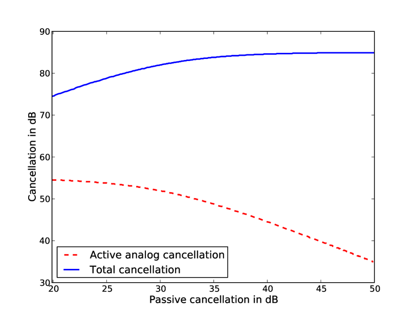
Figure 9: Total cancellation represents the sum of passive and active analog cancellation when operated in cascade in a pre-mixer canceller.

Observation 6: The amount of residual self-interference after digital cancellation stage is lower bounded by $2|h_{\sf si}|^{2}\sigma_{\sf si}^{2}(1-R_{\sf si}(\Delta_{\sf si}))+\sigma_{\sf noise}^{2}$, which, we recall from Section V-A, is the strength of residual self-interference after active analog cancellation that uses perfect estimate of self-interference channel. If the digital canceller uses perfect estimate of the residual self-interference channel, $\widehat{\mathbf{h}}_{\sf residual-si}[iT]=\mathbf{h}_{\sf residual-si}[iT]$, then it can eliminate the residual that depends only on self-interference signal entirely. Figure 9 shows the amount of digital cancellation possible as a function of active analog cancellation for a pre-mixer canceller where the local oscillators in the cancelling and self-interference path are independent which implies that $R_{\phi_{\sf si}}(\Delta_{\sf si})=0$. Figure 9 explains the trend of active analog vs. digital cancellation reported in [10], that the sum total active cancellation of active analog and digital stages is no more than 35 dB, which is the amount of cancellation achieved when the analog stage uses perfect estimates.

Observation 7: If $\sigma_{\sf down}^{2}>>\sigma_{\sf si}^{2}$, then the receiver phase noise will be a dominant source of bottleneck in digital cancellation. In computing the contribution of receiver phase noise to residual self-interference signal, we note that the variance of receiver phase noise is scaled by strength of the residual self-interference channel. Poor active analog cancellation implies that $\mathbb{E}(|(\mathbf{h}_{\sf residual-si}[iT]\ast x_{\sf si}[iT]|^{2})$ is large. Therefore, as depicted in Figure 9, poor active analog cancellation results in less overall cancellation, even when digital cancellation uses perfect estimate of self-interference channel.

VI-B2 Post-mixer cancellers

In post-mixer cancellers too, the digital cancellation when cascaded with active analog cancellation can only cancel the portion of residual self-interference that is correlated with the self-interference signal itself.

For post-mixer cancellers, the residual self-interference channel is defined as in (37) and the phase noise dependent residual self-interference is given by

$$r_{\sf phase-noise,post}=jh_{\sf si}e^{-j\omega_{c}\Delta_{\sf si}}x_{\sf si}[iT-\Delta_{\sf si}](\phi_{\sf si}[iT-\Delta_{\sf si}]-\phi_{\sf si}[iT-\tau])e^{j(\phi_{\sf si}[iT-\tau]-\phi_{\sf down}[iT])}.$$ (42)

The residual self-interference before digital cancellation will be

$$\mathbf{h}_{\sf residual-si}[iT]\ast x_{\sf si}[iT]e^{j(\phi_{\sf si}[iT-\tau]-\phi_{\sf down}[iT])}+r_{\sf phase-noise,post}[iT]+z_{\sf noise}[iT].$$ (43)

Note that the form of (43) is very similar to (38) and thus, without repeating the steps, we can write the residual in post-mixer cancellers after digital cancellation with imperfect estimates as

$$\mathbb{E}(|y_{\sf residual-digital}[iT]|^{2})$$ (44)

$$= \mathbb{E}(|(\mathbf{h}_{\sf residual-si}[iT]-\widehat{\mathbf{h}}_{\sf residual-si}[iT])\ast x_{\sf si}[iT]|^{2})+2|h_{\sf si}|^{2}\sigma_{\sf si}^{2}(1-R_{\phi_{\sf si}}(\Delta_{\sf si}-\tau))+\sigma_{\sf noise}^{2}$$

$$+\mathbb{E}(|(\mathbf{h}_{\sf residual-si}[iT]\ast x_{\sf si}[iT])|^{2})(\sigma_{\sf si}^{2}+\sigma_{\sf down}^{2})$$

Note that (44) is lower bounded by $2|h_{\sf si}|^{2}\sigma_{\sf si}^{2}(1-R_{\phi_{\sf si}}(\Delta_{\sf si}-\tau))+\sigma_{\sf noise}^{2}$, which itself is the lower bound on the strength of the residual when active analog cancellation uses imperfect estimate of the channel. Thus, even in post-mixer cancellers, more digital cancellation is possible when active analog cancellation cancels less. However, the sum of cancellation is no more than $1/(2\sigma_{\sf si}^{2}(1-R_{\phi_{\sf si}}(\Delta_{\sf si}-\tau))$, an expression which is solely dependent on phase noise.

VI-B3 Baseband analog cancellers

For baseband analog cancellers, let the residual self-interference channel be defined as in (37), and the residual dependent on phase noise be given by

$$r_{\sf phase-noise,bb}[iT]=jh_{\sf si}e^{-j\omega_{c}\Delta_{\sf si}}x_{\sf si}[iT-\Delta_{\sf si}](\phi_{\sf si}[iT-\Delta_{\sf si}]-\phi_{\sf down}[iT]).$$ (45)

The residual self-interference before digital cancellation be written as

$$\mathbf{h}_{\sf residual-si}[iT]\ast x_{\sf si}[iT]+r_{\sf phase-noise,bb}[iT]+z_{\sf noise}[iT].$$ (46)

Using $\widehat{\mathbf{h}}_{\sf residual-si}[iT]\ast x_{\sf si}[iT]$ as the cancelling signal, the strength of residual after imperfect digital cancellation is given by

$$\mathbb{E}(|y_{\sf residue-digital}[iT]|^{2})$$ (47)

$$= \mathbb{E}(|(\mathbf{h}_{\sf residual-si}[iT]-\widehat{\mathbf{h}}_{\sf residual-si}[iT])\ast x_{\sf si}[iT]|^{2})+\mathbb{E}(|r_{\sf phase-noise,bb}[iT]|^{2})+\mathbb{E}(|z_{\sf noise}[iT]|^{2})$$

$$= \mathbb{E}(|(\mathbf{h}_{\sf residual-si}[iT]-\widehat{\mathbf{h}}_{\sf residual-si}[iT])\ast x_{\sf si}[iT]|^{2})+|h_{\sf si}|^{2}(\sigma_{\sf si}^{2}+\sigma_{\sf down}^{2})+\sigma_{\sf noise}^{2}$$

$$\geq |h_{\sf si}|^{2}(\sigma_{\sf si}^{2}+\sigma_{\sf down}^{2})+\sigma_{\sf noise}^{2}.$$

The lower bound in (47) is the strength of residual self-interference after active analog cancellation is performed with perfect channel estimates in baseband cancellers. The lower bound in (47) is achievable if the digital canceller has perfect estimate of the residual self-interference channel. Thus, serially concatenated active analog cancellation and digital cancellation are interdependent in such way that their sum is bounded by $\frac{1}{\sigma_{\sf si}^{2}+\sigma_{\sf down}^{2}}$. One distinction in baseband analog cancellers is that unlike pre-mixer or post-mixer cancellers, the residual does not depend explicitly on the quality of active analog cancellation, i.e., $\mathbf{h}_{\sf residual-si}[iT]$, rather is dependent upon $(\mathbf{h}_{\sf residual-si}[iT]-\widehat{\mathbf{h}}_{\sf residual-si}[iT])$, the quality of digital cancellation only.

VII Answer 3. Influence of Passive Suppression on Active Cancellation

In this section, we answer “How and when does passive suppression impact the amount of analog cancellation?” We show that the amount of passive suppression can impact the amount of active analog cancellation in pre-mixer cancellers.

So far, we have considered a self-interference channel with only a single delay tap. Now, let us consider a self-interference channel with two non-zero taps, which can be considered as taps representing line of sight and the reflected components. Let the two-tap self-interference channel be $\mathbf{h}_{\sf si}(t)=h_{1}\delta(t-\Delta_{1})+h_{2}\delta(t-\Delta_{2})$, where $\Delta_{1}$ and $\Delta_{2}$ denote the delays of the line of sight and reflected component, therefore $\Delta_{1}<\Delta_{2}$. The average strength of the line of sight and reflected component are captured by $\mathbb{E}(|h_{1}|^{2})$ and $\mathbb{E}(|h_{2}|^{2})$. It is reasonable to assume that passive suppression can reduce the strength of the line of sight component. Therefore, the amount of passive suppression determines the ratio $\mathbb{E}(|h_{1}|^{2})/\mathbb{E}(|h_{2}|^{2})$.

Result 5: Higher passive suppression can result in lower active analog cancellation in pre-mixer cancellers. However, increasing passive suppression implies that sum of cascaded passive and active analog cancellation increases.

Assume self-interference channel is perfectly known. Then the cancelling signal in baseband is

$$x_{\sf cancel}(t)=-h_{1}x_{\sf si}(t-\Delta_{1})e^{-j\omega_{c}\Delta_{1}}-h_{2}x_{\sf si}(t-\Delta_{2})e^{-j\omega_{c}\Delta_{2}}.$$ (48)

In presence of phase noise, the residual self-interference is

$$y_{\sf residual}(t)$$

$$= h_{1}x_{\sf si}(t-\Delta_{1})e^{-j\omega_{c}\Delta_{1}}(e^{j\phi(t-\Delta_{1})}-e^{j\phi(t)})+h_{2}x_{\sf si}(t-\Delta_{2})e^{-j\omega_{c}\Delta_{2}}(e^{j\phi(t-\Delta_{2})}-e^{j\phi(t)})+z_{\sf noise}(t)$$

$$\approx jh_{1}x_{\sf si}(t-\Delta_{1})e^{-j\omega_{c}\Delta_{1}}(\phi(t-\Delta_{1})-\phi(t))+jh_{2}x_{\sf si}(t-\Delta_{2})e^{-j\omega_{c}\Delta_{2}}(\phi(t-\Delta_{2})-\phi(t))+z_{\sf noise}(t).$$

The strength of the residual signal is

$$\mathbb{E}(|y_{\sf residual}(t)|^{2}) \approx 2\mathbb{E}(|h_{1}|^{2})(1-R_{\phi_{\sf si}}(\Delta_{1}))+2\mathbb{E}(|h_{2}|^{2})(1-R_{\phi_{\sf si}}(\Delta_{2}))$$ (49)

$$+2\mathbb{E}\left(\text{Re}(h_{1}h_{2}^{\prime}x_{\sf si}(t-\Delta_{1})x^{\prime}_{\sf si}(t-\Delta_{2})e^{j\omega_{c}(\Delta_{2}-\Delta_{1})})\right)$$

$$(1+R_{\phi_{\sf si}}(\Delta_{1}-\Delta_{2})-R_{\phi_{\sf si}}(\Delta_{1})-R_{\phi_{\sf si}}(\Delta_{2}))\sigma_{\phi}^{2}.$$

The average residual self-interference can be estimated by assuming a distribution on the line of sight and the reflected component channel. From the experimental characterization of the self-interference channel in [22], we know that when the line of sight component is sufficiently suppressed, the self-interference channel is approximately a zero mean complex Gaussian random variable. Therefore, we have

$$\mathbb{E}(|y_{\mathsf{residual}}(t)|^{2})=\mathbb{E}(|h_{1}|^{2})(1-R_{\phi_{\mathsf{si}}}(\Delta_{1}))+\mathbb{E}(|h_{2}|^{2})(1-R_{\phi_{\mathsf{si}}}(\Delta_{2})),$$ (50)

assuming the independence of $h_{1}$ and $h_{2}$. If either $\mathbb{E}(|h_{1}|^{2})$ or $\mathbb{E}(|h_{2}|^{2})$ is reduced, it amounts to increasing the passive suppression. The design principle that increasing passive suppression reduces total residual self-interference is confirmed by equation (50) and it is also depicted in Figure 9.

The amount of active analog cancellation is obtained by computing the ratio of the strength of self-interference before and after active analog cancellation which is

$$\frac{\mathbb{E}(|h_{1}|^{2}+|h_{2}|^{2})}{\mathbb{E}(|h_{1}|^{2})(1-R_{\phi_{\sf si}}(\Delta_{1}))+\mathbb{E}(|h_{2}|^{2})(1-R_{\phi_{\sf si}}(\Delta_{2}))}.$$ (51)

The strength of the line of sight component, $\mathbb{E}(|h_{1}|^{2})$, varies as the coupling between transmit and receive antenna on the full-duplex node changes. At one extreme if passive suppression is low and line of sight is dominant, $\mathbb{E}(|h_{1}|^{2})/\mathbb{E}(|h_{2}|^{2})>>1$, then the amount of active analog cancellation possible is $1/(1-R_{\phi_{\sf si}}(\Delta_{1}))$. At the other extreme, if passive suppression is very high and the strength of line of sight component is negligible, then the amount of active analog cancellation possible is $1/(1-R_{\phi_{\sf si}}(\Delta_{2}))$. Thus, amount of passive suppression influences the amount of active analog cancellation. Moreover, since $\Delta_{1}<\Delta_{2}$ implies $1/(1-R_{\phi_{\sf si}}(\Delta_{1}))>1/(1-R_{\phi_{\sf si}}(\Delta_{2}))$, thus more passive suppression implies less active analog cancellation. In Figure 9 we plot the amount of active cancellation as a function of the strength of the line of sight component. Note that the total cancellation is maximized when passive suppression is maximum, however active analog cancellation reduces as passive suppression increases.

VIII Signal Model for Full-Duplex

Using the analyses in Sections V and VI, we develop a signal model for SISO full-duplex communication, and then extend it to the MIMO and wideband cases.

VIII-A Narrowband signal model

We present a digital baseband signal model which captures the effect of phase noise and imperfection in channel estimate by considering the residual self-interference after: (a) active analog cancellation and (b) digital cancellation cascaded with active analog cancellation. For both (a) and (b), the channel estimates are assumed to be imperfect.

Active analog cancellation with imperfect estimates

For pre-mixer cancellers the residual self-interference is given by (59). Since phase noise is assumed to be zero mean Gaussian, the linear combination of several phase noise terms is also Gaussian. Also, phase noise is assumed to be small, therefore $e^{j(\phi_{\sf si}(t-\Delta_{\sf si})-\phi_{\sf cancel}(t))}\approx 1$. Then the received signal at $\sf N$1, which is a combination of residual self-interference, signal of interest and thermal can be written as

$$y_{1}[iT] = \sqrt{P_{\sf signal}}\mathbf{h}_{\sf signal}[iT]\ast x_{\sf signal}[iT]+\sqrt{P_{\sf si}}|h_{\sf si}|\beta_{\phi}z_{\sf phase-noise}[iT]$$ (52)

$$+\sqrt{P_{\sf si}}\mathbf{h}_{\sf residual-si}[iT]\ast x_{\sf si}[iT]+z_{\sf noise}[iT],$$

where $z_{\sf phase-noise}[iT]$ is a zero mean AWGN with unit variance independent of the thermal noise and signal of interest. The signal $x_{\sf signal}[iT]$ is of unit variance and $P_{\sf si}$ and $P_{\sf signal}$ are power constraints at $\sf N$1 and $\sf N$2 respectively. The contribution of phase noise to the residual self-interference is captured by $\beta_{\phi}$ whose value is given in Table II.

For post-mixer cancellers, as well as baseband analog cancellers, the contribution of phase noise to the residual is different than pre-mixer cancellers. However, the form of the residual self-interference after active analog cancellation in post-mixer and baseband analog cancellers is given by (61) and (63) respectively, which is similar to (59). Therefore the signal model (52) holds for post-mixer and baseband analog cancellers too. The parameter $\beta_{\phi}$ for each canceller can be obtained from Table II.

Imperfect estimates in active analog and digital cancellation

After digital cancellation, the residual depends on the quality of the estimate of residual self-interference channel, in addition to phase noise. For pre-mixer cancellers, the residual is given by (40) and the strength of the residual is given by (41), which allows us to write the received signal at $\sf N$1 as

$$y_{1}[iT] = \sqrt{P_{\sf signal}}\mathbf{h}_{\sf signal}[iT]\ast x_{\sf signal}[iT]+\sqrt{P_{\sf si}}|h_{\sf si}|\gamma_{\phi}z_{\sf phase-noise}[iT]$$ (53)

$$+\sqrt{P_{\sf si}}(\mathbf{h}_{\sf residual-si}[iT]-\widehat{\mathbf{h}}_{\sf residual-si}[iT])\ast x_{\sf si}[iT])+z_{\sf noise}[iT],$$

where $\gamma_{\phi}$ is a parameter dependent on the phase noise and the quality of active analog cancellation. For post-mixer and baseband analog cancellers, the signal model in (53) is modified appropriately by changing the parameter $\gamma_{\phi}$, which is computed in (44) and (47) respectively, and populated in Table II.

VIII-B Wideband signal model

Wideband full-duplex is implemented in [7, 6]. In wideband full-duplex, the self-interference channel need not be frequency flat [22, 13]. To derive a signal model for wideband full-duplex, we treat it as a combination of several narrowband full-duplex systems. Let the overall bandwidth be $W$ and the coherence bandwidth of the self-interference channel be $w$, then wideband channel is composed of $K=\lceil\frac{W}{w}\rceil$ narrowband channels. Let the $k^{\text{th}}$ narrowband channel be denoted by $h_{{\sf si},k}\delta(t-\Delta_{{\sf si},k})$. If the bandwidth is much smaller than the carrier frequency, $W<<\omega_{c}$, then the phase jitter over the band of interest can be assumed to be independent of the bandwidth [12].

The signal model for wideband full-duplex can be described by explicitly writing the expression for received signal in each of $K$ narrowband channels. After active analog cancellation with imperfect channel estimate, the received signal in the $k^{\rm th}$ narrrowband channel is given by

$$y_{1,k}[iT] = \mathbf{h}_{\mathsf{signal},k}[iT]\ast x_{\mathsf{signal},k}[iT]+\sqrt{P_{\mathsf{si},k}}|h_{\mathsf{si},k}|\gamma_{\phi}z_{\mathsf{phase-noise},k}[iT]$$ (54)

$$+\mathbf{h}_{\mathsf{residual-si},k}[iT]\ast x_{\mathsf{si},k}[iT]+z_{\sf noise}[iT],$$

where $P_{\mathsf{si},k}$ is power constraint for each band. Note that, while the phase noise in each band scales according to the transmit power in that band, the thermal noise floor remains constant. To compare the bottleneck in narrowband vs. wideband let us assume the total power in both is the same, say $P$. As a simplifying assumption, let $|h_{\sf si,k}|=|h_{\sf si}|$. In the narrowband system, the strength of residual self-interference due to phase noise is $P|h_{\sf si}|^{2}\beta_{\phi}^{2}$, which is the same as the strength of the residual self-interference due to phase noise is in wideband, i.e., $\sum_{i=1}^{K}P_{\sf si,k}|h_{\sf si,k}|^{2}\beta_{\phi}^{2}=P|h_{\sf si}|^{2}\gamma_{\phi}^{2}$. On the other hand, if the thermal noise floor in narrowband is given by the variance $\sigma_{\sf noise}^{2}$, then the variance of the noise over wideband is $K\sigma_{\sf noise}^{2}$. The signal model after digital cancellation can be written by simply replacing $\beta_{\phi}$ by $\gamma_{\phi}$, and $\mathbf{h}_{\mathsf{residual-si},k}[iT]$ with $\widehat{\mathbf{h}}_{\mathsf{residual-si},k}[iT]$ in (54).

VIII-C MIMO full-duplex signal model

To extend the narrowband SISO model (52), we assume a MIMO system with $M$ transmit antenna and $N$ received antenna. The self-interference at each of the receivers is due to the sum of $M$ transmissions, one from each transmit antenna. If the transmit radio chain for each antenna has an independent local oscillator, then the residual self-interference due to phase noise is the sum of $M$ independent residuals due to phase noise in a SISO system. Then, the received signal at the $n^{\rm th}$ receiver of the full-duplex node $\sf N$1 is given as

$$y_{1,n}[iT] = \sum_{m=1}^{M}\sqrt{P_{\mathsf{signal},m}}\mathbf{h}_{\mathsf{signal},mn}[iT]\ast x_{\mathsf{signal},m}[iT]+\gamma_{\phi}\sqrt{\sum_{m=1}^{M}|h_{\mathsf{si},m}|^{2}P_{\mathsf{si},m}}z_{\mathsf{phase-noise},n}[iT]$$ (55)

$$+\sum_{i=1}^{M}\mathbf{h}_{\mathsf{residual-si},mn}[iT]\ast x_{\sf si,m}[iT]+z_{\mathsf{noise},n}[iT],$$

where $z_{\mathsf{phase-noise},n}[iT]$ is unit variance, while $z_{\mathsf{noise},n}[iT]$ has a variance of $\sigma_{\sf noise}^{2}$. The $\mathbf{h}_{\mathsf{signal},mn}[iT]$ represents the channel for the signal of interest from $m^{\rm th}$ transmitter to $n^{\rm th}$ receiver. The self-interference channel and the residual self-interference channel at $\sf N$1 is represented by $\mathbf{h}_{\mathsf{si},mn}[iT]$ and $\mathbf{h}_{\mathsf{residual-si},mn}[iT]$ respectively. Power constraints at the $m^{\rm th}$ transmitter for the signal of interest and self-interference is $P_{\mathsf{signal},m}$ and $P_{\mathsf{si},m}$ respectively. To qualitatively understand the MIMO model in (55), consider the special case where all the self-interference channels have identical magnitude, the residual self-interference is simply $M$ times the residual self-interference for SISO. To describe the signal model after digital cancellation, we can extend the signal model in (55) by following the steps used to extend (52) to (53).

IX Conclusion

In this paper, we provided an analytical explanation of experimentally observed performance bottlenecks in full-duplex systems. Our analysis clearly shows that phase noise is a major bottleneck today and thus reducing the phase noise figure of radio mixers could lead to improved self-interference cancellation.

X Appendix

X-A Lower bound for autocorrelation function

Let $S(f)$ be power spectral density of the bandlimited function $x(t)$ such that $S(f)=0$ outside $[-F/2,F/2]$. Due to the power constraint, we have $\int\limits_{-F/2}^{F/2}S(f)df=1$. To evaluate the autocorrelation function $R(.)$ at $\tau$

$$R(\tau) = \int\limits_{-\infty}^{\infty}S(f)e^{-j2\pi f\tau}df=\int\limits_{-F/2}^{F/2}S(f)e^{-j2\pi f\tau}df=2\int\limits_{0}^{F/2}S(f)\cos{(2\pi f\tau)}df$$ (56)

$$\stackrel{{\scriptstyle\text{(a)}}}{{\approx}} 2\int\limits_{0}^{F/2}S(f)(1-c_{1}f^{2}\tau^{2})df=1-c_{1}\tau^{2}\int\limits_{0}^{F/2}f^{2}S(f)df\geq 1-(c_{1}F^{2}/4)\tau^{2}\left(2\int\limits_{0}^{F/2}S(f)df\right)$$

$$= 1-c\tau^{2},$$

where (a) holds if $\tau$ is small, and $c=c_{1}F^{2}/4$.

X-B Estimating the suitable scaling for cancellation for delay $d$

Let us denote by $a_{1}=h_{1}e^{-j(\omega_{c}+\omega)\Delta_{1}}$ and $a_{2}=h_{2}e^{-j(\omega_{c}+\omega)\Delta_{2}}$. If (12) and (13) is true, then

$$h_{c}(d) = \frac{\sum_{i=1}^{N}y_{2}[(i-d)T]^{\prime}y_{1}[iT]}{\sum_{i=1}^{N}|y_{2}[(i-d)T]|^{2}}$$

$$= \frac{\sum_{i=1}^{N}(a_{2}^{\prime}x[(i-d)T]^{\prime}+z_{2}[(i-d)T]^{\prime})(a_{1}x[iT]+z_{1}[iT])}{\sum_{i=1}^{N}(a_{2}^{\prime}x[(i-d)T]^{\prime}+z_{2}[(i-d)T]^{\prime})(a_{2}x[(i-d)T]+z_{2}[(i-d)T])}$$

$$= \frac{\sum_{i=1}^{N}(a_{2}^{\prime}e^{j\omega dT}x[iT]^{\prime}+z_{2}[(i-d)T]^{\prime})(a_{1}x[iT]+z_{1}[iT])}{\sum_{i=1}^{N}(a_{2}^{\prime}x[(i-d)T]^{\prime}+z_{2}[(i-d)T]^{\prime})(a_{2}x[(i-d)T]+z_{2}[(i-d)T])}$$

$$= \frac{\sum_{i=1}^{N}(a_{2}^{\prime}a_{1}e^{j\omega dT}|x[iT]|^{2}+a_{1}x[iT]z_{2}[(i-d)T]^{\prime}+a_{2}e^{-j\omega dT}x[iT]^{\prime}z_{1}[iT]+z_{2}[(i-d)T]^{\prime}z_{1}[iT])}{\sum_{i=1}^{N}(|a_{2}|^{2}|x_{2}[iT]|^{2}+|z_{2}[iT]|^{2}+2\text{Re}\{a_{2}x_{2}[iT]z_{2}[iT]^{\prime}\})}$$

Letting $N\to\infty$ we can replace the summations with expectations. Due to independence of thermal noise and the signal, we have

$$h_{c} = \frac{a_{2}^{\prime}a_{1}e^{j\omega dT}}{|a_{2}|^{2}+\sigma_{\sf noise}^{2}}=\frac{a_{1}}{a_{2}}e^{j\omega dT}\left(\frac{1}{1+\frac{\sigma_{\sf noise}^{2}}{|a_{2}|^{2}}}\right)\approx\frac{h_{1}}{h_{2}}e^{j((\omega_{c}+\omega)(\Delta_{2}-\Delta_{1})+\omega dT)}\left(1-\frac{\sigma_{\sf noise}^{2}}{|h_{2}|^{2}}\right)$$ (58)

X-C Calculating variance of phase noise

We derive the jitter from the spectrum of the phase noise as follows. Let the carrier frequency be denoted by $f_{c}$ and let the spectrum of the phase noise be specified as $\mathcal{L}(f)$ dBc/Hz where f is the frequency offset from the carrier frequency. The phase jitter in radians is given by $\Delta\theta_{\sf RMS}=\sqrt{\int_{f_{1}}^{f_{2}}10^{\frac{\mathcal{L}(f)}{10}}df}$, where $f_{2}-f_{1}$ would be bandwidth of the signal ($f_{1}$ being the lower offset and $f_{2}$ being the higher offset). Jitter in time is given by $\Delta t_{\sf RMS}=\frac{\Delta\theta_{\sf RMS}}{2\pi f_{c}}$ and the corresponding jitter in phase can be calculated as $\Delta\theta_{\sf RMS}=\frac{2\pi f_{c}\Delta t_{\sf RMS}}{\pi}$. For WARP radio, MAXIM 2829 [19], operating at a carrier frequency of 2.4GHz results in a time jitter of 0.83 picoseconds which corresponds to $\sigma_{\phi}=0.717^{\circ}$, and for the signal generator [21], operating at 2.2 GHz the phase noise variance is computed to be $\sigma_{\phi}=0.066$.

X-D Residual computations after active analog cancellations

Pre-mixer canceller: The residual is given by (33), which can be written as

$$y_{\sf residue-analog}(t) = h_{\sf si}e^{j(\phi_{\sf cancel}(t)-\phi_{\sf down}(t))}\left(x_{\sf si}(t-\Delta_{\sf si})e^{-j\omega_{c}\Delta_{\sf si}}e^{j(\phi_{\sf si}(t-\Delta_{\sf si})-\phi_{\sf cancel}(t))}-\rho x_{\sf si}(t-\tau)e^{-j\omega_{c}\tau}\right)$$ (59)

$$+z_{\sf noise}(t)$$

$$\approx h_{\sf si}e^{j(\phi_{\sf cancel}(t)-\phi_{\sf down}(t))}\underbrace{(x_{\sf si}(t-\Delta_{\sf si})e^{-j\omega_{c}\Delta_{\sf si}}-\rho x_{\sf si}(t-\tau)e^{-j\omega_{c}\tau})}_{\text{imperfect estimate}}$$

$$+h_{\sf si}e^{j\phi_{\sf cancel}(t)}e^{-j\omega_{c}\Delta_{\sf si}}x_{\sf si}(t-\Delta_{\sf si})\underbrace{\left(\phi_{\sf si}(t-\Delta_{\sf si})-\phi_{\sf cancel}(t)\right)}_{\text{phase noise}}+z_{\sf noise}(t).$$

The strength of the residual is given by

$$\mathbb{E}(|y_{\sf residue-analog}(t)|^{2})$$ (60)

$$\approx |h_{\sf si}|^{2}(1+\rho^{2}-2R_{x_{\sf si}}(\Delta_{\sf si}-\tau)\text{Re}\{\rho e^{-j\omega_{c}(\Delta_{\sf si}-\tau)}\})+2\sigma_{\sf si}^{2}(1-R_{\phi_{\sf si}}(\Delta_{\sf si}))+\sigma_{\sf noise}^{2}$$

$$\geq |h_{\sf si}|^{2}(\underbrace{1+\rho^{2}-2|\rho|R_{x_{\sf si}}(\Delta_{\sf si}-\tau)}_{\text{imperfect estimate}}+\underbrace{2\sigma_{\sf si}^{2}(1-R_{\phi_{\sf si}}(\Delta_{\sf si}))}_{\text{phase noise}})+\sigma_{\sf noise}^{2}.$$

Post-mixer canceller: The residual self-interference is given by

$$y_{\mathsf{residue-analog}}(t) = h_{\sf si}(x_{\sf si}(t-\Delta_{\sf si})e^{-j\omega_{c}\Delta_{\sf si}}e^{j\phi_{\sf si}(t-\Delta_{\sf si})}-\rho x_{\sf si}(t-\tau)e^{-j\omega_{c}\tau}e^{j\phi_{\sf si}(t-\tau)})e^{-j\phi_{\sf down}(t)}$$

$$+z_{\sf noise}(t)$$

$$\approx h_{\sf si}e^{j(\phi_{\sf si}(t-\tau)-\phi_{\sf down}(t))}\underbrace{(x_{\sf si}(t-\Delta_{\sf si})e^{-j\omega_{c}\Delta_{\sf si}}-\rho x_{\sf si}(t-\tau)e^{-j\omega_{c}\tau})}_{\text{imperfect estimate}}$$ (61)

$$+h_{\sf si}e^{j\phi_{\sf si}(t-\tau)}e^{-j\omega_{c}\Delta_{\sf si}}x_{\sf si}(t-\Delta_{\sf si})\underbrace{\left(\phi_{\sf si}(t-\Delta_{\sf si})-\phi_{\sf si}(t-\tau)\right)}_{\text{phase noise}}+z_{\sf noise}(t).$$

and its strength is given by

$$\mathbb{E}(|y_{\sf residue-analog}(t)|^{2})\geq|h_{\sf si}|^{2}(\underbrace{1+\rho^{2}-2|\rho|R_{x_{\sf si}}(\Delta_{\sf si}-\tau)}_{\text{imperfect estimate}}+\underbrace{2\sigma_{\sf si}^{2}(1-R_{\phi_{\sf si}}(\Delta_{\sf si}-\tau))}_{\text{phase noise}})+\sigma_{\sf noise}^{2}.$$ (62)

Baseband analog canceller: In baseband analog canceller, the residual self-interference is given by

$$y_{\sf residue-analog}(t) = h_{\sf si}e^{-j\omega_{c}\Delta_{\sf si}}x_{\sf si}(t-\Delta_{\sf si})(e^{j(\phi_{\sf si}(t-\Delta_{\sf si})-\phi_{\sf down}(t))})-\rho h_{\sf si}e^{-j\omega_{c}\tau}x_{\sf si}(t-\tau)+z_{\sf noise}(t)$$ (63)

$$\approx h_{\sf si}(e^{-j\omega_{c}\Delta_{\sf si}}x_{\sf si}(t-\Delta_{\sf si})-\rho e^{-j\omega_{c}\tau}x_{\sf si}(t-\tau))$$

$$+h_{\sf si}e^{-j\omega_{c}\Delta_{\sf si}}x_{\sf si}(t-\Delta_{\sf si})(j(\phi_{\sf si}(t-\Delta_{\sf si})-\phi_{\sf down}(t)))+z_{\sf noise}(t).$$

and it’s strength is given by

$$\mathbb{E}(|y_{\sf residue-analog}(t)|^{2})=|h_{\sf si}|^{2}(\underbrace{1+\rho^{2}-2|\rho|R_{x_{\sf si}}(\tau-\Delta_{\sf si})}_{\text{imperfect estimate}}+\underbrace{\sigma_{\sf si}^{2}+\sigma_{\sf down}^{2}}_{\text{phase noise}})+\sigma_{\sf noise}^{2}.$$ (64)

\begin{picture}(4310.0,2251.0)(1115.0,-2615.0)\end{picture}

Figure 1: Classification of methods of reducing self-interference

Figure 2: Block diagram representation of all the self-interference reduction methods in concatenation.

(a) At-RF active analog canceller

(b) At-Baseband active analog canceller.

Figure 3: Two architectures of analog cancellers differentiated based on whether the cancellation occurs at RF or analog baseband. The functions $r_{\sf up}(.)$ and $r_{\sf down}(.)$ represent the process of upconversion to RF and downconversion from RF respectively.

Figure 4: Schematic representation of the experiment in Section IV to acquire copies of a signals using a vector signal analyzer. WARP and Vector Signal Generator were two different signal sources considered in the experiment.

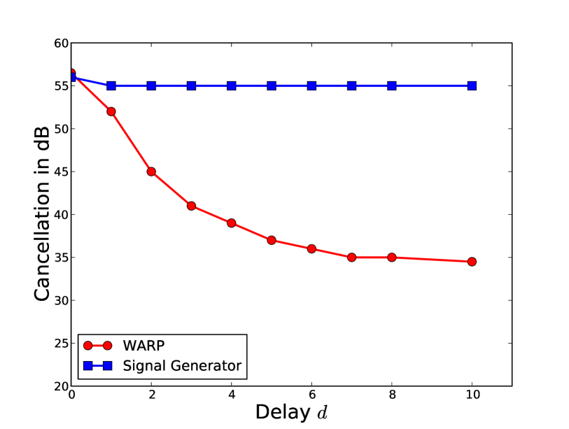
Figure 5: Amount of cancellation as a function of the delay for different signal sources measured from the experiment in Section IV. Also shown in our related work [1].

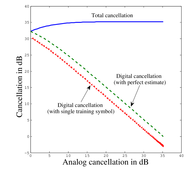
Figure 8: The relationship between amount of active analog cancellation and the amount of digital cancellation in a pre-mixer canceller is shown. Also, we assume $\sigma_{\sf si}^{2}=\sigma_{\sf down}^{2}$.

Type of canceller	Expected value of the strength of residual self-interference after active analog cancellation
Pre-mixer	$|h_{\sf si}|^{2}(1+|\rho|^{2}-2|\rho|R_{x_{\sf si}}(\Delta_{\sf si}-\tau)+2\sigma_{\sf si}^{2}(1-R_{\phi_{\sf si}}(\Delta_{\sf si}))+\sigma_{\sf noise}^{2}$
Post-mixer	$|h_{\sf si}|^{2}(1+|\rho|^{2}-2|\rho|R_{x_{\sf si}}(\Delta_{\sf si}-\tau)+2\sigma_{\sf si}^{2}(1-R_{\phi_{\sf si}}(\Delta_{\sf si}-\tau))+\sigma_{\sf noise}^{2}$
Baseband analog	$|h_{\sf si}|^{2}(1+|\rho|^{2}-2|\rho|R_{x_{\sf si}}(\Delta_{\sf si}-\tau)+(\sigma_{\sf si}^{2}+\sigma_{\sf down}^{2}))+\sigma_{\sf noise}^{2}$

TABLE I: Expected value of the strength of the residual self-interference after active analog cancellation with imperfect estimate of self-interference channel

	$\beta_{\phi}^{2}$ for active analog cancellation only	$\gamma_{\phi}^{2}$ for active analog + digital cancellation
	(imperfect estimate)	(both with imperfect estimates)
Pre-mixer	$2\sigma_{\sf si}^{2}(1-R_{\phi_{\sf si}}(\Delta_{\sf si}))$	$(1+|\rho|^{2}-2|\rho|R_{x_{\sf si}}(\tau-\Delta_{\sf si}))(\sigma_{\sf si}^{2}+\sigma_{\sf down}^{2})$
		$+2\sigma_{\sf si}^{2}(1-R_{\phi_{\sf si}}(\Delta_{\sf si}))$
Post-mixer	$2\sigma_{\sf si}^{2}(1-R_{\phi_{\sf si}}(\tau-\Delta_{\sf si}))$	$(1+|\rho|^{2}-2|\rho|R_{x_{\sf si}}(\tau-\Delta_{\sf si}))(\sigma_{\sf si}^{2}+\sigma_{\sf down}^{2})$
		$+2\sigma_{\sf si}^{2}(1-R_{\phi_{\sf si}}(\tau-\Delta_{\sf si}))$
Baseband canceller	$\sigma_{\sf si}^{2}+\sigma_{\sf down}^{2}$	$\sigma_{\sf si}^{2}+\sigma_{\sf down}^{2}$

TABLE II: Parameters defining the singal models in (52) and (53) for SISO narrowband, (54) for SISO wideband and (55) for MIMO full-duplex for different types of cancellers. We assume that $\sigma_{\sf si}=\sigma_{\sf cancel}$

References

- [1] A. Sahai, G. Patel, C. Dick, and A. Sabharwal, “Understanding the Impact of Phase Noise on Active Cancellation in Wireless Full-duplex,” in Proceedings of Asilomar Conference on Signals, Systems and Computers, 2012.
- [2] B. Radunovic, D. Gunawardena, P. Key, A. P. N. Singh, V. Balan, and G. Dejean, “Rethinking Indoor Wireless: Low Power, Low Frequency, Full Duplex,” Microsoft Research, Tech. Rep., 2009.
- [3] J. I. Choi, M. Jain, K. Srinivasan, P. Levis, and S. Katti, “Achieving Single Channel, Full Duplex Wireless Communications,” in Proceedings of ACM Mobicom, 2010.
- [4] A. Khandani, “Methods for spatial multiplexing of wireless two-way channels,” Oct. 19 2010, US Patent 7,817,641.
- [5] M. Duarte and A. Sabharwal, “Full-Duplex Wireless Communications Using Off-The-Shelf Radios: Feasibility and First Results,” in Proceedings of Asilomar Conference on Signals, Systems and Computers, 2010.
- [6] M. Jain, J. I. Choi, T. Kim, D. Bharadia, K. Srinivasan, S. Seth, P. Levis, S. Katti, and P. Sinha, “Practical, Real-time, Full Duplex Wireless,” in Proceeding of the ACM Mobicom, Sept. 2011.
- [7] A. Sahai, G. Patel, and A. Sabharwal, “Pushing the limits of full-duplex: Design and real-time implementation, http://arxiv.org/abs/1107.0607,” in Rice University Technical Report TREE1104, June 2011.
- [8] M. A. Khojastepour, K. Sundaresan, S. Rangarajan, X. Zhang, and S. Barghi, “The Case for Antenna Cancellation for Scalable Full-Duplex Wireless Communications,” in Proceedings of the 10th ACM Workshop on HotNets, 2011.
- [9] E. Aryafar, M. Khojastepour, K. Sundaresan, S. Rangarajan, and M. Chiang, “MIDU: enabling MIMO full duplex,” in Proceedings of ACM MobiCom, 2012.
- [10] M. Duarte, “Full-duplex Wireless: Design, Implementation and Characterization,” Ph.D. dissertation, Rice University, April.
- [11] M. Duarte, A. Sabharwal, V. Aggarwal, R. Jana, K. Ramakrishnan, C. Rice, and N. Shankaranarayanan, “Design and Characterization of a Full-duplex Multi-antenna System for WiFi Networks,” arXiv preprint arXiv:1210.1639, 2012.
- [12] P. Smith, “Little known characteristics of phase noise,” Application Note AN-741. Analog Devices, Inc.(August)., 2004.
- [13] E. Everett, M. Duarte, C. Dick, and A. Sabharwal, “Empowering Full-Duplex Wireless Communication by Exploiting Directional Diversity,” in Proceeding of Asilomar Conference on Signals, Systems and Computers. IEEE, 2011.
- [14] E. Everett, “Full-duplex Infrastructure Nodes: Achieving Long Range with Half-duplex Mobiles,” Master’s thesis, Rice University, 2012.
- [15] “QHX220,” http://www.intersil.com/content/dam/Intersil/documents/fn69/fn6986.pdf.
- [16] A. Quazi, “An overview on the time delay estimate in active and passive systems for target localization,” Acoustics, Speech and Signal Processing, IEEE Transactions on, vol. 29, no. 3, 1981.
- [17] P. E. D. Sheet, ““sma female power divider pe2014”.”
- [18] “Agilent VSA,” http://cp.literature.agilent.com/litweb/pdf/5989-1121EN.pdf.
- [19] “MAX2829 RF transceiver,” http://www.maxim-ic.com/datasheet/index.mvp/id/4532.
- [20] “Rice University WARP project,” http://warp.rice.edu.
- [21] “E4438C ESG Vector Signal Generator,” http://cp.literature.agilent.com/litweb/pdf/5988-4039EN.pdf.
- [22] M. Duarte, C. Dick, and A. Sabharwal, “Experiment Driven Characterization of Full-Duplex Wireless Communications,” in IEEE Transactions on Wireless Communications, To appear.