Shot noise of spin current and spin transfer torque

Abstract

We report the theoretical investigation of noise spectrum of spin current ($S^{\sigma}$) and spin transfer torque ($S^{\tau}$) for non-colinear spin polarized transport in a spin-valve device which consists of normal scattering region connected by two ferromagnetic electrodes (MNM system). Our theory was developed using non-equilibrium Green’s function method and general non-linear $S^{\sigma}-V$ and $S^{\tau}-V$ relations were derived as a function of angle $\theta$ between magnetization of two leads. We have applied our theory to a quantum dot system with a resonant level coupled with two ferromagnetic electrodes. It was found that for the MNM system, the auto-correlation of spin current is enough to characterize the fluctuation of spin current. For a system with three ferromagnetic layers, however, both auto-correlation and cross-correlation of spin current are needed to characterize the noise spectrum of spin current. Furthermore, the spin transfer torque and the torque noise were studied for the MNM system. For a quantum dot with a resonant level, the derivative of spin torque with respect to bias voltage is proportional to $\sin\theta$ when the system is far away from the resonance. When the system is near the resonance, the spin transfer torque becomes non-sinusoidal function of $\theta$. The derivative of noise spectrum of spin transfer torque with respect to the bias voltage $N_{\tau}$ behaves differently when the system is near or far away from the resonance. Specifically, the differential shot noise of spin transfer torque $N_{\tau}$ is a concave function of $\theta$ near the resonance while it becomes convex function of $\theta$ far away from resonance. For certain bias voltages, the period $N_{\tau}(\theta)$ becomes $\pi$ instead of $2\pi$. For small $\theta$, it was found that the differential shot noise of spin transfer torque is very sensitive to the bias voltage and the other system parameters.

1 Introduction

Electronic shot noise describes the fluctuation of current and is an intrinsic property of quantum devices due to the quantization of electron charge. In the past decade, the study of shot noise has attracted increasing attention[1] because it can give additional information that is not contained in the conductance or charge current. It can be used to probe the kinetics of electron[2] and investigate correlations of electronic wave functions[3]. In the study of shot noise $<(\Delta\hat{I})^{2}>$, the Fano Factor $F=<(\Delta\hat{I})^{2}>/2q<\hat{I}>$ is often used where $<\hat{I}>$ is the current. When $F>1$ it is referred as super-Poissonian noise, while $F<1$ corresponds to sub-Poissonian behavior. In general, for a quantum device, Pauli exclusion suppresses the shot noise and hence reduces the Fano factor[4, 5, 6] but Coulomb interaction can either suppress or enhance shot noise depending on system details[7, 8, 9, 10, 11]. The suppression of shot noise has been confirmed experimentally in quantum point contact[12, 13], single electron tunneling regime[14, 15], graphene nano-ribbon[16, 17], and atom-size metallic contacts[18, 19]. The enhancement of shot noise was also observed in GaAs based quantum contacts when the system is in the negative differential conductance region[20]. Recently, with the development of spintronics, polarized spin current especially pure spin current received much more attention. Less attention has been paid on the polarized spin current correlation compared with the charge current correlation[21, 22, 23, 24, 25, 26]. Shot noise of polarized spin current has been studied in several quantum devices including the MNM(ferromagnet-normal-ferromagnet)[27] and NMN(normal-magnetic-normal)[28]. In these devices, shot noise is expected to provide additional information about the spin-dependent scattering process and spin accumulation. It was shown that shot noise can be used to probe attractive or repulsive interactions in mesoscopic systems and to measure the spin relaxation time [29]. For a two-probe normal system (NNN system), it is well known that the charge current correlation between different probes (cross correlation noise) is negative definitely[30], but for a magnetic junction, the spin cross correlation noise between different probes is not necessarily negative due to spin flip mechanism. For example, Ref.[31] showed that the cross correlation can be positive at special Fermi energy due to Rashba interaction.

Recently, spin transfer torque (STT), predicted by Slonczewski[32, 33] and Berger[34], has been the subject of intensive investigations[35, 36, 37, 38]. Spin current can transfer spin angular momentum and be used to switch the magnetic orientation of ferromagnetic layers in GMR and TMR devices. Therefore, STT has potential applications[39] such as hard-disk read head[40], magnetic detection sensor[41], and random access memory (MRAM)[42], etc.. It comes from the absorption of the itinerant flow of angular momentum components normal to the magnetization direction and relies on the system spin polarized current. The noise spectrum of STT drastically affects the magneto-resistance behavior[43]. Many studies have focused on the spin transfer torque in various materials and under dc or ac condition. The correlation effect or quantum noise of spin transfer torque has not been studied so far. It is the purpose of this paper to fill this gap. In this paper, we have calculated the shot noise of particle current, spin current as well as spin transfer torque in the nonlinear regime for a magnetic quantum dot connected with two non-colinear magnetic electrodes. We found that for a MNM spin-valve system, the spin auto-correlation is enough to characterize the fluctuation of spin current. For a system with three ferromagnetic layers (MNMNM), however, both auto-correlation and cross-correlation are needed to characterize the fluctuation of spin current. For the quantum dot with a resonant level, the behavior of differential STT depends on whether the system on resonance or off resonance. When the system is off resonance, the differential STT reduces to the familiar result of tunneling barrier $(1/2)(I^{s}(\pi)-I^{s}(0))\sin\theta$ where $\theta$ is the angle between magnetic moments of ferromagnetic leads. If it is on resonance, the dependence of differential STT on $\theta$ becomes non-sinusoidal. The resonance also has influence on the noise spectrum of STT. If the system is near the resonance, noise spectrum of STT is a concave function of $\theta$ while it becomes a convex function far away from the resonance.

This paper is organized as follows. Firstly, we derive the general formulae of spin auto-correlation shot noise, spin cross-correlation shot noise and spin transfer torque shot noise from the non-equilibrium Green’s function method. Then we analyze the spin transport properties for the MNM system. Finally, we give the conclusions.

2 Theory formalism

We start from the Hamiltonian of the quantum dot which is connected by two magnetic electrodes. We assume that the current flows in the $y(y^{{}^{\prime}})$-direction and the left lead magnetic moment ${\bf M}_{L}$ always points at the $z$-direction, while the right lead magnetic moment ${\bf M}_{R}$ points at an angle $\theta_{R}$ to the $z$-direction in $x-z$ plane (see figure 1).

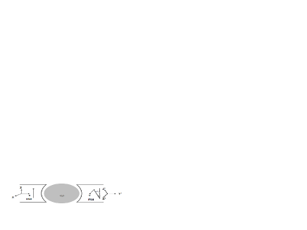
Figure 1: The schematic plot of the spin-degenerated quantum dot connected by two ferromagnetic leads. The magnetic moment of the left lead is always at $z$ direction and the magnetic moment of the right lead is at an angle $\theta_{R}$ with respect to the $z$-axis in the $x-z$ plane.

In the second quantized form, Hamiltonian is

$$\hat{H}=\hat{H}_{lead}+\hat{H}_{dot}+\hat{H}_{T},$$ (1)

where $\hat{H}_{lead}$ is the Hamiltonian of the leads,

$$\hat{H}_{lead}=\sum_{k_{\alpha}\sigma}(\epsilon_{k_{\alpha}}-\sigma M_{\alpha}cos\theta_{\alpha})\hat{C}^{\dagger}_{k_{\alpha}\sigma}\hat{C}_{k_{\alpha}\sigma}-\sum_{k_{\alpha}\sigma}M_{\alpha}sin\theta_{\alpha}\hat{C}^{\dagger}_{k_{\alpha}\sigma}\hat{C}_{k_{\alpha}\bar{\sigma}},$$ (2)

where $\hat{C}^{\dagger}_{k_{\alpha}\sigma}$ creates an electron in lead $\alpha$ with energy level $k$ and spin $\sigma$, $\sigma=\pm 1$ and $\bar{\sigma}=-\sigma$. The second term $\hat{H}_{dot}$ is the Hamiltonian of the isolated quantum dot,

$$\hat{H}_{dot}=\sum_{n\sigma}\epsilon_{n}\hat{d}^{\dagger}_{n\sigma}\hat{d}_{n\sigma},$$ (3)

The third term $\hat{H}_{T}$ is the Hamiltonian describing the coupling between quantum dot and the leads with the coupling constant $t_{k_{\alpha}n\sigma}$,

$$\hat{H}_{T}=\sum_{k_{\alpha}n\sigma}[t_{k_{\alpha}n\sigma}\hat{C}^{\dagger}_{k_{\alpha}\sigma}\hat{d}_{n\sigma}+c.c.],$$ (4)

where $c.c.$ denotes the complex conjugate. By applying the Bogoliubov transformation [44],

$$\hat{c}_{k_{\alpha}\sigma}=cos(\theta_{\alpha}/2)\hat{C}_{k_{\alpha}\sigma}-\sigma sin(\theta_{\alpha}/2)\hat{C}_{k_{\alpha}\bar{\sigma}},$$ (5)

we can diagonalize the Hamiltonian of the electrodes to give the following effective Hamiltonian,

$$\hat{H}_{\alpha}=\sum_{k\sigma}(\epsilon_{k_{\alpha}}-\sigma M_{\alpha})\hat{c}^{\dagger}_{k_{\alpha}\sigma}\hat{c}_{k_{\alpha}\sigma}.$$ (6)

So for a ferromagnetic lead coupled with scattering quantum dot, the line-width function $\Gamma_{\alpha}$ can be written as [45]

$$\Gamma_{\alpha}=R_{\alpha}\left(\begin{array}[]{ccc}\Gamma_{\alpha\uparrow}&0\\ 0&\Gamma_{\alpha\downarrow}\\ \end{array}\right)R^{\dagger}_{\alpha},$$ (9)

where

$$R_{\alpha}=\left(\begin{array}[]{ccc}cos\frac{\theta_{\alpha}}{2}&-sin\frac{\theta_{\alpha}}{2}\\ sin\frac{\theta_{\alpha}}{2}&cos\frac{\theta_{\alpha}}{2}\\ \end{array}\right)$$ (10)

is the rotational matrix.

The current operator of the lead $\alpha$ with spin $\sigma$ is defined as

$$\hat{I}_{\alpha\sigma}(t)=q\frac{d\hat{N}_{\alpha\sigma}}{dt}.$$ (11)

where $\hat{N}_{\alpha\sigma}=\sum_{k}\hat{C}^{\dagger}_{k_{\alpha}\sigma}\hat{C}_{k_{\alpha}\sigma}$ is the number operator for the electron in the lead $\alpha$. By using the Heisenberg equation of motion, we have

$$\hat{I}_{\alpha\sigma}(t)=-i\frac{q}{\hbar}\sum_{km}[t_{k_{\alpha}m\sigma}\hat{C}_{k_{\alpha}\sigma}^{\dagger}(t)\hat{d}_{m\sigma}(t)]+c.c.$$ (12)

The average current can be expressed by in terms of Green’s function,

$$<\hat{I}_{\alpha\sigma}(t)>=-\frac{q}{\hbar}\sum_{km}[t_{k_{\alpha}m\sigma}G^{<}_{m\sigma k_{\alpha}\sigma}(t,t)+c.c].$$ (13)

If we consider the total charge current flowing through the lead $\alpha$, the charge current operator can be expressed as

$$\hat{I}_{\alpha}=\hat{I}_{\alpha\uparrow}+\hat{I}_{\alpha\downarrow}$$ (14)

and the spin current operator in $z$-direction is

$$\hat{I}^{s}_{\alpha}=\frac{\hbar}{2}\frac{1}{q}(\hat{I}_{\alpha\uparrow}-\hat{I}_{\alpha\downarrow}).$$ (15)

Since the local spin current is not conserved, the loss of the spin angular momentum is transferred to the magnetization of the free layer. For spin transfer torque, we are interested in the MNM system and we assume that electron coming from the left lead which is pinned and the right lead is the free layer. The spin transfer torque can be calculated as follows. The total spin of the right ferromagnetic electrode is[46]

$$\hat{S}^{\theta}=\frac{\hbar}{2}\sum_{k_{R}\mu\nu}C_{k_{R}\mu}^{\dagger}C_{k\nu}(\mathcal{R}^{-1}\chi_{\mu})^{\dagger}\hat{\sigma}(\mathcal{R}^{-1}\chi_{\nu}).$$ (16)

Here, $\hat{\sigma}$ is Pauli matrices and the spinup state $\chi_{\mu(\nu)}=(\begin{array}[]{ccc}1\\ 0\end{array})$ for $\mu(\nu)=1$ or the spindown state $\chi_{\mu(\nu)}=(\begin{array}[]{ccc}0\\ 1\end{array})$ for $\mu(\nu)=-1$. Note that the equation above is written in $xyz$ coordinate frame while $\hat{S}^{\theta}$ are quantized in the $x^{\prime}y^{\prime}z^{\prime}$ frame. Because $\hat{S}^{\theta}(t)$ is along the direction of $z^{\prime}$, the total spin torque $\hat{\tau}=\frac{\partial\hat{S}^{\theta}}{\partial t}=\frac{i}{\hbar}[\hat{H}_{T},\hat{S}^{\theta}]$ should be along the direction of $x^{\prime}$ (see figure 1). So we need the expression of the spin operator of the right lead along $x^{\prime}$ direction, $\hat{S}^{\theta}_{x^{{}^{\prime}}}$, which can be obtained from equation (16),

$$\hat{S}^{\theta}_{x^{{}^{\prime}}}=\frac{\hbar}{2}\sum_{k_{R}\sigma}(\hat{C}^{\dagger}_{k_{R}\sigma}\hat{C}_{k_{R}\bar{\sigma}}cos\theta-\sigma\hat{C}^{\dagger}_{k_{R}\sigma}\hat{C}_{k_{R}\sigma}sin\theta).$$ (17)

According to the Heisenberg equation of motion, the spin transfer torque operator is

$$\hat{\tau}_{R} = \hat{\tau}_{x^{{}^{\prime}}}=\frac{i}{\hbar}[\hat{H}_{T},\hat{S}^{\theta}_{x{{}^{\prime}}}]$$ (18)

$$= -\frac{i}{2}[\sum_{k_{R}n\sigma\sigma^{{}^{\prime}}}(\hat{C}_{k_{R}\sigma}^{\dagger}\mathcal{R}_{\sigma\sigma^{{}^{\prime}}}\hat{d}_{n\sigma^{{}^{\prime}}}t_{k_{R}n\sigma^{{}^{\prime}}}-t_{k_{R}n\sigma^{{}^{\prime}}}^{*}\hat{d}_{n\sigma^{{}^{\prime}}}^{\dagger}\mathcal{R}_{\sigma\sigma^{{}^{\prime}}}\hat{C}_{k_{R}\sigma})]$$

where,

$$\mathcal{R}=\left(\begin{array}[]{ccc}\mathcal{R}_{\uparrow\uparrow}&\mathcal{R}_{\uparrow\downarrow}\\ \mathcal{R}_{\downarrow\uparrow}&\mathcal{R}_{\downarrow\downarrow}\\ \end{array}\right)=\left(\begin{array}[]{ccc}-sin\theta_{R}&cos\theta_{R}\\ cos\theta_{R}&sin\theta_{R}\\ \end{array}\right),t_{k_{R}n}=\left(\begin{array}[]{ccc}t_{k_{R}n\uparrow}&0\\ 0&t_{k_{R}n\downarrow}\\ \end{array}\right).$$ (19)

The average spin transfer torque is[46]

$$<\hat{\tau}_{R}> = Re\{\sum_{k_{R}n}Tr_{\sigma}[t_{k_{R}n}\mathcal{R}G_{n,k_{R}}^{<}]\}$$ (20)

$$= \int\frac{dE}{2\pi}(f_{L}-f_{R})Tr[G^{r}\Gamma_{L}G^{a}(i\Sigma_{R}^{a}\mathcal{R}-i\mathcal{R}\Sigma_{R}^{r})]$$

where $Tr_{\sigma}$ is over spin space.

The correlation of the charge current is given by

$$<\Delta\hat{I}_{\alpha}(t_{1})\Delta\hat{I}_{\beta}(t_{2})>=\sum_{\sigma\sigma{{}^{\prime}}}(<\Delta\hat{I}_{\alpha\sigma}(t_{1})\Delta\hat{I}_{\beta\sigma{{}^{\prime}}}(t_{2})>)$$ (21)

and the shot noise of spin current is

$$<\Delta\hat{I}^{s}_{\alpha}(t_{1})\Delta\hat{I}^{s}_{\beta}(t_{2})>=\frac{1}{4}\frac{\hbar^{2}}{q^{2}}\sum_{\sigma\sigma{{}^{\prime}}}\sigma\sigma{{}^{\prime}}(<\Delta\hat{I}_{\alpha\sigma}(t_{1})\Delta\hat{I}_{\beta\sigma{{}^{\prime}}}(t_{2})>)$$ (22)

where

$$\Delta\hat{I}_{\alpha\sigma}=\hat{I}_{\alpha\sigma}-<\hat{I}_{\alpha\sigma}>,$$ (23)

and $\sigma=\uparrow\downarrow$ or $\pm 1$. Finally, the correlation of spin transfer torque is

$${\cal S}(t_{1},t_{2})=<\Delta\hat{\tau}_{R}(t_{1})\Delta\hat{\tau}_{R}(t_{2})>,$$ (24)

where $\Delta\hat{\tau}_{R}={\hat{\tau}}_{R}-<{\hat{\tau}_{R}}>$.

We now derive the correlation of charge current, spin current, and spin transfer torque. Clearly, all correlation functions contain the following term,

$$<\hat{I}_{\alpha\sigma}(t_{1})\hat{I}_{\beta\sigma{{}^{\prime}}}(t_{2})>=-\frac{q^{2}}{\hbar^{2}}\sum_{kk{{}^{\prime}}mn}$$

$$[t_{k_{\alpha}m\sigma}t_{k^{\prime}_{\beta}n\sigma{{}^{\prime}}}<\hat{C}^{\dagger}_{k_{\alpha}\sigma}(t_{1})\hat{d}_{m\sigma}(t_{1})\hat{C}^{\dagger}_{k^{\prime}_{\beta}\sigma{{}^{\prime}}}(t_{2})\hat{d}_{n\sigma{{}^{\prime}}}(t_{2})>$$

$$+t^{\ast}_{k_{\alpha}m\sigma}t^{\ast}_{k^{\prime}_{\beta}n\sigma{{}^{\prime}}}<\hat{d}^{\dagger}_{m\sigma}(t_{1})\hat{C}_{k_{\alpha}\sigma}(t_{1})\hat{d}^{\dagger}_{n\sigma{{}^{\prime}}}(t_{2})\hat{C}_{k^{\prime}_{\beta}\sigma{{}^{\prime}}}(t_{2})>$$

$$-t_{k_{\alpha}m\sigma}t^{\ast}_{k^{\prime}_{\beta}n\sigma{{}^{\prime}}}<\hat{C}^{\dagger}_{k_{\alpha}\sigma}(t_{1})\hat{d}_{m\sigma}(t_{1})\hat{d}^{\dagger}_{n\sigma{{}^{\prime}}}(t_{2})\hat{C}_{k^{\prime}_{\beta}\sigma{{}^{\prime}}}(t_{2})>$$

$$-t^{\ast}_{k_{\alpha}m\sigma}t_{k^{\prime}_{\beta}n\sigma{{}^{\prime}}}<\hat{d}^{\dagger}_{m\sigma}(t_{1})\hat{C}_{k_{\alpha}\sigma}(t_{1})\hat{C}^{\dagger}_{k^{\prime}_{\beta}\sigma{{}^{\prime}}}(t_{2})\hat{d}_{n\sigma{{}^{\prime}}}(t_{2})>],$$

(25)

and

$$<\hat{I}_{\alpha\sigma}(t_{1})><\hat{I}_{\beta\sigma{{}^{\prime}}}(t_{2})>=-\frac{q^{2}}{\hbar^{2}}\sum_{kk{{}^{\prime}}mn}$$

$$[t_{k_{\alpha}m\sigma}t_{k^{\prime}_{\beta}n\sigma{{}^{\prime}}}<\hat{C}^{\dagger}_{k_{\alpha}\sigma}(t_{1})\hat{d}_{m\sigma}(t_{1})><\hat{C}^{\dagger}_{k^{\prime}_{\beta}\sigma{{}^{\prime}}}(t_{2})\hat{d}_{n\sigma{{}^{\prime}}}(t_{2})>$$

$$+t^{\ast}_{k_{\alpha}m\sigma}t^{\ast}_{k^{\prime}_{\beta}n\sigma{{}^{\prime}}}<\hat{d}^{\dagger}_{m\sigma}(t_{1})\hat{C}_{k_{\alpha}\sigma}(t_{1})><\hat{d}^{\dagger}_{n\sigma{{}^{\prime}}}(t_{2})\hat{C}_{k^{\prime}_{\beta}\sigma{{}^{\prime}}}(t_{2})>$$

$$-t_{k_{\alpha}m\sigma}t^{\ast}_{k^{\prime}_{\beta}n\sigma{{}^{\prime}}}<\hat{C}^{\dagger}_{k_{\alpha}\sigma}(t_{1})\hat{d}_{m\sigma}(t_{1})><\hat{d}^{\dagger}_{n\sigma{{}^{\prime}}}(t_{2})\hat{C}_{k^{\prime}_{\beta}\sigma{{}^{\prime}}}(t_{2})>$$

$$-t^{\ast}_{k_{\alpha}m\sigma}t_{k^{\prime}_{\beta}n\sigma{{}^{\prime}}}<\hat{d}^{\dagger}_{m\sigma}(t_{1})\hat{C}_{k_{\alpha}\sigma}(t_{1})><\hat{C}^{\dagger}_{k^{\prime}_{\beta}\sigma{{}^{\prime}}}(t_{2})\hat{d}_{n\sigma{{}^{\prime}}}(t_{2})>].$$

(26)

Using the Wick’s theorem [47], we have,

$$<\hat{C}_{k_{\alpha}\sigma}^{\dagger}(t_{1})\hat{d}_{m\sigma}(t_{1})\hat{C}_{k^{\prime}_{\beta}\sigma{{}^{\prime}}}^{\dagger}(t_{2})\hat{d}_{n\sigma{{}^{\prime}}}(t_{2})>$$

$$=<\hat{C}_{k_{\alpha}\sigma}^{\dagger}(t_{1})\hat{d}_{m\sigma}(t_{1})><\hat{C}_{k^{\prime}_{\beta}\sigma{{}^{\prime}}}^{\dagger}(t_{2})\hat{d}_{n\sigma{{}^{\prime}}}(t_{2})>$$

$$+<\hat{C}_{k_{\alpha}\sigma}^{\dagger}(t_{1})\hat{d}_{n\sigma{{}^{\prime}}}(t_{2})><\hat{d}_{m\sigma}(t_{1})\hat{C}_{k^{\prime}_{\beta}\sigma{{}^{\prime}}}^{\dagger}(t_{2})>.$$ (27)

The shot noise can be expressed in terms of Green’s function

$$<\Delta\hat{I}_{\alpha\sigma}(t_{1})\Delta\hat{I}_{\beta\sigma{{}^{\prime}}}(t_{2})>=$$

$$-\frac{q^{2}}{\hbar^{2}}\sum_{kk{{}^{\prime}}mn}[t_{k_{\alpha}m\sigma}t_{k^{\prime}_{\beta}n\sigma{{}^{\prime}}}G^{>}_{m\sigma k^{\prime}_{\beta}\sigma{{}^{\prime}}}G^{<}_{n\sigma{{}^{\prime}}k_{\alpha}\sigma}$$

$$+t^{\ast}_{k_{\alpha}m\sigma}t^{\ast}_{k^{\prime}_{\beta}n\sigma{{}^{\prime}}}G^{>}_{k_{\alpha}\sigma n\sigma{{}^{\prime}}}G^{<}_{k^{\prime}_{\beta}\sigma m\sigma}$$

$$-t_{k_{\alpha}m\sigma}t^{\ast}_{k^{\prime}_{\beta}n\sigma{{}^{\prime}}}G^{>}_{m\sigma n\sigma{{}^{\prime}}}G^{<}_{k^{\prime}_{\beta}\sigma{{}^{\prime}}k_{\alpha}\sigma}$$

$$-t^{\ast}_{k_{\alpha}m\sigma}t_{k^{\prime}_{\beta}n\sigma{{}^{\prime}}}G^{>}_{k_{\alpha}\sigma k^{\prime}_{\beta}\sigma{{}^{\prime}}}G^{<}_{n\sigma{{}^{\prime}}m\sigma}].$$ (28)

From the Langreth theorem of analytic continuation, we have

$$G^{<,>}_{m\sigma k^{\prime}_{\beta}\sigma{{}^{\prime}}}(t_{1},t_{2})$$ (29)

$$= \sum_{p\sigma_{p}}\int dt[G^{r}_{m\sigma p\sigma_{p}}(t_{1},t)t^{*}_{k^{\prime}_{\beta}p\sigma_{p}}g^{<,>}_{k^{\prime}_{\beta}\sigma_{p}\sigma{{}^{\prime}}}(t,t_{2})$$

$$+ G^{<,>}_{m\sigma p\sigma_{p}}(t_{1},t)t^{*}_{k^{\prime}_{\beta}p\sigma_{p}}g^{a}_{k^{\prime}_{\beta}\sigma_{p}\sigma{{}^{\prime}}}(t,t_{2})],$$

and

$$G^{<,>}_{k^{\prime}_{\beta}\sigma{{}^{\prime}}m\sigma}(t_{1},t_{2})$$ (30)

$$= \sum_{p\sigma_{p}}\int dt[g^{<,>}_{k^{\prime}_{\beta}\sigma{{}^{\prime}}\sigma_{p}}(t_{1},t)t_{k^{\prime}_{\beta}p\sigma_{p}}G^{a}_{p\sigma_{p}m\sigma}(t_{1},t)$$

$$+ g^{r}_{k^{\prime}_{\beta}\sigma{{}^{\prime}}\sigma_{p}}(t_{1},t)t_{k^{\prime}_{\beta}p\sigma_{p}}G^{<,>}_{p\sigma_{p}m\sigma}(t,t_{2})],$$

as well as

$$G^{<,>}_{k_{\alpha}\sigma k^{\prime}_{\beta}\sigma{{}^{\prime}}}(t_{1},t_{2})=g^{<,>}_{k^{\prime}_{\beta}\sigma\sigma{{}^{\prime}}}(t_{1},t_{2})\delta_{kk^{\prime}}\delta_{\alpha\beta}$$ (31)

$$+ \sum_{p\sigma_{p}}\int dt[G^{r}_{k_{\alpha}\sigma p\sigma_{p}}(t_{1},t)t^{*}_{k^{\prime}_{\beta}p\sigma_{p}}g^{<,>}_{k^{\prime}_{\beta}\sigma_{p}\sigma{{}^{\prime}}}(t,t_{2})$$

$$+ G^{<,>}_{k_{\alpha}\sigma p\sigma_{p}}(t_{1},t)t^{*}_{k^{\prime}_{\beta}p\sigma_{p}}g^{a}_{k^{\prime}_{\beta}\sigma_{p}\sigma{{}^{\prime}}}(t,t_{2})],$$

The self-energy is given by

$$\Sigma^{\gamma}_{\alpha m\sigma n\sigma{{}^{\prime}}}(t_{1},t_{2})=\sum_{k}t^{*}_{k_{\alpha}m\sigma}(t_{1})g^{\gamma}_{k_{\alpha}\sigma\sigma{{}^{\prime}}}(t_{1},t_{2})t_{k_{\alpha}n\sigma{{}^{\prime}}}(t_{2}).$$ (32)

From the above equations, we can calculate the noise spectrum $S$ defined as follows [6]:

$$\pi\delta(0)S_{\alpha\beta}^{\sigma\sigma{{}^{\prime}}}=\int dt_{1}dt_{2}<\Delta\hat{I}_{\alpha\sigma}(t_{1})\Delta\hat{I}_{\beta\sigma{{}^{\prime}}}(t_{2})>.$$ (33)

Using Eqs.(29)-(32), it is straightforward to write the noise spectrum as

$$S_{\alpha\beta}^{\sigma\sigma{{}^{\prime}}}=\sum_{i=0}^{4}S_{i,\alpha\beta}^{\sigma\sigma{{}^{\prime}}}.$$ (34)

Here

$$\pi\delta(0)S_{0,\alpha\beta}^{\sigma\sigma{{}^{\prime}}}=\frac{q^{2}}{\hbar^{2}}\delta_{\alpha\beta}Tr_{t}[{G^{>}_{\sigma\sigma{{}^{\prime}}}}\Sigma^{<}_{\alpha,\sigma{{}^{\prime}}\sigma}+{\Sigma^{>}_{\alpha,\sigma\sigma{{}^{\prime}}}}G^{<}_{\sigma{{}^{\prime}}\sigma}],$$ (35)

$$\pi\delta(0)S_{1,\alpha\beta}^{\sigma\sigma{{}^{\prime}}}= -\frac{q^{2}}{\hbar^{2}}Tr_{t}[(G^{r}\Sigma^{>}_{\beta}+G^{>}\Sigma^{a}_{\beta})_{\sigma\sigma{{}^{\prime}}}$$ (36)

$$\times(G^{r}\Sigma^{<}_{\alpha}+G^{<}\Sigma^{a}_{\alpha})_{\sigma{{}^{\prime}}\sigma}],$$

$$\pi\delta(0)S_{2,\alpha\beta}^{\sigma\sigma{{}^{\prime}}}= -\frac{q^{2}}{\hbar^{2}}Tr_{t}[(\Sigma^{>}_{\alpha}G^{a}+\Sigma^{r}_{\alpha}G^{>})_{\sigma\sigma{{}^{\prime}}}$$ (37)

$$\times(\Sigma^{<}_{\beta}G^{a}+\Sigma^{r}_{\beta}G^{<})_{\sigma{{}^{\prime}}\sigma}],$$

$$\pi\delta(0)S_{3,\alpha\beta}^{\sigma\sigma{{}^{\prime}}}= \frac{q^{2}}{\hbar^{2}}Tr_{t}[G^{>}_{\sigma\sigma{{}^{\prime}}}(\Sigma^{r}_{\beta}G^{r}\Sigma^{<}_{\alpha}+\Sigma^{<}_{\beta}G^{a}\Sigma^{a}_{\alpha}$$ (38)

$$+\Sigma^{r}_{\beta}G^{<}\Sigma^{a}_{\alpha})_{\sigma{{}^{\prime}}\sigma})],$$

$$\pi\delta(0)S_{4,\alpha\beta}^{\sigma\sigma{{}^{\prime}}}= \frac{q^{2}}{\hbar^{2}}Tr_{t}[(\Sigma^{r}_{\alpha}G^{r}\Sigma^{>}_{\beta}+\Sigma^{>}_{\alpha}G^{a}\Sigma^{a}_{\beta}$$ (39)

$$+\Sigma^{r}_{\alpha}G^{>}\Sigma^{a}_{\beta})_{\sigma\sigma{{}^{\prime}}}G^{<}_{\sigma{{}^{\prime}}\sigma}].$$

Since all Green’s functions depend on double time indices, the trace $Tr_{t}$ is taken in the time domain.

To get the charge current noise spectrum, we combine equation (21) with equation (33) and perform Fourier transformation, the well known auto charge current noise can be obtained

$$S_{LL}=\frac{q^{2}}{\pi}\int dE(f_{L}-f_{R})^{2}Tr[(1-T)T],$$ (40)

here, $T=\Gamma_{L}G^{r}\Gamma_{R}G^{a}$ is the transmission matrix. We can also get the cross charge current shot noise (along z direction):

$$S_{LR}=-\frac{q^{2}}{\pi}\int dE(f_{L}-f_{R})^{2}Tr[(1-T)T],$$ (41)

$S_{LL}+S_{LR}=0$ confirms the current conservation.

For spin current noise spectrum, the situation is very different. We combine equation (22) with equation (33), taking Fourier transformation, and using the relation

$$\sum_{\sigma\sigma{{}^{\prime}}}\sigma\sigma{{}^{\prime}}A_{\sigma\sigma{{}^{\prime}}}B_{\sigma{{}^{\prime}}\sigma}=Tr[A\sigma_{z}B\sigma_{z}],$$ (42)

($\sigma_{z}$ is pauli matrix), we can obtain the auto spin current shot noise (zero-temperature limit),

$$S^{\sigma}_{LL}=\frac{\hbar^{2}}{4\pi}\int dE(f_{L}-f_{R})^{2}Tr[\sigma_{z}T\sigma_{z}(1-T)].$$ (43)

Similarly, the cross spin current shot noise can be obtained:

$$S^{\sigma}_{LR}=-\frac{\hbar^{2}}{4\pi}\int dE(f_{R}-f_{L})^{2}Tr\{[G^{r}\Gamma_{R}G^{a}(\Sigma^{a}_{R}\sigma_{z}$$

$$-\sigma_{z}\Sigma^{r}_{R})+G^{r}\Gamma_{R}\sigma_{z}](G^{r}\Gamma_{L}\sigma_{z}+G^{r}\Gamma_{L}G^{a}(\Sigma_{L}^{a}\sigma_{z}$$

$$-\sigma_{z}\Sigma_{L}^{r})\}.$$ (44)

Now, we derive the shot noise of spin transfer torque ${\cal S}(t_{1},t_{2})$,

$${\cal S}(t_{1},t_{2}) =-\frac{1}{4}<\sum_{k_{R_{A}}n}\sum_{\sigma_{A}\sigma_{A}^{{}^{\prime}}}(\hat{C}_{k_{R_{A}}\sigma_{A}}^{\dagger}\mathcal{R}_{\sigma_{A}\sigma_{A}^{{}^{\prime}}}\hat{d}_{n\sigma^{{}^{\prime}}_{A}}t_{k_{R_{A}}n\sigma^{{}^{\prime}}_{A}}-t_{k_{R_{A}}n\sigma^{{}^{\prime}}_{A}}^{*}\hat{d}_{n\sigma^{{}^{\prime}}_{A}}^{\dagger}\mathcal{R}_{\sigma_{A}\sigma_{A}^{{}^{\prime}}}\hat{C}_{k_{R_{A}}\sigma_{A}})$$ (45)

$$\sum_{k_{R_{B}}m}\sum_{\sigma_{B}\sigma_{B}^{{}^{\prime}}}(\hat{C}_{k_{R_{B}}\sigma_{B}}^{\dagger}\mathcal{R}_{\sigma_{B}\sigma_{B}^{{}^{\prime}}}\hat{d}_{n\sigma^{{}^{\prime}}_{B}}t_{k_{R_{B}}n\sigma^{{}^{\prime}}_{B}}-t_{k_{R_{B}}n\sigma^{{}^{\prime}}_{B}}^{*}\hat{d}_{n\sigma^{{}^{\prime}}_{B}}^{\dagger}\mathcal{R}_{\sigma_{B}\sigma_{B}^{{}^{\prime}}}\hat{C}_{k_{R_{B}}\sigma_{B}})>$$

and

$$<\hat{\tau}_{R}(t)>=\frac{i}{2}<\sum_{k_{R_{A}}n}\sum_{\sigma_{A}\sigma_{A}^{{}^{\prime}}}(\hat{C}_{k_{R_{A}}\sigma_{A}}^{\dagger}\mathcal{R}_{\sigma_{A}\sigma_{A}^{{}^{\prime}}}\hat{d}_{n\sigma^{{}^{\prime}}_{A}}t_{k_{R_{A}}n\sigma^{{}^{\prime}}_{A}}-t_{k_{R_{A}}n\sigma^{{}^{\prime}}_{A}}^{*}\hat{d}_{n\sigma^{{}^{\prime}}_{A}}^{\dagger}\mathcal{R}_{\sigma_{A}\sigma_{A}^{{}^{\prime}}}\hat{C}_{k_{R_{A}}\sigma_{A}})>.$$ (46)

Similarly, we define the shot noise spectrum of spin transfer torque like the shot noise of spin current, it can be written as

$$\pi\delta(0)S^{\tau} = \int dt_{1}dt_{2}{\cal S}(t_{1},t_{2}).$$ (47)

where ${\cal S}(t_{1},t_{2})$ is defined in equation (24).

By using the Wick’s theorem, and after Fourier transformation, we can obtain expression of $S^{\tau}$,

$$S^{\tau}= \frac{\hbar^{2}}{4\pi}\int dE(f_{L}-f_{R})\{Tr[G^{r}\Gamma_{L}G^{a}\mathcal{R}\Gamma_{R}\mathcal{R}$$

$$+ G^{r}\Gamma_{L}G^{a}(\Sigma_{R}^{a}\mathcal{R}-\mathcal{R}\Sigma_{R}^{r})G^{r}\Gamma_{L}G^{a}(\Sigma_{R}^{a}\mathcal{R}-\mathcal{R}\Sigma_{R}^{r})$$

$$+ G^{r}(i\mathcal{R}\Sigma_{R}^{r}-i\Sigma_{R}^{a}\mathcal{R}-\Gamma_{R}\mathcal{R})G^{r}\Gamma_{L}G^{a}(\Sigma_{R}^{a}\mathcal{R}-\mathcal{R}\Sigma_{R}^{r})$$

$$+ (\Sigma_{R}^{a}\mathcal{R}-\mathcal{R}\Sigma_{R}^{r})G^{r}\Gamma_{L}G^{a}(\mathcal{R}\Gamma_{R}-i\mathcal{R}\Sigma_{R}^{r}+i\Sigma_{R}^{a}\mathcal{R})G^{a}]\}.$$ (48)

3 Shot noise of spin current and spin torque for MNM system

In this paper, we consider a normal quantum dot connected by two ferromagnetic leads (see figure 1) (MNM system). The magnetic moment of left lead is pointing to the $z$-direction, while the moment of right lead is at an angle $\theta_{R}$ to the $z$-axis in the $x-z$ plane. Hence the Hamiltonian of quantum dot can be written as

$$H_{dot}=\left(\begin{array}[]{ccc}\epsilon_{0}&0\\ 0&\epsilon_{0}\\ \end{array}\right).$$ (49)

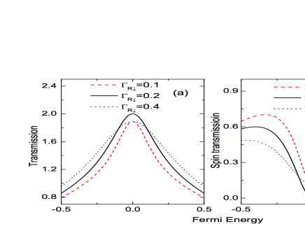
Figure 2: (a)The charge transmission coefficient $(T_{\uparrow}+T_{\downarrow})$ and (b)the spin transmission coefficient $(T_{\uparrow}-T_{\downarrow})$ versus fermi energy when $\Gamma_{R\downarrow}=0.1$ (red dashed line), $\Gamma_{R\downarrow}=0.2$ (black solid line), $\Gamma_{R\downarrow}=0.4$ (blue dotted line). The other parameters are $\theta_{R}=0$, $\epsilon=0$ $\Gamma_{L\downarrow}=0.2$, $\Gamma_{L\uparrow}=\Gamma_{R\uparrow}=0.8$. The energy unit is eV.

Firstly, we set the direction of magnetization of the right lead be along the $z$ direction, i.e., let $\theta_{R}=0$ and calculate the charge and spin current according to Landauer-B$\ddot{u}$ttiker formula

$$I_{c}=-\frac{q}{\hbar}\int\frac{dE}{2\pi}Tr[\hat{T}(E)](f_{L}-f_{R}),$$ (50)

and the expression of spin current is

$$I_{s}=\frac{1}{2}\int\frac{dE}{2\pi}Tr[\sigma_{z}\hat{T}(E)](f_{L}-f_{R}).$$ (51)

The charge and spin transmission coefficients are depicted in figure 2. In the calculation, we have chosen $\Gamma_{L\uparrow}=\Gamma_{R\uparrow}=0.8$eV and fix the energy unit is to be eV. Let $\Gamma_{L\downarrow}=\Gamma_{R\downarrow}=0.2$eV (Here, we let $\Gamma_{\alpha\uparrow}\neq\Gamma_{\alpha\downarrow}$ due to the presence of ferromagnetic leads), we found that the charge transmission coefficient reaches two at the resonant energy level $E=\epsilon_{0}$ of the quantum dot (solid line in the left panel of figure 2), while the spin transmission coefficient is zero at resonant energy point (solid line in the right panel of figure 2). For parallel situation ($\theta_{R}=0$) there is no spin flip so that different spin channel can be treated separately. For a symmetric coupling from the lead, both spin up and spin down electrons have complete transmission at the resonance. For total charge current they add up together while for total spin current they cancel to each other. When we break this symmetry and change $\Gamma_{R\downarrow}$ while keeping $\Gamma_{L\downarrow}$ constant, the spin down transport will be partially blocked, so the charge transmission coefficient will decrease and the spin transmission coefficient will increase (see the dashed lines and dotted lines in figure 2).

Figure 3 gives a comparison between the charge current and spin current versus $\theta_{R}$ under the small bias voltage 0.05V. From the figure, we find that for the symmetric coupling with $\Gamma_{L\uparrow}=\Gamma_{R\uparrow}$ and $\Gamma_{L\downarrow}=\Gamma_{R\downarrow}$, both charge current and spin current decrease as $\theta_{R}$ increasing from zero to $\pi$ (see the solid lines in figure 3(a) and 3(b)). But if we fix $\Gamma_{L\downarrow}$ and change $\Gamma_{R\downarrow}$, although the charge current still decreases when $\theta_{R}$ changes from zero to $\pi$, the spin current increases when $\Gamma_{R\downarrow}>\Gamma_{L\downarrow}$ and decreases when $\Gamma_{R\downarrow}<\Gamma_{L\downarrow}$ and changes sign at $\theta_{R}=\pi$. To understand the behavior, we plot the spin-up current in the panel (c) and spin-down current in the panel (d), respectively. One can clearly see that spin up current always decreases with $\theta_{R}$ from zero to $\pi$, but spin down current always increases though it is negative. So the competition between spin up and down channels determines how the total spin current varies with $\Gamma_{R\downarrow}$. Another interesting result is that at $\theta_{R}=\pi$, i.e., when the magnetic moments of the two leads are antiparallel, the spin down current does not change when we change the $\Gamma_{R\downarrow}$ (see figure 4(d)) while keeping other parameters the same. In fact, when we change the $\Gamma_{R\downarrow}$ at $\theta_{R}=\pi$, we actually change the right coupling line-width constant of spin up but not spin down due to $\Gamma_{R}(\pi)=R_{\alpha}(\pi)\left(\begin{array}[]{ccc}\Gamma_{R\uparrow}&0\\ 0&\Gamma_{R\downarrow}\\ \end{array}\right)R^{\dagger}_{\alpha}(\pi)=\left(\begin{array}[]{ccc}\Gamma_{R\downarrow}&0\\ 0&\Gamma_{R\uparrow}\\ \end{array}\right)$. So we can find that at $\theta_{R}=\pi$, the spin up current is different with different $\Gamma_{R\downarrow}$ but spin down keeps unchanged.

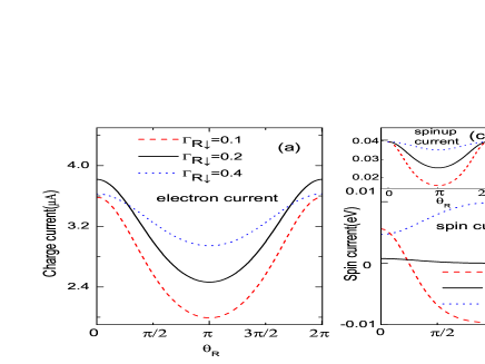
Figure 3: The charge current (panel (a)), total spin current (panel (b)), spin up current (panel (c)) and spin down current (panel (d)) versus $\theta_{R}$ for MNM system at $\Gamma_{R\downarrow}=0.1$ (red dashed line), $\Gamma_{R\downarrow}=0.2$ (black solid line), $\Gamma_{R\downarrow}=0.4$ (blue dotted line),respectively. The other parameters are $V_{bias}=0.05$V, $\epsilon_{0}=0$, $\Gamma_{L\uparrow}=\Gamma_{R\uparrow}=0.8$, $\Gamma_{L\downarrow}=0.2$.

To study the shot noise of spin current, we first examine the differential shot noise spectrum versus bias voltage $V_{L}=V$ and $V_{R}=0$. At zero temperature, they can be calculated from equations (43) and (44) (AC means auto-correlation and CC means cross-correlation)

$$N_{AC}=\frac{4\pi}{q\hbar^{2}}\frac{\partial S_{LL}^{\sigma_{z}}}{\partial V}=Tr[\sigma_{z}T(E)\sigma_{z}(1-T(E))]|_{E=qV}$$ (52)

and

$$N_{CC}=\frac{4\pi}{q\hbar^{2}}\frac{\partial S_{LR}^{\sigma_{z}}}{\partial V}=-Tr\{[G^{r}\Gamma_{R}G^{a}(\Sigma^{a}_{R}\sigma_{z}-\sigma_{z}\Sigma^{r}_{R})+$$

$$G^{r}\Gamma_{R}\sigma_{z}](G^{r}\Gamma_{L}\sigma_{z}+G^{r}\Gamma_{L}G^{a}(\Sigma_{L}^{a}\sigma_{z}-\sigma_{z}\Sigma_{L}^{r}))\}|_{E=qV}.$$ (53)

For equation (53), we see that if the direction of magnetic moments of both leads are parallel the off-diagonal matrix elements of all the physical quantity including the linewidth function $\Gamma_{\alpha\sigma}$ are zero, so $\sigma_{z}$ commutes with other matrices in equation (53). Using this property and $G^{a}-G^{r}=iG^{r}\Gamma_{L}G^{a}+iG^{r}\Gamma_{R}G^{a}$, we find

$$N_{CC}=-Tr[\sigma_{z}T\sigma_{z}(I-T)]=-N_{AC}.$$ (54)

Figure 4: MNM system. (a) $N_{AC}$ of spin current noise versus the angle $\theta_{R}$ with $V_{bias}=0.05$V; (b) $N_{AC}$ versus the bias voltage with two electrode magnetic moments parallel; (c) $N_{AC}$versus the bias voltage with two electrode magnetic moments antiparallel. The other parameters are $\epsilon_{0}=0$, and $\Gamma_{L\uparrow}=\Gamma_{R\uparrow}=0.8,\Gamma_{L\downarrow}=\Gamma_{R\downarrow}=0.2$.

Now we calculate $N_{AC}$ from equations (52). The figure 4(a) gives $N_{AC}$ versus $\theta_{R}$. One can find that the differential spin shot $N_{AC}$ is small for parallel situation and reaches maximum when the magnetization of leads are antiparallel. We also plot differential spin shot noise versus bias voltage at parallel and antiparallel configurations in figure 4(b) and 4(c). When the magnetization of two lead are parallel, $N_{AC}$ increases abruptly with the bias voltage and reaches a flat plateau between about $V_{bias}=(0.3,0.7)V$, then decreases gradually upon further increasing bias voltage. However, for antiparallel case, $N_{AC}$ starts at a large value compared with that of parallel case and increases a bit to a maximum value at $V_{bias}=\pm 0.26V$. For large bias voltage $V_{bias}$ $N_{AC}$ decreases and gradually approaches to zero. We have shown that $N_{AC}+N_{CC}=0$ in the case of parallel and anti-parallel situations. It is found that this relation is still valid when $\theta_{R}$ is not equal to $0$ or $\pi$. In general, the relation $N_{AC}+N_{CC}$ is not satisfied. For instance, If we study a system MNMNM with three ferromagnetic layers or the MM interface where coupling matrix elements $\Gamma_{\sigma\bar{\sigma}}\neq 0$, one can get $N_{AC}+N_{CC}\neq 0$.

Now we analyze the spin transfer torque and its auto-correlation function. From equations (20) and (2), we calculate the derivative of spin transfer torque and its correlation function with respect to the bias voltage as follows:

$$T_{\tau}=\frac{2\pi}{q}\frac{\partial<\hat{\tau}_{R}>}{\partial V}=Tr[G^{r}\Gamma_{L}G^{a}(i\Sigma_{R}^{a}\mathcal{R}-i\mathcal{R}\Sigma_{R}^{r})]|_{E=qV},$$ (55)

and

$$N_{\tau} = \frac{4\pi}{q\hbar^{2}}\frac{\partial S^{\tau}}{\partial V}=Tr[G^{r}\Gamma_{L}G^{a}(\Sigma_{R}^{a}\mathcal{R}-\mathcal{R}\Sigma_{R}^{r})G^{r}\Gamma_{L}G^{a}(\Sigma_{R}^{a}\mathcal{R}-\mathcal{R}\Sigma_{R}^{r})$$ (56)

$$+ G^{r}\Gamma_{L}G^{a}\mathcal{R}\Gamma_{R}\mathcal{R}$$

$$+ G^{r}(i\mathcal{R}\Sigma_{R}^{r}-i\Sigma_{R}^{a}\mathcal{R}-\Gamma_{R}\mathcal{R})G^{r}\Gamma_{L}G^{a}(\Sigma_{R}^{a}\mathcal{R}-\mathcal{R}\Sigma_{R}^{r})$$

$$+ (\Sigma_{R}^{a}\mathcal{R}-\mathcal{R}\Sigma_{R}^{r})G^{r}\Gamma_{L}G^{a}(\mathcal{R}\Gamma_{R}-i\mathcal{R}\Sigma_{R}^{r}+i\Sigma_{R}^{a}\mathcal{R})G^{a}]\}|_{E=qV}.$$

Since most of calculations for the spin transfer torque were obtained using the formula[48, 49, 50] $\tau_{0}=\frac{I^{s}(\pi)-I^{s}(0)}{2}\sin\theta$, we also calculate $T^{\prime}_{\tau}=\frac{2\pi}{q}\frac{\partial\tau_{0}}{\partial V}$ for comparison. In figure 5, we plot $T_{\tau}$ and $T^{\prime}_{\tau}$ versus $\theta_{R}$. When the bias voltage is tuned far away from the resonant point $\epsilon_{0}$ (figure 5(a)), the profile of $T_{\tau}$ versus $\theta_{R}$ obeys $\sin\theta_{R}$ function. This gives very good agreement with $T^{\prime}_{\tau}$ which is expected since $T^{\prime}_{\tau}$ was derived for a non-resonant tunneling system. When the system is near resonance, however, $T_{\tau}$ deviates away from the sinusoidal dependence[46, 51]. This behavior can be understood as follows. When we set $\Gamma_{L\uparrow}=\Gamma_{R\uparrow}=\Gamma_{\uparrow}$ and $\Gamma_{L\downarrow}=\Gamma_{R\downarrow}=\Gamma_{\downarrow}$, equation (55) can be simplified as

$$T_{\tau}=\frac{1}{2}\frac{(qV-\epsilon_{0})^{2}(\Gamma_{\uparrow}^{2}-\Gamma_{\downarrow}^{2})\sin\theta}{(qV-\epsilon_{0})^{2}(\Gamma_{\uparrow}+\Gamma_{\downarrow})^{2}+[(qV-\epsilon_{0})^{2}-\Gamma_{\uparrow}\Gamma_{\downarrow}-\frac{1}{4}(\Gamma_{\uparrow}-\Gamma_{\downarrow})^{2}\sin^{2}\frac{\theta}{2}]^{2}}.$$ (57)

We examine the denominator of this equation. Since $\Gamma_{\uparrow}\neq\Gamma_{\downarrow}$, it is clear that near the resonance $qV\sim\epsilon_{0}$, the term $\sin^{2}(\theta/2)$ in the denominator cannot be neglected so that $T_{\tau}$ in the upper panel of figure (5) is not the $\sin\theta_{R}$ dependence. But when $|{qV-\epsilon_{0}}|$ is large enough so that the term $\sin^{2}(\theta/2)$ is small compared with the term $(qV-\epsilon_{0})^{2}$,we obtain $T_{\tau}\approx T^{\prime}_{\tau}$. Actually, we can derive $T^{\prime}_{\tau}$ by differentiating $I^{s}(\pi)$ and $I^{s}(0)$ according to equation (51) and obtain

$$T^{\prime}_{\tau}=\frac{1}{2}\frac{(qV-\epsilon_{0})^{2}(\Gamma_{\uparrow}^{2}-\Gamma_{\downarrow}^{2})\sin\theta}{[(qV-\epsilon_{0})^{2}+\Gamma_{\uparrow}^{2}][(qV-\epsilon_{0})^{2}+\Gamma_{\downarrow}^{2}]}.$$ (58)

One can easily find that if we neglect the term $\sin^{2}(\theta/2)$ in the denominator of $T_{\tau}$, $T_{\tau}$ will equal $T^{\prime}_{\tau}$.

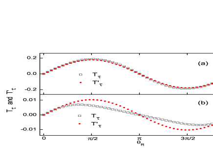
Figure 5: $T_{\tau}$ and $T^{\prime}_{\tau}$ versus $\theta_{R}$ with different bias voltages $V=0.01V$ (panel (a)) and $V=0.97V$ (panel (b)). The other parameters are $\epsilon_{0}=1.0$, $\Gamma_{L\uparrow}=\Gamma_{R\uparrow}=0.8,\Gamma_{L\downarrow}=\Gamma_{R\downarrow}=0.2$.

Figure 6: $N_{\tau}$ versus the angle $\theta_{R}$ with the bias voltage $V_{bias}=0.17V$ (panel (a)), $V_{bias}=0.67V$ (panel (b)) and $V_{bias}=0.97V$ (panel (c)). The other parameters are $\epsilon_{0}=1.0$, and $\Gamma_{L\uparrow}=\Gamma_{R\uparrow}=0.8,\Gamma_{L\downarrow}=\Gamma_{R\downarrow}=0.2$.

Finally, we calculated derivative of the noise spectrum of spin transfer torque with respect to the bias voltage by equation (56). From figure (6), we see that $N_{\tau}$ as a function of $\theta_{R}$ gives very different behaviors depending on whether it is near resonance or far away from that. When the bias voltage is close to $\epsilon_{0}/q$, i.e., when the system is near resonance (figure 6(c)), $N_{\tau}$ is a concave function of $\theta_{R}$ which is very large at $\theta_{R}=0$ but close to zero at $\theta_{R}=\pi$. However, when the system is far away from the resonance, $N_{\tau}$ is is convex function of $\theta_{R}$ that is small at $\theta_{R}=0$ but large at $\theta_{R}=\pi$ (see figure (6)(a)). In the intermediate range of bias voltage, the differential noise spectrum of spin transfer torque behaves like $\sin(2\theta_{R})$ (see figure (6)(b)). When we change $\Gamma_{R\downarrow}$ and keep the other parameters the same, we found that the noise spectrum of spin transfer torque is very sensitive to $\Gamma_{R\downarrow}$ when $\theta_{R}$ is near zero.

4 Conclusions

In conclusion, based on the Green’s function approach, the spin current and spin noise of quantum dot coupled by two ferromagnetic leads were investigated. The spin auto-correlation function is always positive while the spin cross-correlation noise is negative definite. Due to the existence of the spin flip, the sum of them can be non-zero for systems with three ferromagnetic layers, i.e, $S_{LL}^{\sigma_{z}}+S_{LR}^{\sigma_{z}}\neq 0$. As a result, both the spin auto-correlation noise and spin cross-correlation noise are needed to characterize the shot noise of spin current. The spin transfer torque and its noise spectrum were also investigated. For a system with a resonant level, the differential spin transfer torque was found to be proportional to $\sin\theta$ far away from the resonance where $\theta$ is the angle between magnetization of two ferromagnetic leads. Near the resonance, however, a non-sinusoidal $\theta$ dependence was found. The noise spectrum of spin transfer torque is found to be a concave function of $\theta$ near the resonance and becomes a convex function far away from the resonance. The noise spectrum of spin transfer torque was found to be very sensitive to the system parameters and might be used to characterize the electron spin transport properties.

References