Thermal Casimir force between nanostructured surfaces

Abstract

We present detailed calculations for the Casimir force between a plane and a nanostructured surface at finite temperature in the framework of the scattering theory. We then study numerically the effect of finite temperature as a function of the grating parameters and the separation distance. We also infer non-trivial geometrical effects on the Casimir interaction via a comparison with the proximity force approximation. Finally, we compare our calculations with data from experiments performed with nanostructured surfaces.

.0.1 Introduction

The Casimir interaction at finite temperature consists of two parts: a purely quantum one which subsists as $T\to 0$ K involving the zero-point energy of the electromagnetic vacuum Casimir (1948) and a thermal one Mehra (1967) which takes into account the real thermal photons emitted by the bodies. For the thermal part to become noticeable, frequencies relevant to the Casimir interaction must fall in the range of relevant thermal frequencies. For this reason, at room temperature the thermal part of the Casimir interaction becomes important for separation distances of the order of microns or tens of microns. At those separation distances, the absolute value of the Casimir force is small as it decreases as the inverse third power of the separation distance. Experimentally, there is thus a trade off when one wants to measure the thermal component of the Casimir interaction: at small separation distance where the Casimir force is comparably large, the thermal part is small whereas at large separation distance where the thermal part is large, the total Casimir force is small. A solution is to use “large” interacting bodies to maximize the Casimir force at large distances Sushkov et al. (2012).

The above reasoning is well adapted to the parallel-plates geometry (or a plate-sphere situation when the radius of the sphere is large) where the only characteristic length is the separation distance. In the case of a plate-grating situation additional characteristic lengths such as the grating period or the corrugation depth are to be taken into account. The importance played by the thermal part of the Casimir interaction is highly non-trivial in the case of the plate-grating geometry and full calculations become necessary. First calculations for this geometry for perfect reflectors at zero temperature have used a path integral approach Büscher and Emig (2004). A first exact solution for the Casimir force between two periodic dielectric gratings was given in Lambrecht and Marachevsky (2008). Alternatively, the Casimir force in such geometries can also be calculated using a modal approach Davids et al. (2010). In this paper we use the scattering approach to Casimir forces M.T. Jaekel and S. Reynaud (1991); Lambrecht et al. (2006); Emig et al. (2007) to calculate the Casimir interaction between a plate and a grating at arbitrary temperature. We study the contribution of the thermal part as a function of the grating parameters and assess the validity of the proximity force approximation (PFA). We finally compare our results with experimental data presented elsewhere Chan et al. (2008); Bao et al. (2010). The most important result is that in the grating geometry the thermal contribution to the Casimir interaction is overall enhanced and occurs at shorter separation distance, which opens interesting perspectives for new experiments.

.0.2 Theory: Thermal Casimir force between gratings

We study the Casimir interaction within the scattering approach between a plate and a 1D lamellar grating as depicted in figure 1. Above the grating $z>0$, we have a homogeneous region labelled I characterized by a permittivity $\epsilon_{i}$. Below the grating $z<-a$, a homogeneous region labeled III characterized by a permittivity $\epsilon_{t}$. The plate is characterized by a permittivity $\epsilon_{p}$ for $z>L$. In the grating region $-a\leq z\leq 0$, the permittivity is a periodic function of $x$, $\epsilon(x)$. The Casimir force per unit area $F_{p,g}(L)$ between a plane and a grating separated by a distance $L$ is calculated in the scattering formalism taking into account the finite temperature $T$

$$\begin{split}F_{p,g}&(L;T)=2\pi k_{B}T\\ &\sum_{n=0}^{\infty}{}^{{}^{\prime}}\iint\text{tr}\left(\left(\mathbf{1}-\boldsymbol{\mathcal{M}}_{n}\right)^{-1}\partial_{L}\boldsymbol{\mathcal{M}}_{n}\right)\mathrm{d}k_{x}\mathrm{d}k_{y}\end{split}$$ (1)

where the prime on the sum means that the term with $n=0$ is to be multiplied by a factor $1/2$. This expression takes into account the contribution of a thermal field of real photons whose mean number $\bar{n}(\omega)=\left(e^{\hbar\omega/k_{B}T}-1\right)^{-1}$ follows a Planck’s law to the contribution of the virtual photons emerging from the electromagnetic vacuum. In the following we will use $c=1$ for convenience and work with a generalized complex frequency $\Omega=\omega+\imath\xi$ having real and imaginary parts $\omega$ and $\xi$ respectively.

The function $\boldsymbol{\mathcal{M}}_{n}$ is evaluated at the Matsubara frequency $\xi_{n}=\frac{2\pi nk_{B}T}{\hbar}$ and reads $\boldsymbol{\mathcal{M}}(\imath\xi_{n})=\mathbf{R}_{p}(\imath\xi_{n})e^{-\boldsymbol{\kappa}L}\mathbf{R}_{g}(\imath\xi_{n})e^{-\boldsymbol{\kappa}L}$. It describes a full round-trip of the field between the two scatterers, that is a reflection on the plate via the operator $\mathbf{R}_{p}$, the free propagation from the plate to the grating corresponding to the translational operator $e^{-\boldsymbol{\kappa}L}$ with the imaginary wave vector $\boldsymbol{\kappa}=-\imath\mathbf{k}_{z}=\left(\epsilon_{i}\xi_{n}^{2}+\mathbf{k}_{x}^{2}+k_{y}^{2}\right)^{1/2}$, the scattering on the grating via the reflection operator $\mathbf{R}_{g}$ and a free propagation back to the plate. The vector $\mathbf{k}_{x}$ of dimension $2N+1$ collects the diffracted wavevectors $\mathbf{k}_{x}=(k_{x}-N\frac{2\pi}{d},\cdots,k_{x},\cdots,k_{x}+N\frac{2\pi}{d})$ where $N$ is the highest diffraction order retained in the calculation. The integration in eq. (1) is restricted to the first Brillouin zone i.e. $-\frac{\pi}{d}\leq k_{x}\leq\frac{\pi}{d}$.

The plate’s reflection operator $\mathbf{R}_{p}$ is diagonal and collects the appropriate Fresnel reflection coefficients $\mathbf{R}_{p}=\text{diag}(\frac{\boldsymbol{\kappa}-\boldsymbol{\kappa}_{p}}{\boldsymbol{\kappa}+\boldsymbol{\kappa}_{p}},\frac{\epsilon_{p}\boldsymbol{\kappa}-\epsilon_{i}\boldsymbol{\kappa}_{p}}{\epsilon_{p}\boldsymbol{\kappa}+\epsilon_{i}\boldsymbol{\kappa}_{p}})$ with $\boldsymbol{\kappa}_{p}=\left(\epsilon_{p}\xi_{n}^{2}+\mathbf{k}_{x}^{2}+k_{y}^{2}\right)^{1/2}$. We calculate the grating reflection operator $\mathbf{R}_{g}$ in the framework of the Rigorous Coupled Wave Analysis (RCWA). We use a method of resolution inspired by the formalism presented e.g. in Moharam et al. (1995) which we will briefly outline below.

The physical problem is time- and $y$-invariant. A global dependence in $e^{\imath(k_{y}y-\omega t)}$ can be factored out of all the fields.

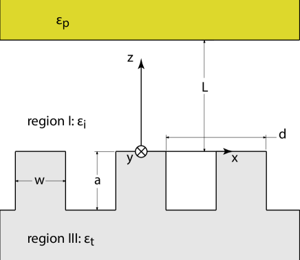
Figure 1: A 1D lamellar grating and its associated reference frame.

For an incident wave characterized by a wave vector $\mathbf{k}_{i}^{(p)}=(\alpha_{p},k_{y},-\gamma_{p}^{(i)})$ a grating structure with period $d$ will generate an infinite number of reflected waves with wave vectors $\mathbf{k}_{r}^{(n)}=(\alpha_{n},k_{y},\gamma_{n}^{(i)})$ and transmitted waves with wave vectors $\mathbf{k}_{t}^{(n)}=(\alpha_{n},k_{y},-\gamma_{n}^{(t)})$. $\alpha_{n}=k_{x}+n\frac{2\pi}{d}$ and $\gamma_{n}^{(i/t)}=\left(\epsilon_{i/t}\omega^{2}-\alpha_{n}^{2}-k_{y}^{2}\right)^{1/2}$.

In region I, the $y$-components of the fields are written as a Rayleigh expansion involving incident and reflected fields of order $p$ and $n$ respectively

$$\begin{split}E_{y}(x,z)&=\sum_{n=-\infty}^{+\infty}\delta_{np}I_{p}^{(e)}e^{\imath(\alpha_{p}x-\gamma_{p}^{(i)}z)}\\ &+R_{np}^{(e)}e^{\imath(\alpha_{n}x+\gamma_{n}^{(i)}z)}\end{split}$$ (2a)

$$\begin{split}H_{y}(x,z)&=\sum_{n=-\infty}^{+\infty}\delta_{np}I_{p}^{(h)}e^{\imath(\alpha_{p}x-\gamma_{p}^{(i)}z)}\\ &+R_{np}^{(h)}e^{\imath(\alpha_{n}x+\gamma_{n}^{(i)}z)}\end{split}$$ (2b)

whereas in region III, the Rayleigh expansion involves the transmitted fields

$$E_{y}(x,z) =\sum_{n=-\infty}^{+\infty}T_{np}^{(e)}e^{\imath(\alpha_{n}x-\gamma_{n}^{(t)}(z+a))}$$ (3a)

$$H_{y}(x,z) =\sum_{n=-\infty}^{+\infty}T_{np}^{(h)}e^{\imath(\alpha_{n}x-\gamma_{n}^{(t)}(z+a))}$$ (3b)

Whether in region I or III, the $x$-components of the fields are obtained from the $y$-components thanks to the Maxwell’s curl equations

$$\begin{split}E_{x}(x,z)&=\frac{\imath k_{y}}{\epsilon_{i/t}\omega^{2}-k_{y}^{2}}\partial_{x}E_{y}(x,z)\\ &+\frac{\imath\omega}{\epsilon_{i/t}\omega^{2}-k_{y}^{2}}\partial_{z}H_{y}(x,z)\end{split}$$ (4a)

$$\begin{split}H_{x}(x,z)&=\frac{\imath k_{y}}{\epsilon_{i/t}\omega^{2}-k_{y}^{2}}\partial_{x}H_{y}(x,z)\\ &-\frac{\imath\omega\epsilon_{i/t}}{\epsilon_{i/t}\omega^{2}-k_{y}^{2}}\partial_{z}E_{y}(x,z)\end{split}$$ (4b)

In the grating region $-a\leq z\leq 0$, owing to the periodicity along the $x$ direction the fields as well as the permittivity $\epsilon(x)$ and its reciprocal $1/\epsilon(x)$ can be expanded in Fourier series. We have

$$E_{x}(x,z) =\sum_{n}e_{x}^{(n)}(z)e^{\imath k_{x}x}e^{2\imath n\pi x/d}$$ (5a)

$$E_{y}(x,z) =\sum_{n}e_{y}^{(n)}(z)e^{\imath k_{x}x}e^{2\imath n\pi x/d}$$ (5b)

$$H_{x}(x,z) =\sum_{n}h_{x}^{(n)}(z)e^{\imath k_{x}x}e^{2\imath n\pi x/d}$$ (5c)

$$H_{y}(x,z) =\sum_{n}h_{y}^{(n)}(z)e^{\imath k_{x}x}e^{2\imath n\pi x/d}$$ (5d)

$$\epsilon(x) =\sum_{n}\epsilon_{n}e^{2\imath n\pi x/d}$$ (5e)

$$1/\epsilon(x) =\sum_{n}\backepsilon_{n}e^{2\imath n\pi x/d}$$ (5f)

With those notations, we are able to express the Maxwell’s curl equations in a compact matrix form. Let $\mathbf{F}$ be a column vector collecting the Fourier components of the fields $\mathbf{F}=(\mathbf{e}_{x},\mathbf{e}_{y},\mathbf{h}_{x},\mathbf{h}_{y})^{\mathsf{T}}$, we may write

$$\partial_{z}\mathbf{F} =\mathbf{M}\mathbf{F}$$ (6a)

$$\mathbf{M} =\begin{pmatrix}\mathbf{0}&\mathbf{0}&-\frac{\imath k_{y}}{\omega}\boldsymbol{\alpha}\boldsymbol{\epsilon}^{-1}&-\imath\omega\mathbf{1}+\frac{\imath}{\omega}\boldsymbol{\alpha}\boldsymbol{\epsilon}^{-1}\boldsymbol{\alpha}\\ \mathbf{0}&\mathbf{0}&\imath\omega\mathbf{1}-\frac{\imath k_{y}^{2}}{\omega}\boldsymbol{\epsilon}^{-1}&\frac{\imath k_{y}}{\omega}\boldsymbol{\epsilon}^{-1}\boldsymbol{\alpha}\\ \frac{\imath k_{y}}{\omega}\boldsymbol{\alpha}&\imath\omega\boldsymbol{\epsilon}-\frac{\imath}{\omega}\boldsymbol{\alpha}\boldsymbol{\alpha}&\mathbf{0}&\mathbf{0}\\ -\imath\omega\boldsymbol{\backepsilon}^{-1}+\frac{\imath k_{y}^{2}}{\omega}\mathbf{1}&-\frac{\imath k_{y}}{\omega}\boldsymbol{\alpha}&\mathbf{0}&\mathbf{0}\end{pmatrix}\equiv\begin{pmatrix}\mathbf{0}&\mathbf{M}_{1}\\ \mathbf{M}_{2}&\mathbf{0}\end{pmatrix}$$ (6b)

In the above equation, $\boldsymbol{\alpha}=\text{diag}(\alpha_{n})$, $\mathbf{1}$ is the identity and $\boldsymbol{\epsilon}$, resp. $\boldsymbol{\backepsilon}$, are Toeplitz matrices whose structure is defined as having elements $\{\epsilon_{n},n\geq 0\}$ on the first line and elements $\{\epsilon_{n},n\leq 0\}$ on the first column. Note that in accordance with ref. Lalanne and Morris (1996), we have replaced the matrix $\boldsymbol{\epsilon}$ by $\boldsymbol{\backepsilon}^{-1}$ in the lower-left block of the matrix $\mathbf{M}$. This constitutes an improvement with respect to ref. Lambrecht and Marachevsky (2008), where this replacement had not been done. The matrix $\mathbf{F}$ has dimension $4\times 1$ in units of $2N+1$. A particular column of $\mathbf{F}$ corresponds to a particular incident order $p$. In the following, bold quantities are matrices whose dimensions will be given in units of $2N+1$ if not trivial. As an example, in eq. (6b) $\boldsymbol{\alpha}$, $\boldsymbol{\epsilon}$, $\boldsymbol{\backepsilon}$ and $\mathbf{1}$ are matrices of dimension $1\times 1$ whereas $\mathbf{M}_{1}$ and $\mathbf{M}_{2}$ are of dimension $2\times 2$.

In Lambrecht and Marachevsky (2008) eqn. (6a) had been numerically solved. Here we follow a different path which has proven to lead to more stable numerical calculations. Because of the block anti-diagonal structure of matrix $\mathbf{M}$, eq. (6a) can be recast as a Helmholtz-like equation for the electric fields provided that $\mathbf{M}$ is independent of $z$ which is the case for the lamellar gratings we consider here

$$\partial^{2}_{z^{2}}\begin{pmatrix}\mathbf{e}_{x}\\ \mathbf{e}_{y}\end{pmatrix}=\mathbf{M}_{1}\mathbf{M}_{2}\begin{pmatrix}\mathbf{e}_{x}\\ \mathbf{e}_{y}\end{pmatrix}\equiv\mathbf{M}^{(e)}\begin{pmatrix}\mathbf{e}_{x}\\ \mathbf{e}_{y}\end{pmatrix}$$ (7)

This equation is solved as $\begin{pmatrix}\mathbf{e}_{x}\\ \mathbf{e}_{y}\end{pmatrix}(z)=e^{\sqrt{\mathbf{M}^{(e)}}z}\mathbf{C^{+}}+e^{-\sqrt{\mathbf{M}^{(e)}}z}\mathbf{C^{-}}$ where $\mathbf{C^{+}}$ and $\mathbf{C^{-}}$ are unknown coefficients to be determined. Let $\boldsymbol{\phi}$, $\boldsymbol{\lambda}$ be respectively the eigenvectors and eigenvalues of the matrix $\mathbf{M}^{(e)}$ such that $\mathbf{M}^{(e)}=\boldsymbol{\phi}\,\text{diag}(\boldsymbol{\lambda})\,\boldsymbol{\phi}^{-1}$. Writing explicitly the expression for $e^{\pm\sqrt{\mathbf{M}^{(e)}}z}$, we can include the matrix $\boldsymbol{\phi}^{-1}$ in the unknown coefficients $\mathbf{C^{+}}$ and $\mathbf{C^{-}}$; furthermore we want to avoid exponentially growing solutions at $z=-a$. Following the prescriptions in Moharam et al. (1995) we finally arrive at

$$\begin{pmatrix}\mathbf{e}_{x}\\ \mathbf{e}_{y}\end{pmatrix}(z) =\boldsymbol{\phi}e^{\sqrt{\boldsymbol{\lambda}}z}\mathbf{C^{+}}+\boldsymbol{\phi}e^{-\sqrt{\boldsymbol{\lambda}}(z+a)}\mathbf{C^{-}}$$ (8a)

$$\begin{split}\begin{pmatrix}\mathbf{h}_{x}\\ \mathbf{h}_{y}\end{pmatrix}(z)&=\mathbf{M}^{-1}_{1}\boldsymbol{\phi}\sqrt{\boldsymbol{\lambda}}e^{\sqrt{\boldsymbol{\lambda}}z}\mathbf{C^{+}}\\ &-\mathbf{M}^{-1}_{1}\boldsymbol{\phi}\sqrt{\boldsymbol{\lambda}}e^{-\sqrt{\boldsymbol{\lambda}}(z+a)}\mathbf{C^{-}}\end{split}$$ (8b)

where eq. (8b) has been obtained by injecting eq. (8a) into $\begin{pmatrix}\mathbf{h}_{x}\\ \mathbf{h}_{y}\end{pmatrix}=\mathbf{M}^{-1}_{1}\partial_{z}\begin{pmatrix}\mathbf{e}_{x}\\ \mathbf{e}_{y}\end{pmatrix}$ from eq. (6b).

We can use eqs. (2) and eqs. (4) to write the fields at $z=0$ and eqs. (3) to write the fields at $z=-a$. In compact matrix form, this leads to

$$\begin{split}\mathbf{F}(-a)&=\begin{pmatrix}-\frac{k_{y}\boldsymbol{\alpha}}{\epsilon_{t}\omega^{2}-k_{y}^{2}}&\frac{\omega\boldsymbol{\gamma}^{(t)}}{\epsilon_{t}\omega^{2}-k_{y}^{2}}\\ \mathbf{1}&\mathbf{0}\\ -\frac{\omega\epsilon_{t}\boldsymbol{\gamma}^{(t)}}{\epsilon_{t}\omega^{2}-k_{y}^{2}}&-\frac{k_{y}\boldsymbol{\alpha}}{\epsilon_{t}\omega^{2}-k_{y}^{2}}&\\ \mathbf{0}&\mathbf{1}\end{pmatrix}\begin{pmatrix}\mathbf{T}^{(e)}\\ \mathbf{T}^{(h)}\end{pmatrix}\\ &\equiv\begin{pmatrix}\mathbf{t}_{e}\\ \mathbf{t}_{h}\end{pmatrix}\begin{pmatrix}\mathbf{T}^{(e)}\\ \mathbf{T}^{(h)}\end{pmatrix}\end{split}$$ (9)

and

$$\begin{split}\mathbf{F}(0)&=\begin{pmatrix}-\frac{k_{y}\boldsymbol{\alpha}}{\epsilon_{i}\omega^{2}-k_{y}^{2}}&\frac{\omega\boldsymbol{\gamma}^{(i)}}{\epsilon_{i}\omega^{2}-k_{y}^{2}}\\ \mathbf{1}&\mathbf{0}\\ -\frac{\omega\epsilon_{i}\boldsymbol{\gamma}^{(i)}}{\epsilon_{i}\omega^{2}-k_{y}^{2}}&-\frac{k_{y}\boldsymbol{\alpha}}{\epsilon_{i}\omega^{2}-k_{y}^{2}}\\ \mathbf{0}&\mathbf{1}\end{pmatrix}\begin{pmatrix}\mathbf{I}^{\sigma=e}\\ \mathbf{I}^{\sigma=h}\end{pmatrix}\\ &+\begin{pmatrix}-\frac{k_{y}\boldsymbol{\alpha}}{\epsilon_{i}\omega^{2}-k_{y}^{2}}&-\frac{\omega\boldsymbol{\gamma}^{(i)}}{\epsilon_{i}\omega^{2}-k_{y}^{2}}\\ \mathbf{1}&\mathbf{0}\\ \frac{\omega\epsilon_{i}\boldsymbol{\gamma}^{(i)}}{\epsilon_{i}\omega^{2}-k_{y}^{2}}&-\frac{k_{y}\boldsymbol{\alpha}}{\epsilon_{i}\omega^{2}-k_{y}^{2}}&\\ \mathbf{0}&\mathbf{1}\end{pmatrix}\begin{pmatrix}\mathbf{R}^{(e)}\\ \mathbf{R}^{(h)}\end{pmatrix}\\ &\equiv\begin{pmatrix}\mathbf{i}_{ee}&\mathbf{i}_{eh}\\ \mathbf{i}_{he}&\mathbf{i}_{hh}\end{pmatrix}\begin{pmatrix}\mathbf{I}^{\sigma=e}\\ \mathbf{I}^{\sigma=h}\end{pmatrix}+\begin{pmatrix}\mathbf{r}_{e}\\ \mathbf{r}_{h}\end{pmatrix}\begin{pmatrix}\mathbf{R}^{(e)}\\ \mathbf{R}^{(h)}\end{pmatrix}\end{split}$$ (10)

where $\boldsymbol{\gamma}^{(i/t)}=\text{diag}(\gamma_{n}^{(i/t)})$ and we have introduced the basis of polarizations $\sigma$ we use, denoted $e$ and $h$. The polarizations $\sigma=e,h$ are defined by imposing $H_{y}=0$ and $E_{y}=0$ respectively. Hence, in the above equation for incident $\sigma=e$ waves, we impose $\mathbf{I}^{\sigma=e}=\mathbf{1}$ and $\mathbf{I}^{\sigma=h}=\mathbf{0}$ and vice-versa for incident $\sigma=h$ waves. Note that $\mathbf{t}_{e}$, $\mathbf{t}_{h}$, $\mathbf{r}_{e}$ and $\mathbf{r}_{h}$ are of dimension $2\times 2$ whereas $\mathbf{i}_{ee}$, $\mathbf{i}_{eh}$, $\mathbf{i}_{he}$ and $\mathbf{i}_{hh}$ are of dimension $2\times 1$. Other dimensions are deduced so as to be consistent with those of $\mathbf{F}$.

Evaluating eqs. (8) at $z=-a$ and $z=0$ and identifying with eqs. (9) and  (10) leads to a linear system of equations of dimension $8(2N+1)$ for the $8(2N+1)$ unknowns $\mathbf{C^{+}}$, $\mathbf{C^{-}}$, $\mathbf{R}^{(e)}$, $\mathbf{R}^{(h)}$, $\mathbf{T}^{(e)}$ and $\mathbf{T}^{(h)}$. Nevertheless, it is numerically more stable to eliminate the reflection and transmission unknowns from this system and to solve instead a reduced system of dimension $4(2N+1)$ for solely $\mathbf{C^{+}}$ and $\mathbf{C^{-}}$. All done, this system reads:

$$\begin{pmatrix}\left(\boldsymbol{\phi}-\mathbf{t}_{e}\mathbf{t}^{-1}_{h}\mathbf{V}\right)e^{-\sqrt{\boldsymbol{\lambda}}a}&\boldsymbol{\phi}+\mathbf{t}_{e}\mathbf{t}^{-1}_{h}\mathbf{V}\\ \boldsymbol{\phi}-\mathbf{r}_{e}\mathbf{r}^{-1}_{h}\mathbf{V}&\left(\boldsymbol{\phi}+\mathbf{r}_{e}\mathbf{r}^{-1}_{h}\mathbf{V}\right)e^{-\sqrt{\boldsymbol{\lambda}}a}\end{pmatrix}\begin{pmatrix}\mathbf{C^{+}}\\ \mathbf{C^{-}}\end{pmatrix}=\begin{pmatrix}\mathbf{0}\\ \begin{pmatrix}\mathbf{i}_{ee}-\mathbf{r}_{e}\mathbf{r}^{-1}_{h}\mathbf{i}_{he}&\mathbf{i}_{eh}-\mathbf{r}_{e}\mathbf{r}^{-1}_{h}\mathbf{i}_{hh}\end{pmatrix}\begin{pmatrix}\mathbf{I}^{\sigma=e}\\ \mathbf{I}^{\sigma=h}\end{pmatrix}\end{pmatrix}$$ (11)

where we have defined $\mathbf{V}=\mathbf{M}^{-1}_{1}\boldsymbol{\phi}\sqrt{\boldsymbol{\lambda}}$. Once the unknown coefficients $\mathbf{C^{+}}$ and $\mathbf{C^{-}}$ are determined by solving eq. (11), the reflection and transmission coefficients are:

$$\begin{pmatrix}\mathbf{R}^{(e)}\\ \mathbf{R}^{(h)}\end{pmatrix} =\mathbf{r}^{-1}_{h}\left(\mathbf{V}\left(\mathbf{C^{+}}-e^{-\sqrt{\boldsymbol{\lambda}}a}\mathbf{C^{-}}\right)\right.$$ (12a)

$$\left.-\begin{pmatrix}\mathbf{i}_{he}&\mathbf{i}_{hh}\end{pmatrix}\begin{pmatrix}\mathbf{I}^{\sigma=e}\\ \mathbf{I}^{\sigma=h}\end{pmatrix}\right)$$

$$\begin{pmatrix}\mathbf{T}^{(e)}\\ \mathbf{T}^{(h)}\end{pmatrix} =\mathbf{t}^{-1}_{h}\left(\mathbf{V}\left(e^{-\sqrt{\boldsymbol{\lambda}}a}\mathbf{C^{+}}-\mathbf{C^{-}}\right)\right)$$ (12b)

Resolution of eq. (11) and eqs. (12) first for incident $\sigma=e$ waves and then for incident $\sigma=h$ waves leads to the complete reflection and transmission matrices $\mathbf{R}_{g}$ and $\mathbf{T}_{g}$:

$$\mathbf{R}_{g} =\begin{pmatrix}\mathbf{R}^{(e)}(\sigma=e)&\mathbf{R}^{(e)}(\sigma=h)\\ \mathbf{R}^{(h)}(\sigma=e)&\mathbf{R}^{(h)}(\sigma=h)\end{pmatrix}$$ (13a)

$$\mathbf{T}_{g} =\begin{pmatrix}\mathbf{T}^{(e)}(\sigma=e)&\mathbf{T}^{(e)}(\sigma=h)\\ \mathbf{T}^{(h)}(\sigma=e)&\mathbf{T}^{(h)}(\sigma=h)\end{pmatrix}$$ (13b)

The force at $T=0$ K is recovered by the substitution:

$$2\pi k_{B}T\sum_{n=0}^{\infty}{}^{{}^{\prime}}\to\hbar\int_{0}^{\infty}\mathrm{d}\xi$$ (14)

We define two quantities, $\vartheta_{F}(L)$ and $\eta_{F}(L)$ to assess respectively the effect of the finite temperature and the deviation from PFA:

$$\vartheta_{F}(L) =\frac{F_{p,g}(L;T=300\,K)}{F_{p,g}(L;T=0\,K)}$$ (15)

$$\eta_{F}(L;T) =\frac{F_{p,g}(L;T)}{F^{PFA}_{p,g}(L;T)}$$ (16)

where $F^{PFA}_{p,g}(L;T)=\frac{1}{d}\int_{0}^{d}F_{p,p}(L(x);T)\text{d}x$ and $F_{p,p}(L;T)$ the force between two plane-parallel plates is given by the Lifshitz formula Lifshitz (1956).

.0.3 Numerical evaluations

We now study the thermal Casimir interaction between a gold plate and a doped silicon grating. Therefore, $\epsilon_{t}\equiv\epsilon_{Si}(\omega)$ and $\epsilon_{p}\equiv\epsilon_{Au}(\omega)$. The plate and the grating are separated by vacuum $\epsilon_{i}\equiv\epsilon_{0}=1$ $\forall\omega$. As described in Bao et al. (2010), the permittivity of gold is taken from experimental data extrapolated to low frequencies by the Drude model. The permittivity of doped silicon is modeled by a two-oscillator model: one describing the intrinsic part of silicon and the other one describing its metallic behavior at low frequencies Lambrecht et al. (2007). The metallic part of doped silicon is determined by a doping level of $2\times 10^{18}$ cm^-3. The situation is characterized by four length scales: the separation distance $L$, the corrugation height $a$, the grating period $d$ and the corrugation width $w$ (for this last quantity, we will prefer to work with the filling factor $f=w/d$). A complete analysis would in principle involve full Casimir force calculations in a four dimensional parameters space. Instead we explore here the parameter space at fixed filling factor and grating period $d$ corresponding to the experimental set-up in Bao et al. (2010).

In figure 2

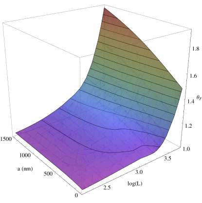
Figure 2: Effect of temperature on the Casimir force given by the ratio $\vartheta_{F}$ as a function of the separation distance $L$ and corrugation depth $a$.

we illustrate the effect of the temperature in the plate-grating geometry by plotting the ratio $\vartheta_{F}(L,a)$ as a function of both the separation distance $L$ and the trench depth $a$. The grating period $d$ and the filling factor $f$ are fixed respectively at $d=400$ nm and $f=0.5$. For this choice of materials, we find over the whole range of parameters $\vartheta_{F}(L,a)>1$ so that the thermal photons always lead to an increase in the Casimir force. For $a=0$ we recover the two-plate configuration and we have necessarily $\lim_{L\to 0}\vartheta_{F}(L,a=0)=1$. The total temperature effect $\vartheta_{F}(L,a=\infty)-\vartheta_{F}(L,a=0)$ increases with larger separation distances $L$. The limiting value $\vartheta_{F}(L,a=\infty)$ is reached for larger $a$ as the separation distance $L$ increases since this limiting value rather means $a>>L$.

Interestingly, for a fixed separation distance $L$, there is a steep increase of $\vartheta_{F}$ as a function of the corrugation depth $a$ towards saturation as shown in detail in figure 3.

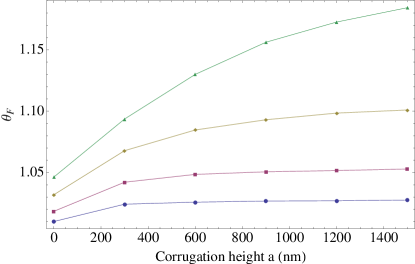
Figure 3: Effect of the temperature $\vartheta_{F}$ on the Casimir force for $L$=150, 300, 600, 1200 nm (from bottom to top) as a function of the trench depth $a$.

At a distance of $1.2\mu$m the temperature corrections increase the zero temperature force by $\sim 5\%$ between two flat plates. Remarkably, this increase becomes $\sim 20\%$ if the doped Si plate contains deep trenches ($a\sim 1.4\mu$m). For $L=600$ nm the effect is less pronounced but still amounts to an increase from 3% to about 10%. Clearly the use of a structured surface increases the thermal Casimir force and makes the effect easier to be observed at shorter distances. A possible explanation is that the nanostructures change the spectral mode density especially in the infrared frequency domain, so that thermal effects become enhanced, as it has already been pointed out in heat transfer phenomena between gratings Guérout et al. (2012); Lussange et al. (2012).

Next, we turn to assess the validity of PFA. Figure 4

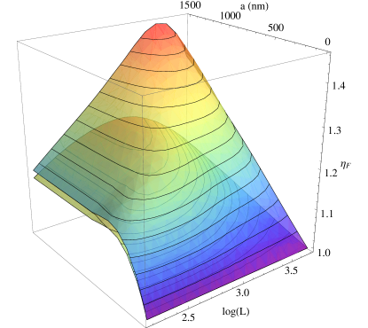
Figure 4: Deviation from PFA $\eta_{F}$ as a function of the separation distance $L$ and trench depth $a$. The lower surface is for $T=0$ K, the upper one for $T=300$ K.

shows the deviation from PFA $\eta_{F}$ as a function of the separation distance $L$ and the corrugation depth $a$. By definition $\eta_{F}(L,a=0)=1$. For a fixed separation distance $L$, the error made by PFA increases with deeper trench depth $a$. We have $\eta_{F}(L,a;T=300\,K)>\eta_{F}(L,a;T=0\,K)$ for all values of separation distance $L$ and trench depth $a$ so that a finite temperature is seen to always increase the deviation from PFA. At large separation distances, we expect PFA to be valid so that $\lim_{L\to\infty}\eta_{F}(L,a;T)=1$. In particular, for a fixed corrugation depth $a$, the functions $\eta_{F}$ show a maximum for a particular distance $L=L_{\mathrm{max}}$ as illustrated in figure 5.

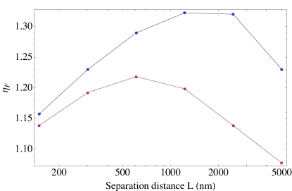
Figure 5: Deviation from PFA $\eta_{F}$ at fixed trench depth $a=900$ nm as a function of the separation distance $L$ for $T=0$ K (bottom) and $T=300$ K (top).

Qualitatively, we can say that this value $L_{\mathrm{max}}\approx a$. More precisely we find $L_{max}\lessapprox a$ for $T=0$ K and $L_{max}\gtrapprox a$ for $T=300$ K. Thus the deviation from PFA increases with increasing distances for $L\leq a$ and decreases with increasing distances for $L\geq a$. The deviation from PFA for $T\neq 0$ K shows the same qualitative behavior as for $T=0$ K.

.0.4 Comparison with experimental data

We are now in the position to compare our calculations with experimental data from Chan et al. (2008); Bao et al. (2010). In these experiments the interaction between a nanostructured silicon surface and a gold-coated sphere with a radius of 50 $\mu$m was measured. The force was detected at ambient temperature using a silicon micromechanical resonator onto which the gold sphere was attached. As the distance between the nanostructured surface and the sphere was varied, the change in the resonant frequency of the resonator was recorded. This quantity is proportional to the Casimir force gradient $\partial_{L}F_{s,g}(L)$ between the gold sphere and the silicon grating. Since the separation distance between the sphere and the grating is small compared to the radius of the sphere, we can relate this Casimir force gradient to the Casimir pressure $F_{p,g}(L)$ between a plate and the grating as $\partial_{L}F_{s,g}(L)=2\pi RF_{p,g}(L)$. Under these assumptions, the measured quantity $\partial_{L}F_{s,g}(L)$ when normalized by its PFA value is identical to $\eta_{F}$, i.e. $\partial_{L}F(L)/\partial_{L}F^{PFA}(L)=\eta_{F}(L)$ where we have omitted for simplicity the indices indicating the sphere grating geometry.

In figure 6

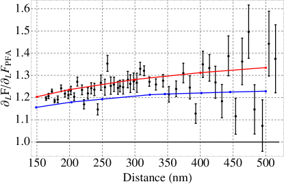
Figure 6: Experimental data for the Casimir force gradient between a gold sphere and a silicon grating with deep trenches (black dots with error bars). The data are normalized to their PFA expression. This is compared with our calculations both for $T=0$ K (blue) and $T=300$ K (red).

we plot $\eta_{F}(L)$ for a silicon structure with deep trenches (sample B in Ref. Chan et al. (2008)). This sample has a period $d=400$ nm, trench depth $a=980$ nm and filling factor $f=0.478$. The experimental data are plotted as circles with error bars. Our calculations for $T=0$ K and $T=300$ K are plotted as the blue and red curves respectively. As first reported in Chan et al. (2008), the measured values of $\eta_{F}(L)$ between gold and silicon surfaces were found to be smaller than predictions using perfect reflectors at zero temperature Büscher and Emig (2004). The inclusion of the material properties at zero temperature leads to better agreement Lambrecht and Marachevsky (2008). Our zero-temperature results presented here are larger than those in Lambrecht and Marachevsky (2008) by about $\partial_{L}F/\partial_{L}F^{PFA}\approx 0.05$. We attribute this difference to the replacement of the matrix $\boldsymbol{\epsilon}$ by $\boldsymbol{\backepsilon}^{-1}$ in the lower-left block of the matrix $\mathbf{M}$ in Eq. (6b) and to solving the differential equations (7) instead of (6a).

Let us now discuss the thermal effects. The red line in figure 6 plots the calculated results for $T=300$ K, at separation $L$ from $\approx 150$ nm to $L\approx 500$ nm. Following our previous discussion of Fig. (5), since the experiment was conducted in a regime where $L<a$, both $\eta_{F}$ and $\partial_{L}F/\partial_{L}F^{PFA}$ increase with separation distance. In figure 6, the difference between the red line for $T=300$ K and the blue line for $T=0$ K is clearly visible. When compared to the experimental data measured at ambient temperature, the theory curve calculated for $T=300$ K gives better agreement than the one at $T=0$ K. Unambiguous demonstration of the thermal contributions of the Casimir force in this sample, however, would require experimental improvements to further reduce the measurement uncertainty.

So far, the thermal contributions to the Casimir force has only been observed at distances larger than $1\mu$m between smooth surfaces Sushkov et al. (2012). At smaller distances, the thermal effects decrease significantly. As shown in figure 3, the thermal contributions to the Casimir force between flat surfaces are expected to be only about $3\%$ at $\sim 500$ nm. By replacing one of the surfaces with a grating with deep trenches, the thermal contributions increase by a factor of 3. Nanostructured surfaces therefore hold promise for precise measurements of the thermal Casimir force.

Next, we focus on gratings with shallow trenches that were used in Bao et al. (2010). The period was again $d=400$ nm, but the trench depth was only $a=98$ nm. The filling factor was approximately $f=0.48$. Figure 7 shows the measured data points from this experiment together with the results of our calculations for this sample both at $T=300$ K (red curve) and $T=0$ K (blue curve). In the calculation we take into account the exact trapezoidal shape of the corrugation profile via a generalization of the formalism presented above Lussange et al. (2012). As the range of separation distances is the same as in the experiment with deep trenches the situation now corresponds to a regime where $L>a$. Therefore $\eta_{F}$ and thus $\partial_{L}F/\partial_{L}F^{PFA}$ both decrease with increasing distance to reach its asymptotic value of 1. Again the theoretical prediction at 300K is in good agreement with the measured data. The overall temperature effect is less pronounced here than for the deep trenches as the trench depth is about a factor of 10 smaller.

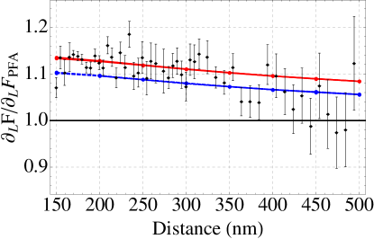
Figure 7: Experimental data for the Casimir force gradient between a gold sphere and a silicon grating with shallow trenches (black dots with error bars). The data are normalized to their PFA expression. This is compared with our calculations both for $T=0$ K (blue) and $T=300$ K (red).

.0.5 Conclusions

We have calculated the Casimir interaction between a plate and a grating at finite temperature. We find good agreement between our calculations for $T=300$ K and experimental data taken at ambient temperature. Even though the experiments are performed at relatively small separation distances $L<500$ nm, the use of gratings enhances the thermal contributions of the Casimir force. Our findings provide an alternative approach to study thermal Casimir forces without having to reach separation distances of the order of microns.

H.B.C. is supported by HKUST 600511 from the Research Grants Council of Hong Kong SAR, Shun Hing Solid State Clusters Lab and DOE Grant No. DE-FG02-05ER46247.

We thank the European Science Foundation (ESF) within the activity New Trends and Applications of the Casimir Effect (www.casimir-network.com) for support.

References

- Casimir (1948) H. Casimir, Proc. Kon. Ned. Ak. Wet, 51, 793 (1948).
- Mehra (1967) J. Mehra, Physica, 37, 145 (1967), ISSN 0031-8914.
- Sushkov et al. (2012) A. Sushkov, W. Kim, D. Dalvit, and S. Lamoreaux, Nat. Phys., 7, 230 (2012).
- Büscher and Emig (2004) R. Büscher and T. Emig, Phys. Rev. A, 69, 062101 (2004).
- Lambrecht and Marachevsky (2008) A. Lambrecht and V. N. Marachevsky, Phys. Rev. Lett., 101, 160403 (2008).
- Davids et al. (2010) P. S. Davids, F. Intravaia, F. S. S. Rosa, and D. A. R. Dalvit, Phys. Rev. A, 82, 062111 (2010).
- M.T. Jaekel and S. Reynaud (1991) M.T. Jaekel and S. Reynaud, J. Phys. I France, 1, 1395 (1991).
- Lambrecht et al. (2006) A. Lambrecht, P. A. M. Neto, and S. Reynaud, New J. Phys., 8, 243 (2006).
- Emig et al. (2007) T. Emig, N. Graham, R. L. Jaffe, and M. Kardar, Phys. Rev. Lett., 99, 170403 (2007).
- Chan et al. (2008) H. B. Chan, Y. Bao, J. Zou, R. A. Cirelli, F. Klemens, W. M. Mansfield, and C. S. Pai, Phys. Rev. Lett., 101, 030401 (2008).
- Bao et al. (2010) Y. Bao, R. Guérout, J. Lussange, A. Lambrecht, R. A. Cirelli, F. Klemens, W. M. Mansfield, C. S. Pai, and H. B. Chan, Phys. Rev. Lett., 105, 250402 (2010).
- Moharam et al. (1995) M. G. Moharam, D. A. Pommet, E. B. Grann, and T. K. Gaylord, J. Opt. Soc. Am. A, 12, 1077 (1995).
- Lalanne and Morris (1996) P. Lalanne and G. M. Morris, J. Opt. Soc. Am. A, 13, 779 (1996).
- Lifshitz (1956) E. Lifshitz, Sov. Phys. JETP, 2, 73 (1956).
- Lambrecht et al. (2007) A. Lambrecht, I. Pirozhenko, L. Duraffourg, and P. Andreucci, Eur. Phys. Lett., 77, 44006 (2007).
- Guérout et al. (2012) R. Guérout, J. Lussange, F. F.S.S. Rosa, J.-P. Hugonin, D. Dalvit, J.-J. Greffet, A. Lambrecht, and S. Reynaud, Phys. Rev. B, 85(R), 180301 (2012).
- Lussange et al. (2012) J. Lussange, R. Guérout, F. Rosa, J.-J. Greffet, A. Lambrecht, and S. Reynaud, Phys. Rev. B, 86, 085432 (2012a).
- Lussange et al. (2012) J. Lussange, R. Guérout, and A. Lambrecht, Phys. Rev. A, 86, 062502 (2012b).