Macroscopic optical response and photonic bands

Abstract

We develop a formalism for the calculation of the macroscopic dielectric response of composite systems made of particles of one material embedded periodically within a matrix of another material, each of which is characterized by a well defined dielectric function. The nature of these dielectric functions is arbitrary, and could correspond to dielectric or conducting, transparent or opaque, absorptive and dispersive materials. The geometry of the particles and the Bravais lattice of the composite are also arbitrary. Our formalism goes beyond the longwavelenght approximation as it fully incorporates retardation effects. We test our formalism through the study the propagation of electromagnetic waves in 2D photonic crystals made of periodic arrays of cylindrical holes in a dispersionless dielectric host. Our macroscopic theory yields a spatially dispersive macroscopic response which allows the calculation of the full photonic band structure of the system, as well as the characterization of its normal modes, upon substitution into the macroscopic field equations. We account approximately for the spatial dispersion through a local magnetic permeability and we analyze the resulting dispersion relation, obtaining a region of left-handedness.

1 Introduction

The propagation of light within homogeneous materials is completely characterized by their electromagnetic response. In the optical regime, magnetic effects are typically negligible so that knowledge of the dielectric response is sufficient for the study of wave propagation [1]. However, when the system has spatial inhomogeneities, the behaviour of light is not trivial and has captured the attention of many researchers [2, 3, 4, 5, 6, 7, 8, 9, 10, 11]. The possibility of controlling the propagation of photons by producing artificially structured materials has been widely demonstrated in recent years. Novel effects have been obtained, such as negative refraction, inverse Doppler effect, optical invisibility cloaking, optical magnetism etc. [12, 13, 14, 15].

Effective medium theories [16, 17, 18, 19, 20, 21, 22, 23, 24] have been proposed to describe inhomogeneous systems, such as diluted colloidal suspensions in the quasistatic or long wavelength limit, in terms of a homogeneous macroscopic response. Further developments in homogenization of composites have been proposed [25, 26, 27, 28, 29, 30, 31, 32, 33] and their limits of validity have have been discussed [2, 34, 35].

In this paper we obtain the macroscopic optical response using a computationally efficient reformulation of a procedure [5, 6] original developed to account for the local field effect of systems with spatial fluctuations. Our main result is that for any system, the macroscopic response to an external excitation is simply the average projection of the corresponding microscopic response. We apply this general result to Maxwell equations in order to obtain an explicit expression for the macroscopic dielectric response of binary composites. We illustrate its use with numerical results for a 2D periodic photonic crystal. As the wavelength of the electromagnetic field becomes comparable to the characteristic microscopic spatial lengthscale of the system, the macroscopic response becomes highly non-local, with a strong dependence on the wavevector besides its usual dependence on frequency. When the full spatial dispersion is taken into account, the photonic band structure of the system can be obtained and analyzed from its macroscopic response.

The paper is organized as follows: In Sec. 2 we formulate a general theory for the macroscopic dielectric response of composite systems. In Sec. 3 we adapt our formulation to periodic systems made of two alternating materials, each characterized by well defined dielectric functions. In Sec. 4 we develop an efficient computational scheme which allows the numerical calculation of the macroscopic response without recourse to explicit operations between large matrices. In Sec. 5 we obtain the non-local macroscopic dielectric tensor and use it to calculate macroscopically the full band structure of a 2D photonic crystal made up of non-dispersive dielectric components; we compare it to exact results as well as to results within a local approximation that partially accounts for spatial dispersion through an effective magnetic permeability. Finally, in Sec. 6 we present our conclusions.

2 General theory

Consider a non-magnetic inhomogeneous system characterized by its dielectric response $\hat{\epsilon}$, defined through the constitutive equation $\mathbf{D}=\hat{\epsilon}\mathbf{E}$, where $\mathbf{D}$ and $\mathbf{E}$ are the microscopic displacement and electric fields respectively. We designate these fields as microscopic as they have spatial fluctuations due to the inhomogeneities of the material. They are not microscopic in the atomic scale, but rather, on the scale of the spatial inhomogeneities of the system. We use a caret ($\,\hat{}\,$) over a symbol to denote its operator nature and we leave implicit the dependence of the dielectric response on position as well as on frequency. Our purpose is to obtain the macroscopic dielectric response of the system, relating the macroscopic displacement and electric fields, from which the fluctuations have been removed.

We start from Maxwell equations for monochromatic microscopic fields. We follow the usual procedure [36] to decouple the magnetic field from the electric field to obtain the second order wave equation

$${\hat{\mathcal{W}}}\mathbf{E}=\frac{4\pi c}{iq}\mathbf{J}$$ (1)

where

$${{\hat{\mathcal{W}}}}=\hat{\epsilon}-\frac{1}{q^{2}}\nabla\times\nabla\times=\hat{\epsilon}+\frac{1}{q^{2}}\nabla^{2}{\hat{\mathcal{P}}}^{T}$$ (2)

is the wave operator, $q=\omega/c$ is the wavenumber of light in vacuum, $\omega$ is the frequency, $c$ is the speed of light in vacuum and $\mathbf{J}$ is the external electric current density. Here we introduced the transverse projector ${\hat{\mathcal{P}}}^{T}$ such that the transverse projection of a field $\mathbf{F}$ is $\mathbf{F}^{T}={\hat{\mathcal{P}}}^{T}\mathbf{F}$. For completeness, we also introduce the longitudinal projector ${\hat{\mathcal{P}}}^{L}$ such that ${\hat{\mathcal{P}}}^{L}+{\hat{\mathcal{P}}}^{T}=\hat{1}$, with $\hat{1}$ the identity operator. Notice that Eq. (1) contains both a longitudinal and a transverse part, so it describes not only transverse waves, but also allows for the possible excitation of longitudinal waves such as plasmons [37].

We solve Eq. (1) formally for $\mathbf{E}$ to obtain

$$\mathbf{E}=\frac{4\pi c}{iq}{{\hat{\mathcal{W}}}}^{-1}\mathbf{J}.$$ (3)

As we are interested on the macroscopic response of the system, we introduce the average ${\hat{\mathcal{P}}}_{a}$ and fluctuation ${\hat{\mathcal{P}}}_{f}$ projectors, such that an arbitrary field $\mathbf{F}$ can be written as $\mathbf{F}=\mathbf{F}_{a}+\mathbf{F}_{f}$ with $\mathbf{F}_{a}={\hat{\mathcal{P}}}_{a}\mathbf{F}$ its average and $\mathbf{F}_{f}={\hat{\mathcal{P}}}_{f}\mathbf{F}$ its fluctuating part, and we identify the average field with the macroscopic field $\mathbf{F}_{a}\equiv\mathbf{F}_{M}$. Later, we will provide appropriate explicit definitions for ${\hat{\mathcal{P}}}_{a}$ and ${\hat{\mathcal{P}}}_{f}$; here we remark that they must be idempotent ${\hat{\mathcal{P}}}_{a}^{2}={\hat{\mathcal{P}}}_{a}$, ${\hat{\mathcal{P}}}_{f}^{2}={\hat{\mathcal{P}}}_{f}$, i.e., the average of the average is the average, and the fluctuations of the fluctuations are the fluctuations [5]. Furthermore, ${\hat{\mathcal{P}}}_{a}{\hat{\mathcal{P}}}_{f}={\hat{\mathcal{P}}}_{f}{\hat{\mathcal{P}}}_{a}=0$ and ${\hat{\mathcal{P}}}_{a}+{\hat{\mathcal{P}}}_{f}=\hat{1}$.

As the macroscopic response would be useless unless the external excitations are devoid of microscopic spatial fluctuations, we assume that the external current has no fluctuations, so $\mathbf{J}_{f}=\mathbf{0}$ and $\mathbf{J}=\mathbf{J}^{M}={\hat{\mathcal{P}}}_{a}\mathbf{J}^{M}$, where we used the idempotency of ${\hat{\mathcal{P}}}_{a}$. Thus, acting on both sides of Eq. (3) with ${\hat{\mathcal{P}}}_{a}$ we obtain

$$\mathbf{E}^{M}=\frac{4\pi c}{iq}{\hat{\mathcal{W}}}^{-1}_{aa}\mathbf{J}^{M}.$$ (4)

Here we define ${\hat{\mathcal{O}}}_{\alpha\beta}\equiv{\hat{\mathcal{P}}}_{\alpha}{\hat{\mathcal{O}}}{\hat{\mathcal{P}}}_{\beta}$, with $\alpha,\beta=a,f$ for any operator ${\hat{\mathcal{O}}}$. As Eq. (4) relates the macroscopic external electric current to the macroscopic electric field we may identify the macroscopic inverse wave operator ${\hat{\mathcal{W}}}_{M}^{-1}$,

$$\mathbf{E}^{M}=\frac{4\pi c}{iq}{\hat{\mathcal{W}}}^{-1}_{M}\mathbf{J}^{M}$$ (5)

where

$${\hat{\mathcal{W}}}^{-1}_{M}={\hat{\mathcal{W}}}^{-1}_{aa}.$$ (6)

We summarize this results stating that the macroscopic inverse wave operator is simply the average of the microscopic inverse wave operator. This is a particular case of a more general result: the macroscopic response to an external excitation is simply the average of the corresponding microscopic response.

From the macroscopic Maxwell equations we may further relate the macroscopic wave operator in Eqs. (5) and (6) to the macroscopic dielectric response of the system $\hat{\epsilon}^{M}$ through

$${\hat{\mathcal{W}}}^{M}=\hat{\epsilon}^{M}+\frac{1}{q^{2}}\nabla^{2}{\hat{\mathcal{P}}}_{a}{\hat{\mathcal{P}}}^{T},$$ (7)

in analogy to Eq. (2). Thus, we have to invert the wave operator, average it, and invert it again to finally identify the macroscopic dielectric response. Notice that we have made no approximation whatsoever. We remark that as $\hat{\epsilon}$ relates two fields, $\mathbf{E}$ and $\mathbf{D}$, that have spatial fluctuations, we may not simply average $\hat{\epsilon}$ to obtain its macroscopic counterpart, i.e. $\hat{\epsilon}^{M}\neq\hat{\epsilon}_{aa}$. The difference constitutes the local field effect [5].

Our result may easily be generalizable to other situations and other response functions. The procedure consists on first identifying the response (in our case ${\hat{\mathcal{W}}}^{-1}$) to the external perturbation (i.e. $\mathbf{J}$), and then averaging it to yield the corresponding macroscopic response (i.e. ${\hat{\mathcal{W}}}^{-1}_{M}={\hat{\mathcal{W}}}^{-1}_{aa}$), which may further be related to the desired macroscopic response operator (i.e. $\hat{\epsilon}^{M}$).

3 Periodic binary systems

In this section we use Eq. (6) to obtain the optical properties of an artificial binary crystal made of two materials $A$ and $B$ with dielectric functions $\epsilon_{A}$ and $\epsilon_{B}$. We assume that both media are local and isotropic so that $\epsilon_{A}$ and $\epsilon_{B}$ are simply complex functions of the frequency. For convenience, we will further assume that $\epsilon_{A}$ is real, though this assumption is easily relaxed [38].

We introduce the characteristic function $B(\mathbf{r})$ of the inclusions, such that $B(\mathbf{r})\equiv 1$ whenever $\mathbf{r}$ is on the region $B$ occupied by the inclusions, and $B(\mathbf{r})\equiv 0$ otherwise. Thus, we may write the microscopic dielectric response as

$$\epsilon(\mathbf{r})=\frac{\epsilon_{A}}{u}\left(u-B(\mathbf{r})\right),$$ (8)

where we defined the spectral variable $u\equiv 1/(1-\epsilon_{B}/\epsilon_{A})$ [17]. The microscopic wave operator of Eq. (2) may be written as

$${\hat{\mathcal{W}}}=\frac{\epsilon_{A}}{u}\left(u\hat{g}^{-1}-{\hat{\mathcal{B}}}\right),$$ (9)

where the characteristic operator ${\hat{\mathcal{B}}}$ corresponds to multiplication by $B(\mathbf{r})$ in real space, and we defined

$$\hat{g}=\left(1+\frac{\nabla^{2}{\hat{\mathcal{P}}}^{T}}{q^{2}\epsilon_{A}}\right)^{-1}.$$ (10)

which, as shown below, plays the role of a metric.

Using Eq. (9) we write Eq. (6) as

$${\hat{\mathcal{W}}}^{-1}_{M}=\frac{u}{\epsilon_{A}}\hat{g}_{aa}\left(u-{\hat{\mathcal{B}}}\hat{g}\right)^{-1}_{aa},$$ (11)

where we have taken advantage of the fact that $\hat{g}$ is unrelated to the texture of the crystal, so that it does not couple average to fluctuating fields.

Using Bloch’s theorem [39], we consider an electric field of the form [19]

$$\mathbf{E}_{\mathbf{k}}(\mathbf{r})=\sum_{\mathbf{G}}\mathbf{E}_{\mathbf{G}}e^{i(\mathbf{k}+\mathbf{G})\cdot\mathbf{r}},$$ (12)

where $\mathbf{k}$ is a given wavevector, $\{\mathbf{G}\}$ is the reciprocal lattice of our crystal and the coefficients $\mathbf{E}_{\mathbf{G}}$ represent the field in reciprocal space. In this representation, all operators may be written as matrices with vector index pairs $\mathbf{G},\mathbf{G}^{\prime}$, besides other possible indices, such as Cartesian ones. Thus, we represent the longitudinal projector as the matrix

$$\mathcal{P}^{L}_{\mathbf{G}\mathbf{G}^{\prime}}=\delta_{\mathbf{G}\mathbf{G}^{\prime}}\frac{(\mathbf{k}+\mathbf{G})}{|\mathbf{k}+\mathbf{G}|}\frac{(\mathbf{k}+\mathbf{G}^{\prime})}{|\mathbf{k}+\mathbf{G}^{\prime}|}$$ (13)

with $\delta_{\mathbf{G}\mathbf{G}^{\prime}}$ the Kronecker’s delta, so the transverse projector becomes $\mathcal{P}^{T}_{\mathbf{G}\mathbf{G}^{\prime}}=\mathbf{1}\delta_{\mathbf{G}\mathbf{G}^{\prime}}-\mathcal{P}^{L}_{\mathbf{G}\mathbf{G}^{\prime}}$ with $\mathbf{1}$ the Cartesian identity matrix. The Laplacian operator in reciprocal space is represented by

$$\nabla^{2}\to-(\mathbf{k}+\mathbf{G})^{2}\delta_{\mathbf{G}\mathbf{G}^{\prime}},$$ (14)

and we can define the average projector as a cutoff in the reciprocal space [6]

$$(\mathcal{P}_{a})_{\mathbf{G}\mathbf{G}^{\prime}}=\delta_{\mathbf{G}\mathbf{0}}\delta_{\mathbf{G}^{\prime}\mathbf{0}},$$ (15)

so that average fields simply keep the contributions with vector $\mathbf{k}$ while all other wavevectors are filtered out.

As shown by Eq. (11), we only require

$$(u-{\hat{\mathcal{B}}}\hat{g})^{-1}_{aa}=(u-{\hat{\mathcal{B}}}\hat{g})^{-1}_{\mathbf{0}\mathbf{0}}.$$ (16)

to obtain the macroscopic inverse wave operator, where the subindices $\mathbf{0}$ denote the projection onto the subspace with $\mathbf{G}=\mathbf{0}$.

4 Recursive method

The calculation of Eq. (16) is analogous to that of a projected Green’s function [40, 41]

$${\cal G}_{aa}(\varepsilon)=\langle a|{\hat{\mathcal{G}}}(\varepsilon)|a\rangle,$$ (17)

onto a given state $|a\rangle$, where

$${\hat{\mathcal{G}}}(\varepsilon)=(\varepsilon-{\hat{\mathcal{H}}})^{-1}$$ (18)

is the Green’s operator corresponding to some Hermitian Hamiltonian ${\hat{\mathcal{H}}}$ and $\varepsilon$ is a complex energy. In Ref. [26] a similar result was obtained, where the Hamiltonian ${\hat{\mathcal{H}}}$ was identified with the longitudinal projection of the characteristic function ${\hat{\mathcal{B}}}^{LL}$, the energy $\varepsilon$ with the spectral variable $u$, and $|a\rangle$ with a slowly varying longitudinal wave, and it was shown that the corresponding projected Green’s function was proportional to the inverse of the longitudinal macroscopic dielectric function. Haydock’s method may be applied to obtain the projected Green’s function (17) in a very efficient way [42, 43], and it has been adapted previously [26] to the calculation of the optical response of nanostructured systems in the long-wavelength local limit. In this section we generalize the approach of Ref. [26] to arbitrary frequencies and wavevectors.

Eqs. (17) and (18) are similar to Eq. (16), although the operator product ${\hat{\mathcal{H}}}={\hat{\mathcal{B}}}\hat{g}$ that plays the role of Hamiltonian does not correspond to a symmetric matrix. Nevertheless, it would correspond to a Hermitean operator if we use $\hat{g}$ as a metric, that is, if we use $\langle\psi|\hat{g}|\phi\rangle$ instead of $\langle\psi|\phi\rangle$ as the scalar product of two arbitrary states $|\psi\rangle$ and $|\phi\rangle$. Then, it is easy to verify the Hermiticity condition $[\langle\psi|\hat{g}({\hat{\mathcal{H}}}|\phi\rangle)]^{*}=\langle\phi|\hat{g}({\hat{\mathcal{H}}}|\psi\rangle)$. Notice, however, that $\hat{g}$ is not positive definite.

According to Eq. (11), we need the average $(u-{\hat{\mathcal{B}}}\hat{g})^{-1}_{aa}\to\langle a|(u-{\hat{\mathcal{B}}}\hat{g})^{-1}|a\rangle$, where we projected onto an average state $|a\rangle=b_{0}|0\rangle$ consisting of a plane wave with a given wavevector $\mathbf{k}$, frequency $\omega$ and polarization $\mathbf{e}$. Here, $|0\rangle$ is normalized according to the metric $\hat{g}$, i.e., $\langle 0|\hat{g}|0\rangle=g_{0}=\pm 1$, and the coefficient $b_{0}$ is a real positive number chosen to guarantee that $|a\rangle$ is normalized in the usual sense $\langle a|a\rangle=1$. Now, we define $|-1\rangle\equiv 0$ and we obtain new states by means of the recursion relation

$$|\widetilde{n+1}\rangle\equiv{\hat{\mathcal{B}}}\hat{g}|n\rangle=b_{n+1}|n+1\rangle+a_{n}|n\rangle+g_{n-1}g_{n}b_{n}|n-1\rangle,$$ (19)

where all the states $|n\rangle$ are orthonormalized according to the metric $\hat{g}$, that is

$$\langle n|\hat{g}|m\rangle=g_{n}\delta_{nm},$$ (20)

with $g_{n}=\pm 1$ and $\delta_{nm}$ the Kronecker’s delta function. The requirement of orthonormality yields the generalized Haydock coefficients $a_{n}$, $b_{n+1}$, and $g_{n+1}$ given the previous coefficients $b_{n}$, $g_{n}$ and $g_{n-1}$. Thus, $a_{n}$ are obtained from

$$\langle n|\hat{g}|\widetilde{n+1}\rangle=a_{n}g_{n},$$ (21)

and $b_{n+1}$ from

$$\langle\widetilde{n+1}|\hat{g}|\widetilde{n+1}\rangle=g_{n+1}b_{n+1}^{2}+g_{n}a_{n}^{2}+g_{n-1}b_{n}^{2},$$ (22)

where we choose the sign $g_{n+1}=\pm 1$ so that $b_{n+1}^{2}$ is positive and we may choose $b_{n+1}$ as a real positive number. In the basis $\{|n\rangle\}$, ${\hat{\mathcal{B}}}\hat{g}$ is represented by a tridiagonal matrix with $a_{n}$ along the main diagonal, $b_{n}$ along the subdiagonal and $g_{n-1}g_{n}b_{n}$ along the supradiagonal, so that

$$u-{\hat{\mathcal{B}}}\hat{g}\to\left(\begin{array}[]{ccccc}u-a_{0}&-b_{1}g_{1}g_{0}&0&0&\cdots\\ -b_{1}&u-a_{1}&-b_{2}g_{2}g_{1}&0&\cdots\\ 0&-b_{2}&u-a_{2}&-b_{3}g_{3}g_{2}&\cdots\\ \vdots&\vdots&&\vdots&\ddots\end{array}\right).$$ (23)

Notice that we may represent the states $|n\rangle$ through the corresponding Cartesian field components for each reciprocal vector $\mathbf{G}$ or for each position $\mathbf{r}$ within a unit cell. Thus, the action of $\hat{g}$ is a trivial multiplication in reciprocal space, while that of $\hat{\mathcal{B}}$ is a trivial multiplication in real space, and we may repeatedly compute $\hat{\mathcal{B}}\hat{g}|n\rangle$ and Haydock’s coefficients without performing any actual matrix multiplication, by alternatingly fast-Fourier transforming our representation between real and reciprocal space.

According to Eq. (11), we do not require the full inverse of the matrix (23), but only the element in the first row and first column. Following Ref. [26], we obtain that element as a continued fraction, which substituted into Eq. (11) yields

$${\hat{\mathcal{W}}}^{-1}_{M}\to\sum_{ij}e_{i}(\mathcal{W}^{-1}_{M})_{ij}e_{j}=\frac{u}{\epsilon_{A}}\frac{g_{0}b_{0}^{2}}{u-a_{0}-\frac{g_{0}g_{1}b_{1}^{2}}{u-a_{1}-\frac{g_{1}g_{2}b_{2}^{2}}{u-a_{2}-\frac{g_{2}g_{3}b_{3}^{2}}{\ddots}}}}.$$ (24)

The right hand side of Eq. (24) denotes the macroscopic response projected onto a state with the given wavevector $\mathbf{k}$, frequency $\omega$ and polarization $\mathbf{e}$. Due to the translational invariance of the homogenized system, the inverse wave operator for a given $\mathbf{k}$ corresponds simply to a tensor with Cartesian components $(\mathcal{W}^{-1}_{M})_{ij}$. Thus, so far we have calculated its inner products with $\mathbf{e}$, as shown by the second term of Eq. (24). We may repeat the calculation above for different orientations of the (possibly complex) unit polarization vector $\mathbf{e}$ and solve the resulting equations for all the individual Cartesian components $(\mathcal{W}^{-1}_{M})_{ij}$. Finally, we perform a matrix inversion of this macroscopic tensor and we use Eq. 7 and 6 to compute the macroscopic dielectric tensor

$$\epsilon^{M}_{ij}(\omega,\mathbf{k})=\frac{1}{q^{2}}(k^{2}\delta_{ij}-k_{i}k_{j})+\mathcal{W}^{M}_{ij}(\omega,\mathbf{k}).$$ (25)

Eqs. (24) and (25) constitute the main result of our formalism. Notice that in general, this dielectric tensor would depend on both $\omega$ and $\mathbf{k}$, that is, it is a temporal and spatially dispersive response function.

5 Results

To test our formalism, we first calculate the local limit of the longitudinal macroscopic dielectric function $\epsilon^{M}_{L}(\omega)\equiv\epsilon^{M}_{xx}(\omega,\mathbf{k}\to 0\mathbf{x})$ of a 2D system made up of a square array of empty cylindrical holes ($\epsilon_{B}=1$) placed with lattice parameter $a$ within a dielectric medium with permittivity $\epsilon_{A}=12$. The holes are of circular cross section with radius $\rho=0.45a$. We assume that the axes of the cylinders are parallel to the $z$ axis. This system has been frequently been used as a testground for calculations of photonic crystal properties [44].

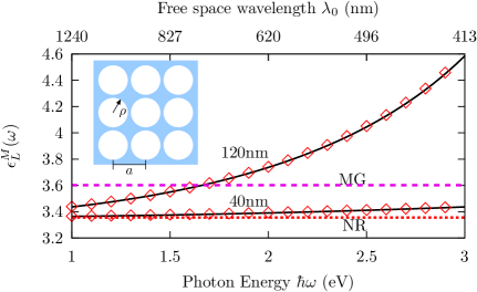
Figure 1: (Color online) Longitudinal macroscopic dielectric function $\epsilon^{M}_{L}(\omega)$ of a 2D system (inset) made up of a square array with lattice parameter $a$ of empty cylindrical holes ($\epsilon_{B}=1$) of circular cross section with radius $\rho=0.45a$ within a dielectric medium with permittivity $\epsilon_{A}=12$. We show the results of using Maxwell-Garnett formula (MG), of a nonretarded calculation (NR), of a numerically exact matrix calculation (diamonds) and of our theory (solid lines) for two different lattice parameters $a=40$nm and $120$nm.

In this calculation we took the limit $\mathbf{k}\to\mathbf{0}$ along the $x$ direction, and we introduced the Cartesian unit vectors $\mathbf{x}$, $\mathbf{y}$ and $\mathbf{z}$. We remark that it is important to assign a direction to $\mathbf{k}$ even in this limit, as the transverse $T$ and longitudinal $L$ projection of $\mathcal{W}^{M}$ differ, although, for this system, the resulting $\epsilon^{M}(\omega)=\epsilon^{M}(\omega,\mathbf{k}\to\mathbf{0})$ is isotropic within the $xy$ plane.

In Fig. 1 we show $\epsilon^{M}_{L}(\omega)$ calculated for two different lattice parameters $a=40$nm and $a=120$nm. Our calculations were performed using the Perl Data Language [45] . The figure shows that our formalism yields the same results as a full straightforward matricial calculation [30] that solves Maxwell equations in a plane wave basis. Nevertheless, our calculation is much more economical in memory usage, as we don’t have to store the full matrices that represent the dynamics of the system, and is at least four orders of magnitude faster as we do not perform any matrix manipulation with our scheme. To illustrate the effects of retardation, in the figure we also show the result of using the non-retarded calculation of Ref. [26] (NR), together with those of the well-know 2D Maxwell-Garnet (MG) effective medium formula [19]. As the dielectric functions of the components are independent of the frequency, since the constituents were taken to be non-dispersive, in this case the frequency dependence of the result arises solely from to the finite ratio of the free space wavelength to the lengthscale of the system, namely, the lattice parameter $a$. Thus, in the $\omega\to 0$ limit our results approach those of the NR calculation. The difference between the NR and MG calculations is due to the high filling fraction $f\approx 0.64$ of the cylinders, which interact non-dipolarly with their nearest neighbors which they almost touch, while MG contains only dipolar interactions. Naturally, retardation effects become stronger as $a$ increases. Furthermore, $\epsilon^{M}(\omega,\mathbf{k})$ depends only on the products $qa$ and $\mathbf{k}a$ so that the two curves shown in Fig. 1 could be collapsed into one curve if appropriately plotted. We use this in Fig. 2, which shows the transverse response $\epsilon^{M}_{T}(\omega,\mathbf{k}_{\Delta})=\epsilon^{M}_{zz}(\omega,\mathbf{k}_{\Delta})$ corresponding to out-of-plane or TE polarization as a function of the normalized frequency $qa/2\pi$. Here, we have chosen a finite in-plane wavevector $\mathbf{k}_{\Delta}=(\pi/2a,0,0)$, corresponding to the midpoint of the $\Delta$ line between $\Gamma$ and $X$ in the first Brillouin zone (BZ) [39]. This figure covers a larger frequency range than Fig. 1, and therefore it displays a series of poles related to resonant multiple coherent reflections at the interfaces between the A and B regions.

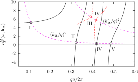
Figure 2: (Color online) Out-of-plane macroscopic dielectric function $\epsilon^{M}_{T}(\omega,\mathbf{k}_{\Delta})$ of the same system as in Fig. 1 for a given wavevector $\mathbf{k}_{\Delta}$ along the $\Delta$ line of the first Brillouin zone (solid lines). The line $(k_{\Delta}/q)^{2}$ (long dashes) intersects (circles) $\epsilon^{M}_{T}(\omega,\mathbf{k}_{\Delta})$ at the frequencies $\omega_{\alpha}(\mathbf{k}_{\Delta})$ of the TE normal modes, with $\alpha=$I, II, IV, V. The intersections (diamonds) of $\epsilon^{M}_{T}(\omega,\mathbf{k}^{\prime}_{\Delta})$ (short dashes) with $(k^{\prime}_{\Delta}/q)^{2}$ (long dashes) corresponding to a shifted wavevector $\mathbf{k}^{\prime}_{\Delta}=\mathbf{k}_{\Delta}+(2\pi/a)\mathbf{y}$ yields the modes $\alpha=$III, IV (see text).

The dispersion relation of transverse waves with TE polarization propagating along the $xy$ plane can be simply written as [46]

$$\epsilon^{M}_{T}(\omega,\mathbf{k})=\frac{k^{2}}{q^{2}}.$$ (26)

Therefore, in Fig. 2 we also plotted the curve $(k_{\Delta}/q)^{2}$. Those points where it intersects the curves for $\epsilon^{M}_{T}$ correspond to normal TE modes of the system with frequencies $\omega_{\alpha}(\mathbf{k}=\mathbf{k}_{\Delta})$, $\alpha=$I, II, …Here, we use roman numerals to number the modes in increasing frequency order.

In Fig. 3 we show the photonic bands (circles) of the TE modes of our system obtained by solving the dispersion relation (26) as $\mathbf{k}$ travels along the line $\Gamma-\Delta-X-Z-M-\Sigma-\Gamma$ within the first BZ.

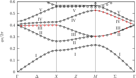
Figure 3: (Color online) Photonic bands of the TE modes of the same system as in Fig. 1 obtained by solving Eq. (26) (circles). For comparison, we also show the photonic bands obtained from the solution of the corresponding eigenvalue problem, Eq. (27), as described in the text (solid lines). We also show the modes obtained by shifting the wavevector $\mathbf{k}\to\mathbf{k}^{\prime}=\mathbf{k}+(2\pi/a)\mathbf{y}$ (diamonds).

In order to test our theory, we also plot the TE modes obtained by solving the eigenvalue equation [47]

$$\left(\frac{1}{\sqrt{\epsilon(\mathbf{r})}}\nabla^{2}\frac{1}{\sqrt{\epsilon(\mathbf{r})}}\right)\left(\sqrt{\epsilon(\mathbf{r})}E_{z}(\mathbf{r})\right)=-\frac{\omega^{2}}{c^{2}}\left(\sqrt{\epsilon(\mathbf{r})}E_{z}(\mathbf{r})\right)$$ (27)

through an implicitly restarted Arnoldi iteration [48] , applying $1/\sqrt{\epsilon(\mathbf{r})}$ in real space and $\nabla\to i(\mathbf{k}+\mathbf{G})$ in reciprocal space [38]. We further verified our results by recalculating them with the freely available package MPB [50] and comparing it to previous results [44] for the same system. The agreement between these calculations shows that it is feasible to use the macroscopic dielectric response of the system to obtain its photonic band structure. However, to succeed, we have to account fully for the spatial dispersion of $\epsilon^{M}_{T}(\omega,\mathbf{k})$.

We remark that although we obtained the correct photonic bands even for large wavevectors, going all the way around the first BZ, there are some regions where we failed to obtain all of the normal modes. For example, our procedure did not produce the third band (labeled III in the figure) along the $\Delta$ line, and neither the fourth band (IV) along the $\Sigma$ line, between $M$ and $\Gamma$. Furthermore, it did not yield the second band (II) which is almost degenerate with the third band (III) along $\Sigma$. It is easily shown that the microscopic field corresponding to the missing band along $\Delta$ is antisymmetric with respect to the reflection $G_{y}\leftrightarrow-G_{y}$ about the $\Delta$ line. Similarly, the missing bands along the region $\Sigma$ are antisymmetric with respect to the reflection $G_{x}\leftrightarrow G_{y}$ about the $\Sigma$ line. Thus, the reciprocal vector $\mathbf{0}$ does not contribute to the electric field for those bands [51], i.e., the missing modes have no macroscopic field components and thus, apparently they may not be obtained from the roots of the macroscopic dispersion relation (26).

Nevertheless, within our formalism, the wavevector $\mathbf{k}$ is actually not restricted to lie within the first BZ. Thus, we may calculate the macroscopic dielectric function for wavevectors beyond the first BZ, and obtain the modes in the extended scheme. In Fig. 2 we show part of the macroscopic dielectric function $\epsilon^{M}_{T}(\omega,\mathbf{k}^{\prime}_{\Delta})$ with a wavevector that has been shifted out of the first BZ from $\mathbf{k}_{\Delta}$ along the $y$ direction by the reciprocal vector $(2\pi/a)\mathbf{y}$, i.e., $\mathbf{k}^{\prime}_{\Delta}=\mathbf{k}_{\Delta}+(2\pi/a)\mathbf{y}$. We remark that $\epsilon^{M}(\omega,\mathbf{k})$ is not a periodic function of $\mathbf{k}$, as it corresponds to a specific plane wave, not to a microscopic Bloch’s wave. The intersection of the curve $(k^{\prime}_{\Delta}/q)^{2}$ with $\epsilon^{M}_{T}(\omega,\mathbf{k}^{\prime}_{\Delta})$ yields the corresponding macroscopic modes. For example, the diamonds in Fig. 2 illustrate two of the normal modes that could be obtained using this shifting procedure. One of these modes is identical to the mode labelled IV that was obtained previously using the unshifted response $\epsilon^{M}_{T}(\omega,\mathbf{k}_{\Delta})$. Nevertheless, another mode, labelled III appears just below $qa/2\pi=0.4$ and it corresponds to one of the previously missing modes. We may shift it back into the first BZ in order to display it in the reduced zone scheme. Proceeding in this fashion, we have obtained all of the previously missing bands, shown by diamonds in Fig. 3. Thus, we have shown that we can calculate the full photonic band structure for the TE modes from the macroscopic non-local dielectric function of the composite system.

A similar procedure to that discussed above can be employed also for the TM modes of the system, with the electric field within the $xy$ plane. In Fig. 4

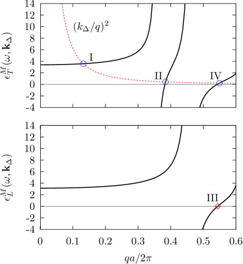
Figure 4: (Color online) In-plane macroscopic dielectric functions $\epsilon^{M}_{T}(\omega,\mathbf{k}_{\Delta})$ (upper panel) and $\epsilon^{M}_{L}(\omega,\mathbf{k}_{\Delta})$ (lower panel) of the same system as in Fig. 1 for the same wavevector $\mathbf{k}_{\Delta}$ as in Fig. 2. The line $(k_{\Delta}/q)^{2}$ (dashes) intersects (circles) $\epsilon^{M}_{T}(\omega,\mathbf{k}_{\Delta})$ at the frequencies $\omega_{\alpha}(\mathbf{k}_{\Delta})$ of the TM transverse normal modes, with $\alpha=$I, II, IV. The zeroes (diamonds) of $\epsilon^{M}_{L}(\omega,\mathbf{k}_{\Delta})$ yield the longitudinal mode III (see text).

we show the in-plane macroscopic dielectric functions $\epsilon^{M}_{xx}(\omega,\mathbf{k}_{\Delta})$ and $\epsilon^{M}_{yy}(\omega,\mathbf{k}_{\Delta})$ of the system for the same wavevector $\mathbf{k}_{\Delta}$ as in Fig. 2. This wavevector and the system are symmetric under $y\leftrightarrow-y$ reflections. Therefore, $\epsilon^{M}_{xy}=0$ and we may identify the transverse and longitudinal responses as $\epsilon^{M}_{T}(\omega,\mathbf{k}_{\Delta})=\epsilon^{M}_{yy}(\omega,\mathbf{k}_{\Delta})$ and $\epsilon^{M}_{L}(\omega,\mathbf{k}_{\Delta})=\epsilon^{M}_{xx}(\omega,\mathbf{k}_{\Delta})$ respectively. The normal modes are then obtained from the transverse dispersion relation (26) and the longitudinal dispersion relation [46]

$$\epsilon^{M}_{L}(\omega,\mathbf{k})=0.$$ (28)

These are identified with circles and diamonds in the figure.

In Fig. 5 we do a similar calculation but along the $\Sigma$ line, for the wavevector $\mathbf{k}_{\Sigma}=(\pi/2a,\pi/2a)$. Along this line, the wavevector and the system are symmetric under the reflection $x\leftrightarrow y$, and thus $\epsilon^{M}_{xx}(\omega,\mathbf{k}_{\Sigma})=\epsilon^{M}_{yy}(\omega,\mathbf{k}_{\Sigma})$. We may now identify the transverse and longitudinal responses as $\epsilon^{M}_{T}(\omega,\mathbf{k}_{\Sigma})=\epsilon^{M}_{xx}(\omega,\mathbf{k}_{\Sigma})-\epsilon^{M}_{xy}(\omega,\mathbf{k}_{\Sigma})$ and $\epsilon^{M}_{L}(\omega,\mathbf{k}_{\Sigma})=\epsilon^{M}_{xx}(\omega,\mathbf{k}_{\Sigma})+\epsilon^{M}_{xy}(\omega,\mathbf{k}_{\Sigma})$ respectively. The upper panel of Fig. 5 shows $\epsilon^{M}_{T}(\omega,\mathbf{k}_{\Sigma})$, $(k_{\Sigma}/q)^{2}$ and their intersections (circles) which yield the transverse modes, while the lower panel displays $\epsilon^{M}_{L}(\omega,\mathbf{k}_{\Sigma})$ and its zero (diamond) which correspond to a longitudinal mode.

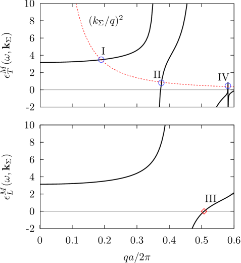
Figure 5: (Color online) In-plane macroscopic dielectric functions $\epsilon^{M}_{T}(\omega,\mathbf{k}_{\Sigma})$ (upper panel) and $\epsilon^{M}_{L}(\omega,\mathbf{k}_{\Sigma})$ (lower panel) of the same system as in Fig. 1 for a given wavevector $\mathbf{k}_{\Sigma}$ along the $\Sigma$ line. The line $(k_{\Sigma}/q)^{2}$ (dashes) intersects (circles) $\epsilon^{M}_{T}(\omega,\mathbf{k}_{\Sigma})$ at the frequencies $\omega_{\alpha}(\mathbf{k}_{\Sigma})$ of the TM transverse normal modes, with $\alpha$=I, II, IV. The zeroes (diamonds) of $\epsilon^{M}_{L}(\omega,\mathbf{k}_{\Sigma})$ yield the longitudinal mode III (see text).

Along the $Z$ line, from $X$ to $M$, there is no crystal symmetry operation that leaves invariant the wavevector, and thus transverse and longitudinal fields mix among themselves, i.e., there are no longitudinal nor transverse modes. Nevertheless, we may obtain the frequencies of the mixed modes through the singularities of the wave operator matrix

$$\det\left[\mathcal{W}^{M}(\omega,\mathbf{k})\right]=0,$$ (29)

as illustrated in Fig. 6

Figure 6: Determinant of the macroscopic wave operator matrix $\mathcal{W}^{M}(\omega,\mathbf{k}_{Z})$ for a given wavevector $\mathbf{k}_{Z}$ along the $Z$ line. The normal modes of the system $\omega_{\alpha}(\mathbf{k}_{Z})$, $\alpha=$I, II, III, IV, correspond to its zeroes (squares).

for a wavevector $\mathbf{k}_{Z}=(\pi/a,\pi/2a)$ along the $Z$ line.

From calculations such as those illustrated by Figs. 4, 5 and 6, or more generally, from the zeroes of $\det\left[\mathcal{W}^{M}(\omega,\mathbf{k})\right]$ for arbitrary wavevectors $\mathbf{k}$, we can obtain the full TM photonic band structure, as shown by Fig. 7.

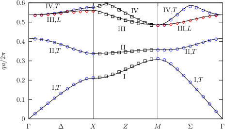
Figure 7: (Color online) Photonic bands of the TM modes of the same system as in Fig. 1. The modes between $\Gamma$ and $X$ and between $M$ and $\Gamma$ may be obtained by solving Eq. (26) for the transverse ($T$) modes (circles) and Eq. (28) for the longitudinal ($L$) modes (diamonds), or Eq. (29) for both of them. The modes from $X\to M$ are obtained from Eq. (29) and have a mixed polarization (squares). For comparison, we also show the photonic bands obtained from the solution of the corresponding eigenvalue problem, Eq. (30), as described in the text (solid lines).

In order to test our theory, we also plot the TM modes obtained by solving the eigenvalue equation [47]

$$\nabla\cdot\frac{1}{\epsilon(\mathbf{r})}\nabla B_{z}(\mathbf{r})=-\frac{\omega^{2}}{c^{2}}B_{z}(\mathbf{r})$$ (30)

using similar methods [48, 38] as for the TE case and comparing them successfully to previous results [44] for the same system. The agreement between these calculations shows that it is also feasible to use the macroscopic dielectric response of the system to obtain its photonic band structure in the TM case.

An approximate band structure could be obtained for transverse waves in the region of small wavevectors $\mathbf{k}\to\mathbf{0}$ by expanding the LHS of Eq. (26) up to second order in $k$ and solving for $k^{2}$. The result is a local dispersion relation

$$k^{2}=q^{2}\epsilon^{M}(\omega)\mu(\omega),$$ (31)

where the non-locality of $\epsilon^{M}_{T}(\omega,\mathbf{k})$ is partially accounted for through an effective magnetic permeability [23]

$$\mu(\omega)=\left.\frac{1}{1-\frac{q^{2}}{2}\frac{\partial^{2}}{\partial k^{2}}\epsilon^{M}_{T}(\omega,k\mathbf{x})}\right|_{k=0}.$$ (32)

In Fig. 8 we show the resulting approximate bands for the TE case.

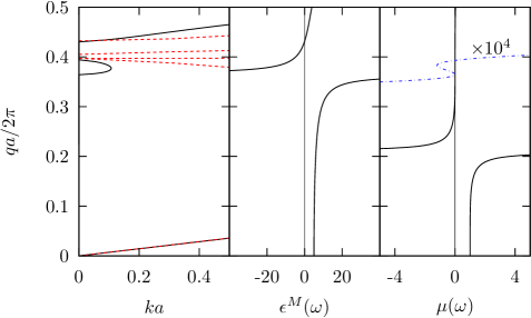
Figure 8: Local dispersion relation for the same system as in Fig. 1 for the TE case (solid lines, left panel), obtained from Eq. (31). Local dielectric function $\epsilon^{M}(\omega)$ (middle panel). Local magnetic permeability $\mu(\omega)$ (solid line, right panel) and $10^{4}\mu(\omega)$ (dash-dotted line, right panel). For comparison purposes, we also show the exact dispersion relation (dashed line, left panel).

We can see that the acoustic band within the local approximation is indistinguishable from the exact result for small wavevectors. This local acoustic band extends up to the frequency $qa/2\pi\approx 0.2$ for which $\mu$ has a pole. The local approximation also reproduces the upper band of the exact calculation (labelled V in Fig. 3), but only in the immediate vicinity of $\Gamma$, close to the zero $qa/2\pi\approx 0.43$ of $\epsilon^{M}(\omega)$. For larger wavevectors it acquires a larger positive dispersion. As discussed above, the band labelled III in Fig. 3 doesn’t couple to macroscopic fields for $\mathbf{k}$ along the $\Delta$ line, while the band labelled IV doesn’t couple along the $\Sigma$ line. Thus, neither band couples to macroscopic fields at $\Gamma$ and as a consequence, these bands are not reproduced at all by the local approximation (31).

In the region $qa/2\pi\approx 0.36-0.40$ the local approximation predicts a curious band that displays backbending. Its lower part begins at the pole of $\epsilon^{M}(\omega)$, which corresponds to a double zero of $\mu(\omega)$ [38]. This part of the local dispersion relation is spurious, as the second order Taylor expansion of the dielectric function that yields Eqs. (32) and (31) starting from Eq. (26) would be meaningless at a pole. Consequently, this part of the local band doesn’t correspond to any band within the exact calculation. On the other hand, the upper part of the backbending band starts at a simple zero of $\mu$ which arises from a different kind of singular behavior, consisting of a pole in $\epsilon^{M}_{T}(\omega,\mathbf{k})$ at $qa/2\pi\approx 0.40$ which is suppressed at $k=0$ as its weight is approximately proportional to $k^{2}$. This part of the local dispersion relation agrees with band II of Fig. 3 at $\Gamma$ and displays a negative dispersion as does band II. Furthermore, for this band, both $\epsilon^{M}$ and $\mu$ are negative. Thus, our photonic crystal, made up of holes within a dispersionless dielectric, behaves for some frequencies as a left-handed metamaterial [52, 53]. Nevertheless, caution should be exercised when using Eqs. (32) and (31) close to singularities of $\epsilon^{M}_{T}(\omega,\mathbf{k})$.

6 Conclusions

We have shown that the macroscopic inverse wave operator of composite systems with arbitrary spatial fluctuations is simply given by the average projection of the corresponding microscopic operator. These operators may be related to the macroscopic and macroscopic dielectric functions, thus yielding a general procedure to incorporate the effects of spatial fluctuations in the calculation of all the components of the macroscopic dielectric tensor of the system. We have extended Haydock’s recursive scheme in order to calculate very efficiently the response of periodic two-component systems in terms of a continued fraction whose coefficients may be obtained without recourse to operations with the large matrices that characterize the microscopic response and the field equations. We illustrated and tested our results through the calculation of the wavevector and frequency dependent macroscopic dielectric tensor of a 2D dielectric system with non-dispersive non-dissipative components. We identified the transverse and longitudinal components of the response for wavevectors along symmetry lines and we obtained all the components of the tensorial response for the case of reduced symmetry. The macroscopic response has a series of poles, related to resonant multiple coherent reflections and by accounting for its spatial dispersion we obtained the full photonic band structure of the system from the dispersion relations corresponding to the homogenized material. Besides yielding the correct bands from a macroscopic approach, our scheme allowed us to classify the polarization of each mode as either transverse, longitudinal or mixed. Even though the macroscopic approach might fail to yield some modes, namely, those which have no coupling to the macroscopic field due to symmetry, they may be recovered by extending the notion of macroscopic state, allowing its wavevector to lie beyond the first Brillouin zone. The non-locality of the dielectric response may be partially accounted for through a magnetic permeability which can then be employed in the calculation of the optical properties of the system. We compared the band structure obtained through this local approximation to the exact results and we obtained partial agreement close to $\Gamma$ for those bands that do couple to long-wavelentgh fields. In particular, we showed that this approach can yield a negative dispersion in frequency regions where both the permitivity and permeability are negative. Nevertheless, we discussed some shortcommings of the local approach. Although here we presented results for dispersionless transparent dielectrics, our calculation does not require that the materials that make up the system be non-dispersive nor non-dissipative, so that calculations for real dielectrics and metals may be performed with the same low computational costs.

References

References

- [1] M. Brédov, V. Rumiantsev, and L. Toptiguin. Classical electrodynamics. Mir Moscow, 1985.
- [2] M. Notomi. Theory of light propagation in strongly modulated photonic crystals: Refractionlike behavior in the vicinity of the photonic band gap. Phys. Rev. B, 62:10696–10705, Oct 2000.
- [3] Rubén G. Barrera, Alejandro Reyes-Coronado, and Augusto García-Valenzuela. Nonlocal nature of the electrodynamic response of colloidal systems. Phys. Rev. B, 75:184202, May 2007.
- [4] Pochi Yeh, Amnon Yariv, and Chi-Shain Hong. Electromagnetic propagation in periodic stratified media. i. general theory. J. Opt. Soc. Am., 67(4):423–438, Apr 1977.
- [5] W. Luis Mochán and Rubén G. Barrera. Electromagnetic response of systems with spatial fluctuations. I. General formalism. Phys. Rev. B, 32(8):4984–4988, Oct 1985.
- [6] W. Luis Mochán and Rubén G. Barrera. Electromagnetic response of systems with spatial fluctuations. II. Applications. Phys. Rev. B, 32(8):4989–5001, Oct 1985.
- [7] Hideo Kosaka, Takayuki Kawashima, Akihisa Tomita, Masaya Notomi, Toshiaki Tamamura, Takashi Sato, and Shojiro Kawakami. Superprism phenomena in photonic crystals. Phys. Rev. B, 58:R10096–R10099, Oct 1998.
- [8] D. Stroud and F. P. Pan. Self-consistent approach to electromagnetic wave propagation in composite media: Application to model granular metals. Phys. Rev. B, 17:1602–1610, Feb 1978.
- [9] G.P. Ortiz and W.L. Mochán. Scaling of light scattered from fractal aggregates at resonance. Phys. Rev. B., 67(184204), 2003.
- [10] G.P. Ortiz and W.L. Mochán. Scaling condition for multiple scattering in fractal aggregates. Physica B, 338:54, 2003.
- [11] M. Hilke. Seeing anderson localization. Phys. Rev. A, 80:063820, Dec 2009.
- [12] Jiabi Chen, Yan Wang, Baohua Jia, Tao Geng, Xiangping Li, Lie Feng, Wei Qian, Bingming Liang, Xuanxiong Zhang, Min Gu, and Songlin and Zhuang. Observation of the inverse doppler effect in negative-index materials at optical frequencies. P Nat Photon, 5(4):239–245, 2011.
- [13] Baile Zhang, Yuan Luo, Xiaogang Liu, and George Barbastathis. Macroscopic invisibility cloak for visible light. Phys. Rev. Lett., 106:033901, Jan 2011.
- [14] Henri J. Lezec, Jennifer A. Dionne, and Harry A. Atwater. Negative refraction at visible frequencies. Science, 316(5823):430–432, 2007.
- [15] Yaroslav A. Urzhumov and Gennady Shvets. Optical magnetism and negative refraction in plasmonic metamaterials. Solid State Communications, 146(5 6):208 – 220, 2008. ¡ce:title¿Special section on Negative Refraction and Metamaterials for Optical Science and Engineering¡/ce:title¿.
- [16] G. W. Milton, R. C. McPhedran, and D. R. McKenzie. Transport properties of arrays of intersecting cylinders. Applied Physics A: Materials Science and Processing, 25(1):23–30, 1981.
- [17] David J. Bergman and Keh-Jim Dunn. Bulk effective dielectric constant of a composite with a periodic microgeometry. Phys. Rev. B, 45(23):13262–13271, Jun 1992.
- [18] Ruibao Tao, Zhe Chen, and Ping Sheng. First-principles fourier approach for the calculation of the effective dielectric constant of periodic composites. Phys. Rev. B, 41(4):2417–2420, Feb 1990.
- [19] S. Datta, C. T. Chan, K. M. Ho, and C. M. Soukoulis. Effective dielectric constant of periodic composite structures. Phys. Rev. B, 48(20):14936–14943, Nov 1993.
- [20] A. Alexopoulos. Effective-medium theory of surfaces and metasurfaces containing two-dimensional binary inclusions. Phys. Rev. E, 81(4):046607, Apr 2010.
- [21] William T. Doyle. Optical properties of a suspension of metal spheres. Phys. Rev. B, 39(14):9852–9858, May 1989.
- [22] Alon Ludwig and Kevin J. Webb. Accuracy of effective medium parameter extraction procedures for optical metamaterials. Phys. Rev. B, 81(11):113103, Mar 2010.
- [23] João T. Costa, Mário G. Silveirinha, and Stanislav I. Maslovski. Finite-difference frequency-domain method for the extraction of effective parameters of metamaterials. Phys. Rev. B, 80:235124, Dec 2009.
- [24] G.P. Ortiz, C.López-Bastidas, J.A.Maytorena, and W.L.Mochán. Bulk response of composite from finite samples. Physica B, 338:103, 2003.
- [25] Mário G. Silveirinha. Nonlocal homogenization model for a periodic array of -negative rods. Phys. Rev. E, 73:046612, Apr 2006.
- [26] W. Luis Mochan, Guillermo P. Ortiz, and Bernardo S. Mendoza. Efficient homogenization procedure for the calculation of optical properties of 3d nanostructured composites. Opt. Express, 18(21):22119–22127, Oct 2010.
- [27] V. Myroshnychenko and C. Brosseau. Analysis of the effective permittivity in percolative composites using finite element calculations. Physica B: Condensed Matter, 405(14):3046 – 3049, 2010. Proceedings of the Eighth International Conference on Electrical Transport and Optical Properties of Inhomogeneous Media; ETOPIM-8.
- [28] S. Guenneau, F. Zolla, and A. Nicolet. Homogenization of 3d finite photonic crystals with heterogeneous permittivity and permeability. Waves in Random and Complex Media, 17(4):653–697, 2007.
- [29] A. I. Căbuz, A. Nicolet, F. Zolla, D. Felbacq, and G. Bouchitté. Homogenization of nonlocal wire metamaterial via a renormalization approach. J. Opt. Soc. Am. B, 28(5):1275–1282, May 2011.
- [30] Guillermo P. Ortiz, Brenda E. Martínez-Zérega, Bernardo S. Mendoza, and W. Luis Mochán. Effective optical response of metamaterials. Phys. Rev. B, 79(24):245132, Jun 2009.
- [31] Shreyas B. Raghunathan and Neil V. Budko. Effective permittivity of finite inhomogeneous objects. Phys. Rev. B, 81:054206, Feb 2010.
- [32] P. Halevi, A. A. Krokhin, and J. Arriaga. Photonic crystal optics and homogenization of 2d periodic composites. Phys. Rev. Lett., 82:719–722, Jan 1999.
- [33] P. Halevi and F. Pérez-Rodríguez. From photonic crystals (via homogenization) to metamaterials. In Society of Photo-Optical Instrumentation Engineers (SPIE) Conference Series, volume 6320 of Society of Photo-Optical Instrumentation Engineers (SPIE) Conference Series, August 2006.
- [34] C R Simovski. On electromagnetic characterization and homogenization of nanostructured metamaterials. Journal of Optics, 13(1):013001, 2011.
- [35] Christoph Menzel, Thomas Paul, Carsten Rockstuhl, Thomas Pertsch, Sergei Tretyakov, and Falk Lederer. Validity of effective material parameters for optical fishnet metamaterials. Phys. Rev. B, 81(3):035320, Jan 2010.
- [36] John David Jackson. Classical Electrodynamics. Wiley, 1998.
- [37] W. Luis Mochan. Plasmons. Encyclopaedia of Condensed Matter Physics, 310, 2005.
- [38] J.S. Pérez-Huerta, Bernardo S. Mendoza, Guillermo Ortiz, and W. Luis Mochán. Conducting metamaterials. In preparation.
- [39] Kazuaki. Sakoda. Optical Properties of Photonic Crystals. Springer Series in Optical Sciences. Springer, 2004.
- [40] Adrian P. Sutton. Electronic Structure of Materials. Oxford, 2004.
- [41] Supriyo. Datta. Electronic Transport in Mesoscopic Systems. Cambridge Studies in Semiconductor Physics and Microelectronic Engineering. Cambridge University Press, 1997.
- [42] R Haydock, V Heine, and M J Kelly. Electronic structure based on the local atomic environment for tight-binding bands. Journal of Physics C: Solid State Physics, 5(20):2845, 1972.
- [43] R Haydock, V Heine, and M J Kelly. Electronic structure based on the local atomic environment for tight-binding bands. ii. Journal of Physics C: Solid State Physics, 8(16):2591, 1975.
- [44] K. Busch, G. von Freymann, S. Linden, S.F. Mingaleev, L. Tkeshelashvili, and M. Wegener. Periodic nanostructures for photonics. Physics Reports, 444(3–6):101 – 202, 2007.
- [45] K. Glazebrook and F. Economou. Pdl: The perl data language. Dr. Dobb’s Journal, 1997.
- [46] L.D. Landau and E.M. Lifshits. Electrodynamics of continuous media. Course of theoretical physics. Pergamon Press Ltd., 1984.
- [47] J.D. Joannopoulos, R.D. Meade, and J.N. Winn. Photonic Crystals: Molding the Flow of Light. University Press, 1995.
- [48] Yousef Saad. Numerical methods for large eigenvalues problems. SIAM, 2011.
- [49] W. Luis Mochán, Bernardo S. Mendoza, J.S. Pérez-Huerta, and Guillermo Ortiz. The implicitly restarted arnoldi iteration for the calculations of photonics band. In preparation.
- [50] Steven G. Johnson and J. D. Joannopoulos. Block-iterative frequency-domain methods for maxwell’s equations in a planewave basis. Opt. Express, 8(3):173–190, 2001.
- [51] W. M. Robertson and G. Arjavalingam. Measeuremen of photonic band structure in a two-dimensional periodic dielectric array. Phys. Rev. Lett., 68(13):2023, 1992.
- [52] Liang Peng, Lixin Ran, Hongsheng Chen, Haifei Zhang, Jin Au Kong, and Tomasz M. Grzegorczyk. Experimental observation of left-handed behavior in an array of standard dielectric resonators. Phys. Rev. Lett., 98:157403, Apr 2007.
- [53] K. Vynck, D. Felbacq, E. Centeno, A. I. Căbuz, D. Cassagne, and B. Guizal. All-dielectric rod-type metamaterials at optical frequencies. Phys. Rev. Lett., 102:133901, Mar 2009.