Optimal scaling for the transient phase of Metropolis Hastings algorithms: The longtime behavior

Abstract

We consider the Random Walk Metropolis algorithm on $\mathbb{R}^{n}$ with Gaussian proposals, and when the target probability measure is the $n$-fold product of a one-dimensional law. It is well known (see Roberts et al. (Ann. Appl. Probab. 7 (1997) 110–120)) that, in the limit $n\to\infty$, starting at equilibrium and for an appropriate scaling of the variance and of the timescale as a function of the dimension $n$, a diffusive limit is obtained for each component of the Markov chain. In Jourdain et al. (Optimal scaling for the transient phase of the random walk Metropolis algorithm: The mean-field limit (2012) Preprint), we generalize this result when the initial distribution is not the target probability measure. The obtained diffusive limit is the solution to a stochastic differential equation nonlinear in the sense of McKean. In the present paper, we prove convergence to equilibrium for this equation. We discuss practical counterparts in order to optimize the variance of the proposal distribution to accelerate convergence to equilibrium. Our analysis confirms the interest of the constant acceptance rate strategy (with acceptance rate between $1/4$ and $1/3$) first suggested in Roberts et al. (Ann. Appl. Probab. 7 (1997) 110–120).

We also address scaling of the Metropolis-Adjusted Langevin Algorithm. When starting at equilibrium, a diffusive limit for an optimal scaling of the variance is obtained in Roberts and Rosenthal (J. R. Stat. Soc. Ser. B. Stat. Methodol. 60 (1998) 255–268). In the transient case, we obtain formally that the optimal variance scales very differently in $n$ depending on the sign of a moment of the distribution, which vanishes at equilibrium. This suggest that it is difficult to derive practical recommendations for MALA from such asymptotic results.

, and

1 Introduction

Many Markov Chain Monte Carlo (MCMC) methods are based on the Metropolis–Hastings algorithm, see [16, 13]. To set up the notation, let us recall this well-known sampling technique. Let us consider a target probability distribution on $\mathbb{R}^{n}$ with density $p$. Starting from an initial random variable $X_{0}$, the Metropolis–Hastings algorithm generates iteratively a Markov chain $(X_{k})_{k\geq 0}$ in two steps. At time $k$, given $X_{k}$, a candidate $Y_{k+1}$ is sampled using a proposal distribution with density $q(X_{k},y)$. Then, the proposal $Y_{k+1}$ is accepted with probability $\alpha(X_{k},Y_{k+1})$, where

$$\alpha(x,y)=1\wedge\frac{p(y)q(y,x)}{p(x)q(x,y)}.$$

Here and in the following, we use the standard notation $a\wedge b=\min(a,b)$. If the proposed value is accepted, then $X_{k+1}=Y_{k+1}$ otherwise $X_{k+1}=X_{k}$. The Markov Chain $(X_{k})_{k\geq 0}$ is by construction reversible with respect to the target density $p$, and thus admits $p$ as an invariant distribution. The efficiency of this algorithm highly depends on the choice of the proposal distribution $q$. One common choice is a Gaussian proposal centered at point $x\in\mathbb{R}^{n}$ with variance $\sigma^{2}\mathrm{Id}_{n\times n}$:

$$q(x,y)=\frac{1}{(2\uppi\sigma^{2})^{n/2}}\exp\biggl{(}-\frac{|x-y|^{2}}{2\sigma^{2}}\biggr{)}.$$

Since the proposal is symmetric ($q(x,y)=q(y,x)$), the acceptance probability reduces to

$$\alpha(x,y)=1\wedge\frac{p(y)}{p(x)}.$$ (1)

Metropolis–Hastings algorithms with symmetric kernels are called random walk Metropolis (RWM). Another popular choice yields the so called Metropolis adjusted Langevin algorithm (MALA). In this case, the proposal distribution is a Gaussian random variable with variance $\sigma^{2}\mathrm{Id}_{n\times n}$ and centered at point $x+\frac{\sigma^{2}}{2}\nabla\ln(p(x))$ (in particular, it is not symmetric). It corresponds to one step of a time-discretization with timestep $\sigma^{2}$ of the (overdamped) Langevin dynamics: $\mathrm{d}X_{t}=\mathrm{d}B_{t}+\frac{1}{2}\nabla\ln p(X_{t})\,\mathrm{d}t$ which is ergodic with respect to $p(x)\,\mathrm{d}x$ (here, $B_{t}$ is a standard $n$-dimensional Brownian motion).

In both cases (RWM and MALA), the variance $\sigma^{2}$ remains to be chosen. It should be sufficiently large to ensure a good exploration of the state space, but not too large otherwise the rejection rate becomes typically very high since the proposed moves fall in low probability regions, in particular in high dimension. It is expected that the higher the dimension, the smaller the variance of the proposal should be. The first theoretical results to optimize the choice of $\sigma^{2}$ in terms of the dimension $n$ can be found in [22]. The authors study the RWM algorithm under two fundamental (and somewhat restrictive) assumptions: (i) the target probability distribution is the $n$-fold tensor product of a one-dimensional density:

$$p(x)=\prod_{i=1}^{n}\exp\bigl{(}-V(x_{i})\bigr{)},$$ (2)

where $x=(x_{1},\ldots,x_{n})$ and $\int_{\mathbb{R}}\exp(-V)=1$, and (ii) the initial distribution is the target probability (what we refer to as the stationarity assumption in the following):

$$X^{n}_{0}\sim p(x)\,\mathrm{d}x.$$

The superscript $n$ in the Markov chain $(X^{n}_{k})_{k\geq 0}$ explicitly indicates the dependency on the dimension $n$. Then, under additional regularity assumption on $V$, the authors prove that for a proper scaling of the variance as a function of the dimension, namely

$$\sigma_{n}^{2}=\frac{\ell^{2}}{n},$$

where $\ell$ is a fixed constant, the Markov process $(X^{1,n}_{\lfloor nt\rfloor})_{t\geq 0}$ (where $X^{1,n}_{k}\in\mathbb{R}$ denotes the first component of $X^{n}_{k}\in\mathbb{R}^{n}$) converges in law to a diffusion process:

$$\mathrm{d}X_{t}=\sqrt{h(I,\ell)}\,\mathrm{d}B_{t}-h(I,\ell){\textstyle\frac{1}{2}}V^{\prime}(X_{t})\,\mathrm{d}t,$$ (3)

where

$$h(I,\ell)=2\ell^{2}\Phi\biggl{(}-\frac{\ell\sqrt{I}}{2}\biggr{)}\quad\mbox{and}\quad I=\int_{\mathbb{R}}\bigl{(}V^{\prime}\bigr{)}^{2}\exp(-V).$$ (4)

Here and in the following, $\lfloor\cdot\rfloor$ denotes the integer part (for $y\in\mathbb{R}$, $\lfloor y\rfloor\in\mathbb{Z}$ and $\lfloor y\rfloor\leq y<\lfloor y\rfloor+1$) and $\Phi$ is the cumulative distribution function of the normal distribution ($\Phi(x)=\frac{1}{\sqrt{2\uppi}}\int_{-\infty}^{x}\exp(-y^{2}/2)\,\mathrm{d}y$). The scalings of the variance and of the time as a function of the dimension are indications on how to make the RWM algorithm efficient in high dimension. Moreover, a practical counterpart of this result is that $\ell$ should be chosen such that $h(I,\ell)$ is maximum (the optimal value of $\ell$ is $\frac{c_{0}}{\sqrt{I}}$ with $c_{0}\simeq 2.38$), in order to optimize the time scaling in (3). This optimal value of $\ell$ corresponds equivalently to a constant average acceptance rate, with approximate value $0.234$: for this choice of $\ell$, in the limit $n$ large,

$$\int\!\!\!\int\alpha(x,y)p(x)q(x,y)\,\mathrm{d}x\,\mathrm{d}y\simeq 0.234.$$

Notice that the optimal average acceptance rate does not depend on $I$, and is thus the same whatever the target probability. Thus, the practical way to choose $\sigma^{2}$ is to scale it in such a way that the average acceptance rate is roughly $1/4$. Similar results have been obtained for the MALA algorithm in [23]. In this case, the scaling for the variance is $\sigma_{n}^{2}=\frac{\ell^{2}}{n^{1/3}}$, the time scaling is $(X^{n}_{\lfloor n^{1/3}t\rfloor})_{t\geq 0}$ and the optimal average acceptance rate is $0.574$.

There exists several extensions of such results for various Metropolis–Hastings algorithms, see [23, 24, 10, 17, 18, 7, 6, 8], and some of them relax in particular the first main assumption mentioned above about the separated form of the target distribution, see [11, 4, 5, 9]. Extensions to infinite dimensional settings have also been explored, see [15, 21, 9].

All these results assume stationarity: the initial measure is the target probability. To the best of the authors’ knowledge, the only works which deal with a nonstationary case are [12] where the RWM and the MALA algorithms are analyzed in the Gaussian case and [20]. In the latter paper, the target measure is assumed to be absolutely continuous with respect to the law of an infinite dimensional Gaussian random field and this measure is approximated in a space of dimension $n$ where the MCMC algorithm is performed. The authors consider a modified RWM algorithm (called preconditioned Crank–Nicolson walk) started at a deterministic initial condition and prove that when $\sigma_{n}$ tends to $0$ as $n$ tends to $\infty$ (with no restriction on the rate of convergence of $\sigma_{n}$ to $0$), the rescaled algorithm converges to a stochastic partial differential equation, started at the same initial condition.

The aim of this article is to discuss extensions of the previous results for the RWM and the MALA algorithms, without assuming stationarity. The main findings are the following.

Concerning the RWM algorithm, in the companion paper [14], we prove that, using the same scaling for the variance and the time as in the stationary case (namely $\sigma_{n}^{2}=\frac{\ell^{2}}{n}$ and considering $(X^{1,n}_{\lfloor nt\rfloor})_{t\geq 0}$), one obtains in the limit $n$ goes to infinity a diffusion process nonlinear in the sense of McKean (see Equation (1) below). This is discussed in Section 2. Contrary to (3), this diffusion process cannot be obtained from the simple Langevin dynamics $\mathrm{d}X_{t}=\mathrm{d}B_{t}-\frac{V^{\prime}(X_{t})}{2}\,\mathrm{d}t$ by a deterministic time-change and its long-time behavior is not obvious. In Section 3, we first prove that its unique stationary distribution is $\mathrm{e}^{-V(x)}\,\mathrm{d}x$. Assuming that this measure satisfies a logarithmic Sobolev inequality, we prove that the Kullback–Leibler divergence of the marginal distribution at time $t$ with respect to $\mathrm{e}^{-V(x)}\,\mathrm{d}x$ converges to $0$ at an exponential rate. In Section 4, we discuss optimizing strategies which take into account the transient phase. Roughly speaking, the usual strategy which consists in choosing $\ell$ (recall that $\sigma_{n}^{2}=\frac{\ell^{2}}{n}$) such that the average acceptance rate is constant (with value between $1/4$ and $1/3$) seems to be a very good strategy. This is numerically illustrated in Section 5.

Concerning the MALA algorithm, the situation is much more complicated. The scaling to be used seems to depend on the sign of an average quantity (see Section 6.1.3). In particular, the scaling $\sigma_{n}^{2}=\frac{\ell^{2}}{n^{1/3}}$ which has been identified in [23] under the stationary assumption is not adapted to the transient phase. It seems difficult to draw any practical recommendation from this analysis. This is explained with details in Section 6.

2 Scaling limit for the RWM algorithm

In this section, we state the diffusion limit for the RWM algorithm, and explain formally why this result holds. A rigorous proof can be found in [14].

2.1 The RWM algorithm and the convergence result

We consider a Random Walk Metropolis algorithm using Gaussian proposal with variance $\sigma_{n}^{2}=\frac{\ell^{2}}{n}$, and with target $p$ defined by (2). The Markov chain generated using this algorithm writes:

$$X^{i,n}_{k+1}=X^{i,n}_{k}+\frac{\ell}{\sqrt{n}}G^{i}_{k+1}1_{{\mathcal{A}}_{k+1}},\qquad 1\leq i\leq n$$ (5)

with

$${\mathcal{A}}_{k+1}=\bigl{\{}U_{k+1}\leq\mathrm{e}^{\sum_{i=1}^{n}(V(X^{i,n}_{k})-V(X^{i,n}_{k}+({\ell}/{\sqrt{n}})G^{i}_{k+1}))}\bigr{\}},$$

where $(G^{i}_{k})_{i,k\geq 1}$ is a sequence of independent and identically distributed (i.i.d.) normal random variables independent from a sequence $(U_{k})_{k\geq 1}$ of i.i.d. random variables with uniform law on $[0,1]$. We assume that the initial positions $(X^{1,n}_{0},\ldots,X^{n,n}_{0})$ are exchangeable (namely the law of the vector is invariant under permutation of the indices) and independent from all the previous random variables. Exchangeability is preserved by the dynamics: for all $k\geq 1$, $(X^{1,n}_{k},\ldots,X^{n,n}_{k})$ are exchangeable. We denote by ${\mathcal{F}}^{n}_{k}$ the sigma field generated by $(X^{1,n}_{0},\ldots,X^{n,n}_{0})$ and $(G^{1}_{l},\ldots,G^{n}_{l},U_{l})_{1\leq l\leq k}$.

For $t>0$ and $i\in\{1,\ldots,n\}$, let

$$Y^{i,n}_{t} = \bigl{(}\lceil nt\rceil-nt\bigr{)}X^{i,n}_{\lfloor nt\rfloor}+\bigl{(}nt-\lfloor nt\rfloor\bigr{)}X^{i,n}_{\lceil nt\rceil}$$

$$= X^{i,n}_{\lfloor nt\rfloor}+\bigl{(}nt-\lfloor nt\rfloor\bigr{)}\frac{\ell}{\sqrt{n}}G^{i}_{\lceil nt\rceil}1_{{\mathcal{A}}_{\lceil nt\rceil}}$$

be the linear interpolation of the Markov chain obtained by rescaling time (the characteristic time scale is $1/n$). This is the classical diffusive time-scale for a random walk, since the variance of each move is of order $1/n$.

Let us define the notion of convergence (namely the propagation of chaos) that will be useful to study the convergence of the interacting particle system $((Y^{1,n}_{t},\ldots,Y^{n,n}_{t})_{t\geq 0})_{n\geq 1}$ in the limit $n$ goes to infinity.

Definition 1.

Let $E$ be a separable metric space. A sequence $(\chi^{n}_{1},\ldots,\chi_{n}^{n})_{n\geq 1}$ of exchangeable $E^{n}$-valued random variables is said to be $\nu$-chaotic where $\nu$ is a probability measure on $E$ if for fixed $j\in\mathbb{N}^{*}$, the law of $(\chi^{n}_{1},\ldots,\chi_{j}^{n})$ converges in distribution to $\nu^{\otimes j}$ as $n$ goes to $\infty$.

According to [25], Proposition 2.2, the $\nu$-chaoticity is equivalent to a law of large numbers result, namely the convergence in probability of the empirical measures $\mu^{n}=\frac{1}{n}\sum_{i=1}^{n}\delta_{\chi^{n}_{i}}$ to the constant $\nu$ when the space of probability measures on $E$ is endowed with the weak convergence topology.

We are now in position to state the convergence result for the RWM algorithm, taken from [14]. Here and in the following, the bracket notation refers to the duality bracket for probability measures on $\mathbb{R}$: for $\mu$ a probability measure and $\phi$ a bounded measurable function,

$$\langle\mu,\phi\rangle=\int\phi\,\mathrm{d}\mu.$$

Theorem 1.

Let $m$ be a probability measure on $\mathbb{R}$ such that $\langle m,(V^{\prime})^{4}\rangle<+\infty$. Let us also assume that

$$V\mbox{ is a }C^{3}\mbox{ function on }\mathbb{R}\mbox{ with bounded second and third order derivatives}.$$ (6)

If the initial positions $(X^{1,n}_{0},\ldots,X^{n,n}_{0})_{n\geq 1}$ are $m$-chaotic and such that

$$\sup_{n}\mathbb{E}\bigl{[}\bigl{(}V^{\prime}\bigl{(}X_{0}^{1,n}\bigr{)}\bigr{)}^{4}\bigr{]}<+\infty,$$

then the processes $((Y^{1,n}_{t},\ldots,Y^{n,n}_{t})_{t\geq 0})_{n\geq 1}$ are $P$-chaotic where $P$ denotes the law (on the space ${\mathcal{C}}(\mathbb{R}_{+},\mathbb{R})$ of continuous function with values in $\mathbb{R}$) of the unique solution to the stochastic differential equation nonlinear in the sense of McKean

$$\mathrm{d}X_{t} = \Gamma^{1/2}\bigl{(}\mathbb{E}\bigl{[}\bigl{(}V^{\prime}(X_{t})\bigr{)}^{2}\bigr{]},\mathbb{E}\bigl{[}V^{\prime\prime}(X_{t})\bigr{]},\ell\bigr{)}\,\mathrm{d}B_{t}$$

$${}-{\mathcal{G}}\bigl{(}\mathbb{E}\bigl{[}\bigl{(}V^{\prime}(X_{t})\bigr{)}^{2}\bigr{]},\mathbb{E}\bigl{[}V^{\prime\prime}(X_{t})\bigr{]},\ell\bigr{)}V^{\prime}(X_{t})\,\mathrm{d}t,$$

where $(B_{t})_{t\geq 1}$ is a Brownian motion independent from the initial position $X_{0}$ distributed according to $m$. The functions $\Gamma$ and $\mathcal{G}$ are, respectively, defined by: for $\ell\in(0,+\infty)$, $a\in[0,+\infty]$ and $b\in\mathbb{R}$,

$$\Gamma(a,b,\ell)=\cases{\ell^{2}\Phi\biggl{(}-\displaystyle\frac{\ell b}{2\sqrt{a}}\biggr{)}+\ell^{2}\mathrm{e}^{{\ell^{2}(a-b)}/{2}}\Phi\biggl{(}\ell\biggl{(}\displaystyle\frac{b}{2\sqrt{a}}-\sqrt{a}\biggr{)}\biggr{)},&\quad\mbox{if }$a\in(0,+\infty)$,\vspace*{1pt}\cr\displaystyle\frac{\ell^{2}}{2},&\quad\mbox{if }$a=+\infty$,\vspace*{1pt}\cr\ell^{2}\mathrm{e}^{-{\ell^{2}b^{+}}/{2}},&\quad\mbox{if }$a=0$,}$$ (8)

where $b^{+}=\max(b,0)$, and

$${\mathcal{G}}(a,b,\ell)=\cases{\ell^{2}\mathrm{e}^{{\ell^{2}(a-b)}/{2}}\Phi\biggl{(}\ell\biggl{(}\displaystyle\frac{b}{2\sqrt{a}}-\sqrt{a}\biggr{)}\biggr{)},&\quad\mbox{if }$a\in(0,+\infty)$,\vspace*{1pt}\cr 0,&\quad\mbox{if }$a=+\infty$,\cr 1_{\{b>0\}}\ell^{2}\mathrm{e}^{-{\ell^{2}b}/{2}},&\quad\mbox{if }$a=0$.}$$ (9)

Notice that the assumption on $(X^{1,n}_{0},\ldots,X^{n,n}_{0})_{n\geq 1}$ is for example satisfied when the random variables $X^{1,n}_{0},\ldots,X^{n,n}_{0}$ are i.i.d. according to some probability measure $m$ on $\mathbb{R}$.

This convergence result generalizes the previous result by Roberts et al. [22] where the same diffusive limit is obtained under the restrictive assumption that the vector of initial positions $(X^{1,n}_{0},\ldots,X^{n,n}_{0})$ is distributed according to the target distribution $p(x)\,\mathrm{d}x$. In this case, $(X_{t})_{t\geq 0}$ indeed solves the stochastic differential equation (3)–(4) with time-homogeneous coefficients (here, we use the fact that $\Gamma(I,I,\ell)=2\mathcal{G}(I,I,\ell)=h(I,\ell)$ where $I=\int_{\mathbb{R}}(V^{\prime}(x))^{2}\mathrm{e}^{-V(x)}\,\mathrm{d}x=\int_{\mathbb{R}}V^{\prime\prime}(x)\mathrm{e}^{-V(x)}\,\mathrm{d}x<\infty$, see [14], Lemma 1). Moreover, by taking $V(x)=\frac{x^{2}}{2}+\frac{1}{2}\ln(2\uppi)$, this theorem also yields similar results as [12], where the authors consider a nonstationary case, but restrict their analysis to the evolution of $k\mapsto\frac{1}{n}\sum_{i=1}^{n}(X^{i,n}_{k})^{2}$ for Gaussian targets.

In addition to the previous convergence result, we are able to identify the limiting average acceptance rate.

Proposition 1.

Under the assumptions of Theorem 1, the function

$$t\mapsto\mathbb{E}\biggl{|}\mathbb{P}\bigl{(}{\mathcal{A}}_{\lfloor nt\rfloor+1}|{\mathcal{F}}^{n}_{\lfloor nt\rfloor}\bigr{)}-\frac{1}{\ell^{2}}\Gamma\bigl{(}\mathbb{E}\bigl{[}\bigl{(}V^{\prime}(X_{t})\bigr{)}^{2}\bigr{]},\mathbb{E}\bigl{[}V^{\prime\prime}(X_{t})\bigr{]},\ell\bigr{)}\biggr{|}$$

converges locally uniformly to $0$ and in particular, the average acceptance rate $t\mapsto\mathbb{P}({\mathcal{A}}_{\lfloor nt\rfloor+1})$ converges locally uniformly to $t\mapsto\operatorname{acc}(\mathbb{E}[(V^{\prime}(X_{t}))^{2}],\mathbb{E}[V^{\prime\prime}(X_{t})],\ell)$ where for any $a\geq 0$ and $b\in\mathbb{R}$,

$$\operatorname{acc}(a,b,\ell)=\frac{\Gamma(a,b,\ell)}{\ell^{2}}.$$ (10)

2.2 A formal derivation of the limiting process (1)

Let us introduce the infinitesimal generator $L_{\mu}$ associated to (1):

$$L_{\mu}\varphi(x)={\textstyle\frac{1}{2}}\Gamma\bigl{(}\bigl{\langle}\mu,\bigl{(}V^{\prime}\bigr{)}^{2}\bigr{\rangle},\bigl{\langle}\mu,V^{\prime\prime}\bigr{\rangle},\ell\bigr{)}\varphi^{\prime\prime}(x)-\mathcal{G}\bigl{(}\bigl{\langle}\mu,\bigl{(}V^{\prime}\bigr{)}^{2}\bigr{\rangle},\bigl{\langle}\mu,V^{\prime\prime}\bigr{\rangle},\ell\bigr{)}V^{\prime}(x)\varphi^{\prime}(x).$$ (11)

For a probability measure $\mu$ on $\mathbb{R}$, $\langle\mu,V^{\prime\prime}\rangle$ is well defined by boundedness of $V^{\prime\prime}$ (see (6)), and $\langle\mu,(V^{\prime})^{2}\rangle$ is also well defined in $[0,+\infty]$.

The relationship between (1) and (11) is the following: if $X_{t}$ satisfies (1), then for any smooth test function $\varphi$, $\varphi(X_{t})-\int_{0}^{t}L_{P_{s}}\varphi(X_{s})\,\mathrm{d}s$ is a martingale, where $P_{t}$ denotes the law of $X_{t}$: for any $s<t$,

$$\mathbb{E}\biggl{(}\varphi(X_{t})-\int_{s}^{t}L_{P_{r}}\varphi(X_{r})\,\mathrm{d}r\big{|}{\mathcal{F}}_{s}\biggr{)}=\varphi(X_{s}).$$ (12)

Actually, as explained in [14], Section 3.1, the martingale representation of the solution is a weak formulation of (1): solutions to (12) are solutions in distribution to (1).

Let us now present formally how (1) is derived. First, let us explain how the scaling of $\sigma_{n}$ as a function of $n$ is chosen. The idea (see [24]) is to choose $\sigma_{n}$ in such a way that the limiting acceptance rate (when $n\to\infty$) is neither zero nor one. In the first case, this would mean that the variance of the proposal is too large, so that all proposed moves are rejected. In the second case, the variance of the proposal is too small, and the rate of convergence to equilibrium is thus not optimal. In particular, it is easy to check that $\sigma_{n}$ should go to zero as $n$ goes to infinity. Now, notice that the limiting acceptance rate is:

$$\mathbb{E}\bigl{(}1_{{\mathcal{A}}_{k+1}}|{\mathcal{F}}^{n}_{k}\bigr{)} = \mathbb{E}\bigl{(}\mathrm{e}^{\sum_{i=1}^{n}(V(X^{i,n}_{k})-V(X^{i,n}_{k}+\sigma_{n}G^{i}_{k+1}))}\wedge 1|{\mathcal{F}}^{n}_{k}\bigr{)}$$ (13)

$$= \mathbb{E}\bigl{(}\mathrm{e}^{-\sum_{i=1}^{n}(V^{\prime}(X^{i,n}_{k})\sigma_{n}G^{i}_{k+1}+V^{\prime\prime}(X^{i,n}_{k})({\sigma_{n}^{2}}/{2}))}\wedge 1|{\mathcal{F}}^{n}_{k}\bigr{)}+{\mathcal{O}}\bigl{(}n\sigma_{n}^{3}\bigr{)}+{\mathcal{O}}\bigl{(}\sqrt{n}\sigma_{n}^{2}\bigr{)}$$

$$= \exp\biggl{(}\frac{a_{n}-b_{n}}{2}\biggr{)}\Phi\biggl{(}\frac{b_{n}}{2\sqrt{a_{n}}}-\sqrt{a_{n}}\biggr{)}+\Phi\biggl{(}-\frac{b_{n}}{2\sqrt{a_{n}}}\biggr{)}$$

$${}+{\mathcal{O}}\bigl{(}n\sigma_{n}^{3}\bigr{)}+{\mathcal{O}}\bigl{(}\sqrt{n}\sigma_{n}^{2}\bigr{)},$$

where $a_{n}=\sigma_{n}^{2}\sum_{i=1}^{n}(V^{\prime}(X^{i,n}_{k}))^{2}$ and $b_{n}=\sigma_{n}^{2}\sum_{i=1}^{n}V^{\prime\prime}(X^{i,n}_{k})$. The formula (13) is obtained by explicit computations (see [22], Proposition 2.4). From this expression, assuming a propagation of chaos (law of large numbers) on the random variables $(X^{i,n}_{k})_{1\leq i\leq n}$, one can check that the correct scaling for the variance is $\sigma_{n}^{2}=\frac{\ell^{2}}{n}$ in order to obtain a nontrivial limiting acceptance rate (see [14], Section 2.3).

Using this scaling, we observe that, for a test function $\varphi\mathchoice{\nobreak\,\colon}{\nobreak\,\colon}{\nobreak\,\colon\;}{\nobreak\,\colon\;}\mathbb{R}\to\mathbb{R}$,

$$\mathbb{E}\bigl{(}\varphi\bigl{(}X^{1,n}_{k+1}\bigr{)}|{\mathcal{F}}^{n}_{k}\bigr{)}$$

$$\quad=\mathbb{E}\biggl{(}\varphi\biggl{(}X^{1,n}_{k}+\frac{\ell}{\sqrt{n}}G^{1}_{k+1}1_{{\mathcal{A}}_{k+1}}\biggr{)}\big{|}{\mathcal{F}}^{n}_{k}\biggr{)}$$

$$\quad=\varphi\bigl{(}X^{1,n}_{k}\bigr{)}+\varphi^{\prime}\bigl{(}X^{1,n}_{k}\bigr{)}\frac{\ell}{\sqrt{n}}\mathbb{E}\bigl{(}G^{1}_{k+1}1_{{\mathcal{A}}_{k+1}}|{\mathcal{F}}^{n}_{k}\bigr{)}$$

$$\qquad{}+\frac{\ell^{2}}{2n}\varphi^{\prime\prime}\bigl{(}X^{1,n}_{k}\bigr{)}\mathbb{E}\bigl{(}\bigl{(}G^{1}_{k+1}\bigr{)}^{2}1_{{\mathcal{A}}_{k+1}}|{\mathcal{F}}^{n}_{k}\bigr{)}+{\mathcal{O}}\bigl{(}n^{-3/2}\bigr{)}.$$ (14)

We compute (by conditioning with respect to $G^{1}_{k+1}$):

$$\mathbb{E}\bigl{(}G^{1}_{k+1}1_{{\mathcal{A}}_{k+1}}|{\mathcal{F}}^{n}_{k}\bigr{)}$$

$$\quad=\mathbb{E}\bigl{(}G^{1}_{k+1}\mathrm{e}^{\sum_{i=1}^{n}(V(X^{i,n}_{k})-V(X^{i,n}_{k}+({\ell}/{\sqrt{n}})G^{i}_{k+1}))}\wedge 1|{\mathcal{F}}^{n}_{k}\bigr{)}$$

$$\quad=\mathbb{E}\bigl{(}G^{1}_{k+1}\mathrm{e}^{-\sum_{i=1}^{n}(V^{\prime}(X^{i,n}_{k})({\ell}/{\sqrt{n}})G^{i}_{k+1}+V^{\prime\prime}(X^{i,n}_{k})({\ell^{2}}/({2n})))}\wedge 1|{\mathcal{F}}^{n}_{k}\bigr{)}+{\mathcal{O}}\bigl{(}n^{-1}\bigr{)}$$

$$\quad=-V^{\prime}\bigl{(}X^{1,n}_{k}\bigr{)}\frac{1}{\ell\sqrt{n}}\mathcal{G}\bigl{(}\bigl{\langle}\nu^{n}_{k},\bigl{(}V^{\prime}\bigr{)}^{2}\bigr{\rangle},\bigl{\langle}\nu^{n}_{k},V^{\prime\prime}\bigr{\rangle},\ell\bigr{)}+{\mathcal{O}}\bigl{(}n^{-1}\bigr{)},$$ (15)

where

$$\nu^{n}_{k}=\frac{1}{n}\sum_{i=1}^{n}\delta_{X^{i,n}_{k}}$$

denotes the empirical distribution associated to the interacting particle system. The equation (2.2) is again a consequence of explicit computations (see [14], Equation (A.3)), and the fact that the remainder is of order $n^{-1}$ requires a detailed analysis (see [14], Proposition 7). Likewise, for the diffusion term, we get

$$\mathbb{E}\bigl{(}\bigl{(}G^{1}_{k+1}\bigr{)}^{2}1_{{\mathcal{A}}_{k+1}}|{\mathcal{F}}^{n}_{k}\bigr{)}$$

$$\quad=\mathbb{E}\bigl{(}\bigl{(}G^{1}_{k+1}\bigr{)}^{2}\mathrm{e}^{\sum_{i=1}^{n}(V(X^{i,n}_{k})-V(X^{i,n}_{k}+({\ell}/{\sqrt{n}})G^{i}_{k+1}))}\wedge 1|{\mathcal{F}}^{n}_{k}\bigr{)}$$

$$\quad=\mathbb{E}\bigl{(}\bigl{(}G^{1}_{k+1}\bigr{)}^{2}\mathrm{e}^{-\sum_{i=1}^{n}(V^{\prime}(X^{i,n}_{k})({\ell}/{\sqrt{n}})G^{i}_{k+1}+V^{\prime\prime}(X^{i,n}_{k})({\ell^{2}}/({2n})))}\wedge 1|{\mathcal{F}}^{n}_{k}\bigr{)}+{\mathcal{O}}\bigl{(}n^{-1}\bigr{)}$$

$$\quad=\frac{1}{\ell^{2}}\Gamma\bigl{(}\bigl{\langle}\nu^{n}_{k},\bigl{(}V^{\prime}\bigr{)}^{2}\bigr{\rangle},\bigl{\langle}\nu^{n}_{k},V^{\prime\prime}\bigr{\rangle},\ell\bigr{)}+{\mathcal{O}}\bigl{(}n^{-1}\bigr{)}.$$ (16)

To obtain (2.2), we again used an explicit computation (see [14], Equation (A.5)).

By plugging (2.2) and (2.2) into (2.2), we see that the correct scaling in time is to consider $Y^{i,n}_{t}$ such that $Y^{i,n}_{k/n}=X^{i,n}_{k}$ (diffusive timescale), and we get:

$$\mathbb{E}\bigl{(}\varphi\bigl{(}Y^{1,n}_{(k+1)/n}\bigr{)}|{\mathcal{F}}^{n}_{k}\bigr{)} = \varphi\bigl{(}Y^{1,n}_{k/n}\bigr{)}-\varphi^{\prime}\bigl{(}Y^{1,n}_{k/n}\bigr{)}\frac{1}{n}V^{\prime}\bigl{(}Y^{1,n}_{k/n}\bigr{)}\mathcal{G}\bigl{(}\bigl{\langle}\nu^{n}_{k},\bigl{(}V^{\prime}\bigr{)}^{2}\bigr{\rangle},\bigl{\langle}\nu^{n}_{k},V^{\prime\prime}\bigr{\rangle},\ell\bigr{)}$$

$${}+\frac{1}{2n}\varphi^{\prime\prime}\bigl{(}Y^{1,n}_{k/n}\bigr{)}\Gamma\bigl{(}\bigl{\langle}\nu^{n}_{k},\bigl{(}V^{\prime}\bigr{)}^{2}\bigr{\rangle},\bigl{\langle}\nu^{n}_{k},V^{\prime\prime}\bigr{\rangle},\ell\bigr{)}+{\mathcal{O}}\bigl{(}n^{-3/2}\bigr{)}$$

$$= \varphi\bigl{(}Y^{1,n}_{k/n}\bigr{)}+\frac{1}{n}(L_{\nu^{n}_{k}}\varphi)\bigl{(}Y^{1,n}_{k/n}\bigr{)}+{\mathcal{O}}\bigl{(}n^{-3/2}\bigr{)},$$

where $L_{\mu}$ is defined by (11). This can be seen as a discrete-in-time version (over a timestep of size $1/n$) of the martingale property (12). Thus, by sending $n$ to infinity, assuming that $\nu^{n}_{k}$ converges to the law of $Y^{1}_{k/n}$, we expect $Y^{1,n}_{t}$ to converge to a solution to (1). For a rigorous proof, we refer to [14].

3 Longtime convergence for the RWM nonlinear dynamics

We would like to study the limiting dynamics (1) obtained for the RWM algorithm, that we recall for convenience

$$\mathrm{d}X_{t}=\Gamma^{1/2}\bigl{(}\mathbb{E}\bigl{[}\bigl{(}V^{\prime}(X_{t})\bigr{)}^{2}\bigr{]},\mathbb{E}\bigl{[}V^{\prime\prime}(X_{t})\bigr{]},\ell\bigr{)}\,\mathrm{d}B_{t}-{\mathcal{G}}\bigl{(}\mathbb{E}\bigl{[}\bigl{(}V^{\prime}(X_{t})\bigr{)}^{2}\bigr{]},\mathbb{E}\bigl{[}V^{\prime\prime}(X_{t})\bigr{]},\ell\bigr{)}V^{\prime}(X_{t})\,\mathrm{d}t,$$

where $\Gamma$ and $\mathcal{G}$ are, respectively, defined by (8) and (9). The associated Fokker–Planck equation is ($\psi_{t}$ denotes the density of the random variable $X_{t}$):

$$\cases{\partial_{t}\psi_{t}=\partial_{x}\bigl{(}\mathcal{G}\bigl{(}a[\psi_{t}],b[\psi_{t}],\ell\bigr{)}V^{\prime}\psi_{t}+\Gamma\bigl{(}a[\psi_{t}],b[\psi_{t}],\ell\bigr{)}\,\partial_{x}\psi_{t}/2\bigr{)},\vspace*{2pt}\cr\mbox{where}\quad a[\psi_{t}]=\displaystyle\int_{\mathbb{R}}\bigl{(}V^{\prime}\bigr{)}^{2}\psi_{t}\quad\mbox{and}\quad b[\psi_{t}]=\int_{\mathbb{R}}V^{\prime\prime}\psi_{t}.}$$ (17)

Let us denote $\psi_{\infty}=\exp(-V)$. Notice that $a[\psi_{\infty}]=b[\psi_{\infty}]$ and $\mathcal{G}(a,a,\ell)=\Gamma(a,a,\ell)/2$. We thus expect $\psi_{\infty}$ to be the longtime limit of $\psi_{t}$.

3.1 Stationary solution

We start the analysis of the limiting process by checking that the solution of (1) has the expected stationary distribution.

Proposition 2.

There exists a unique stationary distribution $\mu$ for the process $X_{t}$ defined by (1). In addition, this distribution is absolutely continuous with respect to the Lebesgue measure, with density $\psi_{\infty}(x)=\exp(-V(x))$.

Before proving Proposition 2, we need some preliminary facts the proof of which is postponed to Appendix A.

Lemma 1.

Defining the function $\operatorname{sign}$ by:

$$\operatorname{sign}(x)=\cases{1,&\quad\mbox{if } $x>0$,\cr 0,&\quad\mbox{if } $x=0$,\cr-1,&\quad\mbox{if } $x<0$,}$$ (18)

one has

$$\operatorname{sign}{\bigl{(}{\Gamma(a,b,\ell)-2\mathcal{G}(a,b,\ell)}\bigr{)}}=\operatorname{sign}{(a-b)}.$$ (19)

Moreover, the function $F$ defined for $a\geq 0$, $b\in\mathbb{R}$ and $\ell>0$ by

$$F(a,b,\ell)=\cases{{\displaystyle\frac{b\Gamma(a,b,\ell)-2a\mathcal{G}(a,b,\ell)}{b-a}},&\quad\mbox{if }$a\neq b$,\vspace*{2pt}\cr{2\ell^{2}\biggl{(}\biggl{(}1+\displaystyle\frac{\ell^{2}a}{4}\biggr{)}\Phi\biggl{(}-\displaystyle\frac{\ell\sqrt{a}}{2}\biggr{)}-\displaystyle\frac{\ell\sqrt{a}}{2\sqrt{2\uppi}}\exp{\biggl{(}-\frac{\ell^{2}a}{8}\biggr{)}}\biggr{)}},&\quad\mbox{if }$a=b$,}$$ (20)

is a continuous function satisfying

$$\forall\ell>0,\forall M\in(0,+\infty),\qquad\inf_{(a,b)\in[0,M]\times[-M,M]}F(a,b,\ell)>0.$$ (21)

Proof of Proposition 2 Let $c=\int_{\mathbb{R}}(V^{\prime}(x))^{2}\psi_{\infty}(x)\,\mathrm{d}x$. Since $V^{\prime\prime}$ is bounded then one can check that $c=\int_{\mathbb{R}}V^{\prime\prime}(x)\psi_{\infty}(x)\,\mathrm{d}x<\infty$ (see [14], Lemma 1). By (19), we get that $\Gamma(c,c,\ell)=2{\mathcal{G}}(c,c,\ell)$. Let us define the Langevin diffusion

$$\mathrm{d}\tilde{X}_{t}=\sqrt{2{\mathcal{G}}(c,c,\ell)}\,\mathrm{d}B_{t}-{\mathcal{G}}(c,c,\ell)V^{\prime}(\tilde{X}_{t})\,\mathrm{d}t$$

with $X_{0}$ distributed according to the density $\psi_{\infty}$. It is well known that for any $t\geq 0$ the density of $\tilde{X}_{t}$ is $\psi_{\infty}$ and therefore $c=\mathbb{E}[(V^{\prime}(\tilde{X}_{t}))^{2}]=\mathbb{E}[V^{\prime\prime}(\tilde{X}_{t})]$. Then it is clear that the process $\tilde{X}_{t}$ satisfies (1). Hence, $\psi_{\infty}(x)\,\mathrm{d}x$ is a stationary probability distribution for the stochastic differential equation (1).

Let us now prove the uniqueness of the invariant measure. Assume that there exists another stationary probability measure with density $p_{\infty}$ (the fact that the stationary measure admits a density is standard, since the diffusion term is bounded from below). Assume $\int_{\mathbb{R}}V^{\prime 2}p_{\infty}=+\infty$. Since ${\mathcal{G}}(+\infty,b,\ell)=0$ and $\Gamma(+\infty,b,\ell)=\frac{\ell^{2}}{2}$, the stochastic differential equation (1) with $X_{0}$ distributed according to the density $p_{\infty}$ reduces in this case to $\mathrm{d}X_{t}=\frac{\ell}{\sqrt{2}}\,\mathrm{d}B_{t}$ which does not admit a stationary distribution. Thus, necessarily, we have

$$\int_{\mathbb{R}}V^{\prime 2}p_{\infty}<\infty.$$

Let us denote $a=\int_{\mathbb{R}}V^{\prime 2}p_{\infty}$ and $b=\int_{\mathbb{R}}V^{\prime\prime}p_{\infty}$. Then, Equation (1) with $X_{0}$ distributed according to the density $p_{\infty}$ reduces to

$$\mathrm{d}X_{t}=\Gamma^{1/2}(a,b,\ell)\,\mathrm{d}B_{t}-{\mathcal{G}}(a,b,\ell)V^{\prime}(X_{t})\,\mathrm{d}t.$$

The stationary distribution thus writes

$$p_{\infty}\propto\exp{\biggl{(}-\frac{2{\mathcal{G}}(a,b,\ell)}{\Gamma(a,b,\ell)}V\biggr{)}}.$$

By integration by parts, we obtain that

$$b\Gamma(a,b,\ell)=2a{\mathcal{G}}(a,b,\ell).$$

Hence, by definition of $F$ and (21), we obtain $a=b$ and by (19) we get that $\frac{2{\mathcal{G}}(a,b,\ell)}{\Gamma(a,b,\ell)}=1$. In conclusion, $p_{\infty}=\exp(-V)=\psi_{\infty}$.

3.2 Longtime convergence

It is actually possible to prove that, for fixed $\ell>0$, the law of $X_{t}$ solution to (1) converges exponentially fast to the equilibrium density $\psi_{\infty}$. The proof is based on entropy estimates, using the Fokker–Planck equation (17), and requires the notion of logarithmic Sobolev inequality.

Definition 2.

The probability measure $\nu$ satisfies a logarithmic Sobolev inequality with constant $\rho>0$ (in short $\operatorname{LSI}(\rho)$) if and only if, for any probability measure $\mu$ absolutely continuous with respect to $\nu$,

$$H(\mu|\nu)\leq\frac{1}{2\rho}I(\mu|\nu),$$ (22)

where $H(\mu|\nu)={\int\ln(\frac{\mathrm{d}\mu}{\mathrm{d}\nu})\,\mathrm{d}\mu}$ is the Kullback–Leibler divergence (or relative entropy) of $\mu$ with respect to $\nu$ and $I(\mu|\nu)={\int|\nabla\ln(\frac{\mathrm{d}\mu}{\mathrm{d}\nu})|^{2}\,\mathrm{d}\mu}$ is the Fisher information of $\mu$ with respect to $\nu$.

With a slight abuse of notation, we will denote in the following $H(\psi|\phi)$ and $I(\psi|\phi)$ the Kullback–Leibler divergence and the Fisher information associated with the continuous probability distributions $\psi(x)\,\mathrm{d}x$ and $\phi(x)\,\mathrm{d}x$. We recall that, by the Csiszar–Kullback inequality (see, for instance, [2], Théorème 8.2.7, page 139), for any probability densities $\psi$ and $\phi$,

$$\int_{\mathbb{R}}|\psi-\phi|\leq\sqrt{2H(\psi|\phi)},$$ (23)

so that $H(\psi|\phi)$ may be seen as a measure of the “distance” between $\psi$ and $\phi$.

Theorem 2.

Let us assume (6), and that $X_{0}$ admits a density $\psi_{0}$ such that $\mathbb{E}[(V^{\prime}(X_{0}))^{2}]<+\infty$ and $H(\psi_{0}|\psi_{\infty})<\infty$. Then, for all $t\geq 0$,

$$\frac{\mathrm{d}}{\mathrm{d}t}H(\psi_{t}|\psi_{\infty})\leq-\frac{F(a[\psi_{t}],b[\psi_{t}],\ell)}{2}I(\psi_{t}|\psi_{\infty}),$$ (24)

and the function $t\mapsto H(\psi_{t}|\psi_{\infty})$ is decreasing.

Let us assume moreover that $\psi_{\infty}=\mathrm{e}^{-V}$ satisfies a $\operatorname{LSI}(\rho)$. Then there exists a positive and nonincreasing function $\lambda\mathchoice{\nobreak\,\colon}{\nobreak\,\colon}{\nobreak\,\colon\;}{\nobreak\,\colon\;}[0,+\infty)\to(0,+\infty)$ such that $\forall t\geq 0$

$$H(\psi_{t}|\psi_{\infty})\leq\mathrm{e}^{-t\lambda(H(\psi_{0}|\psi_{\infty}))}H(\psi_{0}|\psi_{\infty}).$$ (25)

Equation (25) shows that $\psi_{t}$ converges exponentially fast to $\psi_{\infty}$.

Remark 1.

Roughly speaking, $\psi_{\infty}$ satisfies a LSI if $V$ grows sufficiently fast at infinity. For example, according to [2], Théorème 6.4.3, a sufficient condition for $\psi_{\infty}$ to satisfy a LSI, is that $|V^{\prime}|$ does not vanish outside of some compact subset of $\mathbb{R}$ and

$$\lim_{|x|\to\infty}\frac{V^{\prime\prime}(x)}{(V^{\prime}(x))^{2}}=0\quad\mbox{and}\quad\limsup_{|x|\to\infty}\frac{|V(x)+\ln|V^{\prime}(x)||}{(V^{\prime}(x))^{2}}<+\infty.$$

In the Gaussian case $V(x)=\frac{x^{2}}{2}+\frac{1}{2}\ln(2\uppi)$, $\psi_{\infty}(x)=\frac{1}{\sqrt{2\uppi}}\exp(-\frac{x^{2}}{2})$ satisfies $\operatorname{LSI}(1)$.

Proof of Theorem 2 By simple computation, we have (for notational convenience, we write $a,b$ for $a[\psi_{t}],b[\psi_{t}]$):

$$\frac{\mathrm{d}}{\mathrm{d}t}\int_{\mathbb{R}}\psi_{t}\ln(\psi_{t}/\psi_{\infty}) = \int_{\mathbb{R}}\partial_{t}\psi_{t}\ln\psi_{t}+\int_{\mathbb{R}}V\,\partial_{t}\psi_{t}$$ (26)

$$= \int_{\mathbb{R}}\partial_{x}\bigl{(}\mathcal{G}(a,b,\ell)V^{\prime}\psi_{t}+\Gamma(a,b,\ell)\,\partial_{x}\psi_{t}/2\bigr{)}\ln\psi_{t}$$

$${}+\int_{\mathbb{R}}V\,\partial_{x}\bigl{(}\mathcal{G}(a,b,\ell)V^{\prime}\psi_{t}+\Gamma(a,b,\ell)\,\partial_{x}\psi_{t}/2\bigr{)}$$

$$= -\mathcal{G}(a,b,\ell)\int_{\mathbb{R}}V^{\prime}\,\partial_{x}\psi_{t}-\bigl{(}\Gamma(a,b,\ell)/2\bigr{)}\int_{\mathbb{R}}(\partial_{x}\ln\psi_{t})^{2}\psi_{t}$$

$${}-\mathcal{G}(a,b,\ell)\int_{\mathbb{R}}\bigl{(}V^{\prime}\bigr{)}^{2}\psi_{t}-\bigl{(}\Gamma(a,b,\ell)/2\bigr{)}\int_{\mathbb{R}}V^{\prime}\,\partial_{x}\psi_{t}$$

$$= \mathcal{G}(a,b,\ell)b-\bigl{(}\Gamma(a,b,\ell)/2\bigr{)}\int_{\mathbb{R}}(\partial_{x}\ln\psi_{t})^{2}\psi_{t}$$

$${}-\mathcal{G}(a,b,\ell)a+\Gamma(a,b,\ell)b/2.$$

On the other hand, we have

$$\int_{\mathbb{R}}\bigl{(}\partial_{x}\ln(\psi_{t}/\psi_{\infty})\bigr{)}^{2}\psi_{t} = \int_{\mathbb{R}}\bigl{(}\partial_{x}\ln\psi_{t}+V^{\prime}\bigr{)}^{2}\psi_{t}$$

$$= \int_{\mathbb{R}}(\partial_{x}\ln\psi_{t})^{2}\psi_{t}+2\int_{\mathbb{R}}(\partial_{x}\ln\psi_{t})V^{\prime}\psi_{t}+\int_{\mathbb{R}}\bigl{(}V^{\prime}\bigr{)}^{2}\psi_{t}$$

$$= \int_{\mathbb{R}}(\partial_{x}\ln\psi_{t})^{2}\psi_{t}-2b+a.$$

We thus obtain

$$\frac{\mathrm{d}}{\mathrm{d}t}\int_{\mathbb{R}}\psi_{t}\ln(\psi_{t}/\psi_{\infty})$$

$$\quad=\mathcal{G}(a,b,\ell)b-\bigl{(}\Gamma(a,b,\ell)/2\bigr{)}\biggl{[}\int_{\mathbb{R}}\bigl{(}\partial_{x}\ln(\psi_{t}/\psi_{\infty})\bigr{)}^{2}\psi_{t}+2b-a\biggr{]}$$

$$\qquad{}-\mathcal{G}(a,b,\ell)a+\Gamma(a,b,\ell)b/2$$

$$\quad=-\bigl{(}\Gamma(a,b,\ell)/2\bigr{)}\int_{\mathbb{R}}\bigl{(}\partial_{x}\ln(\psi_{t}/\psi_{\infty})\bigr{)}^{2}\psi_{t}+(b-a)\bigl{(}\mathcal{G}(a,b,\ell)-\Gamma(a,b,\ell)/2\bigr{)}$$

$$\quad=\bigl{(}\Gamma(a,b,\ell)/2\bigr{)}\biggl{[}-\int_{\mathbb{R}}\bigl{(}\partial_{x}\ln(\psi_{t}/\psi_{\infty})\bigr{)}^{2}\psi_{t}+1_{\{b\neq a\}}(b-a)^{2}\frac{\mathcal{G}(a,b,\ell)-\Gamma(a,b,\ell)/2}{(b-a)\Gamma(a,b,\ell)/2}\biggr{]},$$

where the ratio $\frac{\mathcal{G}(a,b,\ell)-\Gamma(a,b,\ell)/2}{(b-a)\Gamma(a,b,\ell)/2}$ is nonnegative by (19). We remark that

$$(a-b)^{2} = \biggl{(}\int_{\mathbb{R}}\bigl{(}V^{\prime}\bigr{)}^{2}\psi_{t}-\int_{\mathbb{R}}V^{\prime\prime}\psi_{t}\biggr{)}^{2}=\biggl{(}\int_{\mathbb{R}}V^{\prime}\bigl{(}V^{\prime}\psi_{t}+\partial_{x}\psi_{t}\bigr{)}\biggr{)}^{2}$$

$$= \biggl{(}\int_{\mathbb{R}}V^{\prime}\,\partial_{x}\ln\bigl{(}\psi_{t}/\mathrm{e}^{-V}\bigr{)}\psi_{t}\biggr{)}^{2}\leq a\int_{\mathbb{R}}\bigl{(}\partial_{x}\ln(\psi_{t}/\psi_{\infty})\bigr{)}^{2}\psi_{t}.$$

Using the function $F$ defined in (20), we deduce that

$$\frac{\mathrm{d}}{\mathrm{d}t}\int_{\mathbb{R}}\psi_{t}\ln(\psi_{t}/\psi_{\infty}) \leq \bigl{(}\Gamma(a,b,\ell)/2\bigr{)}\biggl{[}-1+a\frac{\mathcal{G}(a,b,\ell)-\Gamma(a,b,\ell)/2}{(b-a)\Gamma(a,b,\ell)/2}\biggr{]}\int_{\mathbb{R}}\bigl{(}\partial_{x}\ln(\psi_{t}/\psi_{\infty})\bigr{)}^{2}\psi_{t}$$

$$\leq -\frac{F(a,b,\ell)}{2}\int_{\mathbb{R}}\bigl{(}\partial_{x}\ln(\psi_{t}/\psi_{\infty})\bigr{)}^{2}\psi_{t},$$

which is (24). Since by Lemma 1, $F$ is positive, we deduce that

$$\frac{\mathrm{d}}{\mathrm{d}t}\int_{\mathbb{R}}\psi_{t}\ln(\psi_{t}/\psi_{\infty})\leq 0.$$

Let us now assume that $\psi_{\infty}$ satisfies a logarithmic-Sobolev inequality (22) with parameter $\rho$. We thus have, from (24),

$$\frac{\mathrm{d}}{\mathrm{d}t}H(\psi_{t}|\psi_{\infty})\leq-\rho F\bigl{(}a[\psi_{t}],b[\psi_{t}],\ell\bigr{)}H(\psi_{t}|\psi_{\infty}).$$ (27)

Thus, to obtain exponential convergence, in view of Lemma 1 and since $b[\psi_{t}]\in[-\|V^{\prime\prime}\|_{\infty},\allowbreak\|V^{\prime\prime}\|_{\infty}]$, we need a (uniform-in-time) upper bound on $\int_{\mathbb{R}}(V^{\prime})^{2}\psi_{t}$, to get a (uniform-in-time) positive lower bound on $F(a[\psi_{t}],b[\psi_{t}],\ell)$. This is the aim of the next paragraph.

First, notice that by [14], Lemma 1 and Lemma 3, $\int_{\mathbb{R}}(V^{\prime})^{2}(\psi_{t}+\psi_{\infty})<+\infty$. Now, according to [19], Theorem 1, since $\psi_{\infty}$ satisfies a $\operatorname{LSI}(\rho)$, $\psi_{\infty}$ also satisfies the transport inequality: for any probability density $\varphi$ on $\mathbb{R}$,

$$W^{2}_{2}(\varphi,\psi_{\infty})=\inf_{\gamma(\mathrm{d}x,\mathrm{d}y)<^{\varphi(x)\,\mathrm{d}x}_{\psi_{\infty}(y)\,\mathrm{d}y}}\int_{\mathbb{R}^{2}}(x-y)^{2}\gamma(\mathrm{d}x,\mathrm{d}y)\leq\frac{2}{\rho}\int_{\mathbb{R}}\varphi\ln(\varphi/\psi_{\infty})=\frac{2}{\rho}H(\varphi|\psi_{\infty}),$$

where, in the definition of the quadratic Wasserstein distance $W_{2}$, the infimum is taken over all coupling measures $\gamma$ on $\mathbb{R}^{2}$ with marginals $\varphi(x)\,\mathrm{d}x$ and $\psi_{\infty}(y)\,\mathrm{d}y$. Moreover, for a coupling measure $\gamma$ between the probability measures $\psi_{t}(x)\,\mathrm{d}x$ and $\psi_{\infty}(y)\,\mathrm{d}y$, we have, using Cauchy–Schwarz inequality,

$$\biggl{|}\int_{\mathbb{R}}\bigl{(}V^{\prime}\bigr{)}^{2}(\psi_{t}-\psi_{\infty})\biggr{|} = \biggl{|}\int_{\mathbb{R}^{2}}\bigl{(}V^{\prime}(x)+V^{\prime}(y)\bigr{)}\bigl{(}V^{\prime}(x)-V^{\prime}(y)\bigr{)}\gamma(\mathrm{d}x,\mathrm{d}y)\biggr{|}$$

$$\leq \biggl{(}2\int_{\mathbb{R}}\bigl{(}V^{\prime}\bigr{)}^{2}(\psi_{t}+\psi_{\infty})\bigl{\|}V^{\prime\prime}\bigr{\|}^{2}_{\infty}\int_{\mathbb{R}^{2}}(x-y)^{2}\gamma(\mathrm{d}x,\mathrm{d}y)\biggr{)}^{1/2}.$$

By taking the infimum over all coupling measures between $\psi_{t}(x)\,\mathrm{d}x$ and $\psi_{\infty}(y)\,\mathrm{d}y$, using the above transport inequality and the monotonicity of the relative entropy with respect to $t$, we deduce that

$$\biggl{|}\int_{\mathbb{R}}\bigl{(}V^{\prime}\bigr{)}^{2}(\psi_{t}-\psi_{\infty})\biggr{|} \leq \biggl{(}\frac{4}{\rho}\bigl{\|}V^{\prime\prime}\bigr{\|}^{2}_{\infty}H(\psi_{t}|\psi_{\infty})\int_{\mathbb{R}}\bigl{(}V^{\prime}\bigr{)}^{2}(\psi_{t}+\psi_{\infty})\biggr{)}^{1/2}$$

$$\leq \biggl{(}\frac{4}{\rho}\bigl{\|}V^{\prime\prime}\bigr{\|}^{2}_{\infty}H(\psi_{0}|\psi_{\infty})\biggl{(}\biggl{|}\int_{\mathbb{R}}\bigl{(}V^{\prime}\bigr{)}^{2}(\psi_{t}-\psi_{\infty})\biggr{|}+2\int_{\mathbb{R}}\bigl{(}V^{\prime}\bigr{)}^{2}\psi_{\infty}\biggr{)}\biggr{)}^{1/2}.$$

Setting $c=\frac{4}{\rho}\|V^{\prime\prime}\|^{2}_{\infty}H(\psi_{0}|\psi_{\infty})$ and $d=\frac{8}{\rho}\|V^{\prime\prime}\|^{2}_{\infty}\int_{\mathbb{R}}(V^{\prime})^{2}\psi_{\infty}$, one concludes that$|\int_{\mathbb{R}}(V^{\prime})^{2}\*(\psi_{t}-\psi_{\infty})|\leq\frac{c+\sqrt{c^{2}+4d}}{2}$ so that

$$\forall t\geq 0,\qquad\int_{\mathbb{R}}\bigl{(}V^{\prime}\bigr{)}^{2}\psi_{t}\leq\int_{\mathbb{R}}\bigl{(}V^{\prime}\bigr{)}^{2}\psi_{\infty}+\frac{c+\sqrt{c^{2}+4d}}{2}.$$

By definition of $a[\psi_{t}]$, this yields an upper bound on $a[\psi_{t}]$ which depends on $H(\psi_{0}|\psi_{\infty})$. Now, since $b[\psi_{t}]\in[-\|V^{\prime\prime}\|_{\infty},\|V^{\prime\prime}\|_{\infty}]$, (21) implies that $t\mapsto F(a[\psi_{t}],b[\psi_{t}],\ell)$ is bounded from below by a positive and nonincreasing function of $H(\psi_{0}|\psi_{\infty})=\int_{\mathbb{R}}\psi_{0}\ln(\psi_{0}/\psi_{\infty})$. We conclude that there exists a positive and nonincreasing function $\lambda\mathchoice{\nobreak\,\colon}{\nobreak\,\colon}{\nobreak\,\colon\;}{\nobreak\,\colon\;}\mathbb{R}_{+}\to\mathbb{R}_{+}^{*}$ such that

$$\frac{\mathrm{d}}{\mathrm{d}t}H(\psi_{t}|\psi_{\infty})\leq-\lambda\bigl{(}H(\psi_{0}|\psi_{\infty})\bigr{)}H(\psi_{t}|\psi_{\infty}),$$

which yields (25).

4 Optimization strategies for the RWM algorithm

In this section, we discuss how to choose the constant $\ell$ in the scaling $\sigma_{n}^{2}=\frac{\ell^{2}}{n}$ in order to optimize the convergence to equilibrium, using the nonlinear diffusion limit (1).

As a preliminary remark, notice that we will restrict the discussion to cases when

$$b[\psi_{t}]=\mathbb{E}\bigl{(}V^{\prime\prime}(X_{t})\bigr{)}>0.$$ (28)

Indeed, points where $V^{\prime\prime}$ is negative correspond to neighborhood of local maxima of the potential $V$, which are visited with very low probability over large time intervals by the dynamics (1). Moreover, we observe from (26) that if $b[\psi_{t}]\leq 0$, then, since $\Gamma$ and $\mathcal{G}$ are nonnegative functions and $a[\psi_{t}]\geq 0$, $\frac{\mathrm{d}}{\mathrm{d}t}H(\psi_{t}|\psi_{\infty})\leq-\frac{\Gamma(a[\psi_{t}],b[\psi_{t}],\ell)}{2}\int_{\mathbb{R}}(\partial_{x}\ln\psi_{t})^{2}\psi_{t}$ so that, since $\lim_{\ell\to\infty}\Gamma(a,b,\ell)=+\infty$ (when $b\leq 0$), $\ell$ should be chosen as large as possible in order to leave the concave region.

In the following, we thus assume (28).

4.1 Maximization of the exponential rate of convergence

In view of the inequalities (24) and (27), it seems natural to try to choose $\ell$ maximizing (for given values $(a,b)=(a[\psi_{t}],b[\psi_{t}])$)

$$\ell\mapsto F(a,b,\ell),$$

in order to maximize the exponential rate of convergence to zero of $H(\psi_{t}|\psi_{\infty})$. In view of (20), for $a\neq b$, this is equivalent to maximizing $\ell\mapsto|b\Gamma(a,b,\ell)-2a\mathcal{G}(a,b,\ell)|$.

Remark 2.

We notice that, for $X_{t}$ solution to (1),

$$2\frac{\mathrm{d}}{\mathrm{d}t}\mathbb{E}\bigl{(}V(X_{t})\bigr{)}=b\Gamma(a,b,\ell)-2a\mathcal{G}(a,b,\ell)$$ (29)

with $(a,b)=(\mathbb{E}(V^{\prime}(X_{t})),\mathbb{E}(V^{\prime\prime}(X_{t})))$, so that this optimization procedure has a simple interpretation in terms of the evolution of the energy: it amounts to maximizing $|\frac{\mathrm{d}}{\mathrm{d}t}\mathbb{E}(V(X_{t}))|$, namely making the largest possible moves in terms of energy. This seems quite a reasonable objective.

Remark 3.

In the Gaussian case (namely when $V(x)=\frac{x^{2}}{2}+\frac{1}{2}\ln(2\uppi)$), and assuming that the initial condition is also Gaussian, the density remains Gaussian for all time. Let us denote $m(t)=\mathbb{E}(X_{t})$ its mean and $s(t)=\mathbb{E}(X_{t}^{2})$ its second order moment, which completely characterize the Gaussian law at time $t$. Simple computations, still valid for non-Gaussian initial conditions, yield

$$\cases{\displaystyle\frac{\mathrm{d}s}{\mathrm{d}t}=\Gamma(s,1,\ell)-2s{\mathcal{G}}(s,1,\ell)=F(s,1,\ell)(1-s),\vspace*{1pt}\cr\displaystyle\frac{\mathrm{d}m}{\mathrm{d}t}=-{\mathcal{G}}(s,1,\ell)m,}$$ (30)

where the first equation corresponds to (29), since $V^{\prime}(x)=x$ and $V^{\prime\prime}(x)=1$. We observe that the optimization procedure in this case amounts to maximizing $|\frac{\mathrm{d}s}{\mathrm{d}t}|$. This accelerates the convergence to the equilibrium value $1$ of $s$.

Let us denote

$$F_{1}(s,\ell)=F(s,1,\ell)=\cases{\ell^{2}\exp{\biggl{(}-\displaystyle\frac{\ell^{2}}{2}\biggr{)}},\qquad\mbox{if }s=0,\vspace*{2pt}\cr 2\ell^{2}\biggl{(}\biggl{(}1+\displaystyle\frac{\ell^{2}}{4}\biggr{)}\Phi\biggl{(}-\displaystyle\frac{\ell}{2}\biggr{)}-\displaystyle\frac{\ell}{2\sqrt{2\uppi}}\exp{\biggl{(}-\frac{\ell^{2}}{8}\biggr{)}}\biggr{)},\vspace*{1pt}\cr\hphantom{\ell^{2}\exp{\biggl{(}-\displaystyle\frac{\ell^{2}}{2}\biggr{)}},\qquad\,}\mbox{if }s=1,\vspace*{2pt}\cr\displaystyle\frac{\ell^{2}}{1-s}\biggl{(}\Phi\biggl{(}-\displaystyle\frac{\ell}{2\sqrt{s}}\biggr{)}+(1-2s)\exp{\biggl{(}\displaystyle\frac{\ell^{2}(s-1)}{2}\biggr{)}}\Phi\biggl{(}\displaystyle\frac{\ell}{2\sqrt{s}}-\ell\sqrt{s}\biggr{)}\biggr{)},\vspace*{2pt}\cr\hphantom{\ell^{2}\exp{\biggl{(}-\displaystyle\frac{\ell^{2}}{2}\biggr{)}},\qquad\,}\mbox{if }s\in(0,1)\cup(1,+\infty),}$$

the function to be maximized in the Gaussian case, see Remark 3. We observe that (using the fact that $b>0$),

$$F(a,b,\ell)=\frac{1}{b}F_{1}\biggl{(}\frac{a}{b},\ell\sqrt{b}\biggr{)}$$ (31)

so that the general maximization problem on $F$ can be reduced to the maximization problem on $F_{1}$. Notice that the function $F_{1}$ is ${\mathcal{C}}^{\infty}$ on $\mathbb{R}_{+}\times\mathbb{R}_{+}$.

Lemma 2.

For any $s\geq 0$, the function $\ell\mapsto F_{1}(s,\ell)$ admits a unique global maximum at a point

$$\ell^{\star}(s)=\arg\max_{\ell\geq 0}F_{1}(s,\ell).$$ (32)

The proof of this lemma is quite tedious and is given in Appendix B. From Lemma 2 and Equation (31), we deduce that, for $(a,b)\in\mathbb{R}_{+}\times\mathbb{R}_{+}^{*}$, there exists a unique $\tilde{\ell}^{\star}(a,b)$ such that

$$\tilde{\ell}^{\star}(a,b)=\arg\max_{\ell\geq 0}F(a,b,\ell),$$ (33)

and that

$$\tilde{\ell}^{\star}(a,b)=\frac{1}{\sqrt{b}}\ell^{\star}\biggl{(}\frac{a}{b}\biggr{)}.$$ (34)

In particular, $\ell^{\star}(s)=\tilde{\ell}^{\star}(s,1)$. Notice that these scaling results show that a constant $\ell$ strategy is far from optimal in the transient case, since when $a$ and $b$ vary, the optimal value $\tilde{\ell}^{\star}(a,b)$ also varies.

We now consider three regimes: the near equilibrium case $s\to 1$ (recall that at equilibrium, $a=b$ and thus $s=a/b=1$), and the two situations far from equilibrium $s\to 0$ and $s\to\infty$ (see Figure 1 for an illustration). In the Gaussian case (see Remark 3), $s(t)=\mathbb{E}(X_{t}^{2})$ so that these three regimes are easy to understand in terms of second moment.

Lemma 3.

We have the following asymptotic behaviors for the function $\ell^{\star}$:

• [$\bullet$]

• $s\to 1$: The function $\ell\mapsto F_{1}(1,\ell)$ admits a unique maximum at point $\ell^{\star}(1)\simeq 1.85$. Moreover,

  $$\lim_{s\to 1}\ell^{\star}(s)=\ell^{\star}(1),$$ (35)

  and thus $\tilde{\ell}^{\star}(a,b)\sim_{a/b\to 1}\frac{\ell^{\star}(1)}{\sqrt{b}}$.

• $s\to 0$: The function $\ell\mapsto F_{1}(0,\ell)$ admits a unique maximum at point $\ell^{\star}(0)=\sqrt{2}$. Moreover,

  $$\lim_{s\to 0}\ell^{\star}(s)=\ell^{\star}(0)=\sqrt{2},$$ (36)

  and thus $\tilde{\ell}^{\star}(a,b)\sim_{a/b\to 0}\frac{\sqrt{2}}{\sqrt{b}}$.

• $s\to\infty$: Let us introduce $\psi(x)=x\sqrt{\frac{2}{\uppi}}\mathrm{e}^{-{x^{2}}/{8}}-x^{2}\Phi(-\frac{x}{2})$. The function $\psi$ admits a unique maximum at point $x^{\star}\simeq 1.22$. Moreover,

  $$\lim_{s\to+\infty}\frac{\ell^{\star}(s)}{\sqrt{s}}=x^{\star}$$ (37)

  so that $\tilde{\ell}^{\star}(a,b)\sim_{a/b\to\infty}\frac{x^{\star}\sqrt{a}}{b}$.

Proof.

The first two statements for $s=1$ and $s=0$ are simple consequences of Lemma 2 and the implicit function theorem applied to $F_{1}(s,\ell)$, respectively, at point $(1,\ell^{\star}(1))$ and $(0,\ell^{\star}(0))$, using the fact that $\frac{\partial^{2}F_{1}}{\partial\ell^{2}}(1,\ell^{\star}(1))\neq 0$ and $\frac{\partial^{2}F_{1}}{\partial\ell^{2}}(0,\ell^{\star}(0))\neq 0$ (see Equations (68) and (66) below).

Figure 1: Solid line: the function $s\mapsto\ell^{\star}(s)$. Dashed line: the function: $s\mapsto x^{\star}\sqrt{s}$.

Let us now consider the case $s\to\infty$ and recall the well-known Mill’s inequalities:

$$\forall x<0,\qquad\frac{-x}{\sqrt{2\uppi}(1+x^{2})}\exp{\biggl{(}-\frac{x^{2}}{2}\biggr{)}}<\Phi(x)<\frac{1}{-x\sqrt{2\uppi}}\exp{\biggl{(}-\frac{x^{2}}{2}\biggr{)}}.$$ (38)

One has $\psi^{\prime}(x)=\sqrt{\frac{2}{\uppi}}\mathrm{e}^{-{x^{2}}/{8}}-2x\Phi(-\frac{x}{2})$ so that $\psi^{\prime}(0)=\sqrt{\frac{2}{\uppi}}>0$ and, by (38), $\psi^{\prime}(x)\sim-\sqrt{\frac{2}{\uppi}}\mathrm{e}^{-{x^{2}}/{8}}<0$ as $x\to+\infty$. Moreover, by the lower-bound in (38),

$$\bigl{(}\mathrm{e}^{{x^{2}}/{8}}\psi^{\prime}(x)\bigr{)}^{\prime}=-2\biggl{(}1+\frac{x^{2}}{4}\biggr{)}\mathrm{e}^{{x^{2}}/{8}}\Phi\biggl{(}-\frac{x}{2}\biggr{)}+\frac{x}{\sqrt{2\uppi}}<0\qquad\mbox{for }x>0.$$

Whence the existence and uniqueness of $x^{\star}$.

For $s>1/2$, by the upper-bound in (38), $(2s-1)\mathrm{e}^{{\ell^{2}(s-1)}/{2}}\Phi(\frac{\ell(1-2s)}{2\sqrt{s}})\leq\frac{\sqrt{2s}}{\ell\sqrt{\uppi}}\mathrm{e}^{-{\ell^{2}}/({8s})}$so that, for $s>1$, $F_{1}(s,\ell)\leq\frac{s}{s-1}\psi(\ell/\sqrt{s})$. For $\varepsilon>0$, one deduces that$\lim_{s\to\infty}\sup_{\ell\notin\sqrt{s}[x^{\star}-\varepsilon,x^{\star}+\varepsilon]}F_{1}(s,\allowbreak\ell)\leq\sup_{x\notin[x^{\star}-\varepsilon,x^{\star}+\varepsilon]}\psi(x)$. On the other hand,

$$\limsup_{s\to+\infty}F_{1}\bigl{(}s,\ell^{\star}(s)\bigr{)}\geq\lim_{s\to+\infty}F_{1}\bigl{(}s,x^{\star}\sqrt{s}\bigr{)}=\psi\bigl{(}x^{\star}\bigr{)}>\sup_{x\notin[x^{\star}-\varepsilon,x^{\star}+\varepsilon]}\psi(x).$$

Hence, for $s$ large enough, $F_{1}(s,\ell^{\star}(s))>\sup_{x\notin[x^{\star}-\varepsilon,x^{\star}+\varepsilon]}\psi(x)$ and $\frac{\ell^{\star}(s)}{\sqrt{s}}\in[x^{\star}-\varepsilon,x^{\star}+\varepsilon]$. Since $\varepsilon>0$ is arbitrary, this yields (37). ∎

4.2 Comparison with the constant average acceptance rate strategy

Under the stationarity assumption, it is standard (see [22]) to associate to the optimal value of $\ell\simeq\frac{2.38}{\sqrt{I}}$ an average acceptance rate (see the Introduction). Indeed, in this case, there is a one-to-one correspondence between $\ell$ and the limiting acceptance rate

$$\operatorname{acc}(I,I,\ell)=\frac{\Gamma(I,I,\ell)}{\ell^{2}}=\frac{h(I,\ell)}{\ell^{2}}=2\Phi\biggl{(}-\frac{\ell\sqrt{I}}{2}\biggr{)}.$$

More precisely, $\ell\simeq\frac{2.38}{\sqrt{I}}$ is equivalent to

$$\operatorname{acc}(I,I,\ell)\simeq 2\Phi\biggl{(}-\frac{2.38}{2}\biggr{)}\simeq 0.23$$

which does not depend on $I$. A natural strategy is thus to adjust the variance in such a way that the average acceptance rate is 23%. In this section, we discuss how to use an equivalent approach in the transient phase. Of course, the interest of the constant average acceptance rate strategy is that it can be implemented using the so-called adaptive scaling Metropolis algorithm (see [1, 3]): at iteration $k$, the standard deviation $\sigma$ is chosen equal to $\exp(\theta_{k})$ where $\theta_{k}$ is updated using the Robbins–Monro procedure $\theta_{k+1}=\theta_{k}+\gamma_{k+1}(\alpha_{k}-\alpha)$ where $\alpha_{k+1}$ is the observed acceptance rate (1) at iteration $k$, $\alpha\in(0,1)$ is the target acceptance rate and $(\gamma_{k})$ is a deterministic fixed sequence of step sizes.

The first question is: for given values of $a$ and $b$, does an acceptance rate $\alpha\in(0,1)$ corresponds in a one-to-one way to a value $\ell>0$? The average acceptance rate is (see Proposition 1)

$$\operatorname{acc}(a,b,\ell)=\frac{\Gamma(a,b,\ell)}{\ell^{2}}=\Phi\biggl{(}-\frac{\ell b}{2\sqrt{a}}\biggr{)}+\mathrm{e}^{{\ell^{2}(a-b)}/{2}}\Phi\biggl{(}\ell\biggl{(}\frac{b}{2\sqrt{a}}-\sqrt{a}\biggr{)}\biggr{)}.$$

We recall that we only consider the case $b>0$, see the discussion at the beginning of Section 4. (Actually, if $b\leq 0$, $\operatorname{acc}(a,b,\ell)\geq\Phi(-\frac{\ell b}{2\sqrt{a}})\geq 1/2$ for all $a\geq 0$ and $\ell>0$, so that it is not possible to solve $\operatorname{acc}(a,b,\ell)=\alpha$ for any values of $\alpha$, which is again an indication of the ill-posedness of the optimization procedure when $b\leq 0$.)

Now, for $b>0$, observe that

$$\operatorname{acc}(a,b,\ell)=J\biggl{(}\frac{a}{b},\ell\sqrt{b}\biggr{)},$$

where

$$J(s,\ell)=\Phi\biggl{(}-\frac{\ell}{2\sqrt{s}}\biggr{)}+\mathrm{e}^{{\ell^{2}(s-1)}/{2}}\Phi\biggl{(}\ell\biggl{(}\frac{1}{2\sqrt{s}}-\sqrt{s}\biggr{)}\biggr{)}.$$ (39)

Solving $\operatorname{acc}(a,b,\ell)=\alpha$ amounts to solving $J(\frac{a}{b},\ell\sqrt{b})=\alpha$.

Lemma 4.

Let $s>0$ be fixed. The function $\ell\mapsto J(s,\ell)$ is decreasing. Moreover, for all $\alpha\in(0,1)$ there exists a unique solution to the equation $J(s,\ell)=\alpha$. This solution is denoted $\ell^{\alpha}(s)$ in the following.

Proof.

Let us first prove that, for a given $s>0$, $\ell\mapsto J(s,\ell)$ is strictly decreasing. We compute

$$\frac{\partial J}{\partial\ell}(s,\ell)=-\sqrt{\frac{s}{2\uppi}}\exp\biggl{(}-\frac{\ell^{2}}{8s}\biggr{)}+\ell(s-1)\exp\biggl{(}\frac{\ell^{2}(s-1)}{2}\biggr{)}\Phi\biggl{(}\frac{\ell}{2\sqrt{s}}(1-2s)\biggr{)}.$$

The right-hand side is negative for $s\in(0,1]$. For $s>1$, we have, using the upper-bound in (38),

$$\frac{\partial J}{\partial\ell}(s,\ell)\leq-\sqrt{\frac{s}{2\uppi}}\frac{1}{(2s-1)}\exp\biggl{(}-\frac{\ell^{2}}{8s}\biggr{)}<0.$$

This shows that $\ell\mapsto J(s,\ell)$ is strictly decreasing.

It is easy to see that $J(s,0)=1$. Now, using again the upper-bound in (38) for $s>1/2$, one has

$$J(s,\ell)\leq\Phi{\biggl{(}\frac{-\ell}{2\sqrt{s}}\biggr{)}}+1_{\{s\leq 1/2\}}\exp{\biggl{(}\frac{\ell^{2}}{2}(s-1)\biggr{)}}+1_{\{s>1/2\}}\frac{\sqrt{2s}}{\ell(2s-1)\sqrt{\uppi}}\exp{\biggl{(}-\frac{\ell^{2}}{8s}\biggr{)}}$$ (40)

so that $\lim_{\ell\to\infty}J(s,\ell)=0$. By continuity and strict monotonicity of $J$, we then get that for any $\alpha\in(0,1)$ there exists a unique $\ell^{\alpha}(s)$ such that $J(s,\ell^{\alpha}(s))=\alpha$. ∎

As a corollary of this lemma, we get that for any $a\geq 0$, $b>0$, $\alpha\in(0,1)$, there exists a unique $\tilde{\ell}^{\alpha}(a,b)>0$ such that

$$\operatorname{acc}\bigl{(}a,b,\tilde{\ell}^{\alpha}(a,b)\bigr{)}=\alpha$$

and that

$$\tilde{\ell}^{\alpha}(a,b)=\frac{1}{\sqrt{b}}\ell^{\alpha}\biggl{(}\frac{a}{b}\biggr{)}.$$ (41)

In particular, $\ell^{\alpha}(s)=\tilde{\ell}^{\alpha}(s,1)$.

Let us now compare the strategy based on the maximization of the exponential rate of convergence, presented in Section 4.1, with a strategy based on a constant average acceptance rate. By comparing (34) and (41), we observe that the scalings of $\tilde{\ell}^{\star}$ and $\tilde{\ell}^{\alpha}$ in terms of $a$ and $b$ are the same, which is already an indication of the fact that a constant acceptance rate strategy is very natural.

Near equilibrium, namely in the limit $a/b\to 1$, the two strategies are the same if $\alpha$ is chosen such that $\ell^{\alpha}(1)=\ell^{\star}(1)$ which corresponds to

$$\alpha\simeq 0.35.$$ (42)

Notice that this value is not far (but different, since we take into account the transient phase around equilibrium) from the acceptance probability 0.23 obtained under the stationarity assumption.

To study the two limits $s\to 0$ and $s\to\infty$, we need the following lemma.

Lemma 5.

We have the following asymptotic behaviors for the function $\ell^{\alpha}$:

• [$\bullet$]

• $s\to 0$: For any $\alpha\in(0,1)$,

  $$\lim_{s\to 0}\ell^{\alpha}(s)=\sqrt{-2\ln(\alpha)},$$ (43)

  and thus $\tilde{\ell}^{\alpha}(a,b)\sim_{a/b\to 0}\frac{\sqrt{-2\ln(\alpha)}}{\sqrt{b}}$.

• $s\to\infty$: For any $\alpha\in(0,\frac{1}{2})$,

  $$\lim_{s\to\infty}\frac{\ell^{\alpha}(s)}{\sqrt{s}}=-2\Phi^{-1}(\alpha),$$ (44)

  and thus $\tilde{\ell}^{\alpha}(a,b)\sim_{a/b\to\infty}-2\Phi^{-1}(\alpha)\frac{\sqrt{a}}{b}$.

Proof.

Let us first consider the case $s\to 0$. Observe that for any given $\ell\geq 0$, it holds

$$\lim_{s\to 0}J(s,\ell)=\exp{\biggl{(}\frac{-\ell^{2}}{2}\biggr{)}}.$$ (45)

Let $\varepsilon\in(0,-2\ln(\alpha))$. By the monotonicity property of $\ell\mapsto J(s,\ell)$ stated in Lemma 4,

$$\sup_{\ell\geq\sqrt{-2\ln(\alpha)+\varepsilon}}J(s,\ell)\leq J\bigl{(}s,\sqrt{-2\ln(\alpha)+\varepsilon}\bigr{)}\longrightarrow_{s\to 0}\alpha\exp{\biggl{(}\frac{-\varepsilon}{2}\biggr{)}}.$$

In the same way, $\liminf_{s\to 0}\inf_{\ell\leq\sqrt{-2\ln(\alpha)-\varepsilon}}\geq\alpha\exp{(\frac{\varepsilon}{2})}$. Therefore, for $s$ close enough to $0$, $\ell^{\alpha}(s)\in[\sqrt{-2\ln(\alpha)-\varepsilon},\sqrt{-2\ln(\alpha)+\varepsilon}]$ and (43) holds.

Let us now consider the case $s\to\infty$. Observe that $J(s,\ell)>\Phi{(-\frac{\ell}{2\sqrt{s}})}$. Hence, if

$$\liminf_{s\to\infty}\frac{\ell^{\alpha}(s)}{\sqrt{s}}=0$$

then $\liminf_{s\to\infty}J(s,\ell^{\alpha}(s))\geq\frac{1}{2}$. Therefore, there exists a constant $C_{1}>0$ such that, for large enough $s$, $\ell^{\alpha}(s)\geq C_{1}\sqrt{s}$. Using (40) for the upper-bound, we get that, for $s$ large enough,

$$\Phi{\biggl{(}-\frac{\ell^{\alpha}(s)}{2\sqrt{s}}\biggr{)}}\leq\alpha\leq\Phi{\biggl{(}-\frac{\ell^{\alpha}(s)}{2\sqrt{s}}\biggr{)}}+\frac{\sqrt{2}}{\sqrt{\uppi}C_{1}(2s-1)}\exp{\biggl{(}-\frac{C_{1}^{2}}{8}\biggr{)}}.$$

Therefore,

$$\lim_{s\to\infty}\Phi{\biggl{(}-\frac{\ell^{\alpha}(s)}{2\sqrt{s}}\biggr{)}}=\alpha.$$

The continuity of $\Phi^{-1}$ concludes the proof of (44). ∎

By comparing (36) with (43), we observe that in the regime $a/b\to 0$, the two strategies are the same if $\alpha$ is chosen such that $\sqrt{-2\ln(\alpha)}=\sqrt{2}$ namely

$$\alpha=\mathrm{e}^{-1}\sim 0.37.$$ (46)

Finally, by comparing (37) with (44), we observe that in the regime $a/b\to\infty$, the two strategies are the same if $\alpha$ is chosen such that $-2\Phi^{-1}(\alpha)=x^{\star}$ namely

$$\alpha\sim 0.27.$$ (47)

In view of (42), (46) and (47), the constant average acceptance rate strategy with target value between $1/4$ and $1/3$ seems to be a very good strategy, since it is almost equivalent to the optimal exponential rate strategy.

5 Numerical experiments

In this section, we present numerical experiments to illustrate results from Section 4.

5.1 On the choice of the target average acceptance rate

In this section, we would like to discuss the choice of the average acceptance rate $\alpha$ in the constant average acceptance rate strategy. As mentioned above, we identified three different values of $\alpha$ for the constant average acceptance rate to be equivalent to the optimization of the exponential rate of convergence, depending on the regimes: $\frac{a}{b}\to 1$ ($\alpha\simeq 0.35$); $\frac{a}{b}\to 0$ ($\alpha\simeq 0.37$); $\frac{a}{b}\to\infty$ ($\alpha\simeq 0.27$).

In practice, a value has to be chosen for $\alpha$. On Figure 2, we plot as a function of $a$ and $b$ the relative loss in terms of exponential rate of convergence, for the constant average acceptance rate strategy compared to the optimization of the exponential rate of convergence: $\frac{F(a,b,\tilde{\ell}^{\star}(a,b))-F(a,b,\tilde{\ell}^{\alpha}(a,b))}{F(a,b,\tilde{\ell}^{\star}(a,b))}$, for the three values of $\alpha$ mentioned above.

The main output of these numerical experiments is that the choice $\alpha\simeq 0.27$ seems to be the most robust, namely the one which leads to an exponential rate of convergence the closest to the optimal one, over the largest range of variation of $a$ and $b$. This confirms the interest of the constant acceptance rate strategy.

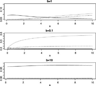
Figure 2: $\frac{F(a,b,\tilde{\ell}^{\star}(a,b))-F(a,b,\tilde{\ell}^{\alpha}(a,b))}{F(a,b,\tilde{\ell}^{\star}(a,b))}$ as function of $a$ for $b=1,0.1,10$ and $\alpha\simeq 0.27$ (solid line), $\alpha\simeq 0.35$ (dashed line), $\alpha=\mathrm{e}^{-1}\simeq 0.37$ (dotted line).

5.2 Gaussian case

Let us first consider the Gaussian target $V(x)=\frac{1}{2}(x^{2}+\ln(2\uppi))$ (see Remark 3), with a Gaussian initial condition $X_{0}$ such that $m(0)=\mathbb{E}(X_{0})$ and $s(0)=\mathbb{E}(X_{0}^{2})$. At time $t$, the law of $X_{t}$ solution to the limiting stochastic differential equation (1) is Gaussian with mean $m(t)$ and second moment $s(t)$, where $m$ and $s$ satisfies (30). The Kullback–Leibler divergence admits an analytical expression in terms of $m$ and $s$:

$$H(\psi_{t}|\psi_{\infty})={\textstyle\frac{1}{2}}\bigl{(}s(t)-\ln\bigl{(}s(t)-m(t)^{2}\bigr{)}-1\bigr{)},$$

and its derivative writes

$$\frac{\mathrm{d}}{\mathrm{d}t}H(\psi_{t}|\psi_{\infty}) = \frac{1}{2}\biggl{(}\frac{\mathrm{d}s}{\mathrm{d}t}-\frac{{\mathrm{d}s}/{\mathrm{d}t}-2m{\mathrm{d}m}/{\mathrm{d}t}}{s-m^{2}}\biggr{)}$$

$$= \frac{1}{2}\biggl{(}F_{1}(s,\ell)(1-s)-\frac{F_{1}(s,\ell)(1-s)+2m{\mathcal{G}}(s,1,\ell)}{s-m^{2}}\biggr{)}.$$

In the Gaussian case, it is thus possible, for each time $t$ (and thus for fixed values of $m(t)$ and $s(t)$), to minimize $\frac{\mathrm{d}}{\mathrm{d}t}H(\psi_{t}|\psi_{\infty})$ in $\ell$. This yields the best strategy that we could think of and implement numerically, in terms of the speed of convergence of the Kullback–Leibler divergence to 0. In the following, let us denote

$$\ell^{\mathrm{ent}}(m,s)=\arg\min_{\ell}\biggl{(}F_{1}(s,\ell)(1-s)-\frac{F_{1}(s,\ell)(1-s)+2m{\mathcal{G}}(s,1,\ell)}{s-m^{2}}\biggr{)}.$$

In the numerical experiments, we thus compare four strategies: (i) the constant $\ell$ strategy, with $\ell=2.38$ (which is the optimal value under stationarity assumption since $I=1$ in the Gaussian case); (ii) the constant average acceptance rate strategy, using $\ell^{\alpha}(a,b)$ (for $\alpha\simeq 0.27$ and $\alpha=\mathrm{e}^{-1}\simeq 0.37$); (iii) the optimal exponential rate of convergence using $\ell^{\star}(a,b)$; (iv) the optimal strategy for the convergence of the entropy using $\ell^{\mathrm{ent}}(m,s)$. Notice that in the Gaussian case, $a=\mathbb{E}(X_{t}^{2})=s(t)$ and $b=1$, so that $\ell^{\alpha}$ and $\ell^{\star}$ are actually functions of $s$ only. Let us also mention that there are actually two ways to implement (ii): either using a numerical approximation for $\ell^{\alpha}(a,1)$ (and an estimator $\hat{a}$ of $a$), or using the adaptive scaling Metropolis algorithm mentioned at the beginning of Section 4.2 (see [1, 3]).

The dimension is fixed to $n=100$. To assess the convergence, we observe, as a function of the so-called burn-in time $t_{0}$, the convergence to zero of the square biases:

$$\bigl{(}\mathbb{E}\bigl{(}\hat{I}^{s}_{t_{0},T+t_{0}}\bigr{)}-1\bigr{)}^{2}\quad\mbox{and}\quad\bigl{(}\mathbb{E}\bigl{(}\hat{I}^{m}_{t_{0},T+t_{0}}\bigr{)}\bigr{)}^{2},$$ (48)

where

$$\hat{I}^{s}_{t_{0},T+t_{0}}=\frac{1}{T}\sum_{k=t_{0}+1}^{T+t_{0}}\frac{(X_{k}^{1})^{2}+\cdots+(X_{k}^{100})^{2}}{100}$$ (49)

and

$$\hat{I}^{m}_{t_{0},T+t_{0}}=\frac{1}{T}\sum_{k=t_{0}+1}^{T+t_{0}}\frac{X_{k}^{1}+\cdots+X_{k}^{100}}{100}.$$ (50)

The expectations in (48) are approximated by empirical averages over 200 independent realizations of $(X_{k}^{1},\ldots,X_{k}^{100})_{0\leq k\leq t_{0}+T}$. The size of the time window is $T=1500$. When needed, we estimate the values of $s=a$ and $m$ using empirical averages over the $n=100$ components of the process.

On Figure 3, we first consider the initial condition $X_{0}=(0,\ldots,0)$. The first moment is thus already at equilibrium, and we only observe the convergence of the second moment. Clearly, the constant $\ell$ strategy is the worst. Using $\ell^{\star}$ yields a convergence which is almost the optimal one, obtained for $\ell=\ell^{\mathrm{ent}}$. And the constant average rate strategies also lead to excellent results in terms of convergence compared to the optimal scenario, even though it is here implemented using an adaptive scaling Metropolis algorithm.

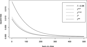
Figure 3: Square bias of $\hat{I}^{s}_{t_{0},t_{0}+T}$ as a function of the burn-in-time $t_{0}$ for various strategies. The initial condition is $(0,\ldots,0)$, and the constant acceptance rate strategies are implemented using an adaptive scaling Metropolis algorithm.

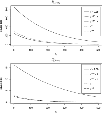
Figure 4: Square bias of $\hat{I}^{s}_{t_{0},T+t_{0}}$ (top) and $\hat{I}^{m}_{t_{0},T+t_{0}}$ (bottom) as a function of the burn-in-time $t_{0}$ for various strategies. The initial condition is $(10,\ldots,10)$. The notations $\ell^{0.27}-A$ and $\ell^{0.27}-N$ refer to the two implementations of the constant average acceptance rate: $A$ for the adaptive scaling Metropolis algorithm and $N$ for the numerical approximation of $\ell^{\alpha}(a,1)$.

On Figure 4, we perform similar experiments with the initial condition $X_{0}=(10,\ldots,10)$. We observe the convergence of the first and second moment. It is clear that the constant $\ell$ strategy is outperformed by all the other strategies. We notice also that the adaptive scaling Metropolis implementation leads to slightly slower convergences compared to an implementation using $\ell^{\alpha}(\hat{a},1)$. This difference could certainly be reduced by optimizing the parameters in the adaptive scaling Metropolis algorithm.

In conclusion, we observed that: (i) The constant $\ell$ strategy is bad; (ii) The constant average acceptance rate strategy (using $\ell^{\alpha}$) leads to convergence curves which are very close to the ones obtained with the optimal exponential rate of convergence strategy (using $\ell^{\star}$); (iii) the optimal exponential rate of convergence strategy is as good as the most optimal strategy one could design in terms of entropy decay (using $\ell^{\mathrm{ent}}$).

5.3 Non-Gaussian case

Let us now consider a non-Gaussian target, and more precisely a double-well potential. In order to satisfy the assumptions of Theorem 1, we consider the function $V$ given up to a normalizing additive constant by:

$$V(x)=\cases{(x-1)^{2}(x+1)^{2},&\quad\mbox{if } $|x|\leq 1$,\cr 4x^{2}-8|x|+4,&\quad\mbox{otherwise}.}$$

Simple calculations yield

$$V^{\prime}(x)=\cases{2(x-1)(x+1)^{2}+2(x-1)^{2}(x+1),&\quad\mbox{if } $|x|\leq 1$,\cr 8x-8\operatorname{sign}(x),&\quad\mbox{otherwise},}$$

and

$$V^{\prime\prime}(x)=\cases{2(x+1)^{2}+8(x-1)(x+1)+2(x-1)^{2},&\quad\mbox{if } $|x|\leq 1$,\cr 8,&\quad\mbox{otherwise}.}$$

Of course, no analytical expression for the entropy is available in this context, and we thus concentrate on the three following strategies: (i) the constant $\ell$ strategy; (ii) $\ell=\ell^{\alpha}(a,b)$ and (iii) $\ell=\ell^{\star}(a,b)$. For the constant $\ell$ strategy, we use $\ell=\frac{2.38}{\sqrt{I}}=1.18$ (where we recall, $I$ is defined by (4)). When needed, $a$ and $b$ are approximated by the estimators over the $n$ components $\hat{a}=\frac{1}{n}\sum_{i=1}^{n}V^{\prime}(X_{t}^{i})^{2}$ and $\hat{b}=\frac{1}{n}\sum_{i=1}^{n}V^{\prime\prime}(X_{t}^{i})$. The parameters $n=100$ and $T=1500$ are the same as in the Gaussian case.

Let us first consider as an initial condition $X_{0}=(10,\ldots,10)$. On Figure 5, we observe the convergence of the first moment to its equilibrium value (namely 0). Again, the constant $\ell$ strategy appears to be very bad, and the other strategies perform approximately equally well.

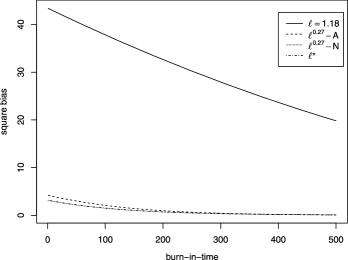
Figure 5: Square bias of $\hat{I}^{m}_{t_{0},T+t_{0}}$ for non-Gaussian target as a function of the burn-in-time $t_{0}$ for various strategies. The initial condition is $(10,\ldots,10)$. The notations $\ell^{0.27}-A$ and $\ell^{0.27}-N$ refer to the two implementations of the constant average acceptance rate: $A$ for the adaptive scaling Metropolis algorithm and $N$ for the numerical approximation of $\ell^{\alpha}(a,b)$.

Finally, let us consider $X_{0}$ distributed according to a Gaussian distribution with mean $1$ and variance $0.143\mathrm{Id}$. The mean and the variance are chosen in such a way that $a=\mathbb{E}(V^{\prime}(X_{0})^{2})=5.24$ and $b=\mathbb{E}(V^{\prime\prime}(X_{0}))=5.24$. On Figure 6, we observe the convergence of the first and second moments to their equilibrium values (namely 0 and 0.96). For the constant acceptance rate strategy, we compare the results obtained with $\alpha=0.35$ and $\alpha=0.27$. Here, it is much more complicated to draw general conclusions from these plots. Basically, all strategies yield comparable results. One could wonder why $\ell^{\star}$ performs poorly for the first moment. The reason is probably that its bias cannot be encoded into $a$ and $b$ which are integrals of even functions with respect to the current marginal distribution.

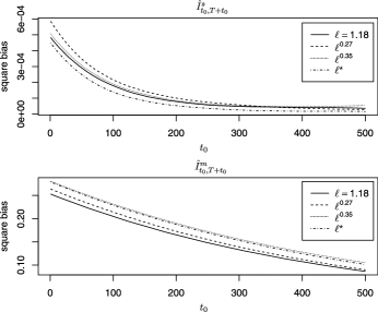
Figure 6: Square bias of $\hat{I}^{s}_{t_{0},T+t_{0}}$ (top) and $\hat{I}^{m}_{t_{0},T+t_{0}}$ (bottom) for non-Gaussian target as a function of the burn-in-time $t_{0}$ for various strategies and Gaussian initial condition. The constant acceptance rate strategies are implemented using an adaptive scaling Metropolis algorithm.

In conclusion, we observed that the results obtained with the constant acceptance rate strategy (even when it is implemented using an adaptive scaling Metropolis algorithm) are very similar to those obtained with the optimal exponential rate of convergence strategy.

6 Scaling limits for the MALA algorithm

The aim of this section is to derive a diffusive limit for the MALA algorithm, following the same reasoning as for the RWM algorithm in Section 2.

The Markov chain generated by the MALA algorithm writes:

$$X^{i,n}_{k+1}=X^{i,n}_{k}+Z^{i,n}_{k+1}1_{{\mathcal{A}}_{k+1}}$$ (51)

$$\quad\mbox{where }Z^{i,n}_{k+1}=\sigma_{n}G^{i}_{k+1}-\frac{\sigma_{n}^{2}}{2}V^{\prime}\bigl{(}X^{i,n}_{k}\bigr{)},\qquad 1\leq i\leq n,$$

$$\quad\mbox{and }{\mathcal{A}}_{k+1}=\Biggl{\{}U_{k+1}\leq\exp\Biggl{\{}\sum_{i=1}^{n}\biggl{(}V\bigl{(}X^{i,n}_{k}\bigr{)}-V\bigl{(}X^{i,n}_{k}+Z^{i,n}_{k+1}\bigr{)}$$

$$\hphantom{\quad\mbox{and }{\mathcal{A}}_{k+1}=\Biggl{\{}}{}+\frac{1}{2}\biggl{[}\bigl{(}G^{i}_{k+1}\bigr{)}^{2}-\biggl{(}G^{i}_{k+1}-\frac{\sigma_{n}}{2}\bigl{(}V^{\prime}\bigl{(}X^{i,n}_{k}\bigr{)}+V^{\prime}\bigl{(}X^{i,n}_{k}+Z^{i,n}_{k+1}\bigr{)}\bigr{)}\biggr{)}^{2}\biggr{]}\biggr{)}\Biggr{\}}\Biggr{\}}$$

is the accepting event. Here again, $(G^{i}_{k})_{i,k\geq 1}$ is a sequence of i.i.d. normal random variables independent from a sequence $(U_{k})_{k\geq 1}$ of i.i.d. random variables uniform on $[0,1]$. In Section 6.1, we formally derive a limiting diffusion process. It appears that the scaling to be used depend on the sign of $\mathbb{E}(((V^{\prime})^{2}V^{\prime\prime}+V^{(4)}-2V^{(3)}V^{\prime}-(V^{\prime\prime})^{2})(X^{1,n}_{k}))$. This is more rigorously discussed in Section 6.2 for a Gaussian target probability measure.

6.1 A formal derivation of the limiting process

6.1.1 Asymptotic analysis and limiting process

We adapt the same strategy as for the RWM algorithm, in Section 2.2. Let us first discuss how to choose the proper scaling for $\sigma_{n}$. Using a Taylor expansion, one obtains:

$$V\bigl{(}X^{i,n}_{k}\bigr{)}-V\bigl{(}X^{i,n}_{k}+Z^{i,n}_{k+1}\bigr{)}+\frac{1}{2}\biggl{[}\bigl{(}G^{i}_{k+1}\bigr{)}^{2}-\biggl{(}G^{i}_{k+1}-\frac{\sigma_{n}}{2}\bigl{(}V^{\prime}\bigl{(}X^{i,n}_{k}\bigr{)}+V^{\prime}\bigl{(}X^{i,n}_{k}+Z^{i,n}_{k+1}\bigr{)}\bigr{)}\biggr{)}^{2}\biggr{]}$$

$$\quad=\sigma_{n}^{3}\biggl{(}\frac{V^{(3)}(X^{i,n}_{k})}{12}\bigl{(}G^{i}_{k+1}\bigr{)}^{3}-\frac{V^{\prime}V^{\prime\prime}(X^{i,n}_{k})}{4}G^{i}_{k+1}\biggr{)}$$

$$\qquad{}+\sigma_{n}^{4}\biggl{(}\frac{(V^{\prime})^{2}V^{\prime\prime}(X^{i,n}_{k})}{8}+\frac{V^{(4)}(X^{i,n}_{k})}{24}\bigl{(}G^{i}_{k+1}\bigr{)}^{4}-\frac{2V^{(3)}V^{\prime}(X^{i,n}_{k})+(V^{\prime\prime}(X^{i,n}_{k}))^{2}}{8}\bigl{(}G^{i}_{k+1}\bigr{)}^{2}\biggr{)}$$

$$\qquad{}+{\mathcal{\mathcal{O}}}\bigl{(}\sigma_{n}^{5}\bigr{)}.$$

Setting, as above, $\nu^{n}_{k}=\frac{1}{n}\sum_{i=1}^{n}\delta_{X^{i,n}_{k}}$, one has by Gaussian computations

$$\mathbb{E}\Biggl{(}\Biggl{(}\sum_{i=1}^{n}\biggl{(}\frac{V^{(3)}(X^{i,n}_{k})}{12}\bigl{(}G^{i}_{k+1}\bigr{)}^{3}-\frac{V^{\prime}V^{\prime\prime}(X^{i,n}_{k})}{4}G^{i}_{k+1}\biggr{)}\Biggr{)}^{2}\Biggr{)}$$

$$\quad=\frac{n}{48}\mathbb{E}\bigl{(}\bigl{\langle}\nu^{n}_{k},5\bigl{(}V^{(3)}\bigr{)}^{2}-6V^{\prime}V^{\prime\prime}V^{(3)}+3\bigl{(}V^{\prime}V^{\prime\prime}\bigr{)}^{2}\bigr{\rangle}\bigr{)}$$

so that one expects that $\sum_{i=1}^{n}(\frac{V^{(3)}(X^{i,n}_{k})}{12}(G^{i}_{k+1})^{3}-\frac{V^{\prime}V^{\prime\prime}(X^{i,n}_{k})}{4}G^{i}_{k+1})={\mathcal{O}}(\sqrt{n})$ and similarly that $\sum_{i=1}^{n}(\frac{V^{(4)}(X^{i,n}_{k})}{24}((G^{i}_{k+1})^{4}-3)-\frac{2V^{(3)}V^{\prime}(X^{i,n}_{k})+(V^{\prime\prime}(X^{i,n}_{k}))^{2}}{8}((G^{i}_{k+1})^{2}-1))={\mathcal{O}}(\sqrt{n})$. If this holds and $\lim_{n\to\infty}\sigma_{n}=0$, then

$$\sum_{i=1}^{n}\biggl{(}V\bigl{(}X^{i,n}_{k}\bigr{)}-V\bigl{(}X^{i,n}_{k}+Z^{i,n}_{k+1}\bigr{)}$$

$$\hphantom{\sum_{i=1}^{n}\biggl{(}}{}+\frac{1}{2}\biggl{[}\bigl{(}G^{i}_{k+1}\bigr{)}^{2}-\biggl{(}G^{i}_{k+1}-\frac{\sigma_{n}}{2}\bigl{(}V^{\prime}\bigl{(}X^{i,n}_{k}\bigr{)}+V^{\prime}\bigl{(}X^{i,n}_{k}+Z^{i,n}_{k+1}\bigr{)}\bigr{)}\biggr{)}^{2}\biggr{]}\biggr{)}$$

$$\quad=\frac{n\sigma_{n}^{4}}{8}\bigl{\langle}\nu^{n}_{k},\bigl{(}V^{\prime}\bigr{)}^{2}V^{\prime\prime}+V^{(4)}-2V^{(3)}V^{\prime}-\bigl{(}V^{\prime\prime}\bigr{)}^{2}\bigr{\rangle}+{\mathcal{O}}\bigl{(}\sqrt{n}\sigma_{n}^{3}\bigr{)}+{\mathcal{O}}\bigl{(}n\sigma_{n}^{5}\bigr{)}.$$

From this,

$$\mathbb{E}\bigl{(}1_{{\mathcal{A}}_{k+1}}|{\mathcal{F}}^{n}_{k}\bigr{)}=\mathrm{e}^{({n\sigma_{n}^{4}}/{8})\langle\nu^{n}_{k},((V^{\prime})^{2}V^{\prime\prime}+V^{(4)}-2V^{(3)}V^{\prime}-(V^{\prime\prime})^{2})\rangle}\wedge 1+{\mathcal{O}}\bigl{(}\sqrt{n}\sigma_{n}^{3}\bigr{)}+{\mathcal{O}}\bigl{(}n\sigma_{n}^{5}\bigr{)}.$$ (52)

Here, we have assumed that $\langle\nu^{n}_{k},(V^{\prime})^{2}V^{\prime\prime}+V^{(4)}-2V^{(3)}V^{\prime}-(V^{\prime\prime})^{2}\rangle\neq 0$. From this formula, we get the correct scaling for the variance, in order to obtain a nontrivial limiting acceptance rate (in accordance with [12], Section 5):

$$\sigma_{n}^{4}=\frac{\ell^{4}}{n}.$$

Now, following the same reasoning as in Section 2.2, we have: for a test function $\varphi\mathchoice{\nobreak\,\colon}{\nobreak\,\colon}{\nobreak\,\colon\;}{\nobreak\,\colon\;}\mathbb{R}\to\mathbb{R}$,

$$\mathbb{E}\bigl{(}\varphi\bigl{(}X^{1,n}_{k+1}\bigr{)}|{\mathcal{F}}^{n}_{k}\bigr{)}$$

$$\quad=\mathbb{E}\bigl{(}\varphi\bigl{(}X^{1,n}_{k}+Z^{1,n}_{k+1}1_{{\mathcal{A}}_{k+1}}\bigr{)}|{\mathcal{F}}^{n}_{k}\bigr{)}$$

$$\quad=\mathbb{E}\biggl{(}\varphi\bigl{(}X^{1,n}_{k}\bigr{)}+\varphi^{\prime}\bigl{(}X^{1,n}_{k}\bigr{)}Z^{1,n}_{k+1}1_{{\mathcal{A}}_{k+1}}+{\textstyle\frac{1}{2}}\varphi^{\prime\prime}\bigl{(}X^{1,n}_{k}\bigr{)}\bigl{(}Z^{1,n}_{k+1}\bigr{)}^{2}1_{{\mathcal{A}}_{k+1}}|{\mathcal{F}}^{n}_{k}\biggr{)}+{\mathcal{O}}\bigl{(}n^{-3/4}\bigr{)}$$

$$\quad=\varphi\bigl{(}X^{1,n}_{k}\bigr{)}+\varphi^{\prime}\bigl{(}X^{1,n}_{k}\bigr{)}\mathbb{E}\bigl{(}Z^{1,n}_{k+1}1_{{\mathcal{A}}_{k+1}}|{\mathcal{F}}^{n}_{k}\bigr{)}+{\textstyle\frac{1}{2}}\varphi^{\prime\prime}\bigl{(}X^{1,n}_{k}\bigr{)}\mathbb{E}\bigl{(}\bigl{(}Z^{1,n}_{k+1}\bigr{)}^{2}1_{{\mathcal{A}}_{k+1}}|{\mathcal{F}}^{n}_{k}\bigr{)}+{\mathcal{O}}\bigl{(}n^{-3/4}\bigr{)}.$$

Using the Lipschitz continuity of $y\mapsto\mathrm{e}^{y}\wedge 1$, one may remove the contribution of the $i$th coordinate in the acceptance ratio and then introduce it again after using conditional independence to check that

$$\mathbb{E}\bigl{(}G^{i}_{k+1}1_{{\mathcal{A}}_{k+1}}|{\mathcal{F}}^{n}_{k}\bigr{)} = \mathbb{E}\bigl{(}G^{i}_{k+1}\bigr{)}\mathbb{E}\bigl{(}1_{{\mathcal{A}}_{k+1}}|{\mathcal{F}}^{n}_{k}\bigr{)}+{\mathcal{O}}\bigl{(}\sigma_{n}^{3}\bigr{)}={\mathcal{O}}\bigl{(}n^{-3/4}\bigr{)},$$

$$\mathbb{E}\bigl{(}\bigl{(}G^{i}_{k+1}\bigr{)}^{2}1_{{\mathcal{A}}_{k+1}}|{\mathcal{F}}^{n}_{k}\bigr{)} = \mathbb{E}\bigl{[}\bigl{(}G^{i}_{k+1}\bigr{)}^{2}\bigr{]}\mathbb{E}\bigl{(}1_{{\mathcal{A}}_{k+1}}|{\mathcal{F}}^{n}_{k}\bigr{)}+{\mathcal{O}}\bigl{(}\sigma_{n}^{3}\bigr{)}=\mathbb{P}\bigl{(}{\mathcal{A}}_{k+1}|{\mathcal{F}}^{n}_{k}\bigr{)}+{\mathcal{O}}\bigl{(}n^{-3/4}\bigr{)}.$$

From this, one obtains

$$\mathbb{E}\bigl{(}\varphi\bigl{(}X^{1,n}_{k+1}\bigr{)}|{\mathcal{F}}^{n}_{k}\bigr{)}$$

$$\quad=\varphi\bigl{(}X^{1,n}_{k}\bigr{)}+\varphi^{\prime}\bigl{(}X^{1,n}_{k}\bigr{)}\mathbb{E}\biggl{(}\biggl{(}\sigma_{n}G^{i}_{k+1}-\frac{\sigma_{n}^{2}}{2}V^{\prime}\bigl{(}X^{1,n}_{k}\bigr{)}\biggr{)}1_{{\mathcal{A}}_{k+1}}\big{|}{\mathcal{F}}^{n}_{k}\biggr{)}$$

$$\qquad{}+\frac{1}{2}\varphi^{\prime\prime}\bigl{(}X^{1,n}_{k}\bigr{)}\mathbb{E}\biggl{(}\biggl{(}\sigma_{n}G^{i}_{k+1}-\frac{\sigma_{n}^{2}}{2}V^{\prime}\bigl{(}X^{1,n}_{k}\bigr{)}\biggr{)}^{2}1_{{\mathcal{A}}_{k+1}}\big{|}{\mathcal{F}}^{n}_{k}\biggr{)}+{\mathcal{O}}\bigl{(}n^{-3/4}\bigr{)}$$

$$\quad=\varphi\bigl{(}X^{1,n}_{k}\bigr{)}+\frac{\ell^{2}}{2\sqrt{n}}\bigl{(}\mathrm{e}^{({\ell^{4}}/{8})\langle\nu^{n}_{k},((V^{\prime})^{2}V^{\prime\prime}+V^{(4)}-2V^{(3)}V^{\prime}-(V^{\prime\prime})^{2})\rangle}\wedge 1\bigr{)}$$

$$\qquad{}\times\bigl{(}-V^{\prime}\bigl{(}X^{1,n}_{k}\bigr{)}\varphi^{\prime}\bigl{(}X^{1,n}_{k}\bigr{)}+\varphi^{\prime\prime}\bigl{(}X^{1,n}_{k}\bigr{)}\bigr{)}+{\mathcal{O}}\bigl{(}n^{-3/4}\bigr{)}.$$

The correct scaling in time is thus to consider a piecewise linear process $Y^{1,n}_{t}$ such that $Y^{1,n}_{k/\sqrt{n}}=X^{1,n}_{k}$ (this is again the standard diffusive timescale), and the expected propagation of chaos limit is solution to the nonlinear stochastic differential equation:

$$\mathrm{d}X_{t}=\sqrt{w(t,\ell)}\,\mathrm{d}B_{t}-w(t,\ell){\textstyle\frac{1}{2}}V^{\prime}(X_{t})\,\mathrm{d}t,$$

(53)

$$\quad\mbox{where }w(t,\ell)=\ell^{2}\bigl{(}\mathrm{e}^{({\ell^{4}}/{8})\mathbb{E}(((V^{\prime})^{2}V^{\prime\prime}+V^{(4)}-2V^{(3)}V^{\prime}-(V^{\prime\prime})^{2})(X_{t}))}\wedge 1\bigr{)}.$$

This equation is obtained by a deterministic (and nonlinear in the sense of McKean) change of time applied to the standard overdamped Langevin stochastic differential equation with reversible density $\mathrm{e}^{-V}$. Under appropriate assumptions on the potential $V$, we believe that a rigorous proof of this result could be done using similar techniques as for the RWM algorithm in [14].

6.1.2 Relation to previous results in the literature

These results are related to previous ones in the literature. First, in the Gaussian case $V(x)=\frac{x^{2}}{2}+\frac{1}{2}\ln(2\uppi)$, one obtains from (6.1.1) that $(\mathbb{E}(X_{t}^{2}))_{t\geq 0}$ solves the ordinary differential equation

$$\frac{\mathrm{d}}{\mathrm{d}t}\mathbb{E}\bigl{(}X_{t}^{2}\bigr{)}=\ell^{2}\bigl{(}\mathrm{e}^{({\ell^{4}}/{8})(\mathbb{E}(X_{t}^{2})-1)}\wedge 1\bigr{)}\bigl{(}1-\mathbb{E}\bigl{(}X_{t}^{2}\bigr{)}\bigr{)}.$$

We recover here a result from [12], Theorem 2, where it is shown that the process $(\frac{1}{n}\sum_{i=1}^{n}(X^{i,n}_{\lfloor\sqrt{n}t\rfloor})^{2})_{t\geq 0}$, in the limit $n\to\infty$ satisfies this ordinary differential equation.

Second, in the stationary case, namely when $(X^{1,n}_{0},\ldots,X^{n,n}_{0})$ are distributed according to the target density $p$ defined by (2), the equalities

$$\int_{\mathbb{R}}V^{(3)}V^{\prime}(x)\mathrm{e}^{-V(x)}\,\mathrm{d}x = \int_{\mathbb{R}}V^{(4)}(x)\mathrm{e}^{-V(x)}\,\mathrm{d}x,$$

$$\int_{\mathbb{R}}V^{\prime\prime}\bigl{(}V^{\prime}\bigr{)}^{2}(x)\mathrm{e}^{-V(x)}\,\mathrm{d}x = \int_{\mathbb{R}}\bigl{[}V^{(3)}V^{\prime}+\bigl{(}V^{\prime\prime}\bigr{)}^{2}\bigr{]}(x)\mathrm{e}^{-V(x)}\,\mathrm{d}x$$

imply that $\langle\nu^{n}_{k},((V^{\prime})^{2}V^{\prime\prime}+V^{(4)}-2V^{(3)}V^{\prime}-(V^{\prime\prime})^{2})\rangle=0$ and this changes the scaling of the limiting acceptance rate in (52). In [23], it is shown that in this case, the correct scaling is $\sigma_{n}^{2}=\frac{\ell^{2}}{n^{1/3}}$ and then $(X^{1,n}_{\lfloor n^{1/3}t\rfloor})_{t\geq 0}$ converges in distribution to the solution $(X_{t})_{t\geq 0}$ of the stochastic differential equation

$$\mathrm{d}X_{t}=\sqrt{z(\ell)}\,\mathrm{d}B_{t}-z(\ell)\frac{1}{2}V^{\prime}(X_{t})\,\mathrm{d}t,$$

(54)

$$\quad\mbox{where }z(\ell)=2\ell^{2}\Phi\biggl{(}-\frac{\ell^{3}\sqrt{\langle m,5(V^{(3)})^{2}-3(V^{\prime\prime})^{3}\rangle/3}}{8}\biggr{)},$$

where $\mathrm{d}m=\mathrm{e}^{-V(x)}\,\mathrm{d}x$.

6.1.3 Practical counterparts

The practical counterparts of the convergence results discussed above are the following. We can actually distinguish between three regimes:

• [$\bullet$]

• On time intervals such that $\mathbb{E}(((V^{\prime})^{2}V^{\prime\prime}+V^{(4)}-2V^{(3)}V^{\prime}-(V^{\prime\prime})^{2})(X^{1,n}_{k}))<0$, then the correct scaling to obtain a diffusive limit is $\sigma_{n}^{2}=\frac{\ell^{2}}{n^{1/2}}$ and there exists an optimal value of $\ell$ to speed up the time scale of the dynamics of $X_{t}$, by maximizing $w(t,\ell)$ (see Equation (6.1.1)).

• On time intervals such that $\mathbb{E}(((V^{\prime})^{2}V^{\prime\prime}+V^{(4)}-2V^{(3)}V^{\prime}-(V^{\prime\prime})^{2})(X^{1,n}_{k}))=0$, then the correct scaling to obtain a diffusive limit is $\sigma_{n}^{2}=\frac{\ell^{2}}{n^{1/3}}$, and again, there exists on optimal value of $\ell$ to speed up the convergence to equilibrium, by maximizing $z(\ell)$ (see Equation (6.1.2) and [23]).

• On time intervals such that $\mathbb{E}(((V^{\prime})^{2}V^{\prime\prime}+V^{(4)}-2V^{(3)}V^{\prime}-(V^{\prime\prime})^{2})(X^{1,n}_{k}))>0$, with the scaling $\sigma_{n}^{2}=\frac{\ell^{2}}{n^{1/2}}$, we observe that $w(t,\ell)=\ell^{2}$ in (6.1.1) so that one should take $\ell$ as large as possible. This is an indication of the fact that the correct scaling for $\sigma_{n}^{2}$ in this case should be such that $\sigma_{n}^{2}\gg\frac{\ell^{2}}{n^{1/2}}$. Indeed, in the Gaussian case, Proposition 4 below shows that one should take $\sigma_{n}$ going to $0$ as slowly as possible.

In conclusion, in the MALA case (and contrary to the RWM case), the correct scaling as a function of the dimension is not the same at equilibrium and in the transient phase. Moreover, in the transient phase, the scaling depends on the sign of

$$\mathbb{E}\bigl{(}\bigl{(}\bigl{(}V^{\prime}\bigr{)}^{2}V^{\prime\prime}+V^{(4)}-2V^{(3)}V^{\prime}-\bigl{(}V^{\prime\prime}\bigr{)}^{2}\bigr{)}\bigl{(}X^{1,n}_{k}\bigr{)}\bigr{)}.$$

It seems thus difficult to draw any general simple recommendation for practitioners from this analysis. It is likely that the assumption that the target probability is the product of $n$ one-dimensional laws is too restrictive to understand correctly the scaling $n\to\infty$ in this case.

6.2 Rigorous results in the Gaussian case and when $\mathbb{E}((X^{1,n}_{k})^{2})>1$

In this section, we consider the case of a Gaussian target, namely

$$V(x)=\frac{x^{2}}{2}+\frac{1}{2}\ln(2\uppi).$$ (55)

We thus have

$$\bigl{(}V^{\prime}\bigr{)}^{2}V^{\prime\prime}+V^{(4)}-2V^{(3)}V^{\prime}-\bigl{(}V^{\prime\prime}\bigr{)}^{2}=x^{2}-1.$$

The aim of this section is to study in details the situation when

$$\mathbb{E}\bigl{(}\bigl{(}\bigl{(}V^{\prime}\bigr{)}^{2}V^{\prime\prime}+V^{(4)}-2V^{(3)}V^{\prime}-\bigl{(}V^{\prime\prime}\bigr{)}^{2}\bigr{)}\bigl{(}X^{1,n}_{k}\bigr{)}\bigr{)}>0\quad\mbox{namely}\quad\mathbb{E}\bigl{(}\bigl{(}X^{1,n}_{k}\bigr{)}^{2}\bigr{)}>1.$$

Proposition 3.

Let us consider $(X_{k}^{i,n})$ solution to (51) for the Gaussian target (55), with a variance independent of $n$:

$$\sigma_{n}=\ell\in(0,2).$$

Let $m$ be a probability measure on $\mathbb{R}$ such that $\langle m,x^{2}\rangle>\frac{1}{1-\ell^{2}/4}$. We endow the space $\mathbb{R}^{\mathbb{N}}$ with the product topology. If the initial random variables $(X^{1,n}_{0},\ldots,X^{n,n}_{0})$ are exchangeable and $m$-chaotic, then the processes $(X^{1,n},\ldots,X^{n,n})$ are $P$-chaotic where $P$ denotes the law of the Markov chain

$$Y_{k+1}=\biggl{(}1-\frac{\ell^{2}}{2}\biggr{)}Y_{k}+\ell G_{k+1}$$ (56)

with the sequence $(G_{k})$ i.i.d. according to the normal law and independent from the initial position $Y_{0}$ distributed according to $m$.

A simple case for which the assumption on the initial condition is satisfied is i.i.d. initial conditions $(X^{i,n}_{0})_{i}$ with law $m$.

Notice that $Y_{k}$ converges in law to ${\mathcal{N}}(0,\frac{1}{1-\ell^{2}/4})$ as $k\to+\infty$. The asymptotic distribution converges to the target density when $\ell\to 0$. Of course, for fixed $n$ and $i\in\{1,\ldots,n\}$, $X^{i,n}_{k}$ converges in law to ${\mathcal{N}}(0,1)$ as $k\to+\infty$. So the limits $k\to\infty$ and $n\to\infty$ do not commute, meaning that, for large $n$, the rate of convergence in distribution of $(X^{i,n}_{k})_{k\geq 1}$ to ${\mathcal{N}}(0,1)$ should deteriorate.

Proof of Proposition 3 Let $(Y^{1,n},\ldots,Y^{n,n})$ with $Y^{i,n}_{0}=X^{i,n}_{0}$ and $Y^{i,n}_{k+1}=(1-\frac{\ell^{2}}{2})Y^{i,n}_{k}+\ell G^{i}_{k+1}$ denote the processes obtained when all moves are accepted in the MALA algorithm (51). The proof is divided into two steps. We are first going to prove that the processes $(Y^{1,n},\ldots,Y^{n,n})$ are $P$-chaotic (this would be trivial if the initial conditions $(X^{i,n}_{0})_{i}$ were supposed to be i.i.d.). Then, setting

$$\tilde{\mathcal{A}}^{n}_{k+1}=\Biggl{\{}U_{k+1}\leq\exp\Biggl{\{}\sum_{i=1}^{n}\biggl{(}V\bigl{(}Y^{i,n}_{k}\bigr{)}-V\bigl{(}Y^{i,n}_{k+1}\bigr{)}$$

$$\hphantom{\tilde{\mathcal{A}}^{n}_{k+1}=\Biggl{\{}U_{k+1}\leq\exp\Biggl{\{}\sum_{i=1}^{n}\biggl{(}}{}+\frac{1}{2}\biggl{[}\bigl{(}G^{i}_{k+1}\bigr{)}^{2}-\biggl{(}G^{i}_{k+1}-\frac{\ell}{2}\bigl{(}V^{\prime}\bigl{(}Y^{i,n}_{k}\bigr{)}+V^{\prime}\bigl{(}Y^{i,n}_{k+1}\bigr{)}\bigr{)}\biggr{)}^{2}\biggr{]}\biggr{)}\Biggr{\}}\Biggr{\}},$$

we will check that $\forall K\in{\mathbb{N}}^{*},\lim_{n\to\infty}\mathbb{P}(\bigcap_{k=1}^{K}\tilde{\mathcal{A}}^{n}_{k})=1$. Since, on the event $\bigcap_{k=1}^{K}\tilde{\mathcal{A}}^{n}_{k}$, $(X^{1,n}_{k},\ldots,\allowbreak X^{n,n}_{k})_{0\leq k\leq K}=(Y^{1,n}_{k},\ldots,Y^{n,n}_{k})_{0\leq k\leq K}$ one obtains the $P$-chaoticity of the processes $(X^{1,n},\ldots,\allowbreak X^{n,n})$ by combining the two steps.

For the first step, notice that for fixed $j,K\in{\mathbb{N}}^{*}$, the law of $((Y^{1,n}_{k},\ldots,Y^{j,n}_{k}))_{0\leq k\leq K}$ is

$$m_{j}^{n}\bigl{(}\mathrm{d}y_{0}^{1},\ldots,\mathrm{d}y_{0}^{j}\bigr{)}\prod_{k=0}^{K-1}\bigl{(}Q\bigl{(}y^{1}_{k},\mathrm{d}y^{1}_{k+1}\bigr{)}\times\cdots\times Q\bigl{(}y^{j}_{k},\mathrm{d}y^{j}_{k+1}\bigr{)}\bigr{)},$$

where $Q(y,\mathrm{d}y^{\prime})=\frac{1}{\ell\sqrt{2\uppi}}\mathrm{e}^{-{(y^{\prime}-y(1-\ell^{2}/2))^{2}}/({2\ell^{2}})}\,\mathrm{d}y^{\prime}$ and the law $m^{n}_{j}$ of $(X^{1,n}_{0},\ldots,X^{j,n}_{0})$ converges weakly to $m^{\otimes j}$ as $n\to\infty$ (since the initial conditions $(X^{1,n}_{0},\ldots,X^{n,n}_{0})$ are $m$-chaotic). Since $y\mapsto Q(y,\mathrm{d}y^{\prime})\in{\mathcal{P}}(\mathbb{R})$ is weakly continuous, this law converges weakly to $\prod_{i=1}^{j}(m(\mathrm{d}y^{i}_{0})\prod_{k=0}^{K-1}Q(y^{i}_{k},\mathrm{d}y^{i}_{k+1}))$ which is the $j$-fold product of the image of $P$ by the canonical restriction to the $K+1$ first coordinates. Hence, the processes $(Y^{1,n},\ldots,Y^{n,n})$ are $P$-chaotic.

For the second step, let us introduce

$$S^{n}_{k}=\frac{8}{n\ell^{4}}\sum_{i=1}^{n}\biggl{\{}V\bigl{(}Y^{i,n}_{k}\bigr{)}-V\bigl{(}Y^{i,n}_{k+1}\bigr{)}+\frac{1}{2}\biggl{[}\bigl{(}G^{i}_{k+1}\bigr{)}^{2}-\biggl{(}G^{i}_{k+1}-\frac{\ell}{2}\bigl{(}V^{\prime}\bigl{(}Y^{i,n}_{k}\bigr{)}+V^{\prime}\bigl{(}Y^{i,n}_{k+1}\bigr{)}\bigr{)}\biggr{)}^{2}\biggr{]}\biggr{\}}.$$

One has

$$\mathbb{P}\bigl{(}\bigl{\{}\tilde{\mathcal{A}}^{n}_{k+1}\bigr{\}}^{c}\bigr{)}\leq\mathbb{P}\bigl{(}S^{n}_{k}<0\bigr{)}.$$ (57)

Some tedious but simple computations yields (using $V(x)=\frac{x^{2}}{2}+\frac{1}{2}\ln(2\uppi)$)

$$V\bigl{(}Y^{i,n}_{k}\bigr{)}-V\bigl{(}Y^{i,n}_{k+1}\bigr{)}+\frac{1}{2}\biggl{[}\bigl{(}G^{i}_{k+1}\bigr{)}^{2}-\biggl{(}G^{i}_{k+1}-\frac{\ell}{2}\bigl{(}V^{\prime}\bigl{(}Y^{i,n}_{k}\bigr{)}+V^{\prime}\bigl{(}Y^{i,n}_{k+1}\bigr{)}\bigr{)}\biggr{)}^{2}\biggr{]}$$

(58)

$$\quad=\frac{\ell^{4}}{8}\bigl{(}\bigl{(}Y^{i,n}_{k}\bigr{)}^{2}-\bigl{(}G^{i}_{k+1}\bigr{)}^{2}\bigr{)}+\biggl{(}\frac{\ell^{5}}{8}-\frac{\ell^{3}}{4}\biggr{)}Y^{i,n}_{k}G^{i}_{k+1}-\frac{\ell^{6}}{32}\bigl{(}Y^{i,n}_{k}\bigr{)}^{2}$$

so that (in law)

$$S_{k}^{n}=\biggl{(}1-\frac{\ell^{2}}{4}\biggr{)}\bigl{\langle}\mu^{n}_{k},y^{2}\bigr{\rangle}+\biggl{(}\ell-\frac{2}{\ell}\biggr{)}\sqrt{\bigl{\langle}\mu^{n}_{k},y^{2}\bigr{\rangle}}\frac{\tilde{G}^{n}_{k+1}}{\sqrt{n}}-\frac{1}{n}\sum_{i=1}^{n}\bigl{(}G^{i}_{k+1}\bigr{)}^{2}$$

with $\tilde{G}^{n}_{k+1}=1_{\{\langle\mu^{n}_{k},y^{2}\rangle>0\}}\frac{\sum_{i=1}^{n}Y^{i}_{k}G^{i}_{k+1}}{\sqrt{n\langle\mu^{n}_{k},y^{2}\rangle}}+1_{\{\langle\mu^{n}_{k},y^{2}\rangle=0\}}G^{1}_{k+1}$ a normal random variable independent from $\mu^{n}_{k}=\frac{1}{n}\sum_{i=1}^{n}\delta_{Y^{i,n}_{k}}$. As the exchangeability of the initial condition $(Y^{1,n}_{0},\ldots,Y^{n,n}_{0})$ is preserved by the evolution, the propagation of chaos result obtained in the first step implies (and is actually equivalent to) the convergence in probability of the empirical measures $\mu^{n}=\frac{1}{n}\sum_{i=1}^{n}\delta_{Y^{i,n}}\in{\mathcal{P}}(\mathbb{R}^{\mathbb{N}})$ to $P$ (see [25], Proposition 2.2). In particular, $\mu^{n}_{k}$ converges in probability to the law $P_{k}$ of $Y_{k}$, solution to (56).

With this law of large numbers, we see that in order to estimate $\mathbb{P}(S^{n}_{k}<0)$ we need to understand the evolution of $\langle P_{k},y^{2}\rangle=\mathbb{E}((Y_{k})^{2})$ with $k$. One has $\langle P_{k+1},y^{2}\rangle=(1-\frac{\ell^{2}}{2})^{2}\langle P_{k},y^{2}\rangle+\ell^{2}$, and since $\langle P_{0},y^{2}\rangle=\langle m,y^{2}\rangle>\frac{1}{1-\ell^{2}/4}$, one easily checks by induction that for all $k\in{\mathbb{N}}$, $\langle P_{k},y^{2}\rangle>\frac{1}{1-\ell^{2}/4}$. Hence for fixed $k\in{\mathbb{N}}$, there exists $M<+\infty$ and $\varepsilon>0$ such that $\langle P_{k},y^{2}\wedge M\rangle\geq\frac{1+3\varepsilon}{1-\ell^{2}/4}$. One has

$$\mathbb{P}\bigl{(}S^{n}_{k}<0\bigr{)} \leq \mathbb{P}\Biggl{(}\frac{1}{n}\sum_{i=1}^{n}\bigl{(}G^{i}_{k+1}\bigr{)}^{2}>1+\varepsilon\Biggr{)}$$

$${}+\mathbb{P}\biggl{(}\bigl{\langle}\mu^{n}_{k},y^{2}\bigr{\rangle}\biggl{(}1+\frac{\ell-2/\ell}{1-\ell^{2}/4}\frac{\tilde{G}^{n}_{k+1}}{\sqrt{n\langle\mu^{n}_{k},y^{2}\rangle}}\biggr{)}<\frac{1+\varepsilon}{1-\ell^{2}/4}\biggr{)}$$

$$\leq \mathbb{P}\Biggl{(}\frac{1}{n}\sum_{i=1}^{n}\bigl{(}G^{i}_{k+1}\bigr{)}^{2}>1+\varepsilon\Biggr{)}+\mathbb{P}\biggl{(}\bigl{\langle}\mu^{n}_{k},y^{2}\wedge M\bigr{\rangle}<\frac{1+2\varepsilon}{1-\ell^{2}/4}\biggr{)}$$

$${}+\mathbb{P}\biggl{(}\bigl{\langle}\mu^{n}_{k},y^{2}\bigr{\rangle}\geq\frac{1+2\varepsilon}{1-\ell^{2}/4},\frac{\ell-2/\ell}{1-\ell^{2}/4}\tilde{G}^{n}_{k+1}<-\frac{\varepsilon\sqrt{n}}{\sqrt{(1+2\varepsilon)(1-\ell^{2}/4)}}\biggr{)}.$$

The first term of the right-hand side converges to $0$ as $n\to+\infty$, since, by the strong law of large numbers, $\frac{1}{n}\sum_{i=1}^{n}(G^{i}_{k+1})^{2}$ converges a.s. to $1$. The second term converges to $0$ since $\langle\mu^{n}_{k},y^{2}\wedge M\rangle$ converges in probability to $\langle P_{k},y^{2}\wedge M\rangle\geq\frac{1+3\varepsilon}{1-\ell^{2}/4}$. The third term is bounded from above by $\Phi(-\frac{\varepsilon}{|\ell-2/\ell|}\sqrt{\frac{n(1-\ell^{2}/4)}{(1+2\varepsilon)}})$ and also converges to $0$. Hence, $\mathbb{P}(S^{n}_{k}<0)$ tends to $0$ as $n\to\infty$ and with (57), one deduces that for fixed $K\in{\mathbb{N}}^{*}$, $\mathbb{P}(\bigcap_{k=1}^{K}\tilde{\mathcal{A}}^{n}_{k})\geq 1-\sum_{k=1}^{K}\mathbb{P}(\{\tilde{A}^{n}_{k}\}^{c})$ tends to $1$.

As is clear from the previous proposition, for a fixed variance $\sigma_{n}=\ell$ and if $\mathbb{E}((X^{1,n}_{0})^{2})>1$, then, for sufficiently small $\ell$ (namely $\ell<2\sqrt{1-1/\mathbb{E}((X^{1,n}_{0})^{2})}$) and in the limit $n\to\infty$, (i) the components $(X^{i,n}_{k})_{i}$ do not interact and evolve independently according to the explicit Euler discretization (56) (with a timestep $\ell^{2}$) of the Langevin dynamics $\mathrm{d}Y_{t}=\mathrm{d}B_{t}-Y_{t}/2\,\mathrm{d}t$ and (ii) the system remains in the region $\mathbb{E}(X_{k}^{2})>1$ for all $k\geq 0$.

Based on the previous result, it is natural to look for a diffusive limit for a $\sigma_{n}$ which goes to zero at an arbitrary rate with respect to $n$.

Proposition 4.

Let us consider $(X_{k}^{i,n})$ solution to (51) for the Gaussian target (55), with a variance $\sigma_{n}$ satisfying:

$$\lim_{n\to\infty}\sigma_{n}=0\quad\mbox{and}\quad\lim_{n\to\infty}n\sigma_{n}^{2}=+\infty.$$

Let $m$ be a probability measure on $\mathbb{R}$ such that $\langle m,x^{2}\rangle>1$ and $\langle m,x^{8}\rangle<+\infty$. If the initial random variables $(X^{1,n}_{0},\ldots,X^{n,n}_{0})$ are i.i.d. according to $m$, then the processes $((X^{1,n}_{\lfloor t/\sigma_{n}^{2}\rfloor})_{t\geq 0},\ldots,\allowbreak(X^{n,n}_{\lfloor t/\sigma_{n}^{2}\rfloor})_{t\geq 0})$ are $Q$-chaotic where $Q$ denotes the law of the Ornstein–Uhlenbeck process

$$\mathrm{d}Y_{t}=\mathrm{d}B_{t}-\frac{Y_{t}}{2}\,\mathrm{d}t$$ (59)

with the initial position $Y_{0}$ distributed according to $m$ and independent from the Brownian motion $(B_{t})_{t\geq 0}$. Moreover, the limiting mean acceptance rate is $1$.

Remark 4.

For a more general potential $V$, if the initial random variables $(X^{1,n}_{0},\ldots,X^{n,n}_{0})$ are exchangeable and $m$-chaotic with $\langle m,(V^{\prime})^{2}V^{\prime\prime}+V^{(4)}-2V^{(3)}V^{\prime}-(V^{\prime\prime})^{2}\rangle>0$, one expects the limit in law to be the one of the solution of $Y_{t}=Y_{0}+B_{t}-\int_{0}^{t}\frac{V^{\prime}(Y_{s})}{2}\,\mathrm{d}s$. But, unlike in the Gaussian case, it is not clear that $\mathbb{E}[\{(V^{\prime})^{2}V^{\prime\prime}+V^{(4)}-2V^{(3)}V^{\prime}-(V^{\prime\prime})^{2}\}(Y_{t})]>0$ for all $t\geq 0$. Therefore, setting $T=\inf\{t>0\mathchoice{\nobreak\,\colon}{\nobreak\,\colon}{\nobreak\,\colon\;}{\nobreak\,\colon\;}\mathbb{E}[\{(V^{\prime})^{2}V^{\prime\prime}+V^{(4)}-2V^{(3)}V^{\prime}-(V^{\prime\prime})^{2}\}(Y_{t})]=0\}$ with the convention $\inf\varnothing=+\infty$ and denoting by $Q^{T}$ the law of $(Y_{t})_{t\in[0,T)}$, one actually expects the processes $((X^{1,n}_{\lfloor t/\sigma_{n}^{2}\rfloor})_{t\in[0,T)},\ldots,(X^{n,n}_{\lfloor t/\sigma_{n}^{2}\rfloor})_{t\in[0,T)})$ to be $Q^{T}$-chaotic.

Proof of Proposition 4 As in the proof of Proposition 3, let $(Y^{1,n},\ldots,Y^{n,n})$ with $Y^{i,n}_{0}=X^{i,n}_{0}$ and $Y^{i,n}_{k+1}=(1-\frac{\sigma_{n}^{2}}{2})Y^{i,n}_{k}+\sigma_{n}G^{i}_{k+1}$ denote the processes obtained when all moves are accepted in the MALA algorithm (51). The processes $(Y^{1,n}_{\lfloor t/\sigma_{n}^{2}\rfloor},\ldots,Y^{n,n}_{\lfloor t/\sigma_{n}^{2}\rfloor})$ are independent and identically distributed and their common distribution converges weakly to $Q$ by the strong convergence analysis of the Euler scheme applied to (59). Hence, to conclude the proof, it is enough to check that for fixed $T>0$, $\lim_{n\to\infty}\mathbb{P}(\bigcap_{k=1}^{\lfloor T/\sigma_{n}^{2}\rfloor}\tilde{\mathcal{A}}^{n}_{k})=1$, where, as in the proof of Proposition 3,

$$\tilde{\mathcal{A}}^{n}_{k+1}=\Biggl{\{}U_{k+1}\leq\exp\Biggl{\{}\sum_{i=1}^{n}\biggl{(}V\bigl{(}Y^{i,n}_{k}\bigr{)}-V\bigl{(}Y^{i,n}_{k+1}\bigr{)}$$

$$\hphantom{\tilde{\mathcal{A}}^{n}_{k+1}=\Biggl{\{}U_{k+1}\leq\exp\Biggl{\{}\sum_{i=1}^{n}\biggl{(}}{}+\frac{1}{2}\biggl{[}\bigl{(}G^{i}_{k+1}\bigr{)}^{2}-\biggl{(}G^{i}_{k+1}-\frac{\sigma_{n}}{2}\bigl{(}V^{\prime}\bigl{(}Y^{i,n}_{k}\bigr{)}+V^{\prime}\bigl{(}Y^{i,n}_{k+1}\bigr{)}\bigr{)}\biggr{)}^{2}\biggr{]}\biggr{)}\Biggr{\}}\Biggr{\}}.$$

To do so, we use an upper-bound sharper than (57). Let us introduce (using (6.2)):

$$S^{n}_{k} = \frac{8}{n\sigma_{n}^{4}}\sum_{i=1}^{n}\biggl{\{}V\bigl{(}Y^{i,n}_{k}\bigr{)}-V\bigl{(}Y^{i,n}_{k+1}\bigr{)}+\frac{1}{2}\biggl{[}\bigl{(}G^{i}_{k+1}\bigr{)}^{2}-\biggl{(}G^{i}_{k+1}-\frac{\sigma_{n}}{2}\bigl{(}V^{\prime}\bigl{(}Y^{i,n}_{k}\bigr{)}+V^{\prime}\bigl{(}Y^{i,n}_{k+1}\bigr{)}\bigr{)}\biggr{)}^{2}\biggr{]}\biggr{\}}$$

$$= \frac{2}{n\sigma_{n}}\sum_{i=1}^{n}R^{i,n}_{k},$$

where the random variables

$$\biggl{(}R^{i,n}_{k}=\biggl{(}\frac{\sigma_{n}}{2}-\frac{\sigma_{n}^{3}}{8}\biggr{)}\bigl{(}Y^{i,n}_{k}\bigr{)}^{2}+\biggl{(}\frac{\sigma_{n}^{2}}{2}-1\biggr{)}Y^{i,n}_{k}G^{i}_{k+1}-\frac{\sigma_{n}}{2}\bigl{(}G^{i}_{k+1}\bigr{)}^{2}\biggr{)}_{1\leq i\leq n}$$

are independent and identically distributed. Then, we have

$$\mathbb{P}\bigl{(}\bigl{\{}\tilde{\mathcal{A}}^{n}_{k+1}\bigr{\}}^{c}\bigr{)} = \mathbb{E}\bigl{(}\bigl{(}1-\mathrm{e}^{({n\sigma_{n}^{4}}/{8})S^{n}_{k}}\bigr{)}^{+}\bigr{)}\leq-\mathbb{E}\biggl{(}\frac{n\sigma_{n}^{4}}{8}S^{n}_{k}1_{\{S^{n}_{k}\leq 0\}}\biggr{)}$$

$$= -\frac{\sigma_{n}^{3}}{4}\mathbb{E}\Biggl{(}\sum_{i=1}^{n}R^{i,n}_{k}1_{\{\sum_{i=1}^{n}R^{i,n}_{k}\leq 0\}}\Biggr{)}.$$

We need to estimate the moments of the random variables $R^{i,n}_{k}$. To do so, we assume from now on that $n$ is large enough so that $\sigma_{n}<\sqrt{2}$ and we first estimate the moments of

$$Y^{i,n}_{k}=\biggl{(}1-\frac{\sigma_{n}^{2}}{2}\biggr{)}^{k}X^{i,n}_{0}+\sigma_{n}\sum_{j=1}^{k}\biggl{(}1-\frac{\sigma_{n}^{2}}{2}\biggr{)}^{k-j}G^{i}_{j}.$$

One has, using the fact that $\sigma_{n}\sum_{j=1}^{k}(1-\frac{\sigma_{n}^{2}}{2})^{k-j}G^{i}_{j}\sim{\mathcal{N}}_{1}(0,\frac{1-(1-\sigma_{n}^{2}/2)^{2k}}{1-\sigma_{n}^{2}/4})$,

$$\mathbb{E}\bigl{(}\bigl{(}Y^{i,n}_{k}\bigr{)}^{8}\bigr{)} = \biggl{(}1-\frac{\sigma_{n}^{2}}{2}\biggr{)}^{8k}\bigl{\langle}m,x^{8}\bigr{\rangle}+28\biggl{(}1-\frac{\sigma_{n}^{2}}{2}\biggr{)}^{6k}\frac{1-(1-\sigma_{n}^{2}/2)^{2k}}{1-\sigma_{n}^{2}/4}\bigl{\langle}m,x^{6}\bigr{\rangle}$$

$${}+210\biggl{(}1-\frac{\sigma_{n}^{2}}{2}\biggr{)}^{4k}\biggl{(}\frac{1-(1-\sigma_{n}^{2}/2)^{2k}}{1-\sigma_{n}^{2}/4}\biggr{)}^{2}\bigl{\langle}m,x^{4}\bigr{\rangle}$$

$${}+420\biggl{(}1-\frac{\sigma_{n}^{2}}{2}\biggr{)}^{2k}\biggl{(}\frac{1-(1-\sigma_{n}^{2}/2)^{2k}}{1-\sigma_{n}^{2}/4}\biggr{)}^{3}\bigl{\langle}m,x^{2}\bigr{\rangle}$$

$${}+105\biggl{(}\frac{1-(1-\sigma_{n}^{2}/2)^{2k}}{1-\sigma_{n}^{2}/4}\biggr{)}^{4}$$

$$\leq \bigl{\langle}m,x^{8}\bigr{\rangle}+56\bigl{\langle}m,x^{6}\bigr{\rangle}+840\bigl{\langle}m,x^{4}\bigr{\rangle}+3360\bigl{\langle}m,x^{2}\bigr{\rangle}+1680.$$

Therefore, $\sup_{n:\sigma_{n}<\sqrt{2}}\sup_{k\geq 0}\mathbb{E}((R^{i,n}_{k})^{4})<+\infty$. Moreover, for $n$ large enough so that $\sigma_{n}^{2}\leq\frac{2(\langle m,x^{2}\rangle-1)}{\langle m,x^{2}\rangle}$ (so that we also have $\sigma_{n}^{2}<2$),

$$\biggl{(}1-\frac{\sigma_{n}^{2}}{4}\biggr{)}\mathbb{E}\bigl{(}\bigl{(}Y^{i,n}_{k}\bigr{)}^{2}\bigr{)} = 1+\biggl{(}1-\frac{\sigma_{n}^{2}}{2}\biggr{)}^{2k}\biggl{(}\biggl{(}1-\frac{\sigma_{n}^{2}}{4}\biggr{)}\bigl{\langle}m,x^{2}\bigr{\rangle}-1\biggr{)}$$

$$\geq 1+\mathrm{e}^{-({2k\sigma_{n}^{2}}/({2-\sigma_{n}^{2}}))}\frac{\langle m,x^{2}\rangle-1}{2}\geq 1+\mathrm{e}^{-\langle m,x^{2}\rangle T}\frac{\langle m,x^{2}\rangle-1}{2},$$

where the latter inequality holds for $k\leq\lfloor T/\sigma_{n}^{2}\rfloor$. From now on, we suppose that $n$ is large enough so that $\sigma_{n}^{2}\leq\frac{2(\langle m,x^{2}\rangle-1)}{\langle m,x^{2}\rangle}$ and we fix $k\leq\lfloor T/\sigma_{n}^{2}\rfloor$. Setting $c_{T}=(\mathrm{e}^{-\langle m,x^{2}\rangle T})\frac{\langle m,x^{2}\rangle-1}{4}$, one has

$$\mathbb{E}\bigl{(}R^{i,n}_{k}\bigr{)}=\frac{\sigma_{n}}{2}\biggl{(}\biggl{(}1-\frac{\sigma_{n}^{2}}{4}\biggr{)}\mathbb{E}\bigl{(}\bigl{(}Y^{i,n}_{k}\bigr{)}^{2}\bigr{)}-1\biggr{)}\geq c_{T}\sigma_{n}.$$

Therefore (using in particular the fact that $\mathbb{E}(R^{i,n}_{k})\geq 0$),

$$-\mathbb{E}\Biggl{(}\sum_{i=1}^{n}R^{i,n}_{k}1_{\{\sum_{i=1}^{n}R^{i,n}_{k}\leq 0\}}\Biggr{)} = -n\mathbb{E}\bigl{(}R^{1,n}_{k}\bigr{)}\mathbb{P}\Biggl{(}\sum_{i=1}^{n}R^{i,n}_{k}\leq 0\Biggr{)}$$

$${}-\mathbb{E}\Biggl{(}\sum_{i=1}^{n}\bigl{(}R^{i,n}_{k}-\mathbb{E}\bigl{(}R^{i,n}_{k}\bigr{)}\bigr{)}1_{\{\sum_{i=1}^{n}(R^{i,n}_{k}-\mathbb{E}(R^{i,n}_{k}))\leq-n\mathbb{E}(R^{1,n}_{k})\}}\Biggr{)}$$

$$\leq 0+\frac{\mathbb{E}((\sum_{i=1}^{n}(R^{i,n}_{k}-\mathbb{E}(R^{i,n}_{k})))^{4})}{(n\mathbb{E}(R^{1,n}_{k}))^{3}}$$

$$= \frac{3n(n-1)\operatorname{Var}^{2}((R^{1,n}_{k}))+n\mathbb{E}((R^{1,n}_{k}-\mathbb{E}(R^{1,n}_{k}))^{4})}{(n\mathbb{E}(R^{1,n}_{k}))^{3}}$$

$$\leq \frac{(3n^{2}+13n)\mathbb{E}((R^{i,n}_{k})^{4})}{c_{T}^{3}n^{3}\sigma_{n}^{3}}\leq\frac{C_{T}}{n\sigma_{n}^{3}},$$

where $C_{T}$ is some constant not depending on $n$ and $k$. With (6.2), we deduce that

$$\mathbb{P}\Biggl{(}\bigcup_{k=0}^{\lfloor T/\sigma_{n}^{2}\rfloor-1}\bigl{\{}\tilde{\mathcal{A}}^{n}_{k+1}\bigr{\}}^{c}\Biggr{)}\leq\sum_{k=0}^{\lfloor T/\sigma_{n}^{2}\rfloor-1}\mathbb{P}\bigl{(}\bigl{\{}\tilde{\mathcal{A}}^{n}_{k+1}\bigr{\}}^{c}\bigr{)}\leq\frac{TC_{T}}{4n\sigma_{n}^{2}}.$$ (62)

Since $\lim_{n\to\infty}n\sigma_{n}^{2}=+\infty$, we conclude that $\lim_{n\to\infty}\mathbb{P}(\bigcap_{k=1}^{\lfloor T/\sigma_{n}^{2}\rfloor}\tilde{\mathcal{A}}^{n}_{k})=1$.

Remark 5.

In the case when $\lim_{n\to\infty}n\sigma_{n}^{2}=0$ and the initial conditions $(X^{1,n}_{0},\ldots,X^{n,n}_{0})$ are i.i.d. according to $m$ such that $\langle m,x^{4}\rangle<+\infty$, then, whatever the sign of $\langle m,x^{2}\rangle-1$, the processes $((X^{1,n}_{\lfloor t/\sigma_{n}^{2}\rfloor})_{t\geq 0},\ldots,(X^{n,n}_{\lfloor t/\sigma_{n}^{2}\rfloor})_{t\geq 0})$ are $Q$-chaotic where $Q$ denotes the law of the Ornstein–Uhlenbeck process $Y_{t}=Y_{0}+B_{t}-\int_{0}^{t}\frac{Y_{s}}{2}\,\mathrm{d}s$ with the initial position $Y_{0}$ distributed according to $m$ and independent from the Brownian motion $(B_{t})_{t\geq 0}$.

Indeed, for $n$ large enough so that $\sigma_{n}<\sqrt{2}$, one may check that $\sup_{k\geq 0}\mathbb{E}((Y^{i,n}_{k})^{4})<C$ and replace (6.2) by the estimation

$$-\mathbb{E}\Biggl{(}\sum_{i=1}^{n}R^{i,n}_{k}1_{\{\sum_{i=1}^{n}R^{i,n}_{k}\leq 0\}}\Biggr{)}\leq n\bigl{|}\mathbb{E}\bigl{(}R^{1,n}_{k}\bigr{)}\bigr{|}+\mathbb{E}^{1/2}\Biggl{(}\Biggl{(}\sum_{i=1}^{n}\bigl{(}R^{i,n}_{k}-\mathbb{E}\bigl{(}R^{i,n}_{k}\bigr{)}\bigr{)}\Biggr{)}^{2}\Biggr{)}\leq Cn\sigma_{n}+C\sqrt{n},$$

so that

$$\mathbb{P}\Biggl{(}\bigcup_{k=0}^{\lfloor T/\sigma_{n}^{2}\rfloor-1}\bigl{\{}\tilde{A}^{n}_{k+1}\bigr{\}}^{c}\Biggr{)}\leq C_{T}\bigl{(}n\sigma_{n}^{2}+\sqrt{n}\sigma_{n}\bigr{)}$$

which converges to zero when $n$ goes to infinity.

Appendix A Proof of Lemma 1

Let us define for $x\in\mathbb{R}$,

$$f(x) = \exp\bigl{(}x^{2}/2\bigr{)}\Phi(x),$$ (63)

$$h(x) = xf(x)=x\exp{\biggl{(}\frac{x^{2}}{2}\biggr{)}}\Phi(x).$$ (64)

The derivative of $f$ is

$$f^{\prime}(x)=\frac{1}{\sqrt{2\uppi}}+x\exp{\biggl{(}\frac{x^{2}}{2}\biggr{)}}\Phi(x).$$

For $x\geq 0$, $f^{\prime}(x)>0$. For $x<0$, using the upper-bound in (38), we also obtain $f^{\prime}(x)>0$. Therefore, the function $f$ is increasing.

Since $h^{\prime}(x)={(1+x^{2})}\exp{(\frac{x^{2}}{2})}\Phi(x)+\frac{x}{\sqrt{2\uppi}}$, it is obvious that $h^{\prime}(x)>0$ for $x\geq 0$. For $x<0$ this comes for the lower-bound in (38).

By definitions of $\Gamma$ and $\mathcal{G}$, we get

$$\frac{\Gamma(a,b,\ell)-2\mathcal{G}(a,b,\ell)}{\ell^{2}}=\Phi{\biggl{(}\frac{-\ell b}{2\sqrt{a}}\biggr{)}}-\exp{\biggl{(}\frac{\ell^{2}}{2}(a-b)\biggr{)}}\Phi{\biggl{(}\frac{\ell b}{2\sqrt{a}}-\ell\sqrt{a}\biggr{)}}.$$ (65)

Using the identity

$$\exp{\biggl{(}\frac{\ell^{2}}{2}(a-b)\biggr{)}}=\exp{\biggl{[}\frac{\ell^{2}}{2}{\biggl{(}\frac{b}{2\sqrt{a}}-\sqrt{a}\biggr{)}}^{2}\biggr{]}}\exp{\biggl{(}\frac{-\ell^{2}b^{2}}{8a}\biggr{)}},$$

the right-hand side of (65) can be rewritten in terms of $f$ (defined by (63))

$$\frac{\Gamma(a,b,\ell)-2\mathcal{G}(a,b,\ell)}{\ell^{2}}=\exp{\biggl{(}\frac{-\ell^{2}b^{2}}{8a}\biggr{)}}{\biggl{[}f{\biggl{(}\frac{-\ell b}{2\sqrt{a}}\biggr{)}}-f{\biggl{(}\frac{\ell(b-2a)}{2\sqrt{a}}\biggr{)}}\biggr{]}}.$$

Now it is clear that

$$\operatorname{sign}\bigl{(}\Gamma(a,b,\ell)-2\mathcal{G}(a,b,\ell)\bigr{)}=\operatorname{sign}{\biggl{[}f{\biggl{(}\frac{-\ell b}{2\sqrt{a}}\biggr{)}}-f{\biggl{(}\frac{\ell(b-2a)}{2\sqrt{a}}\biggr{)}}\biggr{]}}.$$

Recall that the function $f$ is increasing and thus $\operatorname{sign}(\Gamma(a,b,\ell)-2\mathcal{G}(a,b,\ell))=\operatorname{sign}(a-b)$.

Similarly,

$$F(a,b,\ell)=\cases{2\ell\sqrt{a}\exp{\biggl{(}\displaystyle\frac{-\ell^{2}b^{2}}{8a}\biggr{)}}\displaystyle\frac{h{({\ell(b-2a)}/({2\sqrt{a}}))}-h{({-\ell b}/({2\sqrt{a}}))}}{b-a},&\quad\mbox{if }$a\neq b$,\vspace*{2pt}\cr 2\ell^{2}\exp{\biggl{(}\displaystyle\frac{-\ell^{2}a}{8}\biggr{)}}h^{\prime}\biggl{(}-\displaystyle\frac{\ell\sqrt{a}}{2}\biggr{)},&\quad\mbox{if }$a=b$.}$$

This shows the continuity of $F$, and the positivity of $F$ is a consequence of the positivity of $h^{\prime}$.

Setting for $(a,b)\in\mathbb{R}_{+}^{*}\times\mathbb{R}$, $\chi(a,b,\ell)=\ell\frac{b-2a}{2\sqrt{a}}$ and $\zeta(a,b,\ell)=-\frac{\ell b}{2\sqrt{a}}$ and for $(x,y)\in\mathbb{R}^{2}$,

$$\psi(x,y)=\cases{\displaystyle\frac{-(x+y)(f(x)-f(y))}{(f(x)+f(y))(x-y)},&\quad\mbox{if }$y\neq x$,\vspace*{2pt}\cr-\displaystyle\frac{xf^{\prime}(x)}{f(x)},&\quad\mbox{otherwise},}$$

one has

$$F(a,b,\ell)=\cases{\Gamma(0,b,\ell),&\quad\mbox{if }$a=0$,\cr\Gamma(a,b,\ell)\bigl{(}1-\psi\bigl{(}\chi(a,b,\ell),\zeta(a,b,\ell)\bigr{)}\bigr{)},&\quad\mbox{otherwise}.}$$

By [14], Lemma 2, Equation (3.2), the function $(a,b)\mapsto\Gamma(a,b,\ell)$ is bounded from below by a positive constant on $[0,+\infty]\times[-M,M]$. To show (21), it is then sufficient to show that $\sup_{(a,b)\in(0,M]\times\mathbb{R}}\psi(\chi(a,b,\ell),\zeta(a,b,\ell))<1$.

When $x>y$, since $h$ is increasing, $yf(y)<xf(x)$ which implies $-(x+y)(f(x)-f(y))<(f(x)+f(y))(x-y)$ and therefore $\psi(x,y)<1$. This inequality remains valid for $y>x$ by symmetry of $\psi$ and for $y=x$ since $xf^{\prime}(x)+f(x)=h^{\prime}(x)>0$.

For $(x,y)\in\mathbb{R}^{2}$, with $x>0$ and $-\ell\sqrt{M}\leq x+y\leq 0$, (so that $x-y\geq 2x>0$) one has $0\leq-\frac{x+y}{x-y}\leq\frac{\ell\sqrt{M}}{2x}$ and $0<\frac{f(x)-f(y)}{f(x)+f(y)}<1$ so that $\psi(x,y)\leq\frac{\ell\sqrt{M}}{2x}$. With the symmetry of $\psi$, one deduces that $\sup_{(x,y):-\ell\sqrt{M}\leq x+y\leq 0,x\vee y\geq\ell\sqrt{M}}\psi(x,y)\leq\frac{1}{2}$. Since $f$ is ${\mathcal{C}}^{1}$ and positive, one easily checks that $\psi$ is continuous on $\mathbb{R}^{2}$. As $\psi<1$ and $\{(x,y)\mathchoice{\nobreak\,\colon}{\nobreak\,\colon}{\nobreak\,\colon\;}{\nobreak\,\colon\;}-\ell\sqrt{M}\leq x+y\leq 0,x\vee y\leq\ell\sqrt{M}\}$ is compact, one obtains that $\sup_{(x,y):-\ell\sqrt{M}\leq x+y\leq 0}\psi(x,y)<1$.

As for $(a,b)\in\mathbb{R}_{+}^{*}\times\mathbb{R}$, $\chi(a,b,\ell)+\zeta(a,b,\ell)=-\ell\sqrt{a}$, one concludes that

$$\sup_{(a,b)\in(0,M]\times\mathbb{R}}\psi\bigl{(}\chi(a,b,\ell),\zeta(a,b,\ell)\bigr{)}<1.$$

Appendix B Proof of Lemma 2

Recall first that the function $(s,\ell)\mapsto F_{1}(s,\ell)$ is ${\mathcal{C}}^{\infty}$ on $\mathbb{R}_{+}\times\mathbb{R}_{+}$. It is easily checked that for any $s\geq 0$, $F_{1}(s,0)=0$ and $\lim_{\ell\to\infty}F_{1}(s,\ell)=0$. With (21) and the continuity of $\ell\mapsto F_{1}(s,\ell)$, one deduces the existence of a point $\ell^{\star}(s)>0$ such that $F_{1}(s,\ell^{\star}(s))=\max_{\ell\geq 0}F_{1}(s,\ell)$.

When $s=0$, $F_{1}(0,\ell)=\ell^{2}\exp(-\frac{\ell^{2}}{2})$. This function admits a unique maximum at point $\ell^{\star}(0)=\sqrt{2}$. For further use, we observe that

$$\frac{\partial^{2}F_{1}}{\partial\ell^{2}}\bigl{(}0,\ell^{\star}(0)\bigr{)}\neq 0.$$ (66)

In the case $s=1$, we compute the derivatives

$$\frac{\partial F_{1}}{\partial\ell}(1,\ell) = \bigl{(}4\ell+2\ell^{3}\bigr{)}\Phi\biggl{(}-\frac{\ell}{2}\biggr{)}-\frac{4\ell^{2}}{\sqrt{2\uppi}}\exp\biggl{(}-\frac{\ell^{2}}{8}\biggr{)},$$

$$\frac{\partial^{2}F_{1}}{\partial\ell^{2}}(1,\ell) = \bigl{(}4+6\ell^{2}\bigr{)}\Phi\biggl{(}-\frac{\ell}{2}\biggr{)}-\frac{10\ell}{\sqrt{2\uppi}}\exp\biggl{(}-\frac{\ell^{2}}{8}\biggr{)}.$$

As a consequence, at a critical point of $\ell\mapsto F_{1}(1,\ell)$,

$$\frac{\partial^{2}F_{1}}{\partial\ell^{2}}(1,\ell)=\bigl{(}\ell^{2}-6\bigr{)}\Phi\biggl{(}-\frac{\ell}{2}\biggr{)}.$$ (67)

We deduce that any local maximum belongs to $(0,\sqrt{6}]$ and any local minimum to $[\sqrt{6},+\infty)$. Since there is a local minimum (resp. maximum) between two distinct local maxima (resp. minima), we conclude that $\ell\mapsto F_{1}(1,\ell)$ admits a unique local maximum which is also a global maximum and belongs to $(0,\sqrt{6}]$ and no local minimum on $(0,+\infty)$. For further use, we observe that $\frac{\partial F_{1}}{\partial\ell}(1,\sqrt{6})\neq 0$ and thus (from (67))

$$\frac{\partial^{2}F_{1}}{\partial\ell^{2}}\bigl{(}1,\ell^{\star}(1)\bigr{)}\neq 0.$$ (68)

Let us now consider the case $s\in(0,1)\cup(1,\infty)$. The partial derivative of $F_{1}$ with respect to $\ell$ is:

$$\frac{\partial F_{1}}{\partial\ell}(s,\ell)=\biggl{(}\frac{2}{\ell}-\ell(1-s)\biggr{)}F_{1}(s,\ell)+\ell^{2}\biggl{(}-\sqrt{\frac{2s}{\uppi}}\exp\biggl{(}-\frac{\ell^{2}}{8s}\biggr{)}+\ell\Phi\biggl{(}-\frac{\ell}{2\sqrt{s}}\biggr{)}\biggr{)}.$$ (69)

Of course, $\frac{\partial F_{1}}{\partial\ell}(s,\ell^{\star}(s))=0$. Then, at any critical point of $\ell\mapsto F(s,\ell)$, we have (using the fact that $\frac{\partial F_{1}}{\partial\ell}(s,\ell)=0$) $\frac{\partial^{2}F_{1}}{\partial\ell^{2}}(s,\ell)=\tilde{\rho}(s,\ell)$ where

$$\tilde{\rho}(s,\ell)=\biggl{(}-\frac{2}{\ell^{2}}-1+s\biggr{)}F_{1}(s,\ell)-2\ell\sqrt{\frac{2s}{\uppi}}\exp\biggl{(}-\frac{\ell^{2}}{8s}\biggr{)}+3\ell^{2}\Phi\biggl{(}-\frac{\ell}{2\sqrt{s}}\biggr{)}$$

so that $\frac{\partial^{2}F_{1}}{\partial\ell^{2}}(s,\ell)=\rho(s,\ell)$ with (using again $\frac{\partial F_{1}}{\partial\ell}(s,\ell)=0$ to eliminate $F_{1}(s,\ell)$)

$$\rho(s,\ell) = \ell\frac{-\ell^{2}+s\ell^{2}+6}{\ell^{2}-s\ell^{2}-2}\sqrt{\frac{2s}{\uppi}}\exp\biggl{(}-\frac{\ell^{2}}{8s}\biggr{)}+2\ell^{2}\frac{\ell^{2}-s\ell^{2}-4}{\ell^{2}-s\ell^{2}-2}\Phi\biggl{(}-\frac{\ell}{2\sqrt{s}}\biggr{)}$$

$$= 2\ell^{2}\frac{\ell^{2}-s\ell^{2}-4}{\ell^{2}-s\ell^{2}-2}\chi(s,\ell),$$

where

$$\chi(s,\ell)=\Phi\biggl{(}-\frac{\ell}{2\sqrt{s}}\biggr{)}-\frac{1}{\ell}\frac{\ell^{2}-s\ell^{2}-6}{\ell^{2}-s\ell^{2}-4}\sqrt{\frac{s}{2\uppi}}\exp\biggl{(}-\frac{\ell^{2}}{8s}\biggr{)}.$$

B.1 The case $s>1$

Let us assume $s>1$. In this section, we will prove that the function $\ell\mapsto\rho(s,\ell)$ is negative on some interval $(0,\tilde{\ell})$ and positive on $(\tilde{\ell},\infty)$, which is equivalent to show that $\ell\mapsto\chi(s,\ell)$ is negative on $(0,\tilde{\ell})$ and positive on $(\tilde{\ell},\infty)$, since the ratio $\frac{\ell^{2}-s\ell^{2}-4}{\ell^{2}-s\ell^{2}-2}$ is positive. This implies that $\ell\mapsto F(s,\ell)$ has a unique global maximum at point $\ell^{\star}(s)$. Indeed, if $\ell^{\star}_{1}(s)<\ell^{\star}_{2}(s)$ are two points in $\arg\max_{\ell\geq 0}F_{1}(s,\ell)$, then, $\ell^{\star}_{2}(s)<\tilde{\ell}$ and we reach a contradiction by noticing that there is necessarily a local minimum of $\ell\mapsto F(s,\ell)$ in the interval $(\ell^{\star}_{1}(s),\ell^{\star}_{2}(s))$.

We note that

$$\frac{\partial\chi}{\partial\ell}(s,\ell)=\frac{1}{\sqrt{2\uppi s}}\frac{1}{\ell^{2}}\frac{1}{(\ell^{2}(1-s)-4)^{2}}\exp\biggl{(}-\frac{\ell^{2}}{8s}\biggr{)}P\bigl{(}s,\ell^{2}\bigr{)},$$ (70)

where

$$P(s,y) = -\frac{(1-s)^{2}}{4}y^{3}+(1-s)\biggl{(}s(1-s)+\frac{3}{2}\biggr{)}y^{2}-\bigl{(}2+14s(1-s)\bigr{)}y+24s$$

$$= -\frac{(1-s)^{2}}{4}\biggl{(}y-\frac{2}{1-s}\biggr{)}\biggl{(}y^{2}-4\biggl{(}\frac{1}{1-s}+s\biggr{)}y+\frac{48s}{1-s}\biggr{)}.$$

We will show that $y\mapsto P(s,y)$ is positive on some interval $(0,\bar{\ell})$ and negative on $(\bar{\ell},\infty)$. This means that $\ell\mapsto\chi(s,\ell)$ is increasing on $(0,\bar{\ell})$ and decreasing on $(\bar{\ell},\infty)$. Since $\lim_{\ell\to 0}\chi(s,\ell)=-\infty$, $\lim_{\ell\to\infty}\chi(s,\ell)=0$ and $\ell\mapsto\chi(s,\ell)$ is a ${\mathcal{C}}^{\infty}$ function, this implies that $\ell\mapsto\chi(s,\ell)$ is negative on some interval $(0,\tilde{\ell})$ and positive on $(\tilde{\ell},\infty)$, which concludes the proof.

Let us now study the polynomial $y\mapsto P(s,y)$. Let us introduce

$$Q(s,y)=y^{2}-4\biggl{(}\frac{1}{1-s}+s\biggr{)}y+\frac{48s}{1-s}.$$

The discriminant of $y\mapsto Q(s,y)$ is

$$\Delta(s)=\frac{16}{(1-s)^{2}}\bigl{(}s^{2}(1-s)^{2}-10s(1-s)+1\bigr{)}.$$

Since $s>1$, and thus $s(1-s)<0$, then $\Delta(s)>0$. The polynomial $y\mapsto Q(s,y)$ has two roots:

$$y_{+}=2\biggl{(}\frac{1}{1-s}+s\biggr{)}+\frac{2}{|1-s|}\bigl{(}s^{2}(1-s)^{2}-10s(1-s)+1\bigr{)}^{1/2}$$

and

$$y_{-}=2\biggl{(}\frac{1}{1-s}+s\biggr{)}-\frac{2}{|1-s|}\bigl{(}s^{2}(1-s)^{2}-10s(1-s)+1\bigr{)}^{1/2}.$$

Then, $Q(s,y)<0$ if and only if $y\in(y_{-},y_{+})$. The roots of $y\mapsto P(s,y)$ are $\{y_{-},y_{+},y_{0}\}$ where

$$y_{0}=\frac{2}{1-s}.$$

We notice that $y_{-}<y_{+}$ and $y_{+}>y_{0}$. We observe that

$$y_{-}<y_{0}\quad \iff \quad 2\biggl{(}\frac{1}{1-s}+s\biggr{)}-\frac{2}{|1-s|}\bigl{(}s^{2}(1-s)^{2}-10s(1-s)+1\bigr{)}^{1/2}<\frac{2}{1-s}$$

$$\iff \quad s<\frac{1}{|1-s|}\bigl{(}s^{2}(1-s)^{2}-10s(1-s)+1\bigr{)}^{1/2}$$

$$\iff \quad s(1-s)<\frac{1}{10}.$$

Thus, since $s>1$, we have

$$y_{-}<y_{0}<0<y_{+},$$

and $y\mapsto P(s,y)$ changes its sign at each of its roots $\{y_{-},y_{+},y_{0}\}$. Since $\lim_{y\to\infty}P(s,y)=-\infty$, we deduce that $P(s,y)>0$ for $y\in(0,y_{+})$ and $P(s,y)<0$ for $y\in(y_{+},\infty)$. This concludes the proof in the case $s>1$.

B.2 The case $s<1$

First, we observe that the maximum of $\ell\mapsto F_{1}(s,\ell)$ is necessarily in $(0,\ell_{0})$ where

$$\ell_{0}=\sqrt{y_{0}}=\sqrt{\frac{2}{1-s}}.$$

Indeed, if $\ell^{2}\geq\frac{2}{1-s}$, we have (using the fact that $F_{1}\geq 0$ and the upper bound in the classical inequality (38)):

$$\frac{\partial F_{1}}{\partial\ell}(s,\ell) = \biggl{(}\frac{2}{\ell}-\ell(1-s)\biggr{)}F_{1}(s,\ell)+\ell^{2}\biggl{(}-\sqrt{\frac{2s}{\uppi}}\exp\biggl{(}-\frac{\ell^{2}}{8s}\biggr{)}+\ell\Phi\biggl{(}-\frac{\ell}{2\sqrt{s}}\biggr{)}\biggr{)}$$

$$< \ell^{2}\biggl{(}-\sqrt{\frac{2s}{\uppi}}\exp\biggl{(}-\frac{\ell^{2}}{8s}\biggr{)}+\sqrt{\frac{2s}{\uppi}}\exp\biggl{(}-\frac{\ell^{2}}{8s}\biggr{)}\biggr{)}$$

$$< 0.$$

This shows in particular that $\ell^{\star}(s)\in(0,\ell_{0})$. In all what follows, we only study the function $\ell\mapsto F_{1}(s,\ell)$ for

$$\ell\in(0,\ell_{0}).$$

We need to prove that $\ell\mapsto F_{1}(s,\ell)$ admits a unique global maximum on $(0,\ell_{0})$. A sufficient condition is that $\ell\mapsto\rho(s,\ell)$ is negative for $\ell<\ell_{0}$.

Notice that the function $\ell\mapsto\chi(s,\ell)$ is ${\mathcal{C}}^{\infty}([0,\ell_{0}))$, has the same sign as $\rho(s,\ell)$ and that $\lim_{\ell\to 0}\chi(s,\ell)=-\infty$ while

$$\chi(s,\ell_{0}) = \Phi\biggl{(}-\frac{\ell_{0}}{2\sqrt{s}}\biggr{)}-\frac{1}{\ell_{0}}\frac{\ell_{0}^{2}(1-s)-6}{\ell_{0}^{2}(1-s)-4}\sqrt{\frac{s}{2\uppi}}\exp\biggl{(}-\frac{\ell_{0}^{2}}{8s}\biggr{)}$$

$$= \Phi\biggl{(}-\frac{\ell_{0}}{2\sqrt{s}}\biggr{)}-\frac{1}{\ell_{0}}\sqrt{\frac{2s}{\uppi}}\exp\biggl{(}-\frac{\ell_{0}^{2}}{8s}\biggr{)}$$

which is negative, using the upper bound in the classical inequality (38).

Let us now study the sign of $\chi(s,\ell)$. As in the previous case, we first study the sign of $\frac{\partial\chi}{\partial\ell}$, namely the sign of $P$. We distinguish between two cases.

If $s(1-s)\geq 5-\sqrt{24}$, then $\Delta(s)\leq 0$, so that $Q(s,y)>0$ for $y<y_{0}$. This implies that $P(s,y)>0$ for $y<y_{0}$. Therefore, in view of (70), $\frac{\partial\chi}{\partial\ell}(s,\ell)>0$ for $\ell<\ell_{0}$. Thus, in this case, $\ell\mapsto\chi(s,\ell)$ is increasing from $0$ to $\ell_{0}$, going from $-\infty$ to $\chi(s,\ell_{0})$ which is negative. In conclusion, $\ell\mapsto\chi(s,\ell)$ is negative on $(0,\ell_{0})$, and $\ell\mapsto F_{1}(s,\ell)$ admits a unique global maximum.

Now, if $s(1-s)<5-\sqrt{24}$, $\Delta(s)>0$, so that $y\mapsto Q(s,y)$ has two roots $y_{+}>y_{-}$. We recall that $y_{-}<y_{0}\iff s(1-s)<\frac{1}{10}$ and notice that $\frac{1}{10}<5-\sqrt{24}$. Let us thus distinguish between two subcases.

If $s(1-s)\in[\frac{1}{10},5-\sqrt{24})$, then $0<y_{0}\leq y_{-}<y_{+}$. The polynomial $y\mapsto P(s,y)$ changes its sign at each of its roots $\{y_{0},y_{-},y_{+}\}$, and $\lim_{y\to\infty}P(s,y)=-\infty$. Thus, in this case, $\ell\mapsto\chi(s,\ell)$ is increasing from $0$ to $\ell_{0}$, going from $-\infty$ to $\chi(s,\ell_{0})$ which is negative. In conclusion, $\chi(s,\ell)$ is negative, and $\ell\mapsto F_{1}(s,\ell)$ admits a unique global maximum.

The last subcase to consider is $s(1-s)<\frac{1}{10}$, which is equivalent to

$$s\in(0,s_{0})\cup(s_{1},1)$$

with

$$s_{0}={\textstyle\frac{1}{2}}\Bigl{(}1-\sqrt{{\textstyle\frac{3}{5}}}\Bigr{)}\quad\mbox{and}\quad s_{1}={\textstyle\frac{1}{2}}\Bigl{(}1+\sqrt{{\textstyle\frac{3}{5}}}\Bigr{)}.$$

In this case, $0<y_{-}<y_{0}<y_{+}$. Indeed (using the fact that $s<1$),

$$y_{-}>0\quad \iff \quad\bigl{(}1+s(1-s)\bigr{)}>\bigl{(}s^{2}(1-s)^{2}-10s(1-s)+1\bigr{)}^{1/2}$$

$$\iff \quad s(1-s)>0,$$

which is true. The polynomial $y\mapsto P(s,y)$ changes its sign at each of its roots $\{y_{-},y_{0},y_{+}\}$, and $\lim_{y\to\infty}P(s,y)=-\infty$. Let us denote $\ell_{-}=\sqrt{y_{-}}$. Thus, in this case, $\ell\mapsto\chi(s,\ell)$ is increasing from $0$ to $\ell_{-}$ (going from $-\infty$ to $\chi(s,\ell_{-})$) and then decreasing from $\ell_{-}$ to $\ell_{0}$ (going from $\chi(s,\ell_{-})$ to $\chi(s,\ell_{0})$, which is negative). Thus, if $\chi(s,\ell_{-})<0$, then $\chi(s,\ell)$ is negative, and $\ell\mapsto F_{1}(s,\ell)$ admits a unique global maximum.

In conclusion, $\ell\mapsto F_{1}(s,\ell)$ admits at least one local maximum and at most two local maxima. The function $\ell\mapsto F_{1}(s,\ell)$ admits two local maxima $\ell^{\star}_{1}<\ell^{\star}_{2}$ if and only if $\chi(s,\ell_{-})\geq 0$, in which case $\ell^{\star}_{1}<\ell_{-}<\ell^{\star}_{2}$, and $\frac{\partial F_{1}}{\partial\ell}(s,\ell^{\star}_{1})=\frac{\partial F_{1}}{\partial\ell}(s,\ell^{\star}_{2})=0$.

B.2.1 The case $s\in(0,s_{0})$

Let us assume the existence of $\underline{s}\in(0,s_{0})$ such that $\ell\mapsto F_{1}(\underline{s},\ell)$ admits two local maxima $\ell^{\star}_{1}(\underline{s})<\ell^{\star}_{2}(\underline{s})$ and let us show that

$$\exists(s,\ell)\in[\underline{s},s_{0}]\times\mathbb{R}_{+}^{*},\qquad\frac{\partial F_{1}}{\partial\ell}(s,\ell)=\frac{\partial^{2}F_{1}}{\partial\ell^{2}}(s,\ell)=0.$$ (72)

If $\frac{\partial^{2}F_{1}}{\partial\ell^{2}}(\underline{s},\ell^{\star}_{1}(\underline{s}))=0$ or $\frac{\partial^{2}F_{1}}{\partial\ell^{2}}(\underline{s},\ell^{\star}_{2}(\underline{s}))=0$, we are done. Otherwise, we may apply the implicit function theorem to construct for $i\in\{1,2\}$ a continuous curve $\ell^{\star}_{i}(s)$ on a maximal interval $[\underline{s},\bar{s}_{i})$ with $\bar{s}_{i}>\underline{s}$ such that for $s\in[\underline{s},\bar{s}_{i})$, $\frac{\partial F_{1}}{\partial\ell}(s,\ell^{\star}_{i}(s))=0$ and $\frac{\partial^{2}F_{1}}{\partial\ell^{2}}(s,\ell^{\star}_{i}(s))<0$. In case $\min(\bar{s}_{1},\bar{s}_{2})>s_{0}$, then, since by the uniqueness part of the implicit function theorem, $\forall s\in[\underline{s},\min(\bar{s}_{1},\bar{s}_{2}))$, $\ell^{\star}_{1}(s)<\ell^{\star}_{2}(s)$, we contradict the fact that $\ell\mapsto F_{1}(s_{0},\ell)$ admits a unique local maximum. Thus, choosing $i\in\{1,2\}$ such that $\bar{s}_{i}=\min(\bar{s}_{1},\bar{s}_{2})$, one has $\bar{s}_{i}\leq s_{0}$. Since $\ell^{\star}_{i}(s)<\ell_{0}(s)=\sqrt{\frac{2}{1-s}}$, we may find an increasing sequence $(s_{n})_{n\in{\mathbb{N}}}$ of elements of $[\underline{s},\overline{s}_{i})$ converging to $\overline{s}_{i}$ and such that $\ell^{\star}_{i}(s_{n})$ converges to some limit denoted by $\ell^{\star}_{i}(\overline{s}_{i})$ as $n\to\infty$. By continuity of $\frac{\partial F_{1}}{\partial\ell}(s,\ell)$ and $\frac{\partial^{2}F_{1}}{\partial\ell^{2}}(s,\ell)$, one has $\frac{\partial F_{1}}{\partial\ell}(\overline{s}_{i},\ell^{\star}_{i}(\overline{s}_{i}))=0$ and $\frac{\partial^{2}F_{1}}{\partial\ell^{2}}(\overline{s}_{i},\ell^{\star}_{i}(\overline{s}_{i}))\leq 0$. Let us now consider $\ell^{\star}_{3-i}(\overline{s}_{i})$, defined as the limit of a converging subsequence of $(\ell^{\star}_{3-i}(s_{n}))_{n}$ in case $\overline{s}_{3-i}=\overline{s}_{i}$. If $\ell^{\star}_{1}(\overline{s}_{i})=\ell^{\star}_{2}(\overline{s}_{i})$, then from the existence of a local minimum $\ell\in(\ell^{\star}_{1}(s_{n}),\ell^{\star}_{2}(s_{n}))$ such that $\frac{\partial^{2}F_{1}}{\partial\ell^{2}}(s_{n},\ell)\geq 0$, we conclude that $\frac{\partial^{2}F_{1}}{\partial\ell^{2}}(\overline{s}_{i},\ell^{\star}_{i}(\overline{s}_{i}))=0$. If $\ell^{\star}_{1}(\overline{s}_{i})<\ell^{\star}_{2}(\overline{s}_{i})$ and both $\frac{\partial^{2}F_{1}}{\partial\ell^{2}}(\overline{s}_{i},\ell^{\star}_{1}(\overline{s}_{i}))$ and $\frac{\partial^{2}F_{1}}{\partial\ell^{2}}(\overline{s}_{i},\ell^{\star}_{2}(\overline{s}_{i}))$ are negative, then, using the implicit function theorem, we contradict the maximality of $\overline{s}_{i}$. This concludes the proof of (72).

Let us consider a point $(s,\ell)$ such that $\frac{\partial F_{1}}{\partial\ell}(s,\ell)=\frac{\partial^{2}F_{1}}{\partial\ell^{2}}(s,\ell)=0$, where $s\in[0,s_{0}]\cup[s_{1},1]$ and $\ell^{2}<\frac{2}{1-s}$. From $\frac{\partial F_{1}}{\partial\ell}(s,\ell)=0$, we get:

$$F_{1}(s,\ell)=-\frac{\ell^{3}}{2-\ell^{2}(1-s)}\biggl{(}-\sqrt{\frac{2s}{\uppi}}\exp\biggl{(}-\frac{\ell^{2}}{8s}\biggr{)}+\ell\Phi\biggl{(}-\frac{\ell}{2\sqrt{s}}\biggr{)}\biggr{)}.$$

From $\frac{\partial^{2}F_{1}}{\partial\ell^{2}}(s,\ell)=0$, which implies $\chi(s,\ell)=0$ (since $\frac{\partial F_{1}}{\partial\ell}(s,\ell)=0$), we get:

$$\Phi\biggl{(}-\frac{\ell}{2\sqrt{s}}\biggr{)}=\frac{1}{\ell}\frac{\ell^{2}(1-s)-6}{\ell^{2}(1-s)-4}\sqrt{\frac{s}{2\uppi}}\exp\biggl{(}-\frac{\ell^{2}}{8s}\biggr{)}.$$ (73)

By combining these two relations, we have

$$F_{1}(s,\ell) = -\frac{\ell^{3}}{2-\ell^{2}(1-s)}\biggl{(}-\sqrt{\frac{2s}{\uppi}}\exp\biggl{(}-\frac{\ell^{2}}{8s}\biggr{)}+\frac{\ell^{2}(1-s)-6}{\ell^{2}(1-s)-4}\sqrt{\frac{s}{2\uppi}}\exp\biggl{(}-\frac{\ell^{2}}{8s}\biggr{)}\biggr{)}$$

$$= -\frac{\ell^{3}}{\ell^{2}(1-s)-4}\sqrt{\frac{s}{2\uppi}}\exp\biggl{(}-\frac{\ell^{2}}{8s}\biggr{)}.$$

Finally, using the expression for $F_{1}(s,\ell)$, we get:

$$\Phi\biggl{(}-\frac{\ell}{2\sqrt{s}}\biggr{)}+(1-2s)\exp\biggl{(}\frac{\ell^{2}(s-1)}{2}\biggr{)}\Phi\biggl{(}\frac{\ell}{2\sqrt{s}}-\ell\sqrt{s}\biggr{)}=\frac{\ell(1-s)}{4-\ell^{2}(1-s)}\sqrt{\frac{s}{2\uppi}}\exp\biggl{(}-\frac{\ell^{2}}{8s}\biggr{)}.$$

Using again (73), this yields

$$\frac{1}{\ell}\frac{\ell^{2}(1-s)-6}{\ell^{2}(1-s)-4}\sqrt{\frac{s}{2\uppi}}\exp\biggl{(}-\frac{\ell^{2}}{8s}\biggr{)}+(1-2s)\exp\biggl{(}\frac{\ell^{2}(s-1)}{2}\biggr{)}\Phi\biggl{(}\frac{\ell}{2\sqrt{s}}-\ell\sqrt{s}\biggr{)}$$

$$\quad=\frac{\ell(1-s)}{4-\ell^{2}(1-s)}\sqrt{\frac{s}{2\uppi}}\exp\biggl{(}-\frac{\ell^{2}}{8s}\biggr{)},$$

which implies

$$(1-2s)\Phi\biggl{(}\frac{\ell}{2\sqrt{s}}-\ell\sqrt{s}\biggr{)}=\frac{2}{\ell}\frac{\ell^{2}(1-s)-3}{4-\ell^{2}(1-s)}\sqrt{\frac{s}{2\uppi}}\exp\biggl{(}-\frac{\ell^{2}}{8s}(1-2s)^{2}\biggr{)}.$$ (74)

We notice that the right-hand side is negative, so that this equation has no solution if $1-2s>0$, which leads to a contradiction with (72) in the case $s\in[0,s_{0}]$. In conclusion, in the case $s\in(0,s_{0})$, $\ell\mapsto F_{1}(s,\ell)$ admits only one local maximum at point $\ell^{\star}(s)$, which is also a global maximum.

B.2.2 The case $s\in(s_{1},1)$

In the case $s\in(s_{1},1)$, we need another argument.

Lemma B.1.

Let us consider $s\in(s_{1},1)$ and $\ell\in[0,\ell_{0}(s)]$ such that $\frac{\partial F_{1}}{\partial\ell}(s,\ell)=\frac{\partial^{2}F_{1}}{\partial\ell^{2}}(s,\ell)=0$. Then, $\ell<\ell_{-}(s)$.

Proof.

We know from the previous computations that $(s,\ell)$ satisfies (74). Using the lower bound in the classical inequality (38), we get

$$\Phi\biggl{(}\frac{\ell}{2\sqrt{s}}-\ell\sqrt{s}\biggr{)}=\Phi\biggl{(}-\frac{\ell(2s-1)}{2\sqrt{s}}\biggr{)}>\frac{{\ell(2s-1)}/({2\sqrt{s}})}{1+{\ell^{2}(2s-1)^{2}}/({4s})}\exp\biggl{(}-\frac{\ell^{2}(2s-1)^{2}}{8s}\biggr{)}\frac{1}{\sqrt{2\uppi}}.$$

From (74), we thus obtain (since $1-2s<0$)

$$\frac{2}{\ell}\frac{\ell^{2}(1-s)-3}{4-\ell^{2}(1-s)}\sqrt{\frac{s}{2\uppi}}\exp\biggl{(}-\frac{\ell^{2}}{8s}(1-2s)^{2}\biggr{)}$$

$$\quad<(1-2s)\frac{{\ell(2s-1)}/({2\sqrt{s}})}{1+{\ell^{2}(2s-1)^{2}}/({4s})}\exp\biggl{(}-\frac{\ell^{2}(2s-1)^{2}}{8s}\biggr{)}\frac{1}{\sqrt{2\uppi}}$$

which implies

$$\frac{\ell^{2}(1-s)-3}{4-\ell^{2}(1-s)}<-\frac{\ell^{2}(2s-1)^{2}}{4s+\ell^{2}(2s-1)^{2}}$$

and then (since $\ell^{2}(1-s)<2$)

$$\bigl{(}\ell^{2}(1-s)-3\bigr{)}\bigl{(}4s+\ell^{2}(2s-1)^{2}\bigr{)}<-\ell^{2}(2s-1)^{2}\bigl{(}4-\ell^{2}(1-s)\bigr{)}.$$

This implies that

$$\ell^{2}<12s.$$

On the other hand, it is easy to check that

$$(\ell_{-})^{2}>12s.$$

Indeed

$$(\ell_{-})^{2}>12s\quad \iff \quad 2\biggl{(}\frac{1}{1-s}+s\biggr{)}-\frac{2}{|1-s|}\bigl{(}s^{2}(1-s)^{2}-10s(1-s)+1\bigr{)}^{1/2}>12s$$

$$\iff \quad 1-5s(1-s)>\bigl{(}s^{2}(1-s)^{2}-10s(1-s)+1\bigr{)}^{1/2}$$

$$\iff \quad 1-10s(1-s)+25s^{2}(1-s)^{2}>s^{2}(1-s)^{2}-10s(1-s)+1$$

which is obviously true. Thus, (74) implies $\ell<\ell_{-}$. ∎

Let us now assume the existence of $\underline{s}\in(s_{1},1)$ such that $\ell\mapsto F_{1}(\underline{s},\ell)$ admits two local maxima $\ell^{\star}_{1}(\underline{s})<\ell^{\star}_{2}(\underline{s})$. We recall that necessarily, $\chi(\underline{s},\ell_{-}(\underline{s}))\geq 0$ and $\ell^{*}_{1}(\underline{s})<\ell_{-}(\underline{s})<\ell^{\star}_{2}(\underline{s})$. Lemma B.3 below shows that $\frac{d}{ds}\chi(s,\ell_{-}(s))>0$ for $s\in(s_{1},1)$. This implies that $\forall s\in(\underline{s},1]$, $\chi(s,\ell_{-}(s))>0$. Using the implicit function theorem, we can construct, a continuous curve $\ell^{\star}_{2}(s)$ on a maximum interval of the form $s\in[\underline{s},\overline{s})$ with $\overline{s}>\underline{s}$ such that for $s\in[\underline{s},\overline{s})$, $\frac{\partial F_{1}}{\partial\ell}(s,\ell^{\star}_{2}(s))=0$, $\frac{\partial^{2}F_{1}}{\partial\ell^{2}}(s,\ell^{\star}_{2}(s))<0$ and thus $\chi(s,\ell^{\star}_{2}(s))<0$. Due to the respective signs of the continuous function $\chi(s,\ell)$ on the two continuous curves $s\mapsto\ell^{\star}_{2}(s)$ and $s\mapsto\ell_{-}(s)$, these curves cannot intersect on $[\underline{s},\min(\overline{s},1))$. Therefore, $\forall s\in[\underline{s},\min(\overline{s},1))$, $\ell_{2}^{\star}(s)>\ell_{-}(s)$. We now distinguish between three cases.

If $\overline{s}>1$, then $\ell^{\star}_{2}(1)\geq\ell_{-}(1)=\sqrt{12}$ whereas $\frac{\partial F_{1}}{\partial\ell}(1,\ell^{\star}_{2}(1))=0$ and $\frac{\partial^{2}F_{1}}{\partial\ell^{2}}(1,\ell^{\star}_{2}(1))<0$ so that we contradict (67).

If $\overline{s}<1$, then since $\ell^{\star}_{2}(s)<\ell_{0}(s)=\sqrt{\frac{2}{1-s}}$, we may find an increasing sequence $(s_{n})_{n\in{\mathbb{N}}}$ of elements of $[\underline{s},\overline{s})$ converging to $\overline{s}$ and such that $\ell^{\star}_{2}(s_{n})$ converges to some limit denoted by $\ell^{\star}_{2}(\overline{s})$ and which belongs to $[\ell_{-}(\overline{s}),\ell_{0}(\overline{s})]$. By continuity of $\frac{\partial F_{1}}{\partial\ell}(s,\ell)$ and $\frac{\partial^{2}F_{1}}{\partial\ell^{2}}(s,\ell)$, one has $\frac{\partial F_{1}}{\partial\ell}(\overline{s},\ell^{\star}_{2}(\overline{s}))=0$, $\frac{\partial^{2}F_{1}}{\partial\ell^{2}}(\overline{s},\ell^{\star}_{2}(\overline{s}))\leq 0$ and thus $\chi(\overline{s},\ell^{\star}_{2}(\overline{s}))\leq 0$. This implies that $\ell^{\star}_{2}(\overline{s})>\ell_{-}(\overline{s})$ since $\chi(\overline{s},\ell_{-}(\overline{s}))>0$. In turn, this implies, by Lemma B.1, that $\frac{\partial^{2}F_{1}}{\partial\ell^{2}}(\overline{s},\ell^{\star}_{2}(\overline{s}))<0$. Combining the implicit function theorem with the uniqueness of local maxima of $\ell\mapsto F_{1}(s,\ell)$ for $\ell\geq\ell_{-}(s)$, we contradict the maximality of $\overline{s}$.

Let us finally consider the case $\overline{s}=1$. We are going to check that $\frac{\partial F_{1}}{\partial\ell}(s,\ell)$ is negative for $\ell$ large uniformly in $s\in(\frac{1}{2},1)$ (see Lemma B.2) so that $\ell^{\star}_{2}(s)$ remains bounded in the limit $s\to 1$. This implies that we may find an increasing sequence $(s_{n})_{n\in{\mathbb{N}}}$ of elements of $[\underline{s},1)$ converging to $1$ and such that $\ell^{\star}_{2}(s_{n})$ converges to some limit denoted by $\ell^{\star}_{2}(1)\geq\ell_{-}(1)=\sqrt{12}$. By continuity of $\frac{\partial F_{1}}{\partial\ell}(s,\ell)$ and $\frac{\partial^{2}F_{1}}{\partial\ell^{2}}(s,\ell)$, one has $\frac{\partial F_{1}}{\partial\ell}(1,\ell^{\star}_{2}(1))=0$ and $\frac{\partial^{2}F_{1}}{\partial\ell^{2}}(1,\ell^{\star}_{2}(1))\leq 0$ but this contradicts (67), and concludes the proof of Lemma 2.

Lemma B.2.

There exists $L>0$ and $\alpha<0$ such that, for all $\ell>L$ and for all $s\in(s_{1},1)$, $\frac{\partial F_{1}}{\partial\ell}(s,\ell)<\alpha$.

Proof.

Let $s\in(s_{1},1)$. By (69) and nonnegativity of $F_{1}$, one has

$$\frac{\partial F_{1}}{\partial\ell}(s,\ell) \leq \frac{2}{\ell}F_{1}(s,\ell)+\ell^{2}\biggl{(}-\sqrt{\frac{2s}{\uppi}}\exp\biggl{(}-\frac{\ell^{2}}{8s}\biggr{)}+\ell\Phi\biggl{(}-\frac{\ell}{2\sqrt{s}}\biggr{)}\biggr{)}$$

$$= \frac{2\ell}{1-s}\biggl{(}1+\frac{\ell^{2}}{2}(1-s)+(1-2s)\exp{\biggl{(}\frac{\ell^{2}(s-1)}{2}\biggr{)}}\biggr{)}\Phi\biggl{(}-\frac{\ell}{2\sqrt{s}}\biggr{)}$$

$${}-\frac{2\ell(2s-1)}{1-s}\exp{\biggl{(}\frac{\ell^{2}(s-1)}{2}\biggr{)}}\int_{{\ell(2s-1)}/({2\sqrt{s}})}^{{\ell}/({2\sqrt{s}})}\exp\biggl{(}-\frac{x^{2}}{2}\biggr{)}\frac{\mathrm{d}x}{\sqrt{2\uppi}}$$

$${}-\frac{2\ell^{2}\sqrt{s}}{\sqrt{2\uppi}}\exp\biggl{(}-\frac{\ell^{2}}{8s}\biggr{)}.$$

Using two integrations by parts, one obtains

$$\int_{{\ell(2s-1)}/({2\sqrt{s}})}^{{\ell}/({2\sqrt{s}})}\mathrm{e}^{-{x^{2}}/{2}}\,\mathrm{d}x \geq \biggl{(}\frac{2\sqrt{s}}{\ell(2s-1)}-\frac{8s^{3/2}}{\ell^{3}(2s-1)^{3}}\biggr{)}\exp\biggl{(}-\frac{\ell^{2}(2s-1)^{2}}{8s}\biggr{)}$$

$${}-\biggl{(}\frac{2\sqrt{s}}{\ell}-\frac{8s^{3/2}}{\ell^{3}}\biggr{)}\exp\biggl{(}-\frac{\ell^{2}}{8s}\biggr{)}$$

and

$$\Phi\biggl{(}-\frac{\ell}{2\sqrt{s}}\biggr{)}=\frac{1}{\sqrt{2\uppi}}\biggl{(}\frac{2\sqrt{s}}{\ell}-\frac{8s^{3/2}}{\ell^{3}}+{\mathcal{O}}\biggl{(}\frac{1}{\ell^{5}}\biggr{)}\biggr{)}\exp\biggl{(}-\frac{\ell^{2}}{8s}\biggr{)},$$

with the term ${\mathcal{O}}(\frac{1}{\ell^{5}})$ uniform in $s\in(s_{1},1)$. Using the fact that

$$\frac{2\ell}{1-s}\biggl{(}1+\frac{\ell^{2}}{2}(1-s)+(1-2s)\exp{\biggl{(}\frac{\ell^{2}(s-1)}{2}\biggr{)}}\biggr{)}$$

$$\quad=\ell^{3}+4\ell\exp{\biggl{(}\frac{\ell^{2}(s-1)}{2}\biggr{)}}+\frac{2\ell}{1-s}\biggl{(}1-\exp{\biggl{(}\frac{\ell^{2}(s-1)}{2}\biggr{)}}\biggr{)}$$

we get, since $s<1$,

$$0\leq\frac{2\ell}{1-s}\biggl{(}1+\frac{\ell^{2}}{2}(1-s)+(1-2s)\exp{\biggl{(}\frac{\ell^{2}(s-1)}{2}\biggr{)}}\biggr{)}\leq 2\ell^{3}+4\ell.$$

Thus, we get

$$\sqrt{2\uppi}\exp\biggl{(}\frac{\ell^{2}}{8s}\biggr{)}\frac{\partial F_{1}}{\partial\ell}(s,\ell)$$

$$\quad\leq\biggl{(}\ell^{3}+4\ell\exp{\biggl{(}\frac{\ell^{2}(s-1)}{2}\biggr{)}}+\frac{2\ell}{1-s}\biggl{(}1-\exp{\biggl{(}\frac{\ell^{2}(s-1)}{2}\biggr{)}}\biggr{)}\biggr{)}$$

$$\qquad{}\times\biggl{(}\frac{2\sqrt{s}}{\ell}-\frac{8s^{3/2}}{\ell^{3}}+{\mathcal{O}}\biggl{(}\frac{1}{\ell^{5}}\biggr{)}\biggr{)}$$

$$\qquad{}-\frac{2\ell(2s-1)}{1-s}\biggl{(}\frac{2\sqrt{s}}{\ell(2s-1)}-\frac{8s^{3/2}}{\ell^{3}(2s-1)^{3}}\biggr{)}$$

$$\qquad{}+\frac{2\ell(2s-1)}{1-s}\exp{\biggl{(}\frac{\ell^{2}(s-1)}{2}\biggr{)}}\biggl{(}\frac{2\sqrt{s}}{\ell}-\frac{8s^{3/2}}{\ell^{3}}\biggr{)}-2\ell^{2}\sqrt{s}$$

$$\quad=-8s^{3/2}+8\sqrt{s}\exp{\biggl{(}\frac{\ell^{2}(s-1)}{2}\biggr{)}}+\frac{4\sqrt{s}}{1-s}\biggl{(}1-\exp{\biggl{(}\frac{\ell^{2}(s-1)}{2}\biggr{)}}\biggr{)}$$

$$\qquad{}-\frac{16s^{3/2}}{\ell^{2}(1-s)}\biggl{(}1-\exp{\biggl{(}\frac{\ell^{2}(s-1)}{2}\biggr{)}}\biggr{)}$$

$$\qquad{}-\frac{4\sqrt{s}}{1-s}+\frac{16s^{3/2}}{\ell^{2}(2s-1)^{2}(1-s)}+\exp{\biggl{(}\frac{\ell^{2}(s-1)}{2}\biggr{)}}\frac{4\sqrt{s}(2s-1)}{1-s}$$

$$\qquad{}-\exp{\biggl{(}\frac{\ell^{2}(s-1)}{2}\biggr{)}}\frac{16(2s-1)s^{3/2}}{\ell^{2}(1-s)}+{\mathcal{O}}\biggl{(}\frac{1}{\ell^{2}}\biggr{)}$$

$$\quad=-8s^{3/2}+\frac{16s^{3/2}2(1-s)}{\ell^{2}(1-s)}\exp{\biggl{(}\frac{\ell^{2}(s-1)}{2}\biggr{)}}+\frac{16s^{3/2}4s(1-s)}{\ell^{2}(2s-1)^{2}(1-s)}+{\mathcal{O}}\biggl{(}\frac{1}{\ell^{2}}\biggr{)}.$$

Therefore, one concludes that

$$\sqrt{2\uppi}\exp\biggl{(}\frac{\ell^{2}}{8s}\biggr{)}\frac{\partial F_{1}}{\partial\ell}(s,\ell)\leq-8s^{3/2}+{\mathcal{O}}\biggl{(}\frac{1}{\ell^{2}}\biggr{)},$$

which indeed shows that $\frac{\partial F_{1}}{\partial\ell}(s,\ell)$ is negative for $\ell$ large uniformly in $s\in(s_{1},1)$. ∎

To conclude the proof, we need to prove the following lemma which has been used above.

Lemma B.3.

The function $s\mapsto\frac{\mathrm{d}}{\mathrm{d}s}\chi(s,\ell_{-}(s))$ is positive for $s\in(s_{1},1)$.

Proof.

Let us consider the derivative $\frac{\mathrm{d}}{\mathrm{d}s}\chi(s,\ell_{-}(s))$. Using the fact that $\frac{\partial\chi}{\partial\ell}(s,\ell_{-}(s))=0$, we obtain that

$$\frac{\mathrm{d}}{\mathrm{d}s}\chi\bigl{(}s,\ell_{-}(s)\bigr{)}=\frac{\partial\chi}{\partial s}\bigl{(}s,\ell_{-}(s)\bigr{)}=\frac{1}{\sqrt{2\uppi}}\exp\biggl{(}-\frac{\ell_{-}^{2}}{8s}\biggr{)}\frac{1}{(\ell_{-}^{2}-s\ell_{-}^{2}-4)^{2}s^{3/2}\ell_{-}}\xi(s),$$

where

$$\xi(s)=\frac{\ell_{-}^{2}(\ell_{-}^{2}(1-s)-4)^{2}}{4}+2\ell_{-}^{2}s^{2}-\biggl{(}\frac{s}{2}+\frac{\ell_{-}^{2}}{8}\biggr{)}\bigl{(}\ell_{-}^{2}(1-s)-6\bigr{)}\bigl{(}\ell_{-}^{2}(1-s)-4\bigr{)},$$

where, here and in the following, $\ell_{-}$ should be understood as $\ell_{-}(s)$. Notice that $\frac{\mathrm{d}}{\mathrm{d}s}\chi(s,\ell_{-}(s))$ has the same sign as $\xi(s)$. By simple computations, we get:

$$\xi(s) = \frac{\ell_{-}^{6}(1-s)^{2}-8\ell_{-}^{4}(1-s)+16\ell_{-}^{2}}{4}+2\ell_{-}^{2}s^{2}$$

$${}-\biggl{(}\frac{s}{2}+\frac{\ell_{-}^{2}}{8}\biggr{)}\bigl{(}\ell_{-}^{4}(1-s)^{2}-10\ell_{-}^{2}(1-s)+24\bigr{)}$$

$$= \frac{\ell_{-}^{6}(1-s)^{2}}{8}-\frac{3}{4}\ell_{-}^{4}(1-s)+\ell_{-}^{2}+2\ell_{-}^{2}s^{2}-\frac{s}{2}\ell_{-}^{4}(1-s)^{2}+5s\ell_{-}^{2}(1-s)-12s.$$

By using the fact that $Q(s,\ell_{-}^{2})=0$, namely $\ell_{-}^{4}=4(\frac{1}{1-s}+s)\ell_{-}^{2}-\frac{48s}{1-s}$ to rewrite the term proportional to $\ell_{-}^{6}$, we obtain

$$\xi(s)=-s\ell_{-}^{2}(1-s)-{\textstyle\frac{1}{4}}\ell_{-}^{4}(1-s)+\ell_{-}^{2}+2\ell_{-}^{2}s^{2}-12s$$

so that, using again $\ell_{-}^{4}=4(\frac{1}{1-s}+s)\ell_{-}^{2}-\frac{48s}{1-s}$ to rewrite the term proportional to $\ell_{-}^{4}$,

$$\xi(s)=2s\ell_{-}^{2}(2s-1)$$

which is positive for $s\in(s_{1},1)$. This concludes the proof. ∎

References

• [1] {bmisc}[auto:STB—2013/12/09—07:59:19] \bauthor\bsnmAndrieu, \bfnmC.\binitsC. &\bauthor\bsnmRobert, \bfnmC.\binitsC. (\byear2001). \bhowpublishedControlled MCMC for optimal sampling. Working Papers 2001-33, Centre de Recherche en Economie et Statistique. Available at http://ideas.repec.org/p/crs/wpaper/2001-33.html. \bptokimsref \endbibitem
• [2] {bbook}[mr] \bauthor\bsnmAné, \bfnmCécile\binitsC., \bauthor\bsnmBlachère, \bfnmSébastien\binitsS., \bauthor\bsnmChafaï, \bfnmDjalil\binitsD., \bauthor\bsnmFougères, \bfnmPierre\binitsP., \bauthor\bsnmGentil, \bfnmIvan\binitsI., \bauthor\bsnmMalrieu, \bfnmFlorent\binitsF., \bauthor\bsnmRoberto, \bfnmCyril\binitsC. &\bauthor\bsnmScheffer, \bfnmGrégory\binitsG. (\byear2000). \btitleSur les Inégalités de Sobolev Logarithmiques. \bseriesPanoramas et Synthèses [Panoramas and Syntheses] \bvolume10. \blocationParis: \bpublisherSociété Mathématique de France. \bnoteWith a preface by Dominique Bakry and Michel Ledoux. \bidmr=1845806 \bptokimsref \endbibitem
• [3] {barticle}[mr] \bauthor\bsnmAtchadé, \bfnmYves F.\binitsY.F. &\bauthor\bsnmRosenthal, \bfnmJeffrey S.\binitsJ.S. (\byear2005). \btitleOn adaptive Markov chain Monte Carlo algorithms. \bjournalBernoulli \bvolume11 \bpages815–828. \biddoi=10.3150/bj/1130077595, issn=1350-7265, mr=2172842 \bptokimsref \endbibitem
• [4] {barticle}[mr] \bauthor\bsnmBédard, \bfnmMylène\binitsM. (\byear2007). \btitleWeak convergence of Metropolis algorithms for non-i.i.d. target distributions. \bjournalAnn. Appl. Probab. \bvolume17 \bpages1222–1244. \biddoi=10.1214/105051607000000096, issn=1050-5164, mr=2344305 \bptokimsref \endbibitem
• [5] {barticle}[mr] \bauthor\bsnmBédard, \bfnmMylène\binitsM. (\byear2008). \btitleOptimal acceptance rates for Metropolis algorithms: Moving beyond 0.234. \bjournalStochastic Process. Appl. \bvolume118 \bpages2198–2222. \biddoi=10.1016/j.spa.2007.12.005, issn=0304-4149, mr=2474348 \bptokimsref \endbibitem
• [6] {bmisc}[auto:STB—2013/12/09—07:59:19] \bauthor\bsnmBédard, \bfnmM.\binitsM., \bauthor\bsnmDouc, \bfnmR.\binitsR. &\bauthor\bsnmMoulines, \bfnmE.\binitsE. (\byear2014). \bhowpublishedScaling analysis of delayed rejection MCMC methods. Methodol. Comput. Appl. Probab. To appear. Published online: 6 March 2013. \bptokimsref \endbibitem
• [7] {barticle}[mr] \bauthor\bsnmBédard, \bfnmMylène\binitsM., \bauthor\bsnmDouc, \bfnmRandal\binitsR. &\bauthor\bsnmMoulines, \bfnmEric\binitsE. (\byear2012). \btitleScaling analysis of multiple-try MCMC methods. \bjournalStochastic Process. Appl. \bvolume122 \bpages758–786. \biddoi=10.1016/j.spa.2011.11.004, issn=0304-4149, mr=2891436 \bptokimsref \endbibitem
• [8] {barticle}[mr] \bauthor\bsnmBeskos, \bfnmAlexandros\binitsA., \bauthor\bsnmPillai, \bfnmNatesh\binitsN., \bauthor\bsnmRoberts, \bfnmGareth\binitsG., \bauthor\bsnmSanz-Serna, \bfnmJesus-Maria\binitsJ.M. &\bauthor\bsnmStuart, \bfnmAndrew\binitsA. (\byear2013). \btitleOptimal tuning of the hybrid Monte Carlo algorithm. \bjournalBernoulli \bvolume19 \bpages1501–1534. \biddoi=10.3150/12-BEJ414, issn=1350-7265, mr=3129023 \bptnotecheck year\bptokimsref \endbibitem
• [9] {barticle}[mr] \bauthor\bsnmBeskos, \bfnmAlexandros\binitsA., \bauthor\bsnmRoberts, \bfnmGareth\binitsG. &\bauthor\bsnmStuart, \bfnmAndrew\binitsA. (\byear2009). \btitleOptimal scalings for local Metropolis–Hastings chains on nonproduct targets in high dimensions. \bjournalAnn. Appl. Probab. \bvolume19 \bpages863–898. \biddoi=10.1214/08-AAP563, issn=1050-5164, mr=2537193 \bptokimsref \endbibitem
• [10] {barticle}[mr] \bauthor\bsnmBreyer, \bfnmLaird Arnault\binitsL.A., \bauthor\bsnmPiccioni, \bfnmMauro\binitsM. &\bauthor\bsnmScarlatti, \bfnmSergio\binitsS. (\byear2004). \btitleOptimal scaling of MaLa for nonlinear regression. \bjournalAnn. Appl. Probab. \bvolume14 \bpages1479–1505. \biddoi=10.1214/105051604000000369, issn=1050-5164, mr=2071431 \bptokimsref \endbibitem
• [11] {barticle}[mr] \bauthor\bsnmBreyer, \bfnmL. A.\binitsL.A. &\bauthor\bsnmRoberts, \bfnmG. O.\binitsG.O. (\byear2000). \btitleFrom Metropolis to diffusions: Gibbs states and optimal scaling. \bjournalStochastic Process. Appl. \bvolume90 \bpages181–206. \biddoi=10.1016/S0304-4149(00)00041-7, issn=0304-4149, mr=1794535 \bptokimsref \endbibitem
• [12] {barticle}[mr] \bauthor\bsnmChristensen, \bfnmOle F.\binitsO.F., \bauthor\bsnmRoberts, \bfnmGareth O.\binitsG.O. &\bauthor\bsnmRosenthal, \bfnmJeffrey S.\binitsJ.S. (\byear2005). \btitleScaling limits for the transient phase of local Metropolis–Hastings algorithms. \bjournalJ. R. Stat. Soc. Ser. B Stat. Methodol. \bvolume67 \bpages253–268. \biddoi=10.1111/j.1467-9868.2005.00500.x, issn=1369-7412, mr=2137324 \bptokimsref \endbibitem
• [13] {barticle}[auto:STB—2013/12/09—07:59:19] \bauthor\bsnmHastings, \bfnmW. K.\binitsW.K. (\byear1970). \btitleMonte Carlo sampling methods using Markov chains and their applications. \bjournalBiometrika \bvolume57 \bpages97–109. \bptokimsref \endbibitem
• [14] {bmisc}[auto:STB—2013/12/09—07:59:19] \bauthor\bsnmJourdain, \bfnmB.\binitsB., \bauthor\bsnmLelièvre, \bfnmT.\binitsT. &\bauthor\bsnmMiasojedow, \bfnmB.\binitsB. (\byear2012). \bhowpublishedOptimal scaling for the transient phase of the random walk Metropolis algorithm: The mean-field limit. Preprint. Available at http://fr.arxiv.org/abs/1210.7639. \bptokimsref \endbibitem
• [15] {barticle}[mr] \bauthor\bsnmMattingly, \bfnmJonathan C.\binitsJ.C., \bauthor\bsnmPillai, \bfnmNatesh S.\binitsN.S. &\bauthor\bsnmStuart, \bfnmAndrew M.\binitsA.M. (\byear2012). \btitleDiffusion limits of the random walk Metropolis algorithm in high dimensions. \bjournalAnn. Appl. Probab. \bvolume22 \bpages881–930. \biddoi=10.1214/10-AAP754, issn=1050-5164, mr=2977981 \bptokimsref \endbibitem
• [16] {barticle}[auto:STB—2013/12/09—07:59:19] \bauthor\bsnmMetropolis, \bfnmN.\binitsN., \bauthor\bsnmRosenbluth, \bfnmA.\binitsA., \bauthor\bsnmRosenbluth, \bfnmM.\binitsM., \bauthor\bsnmTeller, \bfnmA.\binitsA. &\bauthor\bsnmTeller, \bfnmE.\binitsE. (\byear1953). \btitleEquation of state calculations by fast computing machines. \bjournalJ. Chem. Phys. \bvolume21 \bpages1087–1092. \bptokimsref \endbibitem
• [17] {barticle}[mr] \bauthor\bsnmNeal, \bfnmPeter\binitsP. &\bauthor\bsnmRoberts, \bfnmGareth\binitsG. (\byear2011). \btitleOptimal scaling of random walk Metropolis algorithms with non-Gaussian proposals. \bjournalMethodol. Comput. Appl. Probab. \bvolume13 \bpages583–601. \biddoi=10.1007/s11009-010-9176-9, issn=1387-5841, mr=2822397 \bptokimsref \endbibitem
• [18] {barticle}[mr] \bauthor\bsnmNeal, \bfnmPeter\binitsP., \bauthor\bsnmRoberts, \bfnmGareth\binitsG. &\bauthor\bsnmYuen, \bfnmWai Kong\binitsW.K. (\byear2012). \btitleOptimal scaling of random walk Metropolis algorithms with discontinuous target densities. \bjournalAnn. Appl. Probab. \bvolume22 \bpages1880–1927. \biddoi=10.1214/11-AAP817, issn=1050-5164, mr=3025684 \bptokimsref \endbibitem
• [19] {barticle}[mr] \bauthor\bsnmOtto, \bfnmF.\binitsF. &\bauthor\bsnmVillani, \bfnmC.\binitsC. (\byear2000). \btitleGeneralization of an inequality by Talagrand and links with the logarithmic Sobolev inequality. \bjournalJ. Funct. Anal. \bvolume173 \bpages361–400. \biddoi=10.1006/jfan.1999.3557, issn=0022-1236, mr=1760620 \bptokimsref \endbibitem
• [20] {bmisc}[auto:STB—2013/12/09—07:59:19] \bauthor\bsnmPillai, \bfnmN.\binitsN., \bauthor\bsnmStuart, \bfnmA.\binitsA. &\bauthor\bsnmThiéry, \bfnmA.\binitsA. (\byear2011). \bhowpublishedOptimal proposal design for random walk type Metropolis algorithms with Gaussian random field priors. Preprint. Available at http://arxiv.org/abs/1108.1494. \bptokimsref \endbibitem
• [21] {barticle}[mr] \bauthor\bsnmPillai, \bfnmNatesh S.\binitsN.S., \bauthor\bsnmStuart, \bfnmAndrew M.\binitsA.M. &\bauthor\bsnmThiéry, \bfnmAlexandre H.\binitsA.H. (\byear2012). \btitleOptimal scaling and diffusion limits for the Langevin algorithm in high dimensions. \bjournalAnn. Appl. Probab. \bvolume22 \bpages2320–2356. \biddoi=10.1214/11-AAP828, issn=1050-5164, mr=3024970 \bptokimsref \endbibitem
• [22] {barticle}[mr] \bauthor\bsnmRoberts, \bfnmG. O.\binitsG.O., \bauthor\bsnmGelman, \bfnmA.\binitsA. &\bauthor\bsnmGilks, \bfnmW. R.\binitsW.R. (\byear1997). \btitleWeak convergence and optimal scaling of random walk Metropolis algorithms. \bjournalAnn. Appl. Probab. \bvolume7 \bpages110–120. \biddoi=10.1214/aoap/1034625254, issn=1050-5164, mr=1428751 \bptokimsref \endbibitem
• [23] {barticle}[mr] \bauthor\bsnmRoberts, \bfnmGareth O.\binitsG.O. &\bauthor\bsnmRosenthal, \bfnmJeffrey S.\binitsJ.S. (\byear1998). \btitleOptimal scaling of discrete approximations to Langevin diffusions. \bjournalJ. R. Stat. Soc. Ser. B Stat. Methodol. \bvolume60 \bpages255–268. \biddoi=10.1111/1467-9868.00123, issn=1369-7412, mr=1625691 \bptokimsref \endbibitem
• [24] {barticle}[mr] \bauthor\bsnmRoberts, \bfnmGareth O.\binitsG.O. &\bauthor\bsnmRosenthal, \bfnmJeffrey S.\binitsJ.S. (\byear2001). \btitleOptimal scaling for various Metropolis–Hastings algorithms. \bjournalStatist. Sci. \bvolume16 \bpages351–367. \biddoi=10.1214/ss/1015346320, issn=0883-4237, mr=1888450 \bptokimsref \endbibitem
• [25] {bincollection}[mr] \bauthor\bsnmSznitman, \bfnmAlain-Sol\binitsA.S. (\byear1991). \btitleTopics in propagation of chaos. In \bbooktitleÉcole D’Été de Probabilités de Saint-Flour XIX—1989. \bseriesLecture Notes in Math. \bvolume1464 \bpages165–251. \blocationBerlin: \bpublisherSpringer. \biddoi=10.1007/BFb0085169, mr=1108185 \bptokimsref \endbibitem