Scale Invariant Events and Dry Spells for Medium Resolution Local Rain Data

Zusammenfassung

We analyze distributions of rain-event sizes, rain-event durations, and dry-spell durations for data obtained from a network of 20 rain gauges scattered in a region of the NW Mediterranean coast. While power-law distributions model the dry-spell durations with a common exponent $1.50\pm 0.05$, density analysis is inconclusive for event sizes and event durations, due to finite size effects. However, we present alternative evidence of the existence of scale invariance in these distributions by means of different data collapses of the distributions. These results are in agreement with the expectations from the Self-Organized Criticality paradigm, and demonstrate that scaling properties of rain events and dry spells can also be observed for medium resolution rain data.

The complex atmospheric processes related to precipitation and convection arise from the cooperation of diverse non-linear mechanisms with different temporal and spatial characteristic scales. Precipitation combines, for instance, the $O(100\mu m)$ microphysics effects as evaporation with $O(1000km)$ planetary circulation of masses and moisture. Rain fields also presents high spatial and temporal intermittency as well as extreme variability, in such a way that their intensity cannot be characterized by its mean value (Bodenschatz et al., 2010). Despite the complexity of the processes involved, surprising statistical regularities have been found: numerous geometric and radiative properties of clouds present clear scaling or multiscaling behavior (Lovejoy, 1982; Cahalan and Joseph, 1989; Peters et al., 2009; Wood and Field, 2011); also, raindrop arrival times and raindrop sizes, are well characterized by power-law distributions over several of orders of magnitude (Olsson et al., 1993; Lavergnat and Golé, 2006).

The concept of self-organized criticality (SOC) aims for explaining the origin of the emergence of structures across many different spatial and temporal scales in a broad variety of systems (Bak, 1996; Jensen, 1998; Sornette, 2004; Christensen and Moloney, 2005). Indeed, it has been found that for diverse phenomena that take place intermittently, in terms of bursts of activity interrupting larger quiet periods, the size $s$ of these bursty events or avalanches follows a power-law distribution,

$$\centering P(s)\propto\frac{1}{s^{\tau_{s}}},\@add@centering$$ (1)

over a certain range of $s$, with $P(s)$ the probability density of the event size and $\tau_{s}$ its exponent (and the sign $\propto$ indicating proportionality). The size $s$ can be understood as a measure of energy dissipation. If durations of events are measured, a power-law distribution also holds. These power-law distributions provide an unambiguous proof of the absence of characteristic scales within the avalanches, as power laws are the only fully scale-invariant functions (Christensen and Moloney, 2005).

The main idea behind SOC is the recognition that such scale invariance is achieved because of the existence of a non-equilibrium continuous phase transition whose critical point is an attractor of the dynamics (Tang and Bak, 1988; Dickman et al., 1998, 2000). When the system settles at the critical point, scale invariance and power-law behavior are ensured, as these peculiarities are the defining characteristics of critical phenomena (Christensen and Moloney, 2005). Although sometimes SOC is understood in a broader sense, as the spontaneous emergence of scale invariance, we will follow the previous less-ambiguous definition. The concept of SOC has had big impact in the geosciences, in particular earthquakes (Bak, 1996; Sornette and Sornette, 1989), landslides and rock avalanches (Malamud, 2004), or forest fires (Malamud et al., 1998). Due to the existence of power-law distributed events in them, these systems have been proposed as realizations of SOC in the natural world.

The SOC perspective has also been applied to rainfall, looking at precipitation as an avalanche process, and paying attention to the properties of these avalanches, called rain events. The first works following this approach are those of Andrade et al. (1998) and Peters et al.(2002; Peters and Christensen 2002, 2006). These authors defined, independently, a rain event as the sequence of rain occurrence with rain rate (i.e., the activity) always greater than zero. Then, the focus of the SOC approach is not on the total amount of rain recorded in a fixed time period (for instance, one hour, one day, or one month), but on the rain event, which is what defines in each case the time period of rain-amount integration. In this way, the event size is the total amount of rain collected during the duration of the event.

Andrade et al.studied long-term daily local (i.e., zero-dimensional) rain records from weather stations in Brazil, India, Europe, and Australia, with observation times ranging from a decade to a century approximately, with detection threshold 0.1 mm/day. Although the dry spells (the times between rain events) seemed to follow in some case a steep power-law distribution, the rain-event size distributions were not reported, and therefore the connection between SOC and rainfall could not really be checked. Later, Peters et al.analyzed high resolution rain data from a vertically pointing Doppler radar situated in the Baltic coast, which provided rates at an altitude between 250 m and 300 m above sea level, covering an area of 70 m², with detection threshold 0.0005 mm/hour and temporal resolution of 1 minute. Power-law distributions for event sizes and for dry-spells durations over several orders of magnitude were reported, with exponents $\tau_{s}\simeq\tau_{q}\simeq 1.4$. For the event-duration distribution the results were unclear, although a power law with an exponent $\tau_{d}\simeq 1.6$ was fit to the data.

More recently, a study covering 10 sites across different climates has checked the universality of rain-event statistics using rain data from optical gauges (Peters et al., 2010). The data had a resolution of $0.2$ mm/hr, collected at intervals of 1 minute. The results showed unambiguous power-law distributions of event sizes, with apparent universal exponents $\tau_{s}=1.17\pm 0.03$, extending the support to the SOC hypothesis in rainfall. Power laws distributions were also found for the dry spell durations, but for event durations the behavior was not so clear.

Nevertheless, scale-free distributions of the observables are insufficient evidence for SOC dynamics, as there are many alternative mechanisms of power-law genesis (Sornette, 2004; Dickman, 2003). In other words, SOC implies power laws, but the reciprocal is not true, power laws are not a guarantee of SOC. In particular, the multifractal approach can also reproduce scale invariance, but using different observables. When applied to rainfall, this approach focus on the rain rate field, which is hypothesized to have multifractal support as a result from a multiplicative cascade process. From this point of view, alternative statistical models new forecasting and downscaling methods have emerged (Lovejoy and Schertzer, 1995; Deidda et al., 2000; Veneziano and Lepore, 2012).

In general, one can distinguish between continuous and within-storm multifractal analysis. The first one considers the whole rain rate time series (including dry spells), while the second one analyzes just rain rate time series within storms. This requires a storm definition, which usually contains dry periods too, but with duration smaller than a certain threshold. The connections between SOC and the multifractal approach are still an open question, despite some seminal works (Olami and Christensen, 1992; Schertzer and Lovejoy, 1994; Hooge et al., 1994). We expect that these connections could be developed more in depth from the within-storm multifractal approach, which presents more similarities with the SOC one; however, such an ambitious goal is beyond the scope of this article.

Coming back to the problem of SOC in rainfall, a more direct approach was undertaken by Peters and Neelin (2006). They analyzed satellite estimates of rain rate and vertically integrated (i.e., column) water vapour content in grid points covering the tropical oceans (with a $0.25^{\circ}$ spatial resolution in latitude and longitude) from the Tropical Rainfall Measuring Mission, and they found a sharp increase of the rain rate when a threshold value of the water vapor was reached, in the same way as in critical phase transitions. Moreover, these authors showed that most of the time the state of the system was close to the transition point (i.e., most of the measurements of the water vapor correspond to values near the critical one), providing convincing observational support of the validity of SOC theory in rainfall. Further, they connected these ideas with the classical concept of quasi-equilibrium for atmospheric convection (Arakawa and Schubert, 1974), allowing the application of the SOC ideas in cloud resolving model development (Stechmann and Neelin, 2011). Remarkably, as far as we know, an analogous result has not been found in other claimed SOC natural systems, as earthquakes or forest fires; this would imply that the result of Peters and Neelin is the first unambiguous proof of SOC in these systems.

In any case, the existence of SOC in rainfall posses many questions. As we have seen, the number of studies addressing this is rather limited, mostly due to the supposed requirement that the data has to be of very high time and rate resolution. Moreover, testing further the critical dependence of rain rate on column water vapor (CWV), as seen in Peters and Neelin (2006), is nonviable for local data due to current problems of the microwave radiometers at hight CWV values (Holloway and Neelin, 2010). Finally, the kind of data analyzed by Peters and Neelin is completely different to the data employed in the studies yielding power-law distributed events (Peters et al., 2002, 2010), so, direct comparison between both kinds of approaches is not possible.

The goal of this paper is to extend the evidence for SOC in rainfall, studying the applicability of this paradigm when the rain data available is not of high resolution. With this purpose, we perform an in-depth analysis of local rainfall records in a representative region of the Northwestern Mediterranean. For this lower (in comparison with previous studies) resolution, the range in which the power-law holds can be substantially decreased. This may require the application of more refined fitting techniques and scaling methods. Thus, as a by-product, we explore different scaling forms and develop a collapse method based on minimizing the distance between distributions that also gives an estimation of the power-law exponent. With these tools will be able to establish the existence of scale-invariant behavior in the medium resolution rain data analyzed.

We proceed as follows: Section 2 describes the data used in the present analysis and defines the rain event, its size and duration, and the dry spell. Section 3 shows the corresponding probability densities and describes and applies an accurate fitting technique for evaluating the power-law existence. Section 4 introduces two collapse methods (parametric and non-parametric) in order to establish the fulfillment of scaling, independently of power-law fitting. Discussion and conclusions are presented in section 5.

1 Data and Definitions

1.1 Data

We have analyzed 20 stations in Catalonia (NE Spain) from the database maintained by the Agència Catalana de l’Aigua (ACA, http://aca-web.gencat.cat/aca). These data come from a network of rain gauges, called SICAT (Sistema Integral del Cicle de l’Aigua al Territori, formerly SAIH, Sistema Automàtic d’Informació Hidrològica), used to monitor the state of the drainage basins of the rivers that are born and die in the Catalan territory. The corresponding sites are listed in Table 1 and have longitudes and latitudes ranging from 1^∘ 10’ 51” to 3^∘ 7’ 35” E and from 41^∘ 12’ 53” to 43^∘ 25’ 40” N. All datasets cover a time period starting on January 1st, 2000, at 0:00, and ending either on June 30th or on July 1st, 2009 (spanning roughly 9.5 years), except the Cap de Creus one, which ends on June 19th, 2009.

Tabelle 1: Characteristics of all the sites for the 9-year period 2000-2008. Every site is named by the corresponding river basin or subbasin (the municipality is included in ambiguous cases); Ll. stands for Llobregat river. $f_{M}$ is the fraction (in %) of missing records (time missing divided by total time); $f_{D}$ is the fraction (in %) of discarded times; $f_{r}$ is the fraction (in %) of rainy time (time with $r>0$ divided by total undiscarded time, for a time resolution $\Delta t=5$ min); a. rate is the annual rain rate in mm/yr, calculated only over undiscarded times; c. rate is the rain rate in mm/hr conditioned to rain, i.e., calculated over the (undiscarded) rainy time; $N_{s}$ is the number of rain events and $N_{q}$ the number of dry spells (the differences between $N_{s}$ and $N_{q}$ are due to the missing records); the rest of symbols are explained in the text. $\langle s\rangle$ is measured in mm, and $\langle d\rangle$ and $\langle q\rangle$ in min. Sites are ordered by increasing annual rate. The table shows a positive correlation between $f_{r}$, the annual rate, $N_{s}$ and $N_{q}$, and that these variables are negatively correlated with $\left\langle q\right\rangle$. In contrast, the rate conditioned to rain is roughly constant, taking values between 3.3 and 3.8 mm/hr.

Site	$f_{M}$	$f_{D}$	$f_{r}$	a. rate	c. rate	$N_{s}$	$N_{q}$	$\left\langle s\right\rangle$	$\left\langle d\right\rangle$	$\left\langle q\right\rangle$
1 Gaià	0.08	3.71	1.6	470.9	3.3	5021	5014	0.81	14.9	894.
2 Foix	0.07	3.38	1.6	500.6	3.6	4850	4844	0.90	15.0	929.
3 Baix Ll. S.J. Despí	0.07	2.28	1.7	505.8	3.3	5374	5369	0.83	15.0	847.
4 Garraf	0.09	3.30	1.6	507.8	3.7	4722	4716	0.94	15.2	956.
5 Baix Ll. Castellbell	0.06	2.81	1.7	510.7	3.4	4950	4947	0.90	15.8	914.
6 Francolí	0.44	13.37	1.8	528.2	3.4	4539	4540	0.91	16.1	887.
7 Besòs Barcelona	0.15	4.17	1.7	531.8	3.5	4808	4803	0.95	16.2	928.
8 Riera de La Bisbal	0.07	3.66	1.6	540.0	3.8	4730	4724	0.99	15.8	950.
9 Besòs Castellar	4.34	13.59	2.0	633.3	3.6	4918	4970	1.00	16.9	806.
10 Ll. Cardener	0.07	3.33	2.1	652.4	3.5	6204	6197	0.92	15.7	723.
11 Ridaura	0.12	2.41	2.0	674.2	3.8	5780	5774	1.02	16.1	784.
12 Daró	0.06	2.09	2.2	684.5	3.6	5553	5547	1.09	18.0	818.
13 Tordera	0.08	2.04	2.3	688.8	3.4	7980	7977	0.76	13.6	568.
14 Baix Ter	0.07	2.71	2.3	710.2	3.6	6042	6036	1.03	17.4	746.
15 Cap de Creus	0.07	2.92	2.3	741.5	3.7	5962	5955	1.09	17.7	754.
16 Alt Llobregat	3.12	5.82	2.6	742.8	3.3	6970	6988	0.90	16.7	621.
17 Muga	0.06	2.56	2.4	749.3	3.6	6462	6457	1.02	16.9	698.
18 Alt Ter Sau	0.08	2.43	2.5	772.1	3.6	6966	6961	0.97	16.3	647.
19 Fluvià	3.09	4.74	2.3	772.4	3.8	6287	6319	1.05	16.7	697.
20 Alt Ter S. Joan	0.07	1.98	2.8	795.1	3.3	8333	8327	0.84	15.5	452.

In all the stations, rain is measured by the same weighing precipitation gauge, the device called Pluvio from OTT (http://www.ott-hydrometry.de), either with a capacity of 250 or 1000 mm and working through the balance principle. It measures both liquid or/and solid precipitation. The precipitation rate is recorded in intervals of $\Delta t=5$ min, with a resolution of $1.2$ mm/hr (which corresponds to 0.1 mm in 5 min). This precipitation rate can be converted into an energy flux through the latent heat of condensation of water, which yields 1 mm/hr $\simeq$ 690 W/m², nevertheless, we have not performed such conversion. Figure  1a shows a subset of the time series for site 17 (Muga).

In order to make the files more manageable, the database reports zero-rain rates only every hour; then we consider time voids larger than 1 hour as operational errors. The ratio of these missing times to the total time covered in the record is denoted as $f_{M}$ in Table 1, where it can be seen that this is usually below 0.1 %. However, there are 3 cases in which its value is around 3 or 4 %. Other quantities reported in the table are the fraction of time corresponding to rain (or wet fraction), $f_{r}$, the annual mean rate, and the mean rate conditioned to rain periods. Nevertheless, note that for a fractal point process a quantity as $f_{r}$ depends on the time resolution, so, $f_{r}$ only makes sense for a concrete time division, in our case, $\Delta t=5$ min.

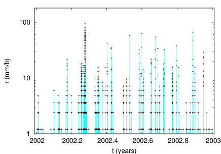
(a)

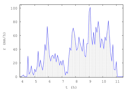
(b)

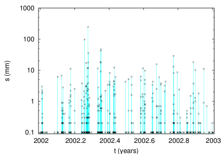
(c)

Abbildung 1: (a) Subset of the rain rate time series for site 17 (Muga) for year 2002. (b) More reduced subset of the rain rate time series for the same site, corresponding to the largest rain event on the record, with $s=248.7$ mm, on April 11, 2002. Time refers to hours since midnight. A very small rain event is also present at the beginning, with $s=0.3$ mm and separated to the main event by a dry spell of duration $q=15$ min. (c) Corresponding event-size time series for the same site, for year 2002.

1.2 Rain event sizes, rain event durations, and dry spell durations

Following Andrade et al. (1998) and Peters et al. (2002), we define a rain event as a sequence of consecutive rain rates bigger than zero delimited by zero rates, i.e., $\{r(t_{n}),r(t_{n+1}),\dots r(t_{m})\}$, such that $r(t_{i})>0$ for $i=n,n+1,\dots m$ with $r(t_{n-1})=r(t_{m+1})=0$. Due to the resolution of the record, this is equivalent to take a threshold with a value below 1.2 mm/hour. It is worth mentioning that this simple definition of rain events may be in conflict with those used by the hydrologists’ community, so caution is required in order to make comparisons between the different approaches (Molini et al., 2011).

The first observable to consider is

the duration $d$ of the event, which is the time that the event lasts (a multiple of 5 min, in our case). The size of the event is defined as the total rain during the event, i.e., the rate integrated over the event duration,

$$s\equiv\sum_{i=n}^{m}r(t_{i})\Delta t\simeq\int_{t_{n}}^{t_{m}}r(t)dt,$$

measured in mm (and multiple of 0.1 mm in our case, 1.2 mm/hr $\times$ 5 min). Notice that this event size is not the same as the usual rain depth, due to the different definition of the rain event in each case. Figure  1b shows as an illustration the evolution of the rate for the largest event in the record, which happens at the Muga site, whereas Fig. 1c displays the sequence of all event sizes in the same site for the year 2002. It is important to realize that this quantity is different to the one at Fig. 1a. Regarding event durations, the time series have a certain resemblance to Fig. 1c, as usually they are (nonlinearly) correlated with event sizes (Telesca et al., 2007). Further, the dry spells are the periods between consecutive rain events (then, they verify $r(t)=0$); we denote their durations by $q$. When a rain event, or a dry spell, is interrupted due to missing data, we discard that event or dry spell, and count the recorded duration as discarded time; the fraction of these times in the record appears in Table 1, under the symbol $f_{D}$. Although in some cases the duration of the interrupted event or dry spell can be bounded from below or from above (as in censored data), we have not attempted to use that partial information.

2 Power-law Distributions

2.1 Probability densities

Due to the enormous variability of the 3 quantities just defined, the most informative approach is to work with their probability distributions. Taking the size as an example, its probability density $P(s)$ is defined as the probability that the size is between $s$ and $s+ds$ divided by $ds$, with $ds\rightarrow 0$. Then, $\int_{0}^{\infty}P(s)ds=1$. This implicitly assumes that $s$ is considered as a continuous variable (but this will be corrected later, see more details on Appendix A). In general, we illustrate all quantities with the event size $s$, the analogous for $d$ and $q$ are obtained by replacing $s$ with the symbol of each observable. The corresponding probability densities are denoted as $P(d)$ and $P(q)$, with the implicit understanding that their functional forms may be different. Note that the annual number densities (Peters et al., 2002; Peters and Christensen, 2002, 2006) are trivially recovered multiplying the probability densities by the total number of events or dry spells and dividing by total time.

The results for the probability densities $P(s)$, $P(d)$, and $P(q)$ of all the sites under study are shown in Figs. 2a, 2b, and 2c, respectively. In all cases the distributions show a very clear behavior, monotonically decreasing and covering a broad range of values. However, to the naked eye, a power-law range is only apparent for the distributions of dry spells, $P(q)$ (remember that a power law turns into a straight line in a log-log plot). Moreover, the $P(q)$ are the broadest distributions, covering a range of more than 4 orders of magnitude (from 5 min to about a couple of months), and present in some cases a modest daily peak (in comparison to Peters et al. (2002), with 1 day $=$ 1440 min). In the opposite side we find the distributions of durations, $P(d)$, whose range is the shortest, from 5 min to about 1 day (two and a half orders of magnitude), and for which no straight line is visible in the plot; rather, the distributions appear as convex. The size distributions, $P(s)$, defined for about 3 orders of magnitude (from 0.1 to 200 mm roughly), can be considered in between the other two cases, with a visually shorter range of power-law behavior.

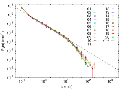
(a)

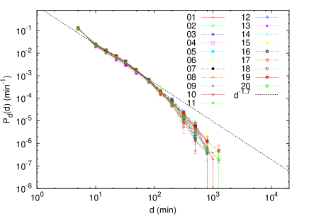
(b)

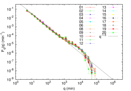
(c)

Abbildung 2: Probability densities for all the sites for the whole time covered by the record of: (a) Event sizes, (b) Event durations, and (c) Dry spells.

2.2 Fitting and testing power laws

A quantitative method can put more rigor into these observations. The idea is based on the recipe proposed by Clauset et al. (2009) – see also Corral et al. (2011) – but improved and generalized to our problem. Essentially, an objective procedure is required in order to find the optimum range in which a power law may hold. Taking again the event size for illustration, we report the power-law exponent fit between the values of $s_{\mathrm{min}}$ and $s_{\mathrm{max}}$ which yield the maximum number of data in that range but with a $p-$value greater than $10\%$. The method is described in detail in Peters et al. (2010), but we summarize it in the next paragraphs.

For a given value of the pair $s_{\mathrm{min}}$ and $s_{\mathrm{max}}$, the maximum-likelihood (ML) power-law exponent is estimated for the events whose size lies in that range. This exponent yields a fit of the distribution, and the goodness of such a fit is evaluated by means of the Kolmogorov-Smirnov (KS) test (Press et al., 1992). The purpose is to get a $p-$value, which is the probability that the KS test gives a distance between true power-law data and its fit larger than the distance obtained between the empirical data and its fit.

For instance, $p=20\%$ would mean that truly power-law distributed data were closer than the empirical data to their respective fits in $80\%$ of the cases, but in the rest $20\%$ of the cases a true power law were at a larger distance than the empirical data. So, in such a case the KS distance turns out to be somewhat large, but not large enough to reject that the data follow a power law with the ML exponent.

As in the case in which some parameter is estimated from the data there is no closed formula to calculate the $p-$value, we perform Monte Carlo simulations in order to compute the statistics of the Kolmogorov-Smirnov distance and from there the $p-$value. In this way, for each $s_{\mathrm{min}}$ and $s_{\mathrm{max}}$ we get a number of data $\bar{N}_{s}$ in that range and, repeating the procedure many times, a $p-$value. We look for the values of the extremes ($s_{\mathrm{min}}$ and $s_{\mathrm{max}}$) which maximize the number of data in between but with the restriction that the $p-$value has to be greater than $10\%$ (this threshold is arbitrary, but the conclusions do not change if it is moved). The maximization is performed sweeping 100 values of $s_{\mathrm{min}}$ and 100 values of $s_{\mathrm{max}}$, in log-scale, in such a way that all possible ranges (within this log-resolution) are taken into account. We have to remark that, in contrast with Peters et al. (2010), we have considered always discrete probability distributions, both in the ML fit and in the simulations. Of course, it is a matter of discussion which approach (continuous or discrete) is more appropriate for discrete data that represent a continuous process. In any case, the differences in the outcomes are rather small. Notice also that the method is not based on the estimation of the probability densities shown in the previous subsections, what would be inherently more arbitrary (Clauset et al., 2009).

The results of this method are in agreement with the visual conclusions obtained in the previous subsection, as can be seen in Table 2. Starting with the size statistics, 13 out of the 20 sites yield reasonable results, with an exponent $\tau_{s}$ between 1.43 and 1.54 over a logarithmic range $s_{\mathrm{max}}/s_{\mathrm{min}}$ from 12 to more than 200. For the rest of the sites, the range is too short, less than one decade (a decade is understood from now as an order of magnitude). In the application of the algorithm, it has been necessary to restrict the value of $s_{\mathrm{min}}$ to be $s_{\mathrm{min}}\geq 0.2$ mm; otherwise, as the distributions have a concave shape (in logscale) close to the origin (which means that there are many more events in that scale than at larger scales), the algorithm (which maximizes the number of data in a given range) prefers a short range with many data close to the origin than a larger range with less data away from the origin. It is possible that a variation of the algorithm in which the quantity that is maximized were different (for instance related with the range), would not need the restriction in the minimum size.

For the distribution of durations the resulting power laws turn out to be very limited in range; only 4 sites give not too short power laws, with $d_{max}/d_{min}$ from 6 to 12 and $\tau_{d}$ from 1.66 to 1.74. The other sites yield extremely short ranges for the power law be of any relevance. The situation is analogous to the case of the distribution of sizes, but the resulting ranges are much shorter here (Peters et al., 2010). Notice that the excess of events with $d=5$ min, eliminated from the fits imposing $d_{min}\geq 10$ min, has no counterpart in the value of the smallest rate (not shown), and therefore, we conclude that this extra number of events is due to problems in the time resolution of the data.

Considerably more satisfactory are the results for the dry spells. 16 sites give consistent results, with $\tau_{q}$ from 1.45 to 1.55 in a range $q_{max}/q_{min}$ from 30 to almost 300. It is noticeable that in these cases $q_{max}$ is always below 1 day. The removal by hand of dry spells around that value should enlarge a little the power-law range. In the rest of sites, either the range is comparatively too short (for example, for the Gaià site, the power-law behavior of $P(q)$ is interrupted at around $q=100$ min), or the algorithm has a tendency to include the bump the distributions show between the daily peak ($q$ beyond 1000 min) and the tail. This makes the value of the exponent smaller (around 1.25). Nevertheless, the value of the exponent is much higher than the one obtained for the equivalent problem of earthquake waiting times, where the Omori law leads to values around one, or  less. This points to a fundamental differencesbetween both kind of processes (from a statistical point of view).

In summary, the power laws for the distributions of durations are too short to be relevant, and the fits for the sizes are in the limit of what is acceptable (some cases are clear and some other not). Only the distributions of dry spells give really good power laws, with $\tau_{q}=1.50\pm 0.05$, and for more than two decades in 6 sites.

Tabelle 2: Results of the power-law fitting and goodness-of-fit tests applied to event sizes, event durations, and dry-spell durations (in mm or in min), for the period of 9 and a half years specified in the main text. The table displays the minimum of the fitting range, $s_{min}$, and the ratio between the maximum and the minimum of the fitting range (logarithmic range, $s_{max}/s_{min}$), total number of events, number of events in fitting range ($\bar{N}_{s}$, $\bar{N}_{d}$, and $\bar{N}_{q}$, for $s$, $d$, and $q$, respectively), and the power-law exponent with its uncertainty (one standard deviation) calculated as stated by Bauke (2007) and displayed between parenthesis as the variation of the last digit.

Site	$s_{min}$	$\frac{s_{max}}{s_{min}}$	$N_{s}$	$\bar{N_{s}}$	$\tau_{s}$
1	0.2	180.5	5393	1886	1.54(2)
2	0.2	4.5	5236	1323	1.64(6)
3	0.2	155.5	5749	2111	1.53(2)
4	0.2	12.0	5108	1745	1.43(3)
5	0.2	140.0	5289	2106	1.52(2)
6	0.2	68.0	4924	1969	1.49(2)
7	0.2	105.5	5219	2234	1.51(2)
8	0.2	213.0	5112	2047	1.53(2)
9	0.2	5.0	5366	1459	1.53(5)
10	0.2	19.0	6691	2452	1.51(2)
11	0.2	65.0	6224	2373	1.49(2)
12	0.2	4.0	5967	1500	1.53(6)
13	0.3	66.7	8330	1853	1.45(2)
14	0.2	3.5	6525	1711	1.56(6)
15	0.3	3.7	6485	1102	1.39(7)
16	0.2	3.5	7491	1852	1.59(5)
17	0.2	80.5	6962	2853	1.52(2)
18	0.2	41.5	7511	2847	1.51(2)
19	0.2	99.5	6767	2742	1.47(2)
20	0.2	3.5	9012	2047	1.69(5)

$d_{min}$	$\frac{d_{max}}{d_{min}}$	$\bar{N_{d}}$	$\tau_{d}$
10	10.0	1668	1.67(4)
10	4.0	1581	1.60(6)
10	6.0	1726	1.66(5)
10	3.5	1564	1.41(7)
10	3.5	1530	1.58(7)
10	3.5	1441	1.59(7)
10	3.5	1621	1.51(7)
10	4.0	1567	1.55(6)
10	4.0	1658	1.51(6)
10	3.5	2066	1.57(6)
10	5.0	1932	1.56(5)
10	4.0	1889	1.49(6)
10	12.5	2288	1.74(3)
10	5.0	2299	1.62(4)
10	5.0	2095	1.64(5)
10	4.0	2385	1.59(5)
10	3.5	2087	1.60(6)
10	3.5	2238	1.57(6)
10	3.5	1958	1.60(6)
10	8.5	2972	1.66(3)

$q_{min}$	$\frac{q_{max}}{q_{min}}$	$N_{q}$	$\bar{N_{q}}$	$\tau_{q}$
95	7.8	5387	743	1.75(7)
5	273.0	5231	4729	1.46(1)
10	80.0	5745	3207	1.53(2)
5	196.0	5103	4520	1.47(1)
20	47.3	5287	1706	1.45(2)
20	31.3	4926	1537	1.47(3)
5	256.0	5215	4734	1.51(1)
15	65.0	5107	2098	1.50(2)
10	90.0	5419	2889	1.55(2)
25	33.0	6685	1758	1.48(3)
45	468.3	6219	2005	1.24(1)
5	235.0	5961	5376	1.47(1)
130	158.5	8328	1501	1.27(2)
5	215.0	6520	5906	1.47(1)
15	49.7	6479	2560	1.51(2)
5	214.0	7510	6789	1.50(1)
10	68.5	6958	3719	1.52(1)
20	31.0	7507	2302	1.53(2)
50	21.7	6800	1378	1.26(3)
15	34.3	9007	3367	1.50(2)

3 Scaling

3.1 Non-parametric scaling

However, the fact that a power-law behavior does not exist over a broad range of values does not rule out the existence of SOC (Christensen and Moloney, 2005). In fact, the fulfillment of a power-law distribution in the form of Eq. (1) is only valid when finite-size effects are “small”, which only happens for large enough systems. In general, when these effects are taken into account, SOC behavior leads to distributions of the form (Christensen and Moloney, 2005; Peters et al., 2010),

$$P(s)=s^{-\tau_{s}}\mathcal{G}_{s}(s/s_{\xi})\mbox{ \, for \,}s>s_{l},$$ (2)

where $\mathcal{G}_{s}(x)$ is a scaling function that is essentially constant for $x\ll 1$ and decays fast for $x\gg 1$, accounting in this way for the finite-size effects when $s$ is above the crossover value $s_{\xi}$; the size $s_{l}$ is just a lower cutoff limiting the validity of this description. The pure power law only emerges for $s_{\xi}\rightarrow\infty$, nevertheless, a truncated power law holds over an appreciable range if the scales given by $s_{l}$ and $s_{\xi}$ are well separated, i.e., $s_{l}\ll s_{\xi}$. As $s_{\xi}$ increases with system size, typically as $s_{\xi}\propto L^{D_{s}}$ (with $D_{s}$ the so-called avalanche dimension, or event-size dimension), the power-law condition (1) can only be fulfilled for large enough system sizes.

Note that, in the case of a too short power-law range or a non-conclusive fit, we still could check the existence of scaling using Eq. (2) if we knew $s_{\xi}$ or $L$. However, $s_{\xi}$ is difficult to measure, needing a parameterization of the scaling function, and it is not clear what the system size $L$ is for rainfall. It could be the vertical extension of the clouds, or the depth of the troposphere. Nevertheless, it is important to realize that the scaling ansatz (2) still can be checked from data without knowledge of $L$ or $s_{\xi}$. First, notice that the ansatz implies that the $k-$order moment of $s$ scales with $L$ as

$$\langle s^{k}\rangle\propto L^{D_{s}(k+1-\tau_{s})}\mbox{ \, for \,}1<\tau_{s}<k+1,$$ (3)

if $s_{l}\ll s_{\xi}$, see Christensen and Moloney (2005). Second, Eq. (2) can be written in a slightly different form, as a scaling law,

$$P(s)=L^{-D_{s}\tau_{s}}\mathcal{F}_{s}(s/L^{D_{s}})\mbox{ \, for \,}s>s_{l},$$ (4)

where the new scaling function $\mathcal{F}_{s}(x)$ is defined as $\mathcal{F}_{s}(x)\equiv x^{-\tau_{s}}\mathcal{G}_{s}(x/a)$ ($a$ is the constant of proportionality between $s_{\xi}$ and $L^{D_{s}}$). This form of $P(s)$ (in fact, $P(s,L)$), with an arbitrary $\mathcal{F}$, is the well-known scale-invariance condition for functions with two variables (Christensen and Moloney, 2005). Changes of scale (linear transformations) in $s$ and $L$ may leave the shape of the function $P(s,L)$ unchanged (this is what scale invariance really means, power laws are just a particular case in one dimension).

Substituting $L^{D_{s}}\propto\left\langle s^{2}\right\rangle/\left\langle s\right\rangle$ and $L^{D_{s}\tau_{s}}\propto L^{2D_{s}}/\left\langle s\right\rangle\propto\left\langle s^{2}\right\rangle^{2}/\left\langle s\right\rangle^{3}$ (from the scaling of $\left\langle s^{k}\right\rangle$, assuming $\tau_{s}<2$) into Eq. (4) leads to

$$P(s)=\left\langle s\right\rangle^{3}\left\langle s^{2}\right\rangle^{-2}\tilde{\mathcal{F}}_{s}(s\left\langle s\right\rangle/\left\langle s^{2}\right\rangle),$$ (5)

where $\tilde{\mathcal{F}}_{s}(x)$ is essentially the scaling function ${\mathcal{F}}_{s}(x)$, absorbing the proportionality constants. Therefore, if scaling holds, a plot of $\left\langle s^{2}\right\rangle^{2}P(s)/\left\langle s\right\rangle^{3}$ versus $s\left\langle s\right\rangle/\left\langle s^{2}\right\rangle$ for all the sites has to yield a collapse of the distributions into a single curve, which draws $\tilde{\mathcal{F}}_{s}(x)$ (a similar procedure is outlined in Rosso et al. (2009)). In order to proceed, the mean and the quadratic mean, $\left\langle s\right\rangle$ and $\left\langle s^{2}\right\rangle$, can be easily estimated from data. Since no estimation of parameters is involved for this procedure, we call it non-parametric scaling.

The outcome for $P(s)$, $P(d)$, and $P(q)$ is shown in Figs. 3a, 3b, and 3c, with reasonable results, especially for the distribution of dry spells. The plot suggests that the scaling function $\mathcal{G}_{q}$ of the dry-spell distribution has a maximum around $x\simeq 1$, but this does not in disagreement with our approach, which only assumed a constant scaling function for small $x$ and a fast decay for large $x$.

Note that the quotient $\left\langle s^{2}\right\rangle/\left\langle s\right\rangle$ gives the scale for the crossover value $s_{\xi}$ (as $s_{\xi}\propto\left\langle s^{2}\right\rangle/\left\langle s\right\rangle$, with a constant of proportionality that depends on the scaling function $\mathcal{G}_{s}$ and on $s_{l}/s_{\xi}$), and therefore it is the ratio of the second moment to the mean and not the mean which describes the scaling behavior of the distribution. This can have important implications for extreme events: an increase in the value of the mean is not proportional to an increase of the most extreme events, represented by $s_{\xi}$. For the case of event sizes, we get values of $\left\langle s^{2}\right\rangle/\left\langle s\right\rangle$ between 10 and 30 mm (which is a variability much higher than that of $\left\langle s\right\rangle$), and therefore the condition $s_{l}\ll s_{\xi}$ is very well fulfilled (assuming that the moment ratio $\left\langle s^{2}\right\rangle/\left\langle s\right\rangle$ is of the same order as $s_{\xi}$, and with $s_{l}\simeq s_{min}$), which is a test for the consistency of our approach. For dry spells $\left\langle q^{2}\right\rangle/\left\langle q\right\rangle$ is between 5 and 13 days, which is even better for the applicability of the scaling analysis. The case of the event durations is somewhat “critical”, with $\left\langle d^{2}\right\rangle/\left\langle d\right\rangle$ between 70 and 120 min, which yields $d_{\xi}/d_{l}$ in the range from 14 to 24. Nevertheless, we observe that the condition $s_{l}\ll s_{\xi}$ for the power law to show up is stronger than the same condition for the scaling analysis to be valid.

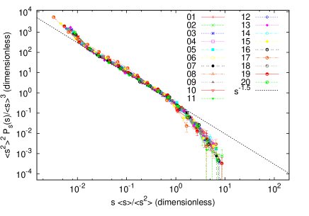
(a)

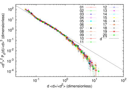
(b)

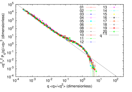
(c)

Abbildung 3: Collapse of the probability densities for all the sites for the whole time covered by the record of: (a) Event sizes, (b) Event durations, and (c) Dry spells. Rescaling is performed using the first and second moment of each distribution, following Eq. (5).

3.2 Parametric scaling

Further, a scaling ansatz as Eq. (2) or (4) allows an estimation of the exponent $\tau_{s}$, even in the case in which a power law cannot be fit to the data. From the scaling of the moments of $s$ we get, taking $k=1$, $L^{D_{s}}\propto\left\langle s\right\rangle^{1/(2-\tau_{s})}$ and $L^{D_{s}\tau_{s}}\propto\left\langle s\right\rangle^{\tau_{s}/(2-\tau_{s})}$ (again with $\tau_{s}<2$); so, substituting into Eq. (4),

$$P(s)=\left\langle s\right\rangle^{-\tau_{s}/(2-\tau_{s})}\hat{\mathcal{F}}_{s}(s/\left\langle s\right\rangle^{1/(2-\tau_{s})}).$$ (6)

One only needs to find the value of $\tau_{s}$ that optimizes the collapse of all the distributions, i.e., that makes the previous equation valid, or at least as close to validity as possible. As the scaling depends on the parameter $\tau_{s}$, we refer to this procedure as parametric scaling.

We therefore need a measurement to quantify distance between rescaled distributions. In order to do that, we have chosen to work with the cumulative distribution function, $S(s)\equiv\int_{s}^{\infty}P(s^{\prime})ds^{\prime}$, rather than with the density (to be rigorous, $S(s)$ is the complementary of the cumulative distribution function, and is called survivor function or reliability function in some contexts). Although in practice both $P(s)$ and $S(s)$ contain the same probabilistic information, the reason to work with $S(s)$ is double: the estimation of the cumulative distribution function does not depend of an arbitrarily selected bin width $ds$ (Press et al., 1992), and it does not give equal weight to all scales in the representation of the function (i.e., in the number of points that constitute the function). The scaling laws (4) and (6) turn out to be, then,

$$S(s)=L^{-D_{s}(\tau_{s}-1)}\mathcal{H}_{s}(s/L^{D_{s}}),$$ (7)

$$S(s)=\left\langle s\right\rangle^{-(\tau_{s}-1)/(2-\tau_{s})}\hat{\mathcal{H}}_{s}(s/\left\langle s\right\rangle^{1/(2-\tau_{s})}),$$ (8)

with ${\mathcal{H}_{s}}(x)$ and $\hat{\mathcal{H}_{s}}(x)$ the corresponding scaling functions.

The first step of the method of collapse is to merge all the pairs $\{s,S(s)\}_{i}$ into a unique rescaled function $\{x,y\}$. If $i=1,\dots,20$ runs for all sites, and $j=1,\dots,M_{s}(i)$ for all the different values that the size of events takes on site $i$ (note that $M_{s}(i)\leq N_{s}(i)$), then,

$$x_{\ell}(\tau)\equiv\log(s_{ji}/\left\langle s\right\rangle_{i}^{1/(2-\tau)}),$$

$$y_{\ell}(\tau)\equiv\log(S_{i}(s_{ji})\left\langle s\right\rangle_{i}^{(\tau-1)/(2-\tau)}),$$

with $s_{ji}$ the $j$-th value of the size in site $i$, $\left\langle s\right\rangle_{i}$ the mean on $s$ in $i$, $S_{i}(s_{ji})$ the cumulative distribution function in $i$, and $\tau$ a possible value of the exponent $\tau_{s}$. The index $\ell$ labels the new function, from 1 to $\sum_{\forall i}M_{s}(i)$, in such a way that $x_{\ell}(\tau)\leq x_{\ell+1}(\tau)$; i.e., the pairs $x_{\ell}(\tau),y_{\ell}(\tau)$ are sorted by increasing $x$.

Then, we just compute

$$D(\tau)\equiv\sum_{\forall\ell}\left([x_{\ell}(\tau)-x_{\ell+1}(\tau)]^{2}+[y_{\ell}(\tau)-y_{\ell+1}(\tau)]^{2}\right),$$ (9)

which represents the sum of all Euclidean distances between the neighboring points in a (tentative) collapse plot in logarithmic scale. The value of $\tau$ which minimizes this function is identified with the exponent $\tau_{s}$ in Eq. (2). We have tested the algorithm applying it to SOC models whose exponents are well known (not shown).

The results of this method applied to our datasets, not only for the size distributions but also to the distributions of $d$, are highly satisfactory. There is only one requirement: the removal of the first point in each distribution ($s=0.1$ mm and $d=5$ min), as with the ML fits. The exponents we find are $\tau_{s}=1.52\pm 0.12$ and $\tau_{d}=1.69\pm 0.01$, in agreement with the ones obtained by the power-law fitting method presented above; the corresponding rescaled plots are shown in Fig. 4. Although the visual display does not allow to evaluate properly the quality of the collapse, the reduction in the value of the function $D(\tau)$ is notable. Then, the performance of the method is noteworthy, taking into account that the mean values of the distributions show little variation in most cases. In addition, the shape of the scaling function $\mathcal{G}_{s}$ can be obtained by plotting, as suggested by Eq. (2), $s^{\tau_{s}}P(s)$ versus $s/\left\langle s\right\rangle^{1/(2-\tau_{s})}$, and the same for the other variable, $d$. Figure  5 displays what is obtained for each distribution. In contrast, the application of this method to $P(q)$ does not yield consistent results, as $\tau_{q}$ turns out to be rather small (1.24). Notice that the existence of a daily peak in the distributions is an obstacle to a data collapse, as the peak prevents a good scaling.

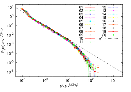
(a)

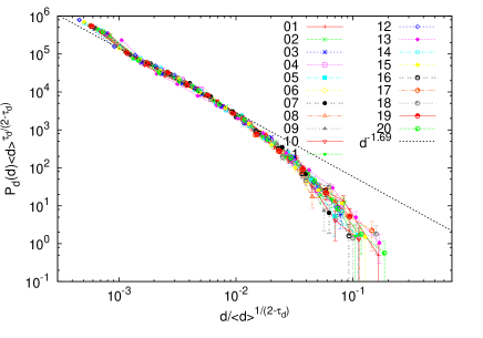
(b)

Abbildung 4: Collapse of the probability densities for all the sites for the whole time covered by the record of: (a) Event sizes and (b) Event durations; rescaled using Eq. (6) with the exponents: $\tau_{s}=1.52$ and $\tau_{d}=1.69$, determined minimizing the Euclidean distance between parametrically collapsed distributions. Units are mm or min to the corresponding powers appearing in the axes.

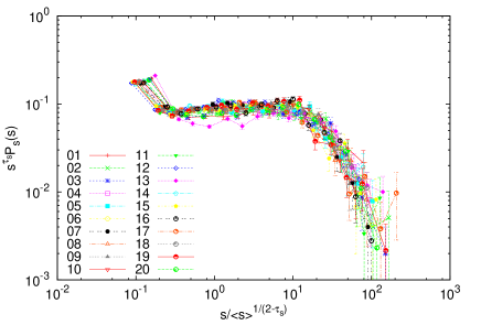
(a)

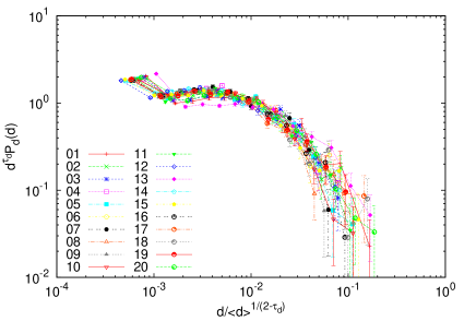
(b)

Abbildung 5: Inferred scaling functions $\mathcal{G}_{s}$ and $\mathcal{G}_{d}$ corresponding to the rescaled distributions of $s$ and $d$ in Fig. 4, multiplied by $s^{\tau_{s}}$ and $d^{\tau_{d}}$. Units in the abscissae are as in the previous plot, whereas in the ordinates these are mm${}^{\tau_{s}-1}$ and min${}^{\tau_{d}-1}$.

[Discussion and Conclusions]

We have performed an in-depth study of the properties of SOC related observables in rainfall in the Mediterranean region in order to check if this framework can be useful for modeling rain events and dry spells. The results support this hypothesis, which had not been checked before in this region or for this kind of data resolution. For the distributions of rain-event sizes we get power-law exponents valid for one or two decades in the majority of sites, with exponent values $\tau_{s}\simeq 1.50\pm 0.05$. For the distributions of event durations, the fitting ranges are shorter, reaching in the best case one decade, with exponents $\tau_{d}\simeq 1.70\pm 0.05$. This range is expected to be shorter than for event sizes, given that these combine the event duration distribution with the rain rate (Peters et al., 2010). And finally, the dry spell distributions yield the more notable power law fits, with exponents in the range $\tau_{q}\simeq 1.50\pm 0.05$, in some cases for more than 2 decades.

These results are compatible with the ones obtained for the Baltic sea by Peters et al. (2002), which yielded $\tau_{s}\simeq\tau_{q}\simeq 1.4$ and $\tau_{d}\simeq 1.6$. The agreement is remarkable, taking into account the different nature of the data analyzed and the disparate fitting procedures. However, the concordance with the more recent results of Peters et al. (2010) is not very good, quantitatively. That previous study, with a minimum detection rate of 0.2 mm/hr and a time resolution $\Delta t=1$ min, found $\tau_{s}\simeq 1.18$ for several sites across different climates, using essentially the same statistical techniques as in the present study. Exponents were found not universal for durations of events and dry-spells, but for the latter they were close in many cases to $\tau_{d}\simeq 1.3$. The difference between the size and dry-spell duration exponents may be due to data resolution. Changes in the detection threshold have a non-trivial repercussion in the size and duration of the events and the dry spells (an increase in the threshold can split one single event into two or more separate ones but also can remove events). Further, better time resolution and lower detection threshold allow the detection of smaller events, enlarging the power law range and reducing the weight from the part close to the crossover point (where the distribution becomes steeper); this trivially leads to smaller values of the exponent. In the dry spells case, the power-law range in this study is enough to guarantee that our estimation of the exponents are robust, so the discrepancy with Peters et al. (2010) may be due to the non-trivial effect of the change in the detection thresholds or differences on the measurement devices.

On the other hand, finite size effects can explain the limited power-law range obtained for $s$ and $d$ observables, as it occurs in other (self-organized and non-self-organized) critical phenomena. The finite-size analysis performed, in terms of combinations of powers of the moments of the distributions, supports this conclusion. The collapse of the distributions is a clear signature of scale-invariance: different sites share a common shape of the rain-event and dry-spell distributions, with differences in the scale of those distributions, depending on system size. Then, in the ideal case of an infinite system, the power laws would lack an upper cutoff. Moreover, the collapse of the distributions allows an independent estimate of the power-law exponents, which, for event durations and sizes, are in surprising agreement with the values obtained by the maximum-likelihood fit. For dry spell durations, a daily peak in the distributions hinders their collapse.

Nevertheless, future work should consider spatially extended events. Our measurements are taken in a point of the system which reflects information on the vertical scale, then, the results could be affected by this. Another important issue are the implications of the results for hazard assessment. If there is not a characteristic rain-event size, then there is neither a definite separation nor a fundamental difference between the smallest harmless rains and the most hazardous storms. Further, it is generally believed that the critical evolution of events in SOC systems implies that, at a given instant, it is equally likely that the event intensifies or weakens, which would make detailed prediction unattainable. However, this view has been recently proved wrong, as it has been reported that a critical evolution describes the dynamics of some SOC systems only on average; further, the existence of finite size effects can be used for prediction (Garber et al., 2009; Martin et al., 2010). Interestingly, in the case of rain, it has been recently shown by Molini et al. (2011) that knowledge of internal variables of the system allows some degree of prediction for the duration of the events, related also to the departure of the system from quasi-equilibrium conditions. Finally, we urge studies which explore the effects of resolution and detection-threshold value in high-resolution rain data. A common SOC misbelief is that avalanches happen following a memoryless process, leading therefore to exponential distributions for the waiting times (Corral, 2005). This has been proved wrong if a threshold on the intensity is present (Paczuski et al., 2005). In this case, times between avalanches follow a power-law distribution, as we find for dry spells.

In summary, we conclude that the statistics of rainfall events in the NW Mediterranean area studied are in agreement with the SOC paradigm expectations. This is the first time this study is realized for this region and it is a confirmation of what has been found for other places of the world, but using in ourcase data with lower resolution. If a representative universal exponent existed, this would mean that just one parameter is enough for characterizing the distributions. This would indicate that the rain event observable cannot detect climatic differences between regions, but would shed light on universal properties and mechanisms of rainfall generation.

Anhang A

Details on the estimation of the probability density

In practice, the estimation of the density from data is performed taking a value of $ds$ large enough to guarantee statistical significance, and then compute $P(s)$ as $n(s)/(N_{s}\Delta)$, where $n(s)$ is the number of events with size in the range between $s$ and $s+ds$, $N_{s}$ the total number of events, and $\Delta$ is defined as

$$\Delta=R_{s}(\lfloor(s+ds)/R_{s}\rfloor-\lfloor s/R_{s}\rfloor),$$

with $\lfloor x\rfloor$ the integer part of $x$ and $R_{s}$ the resolution of $s$, i.e. $R_{s}=0.1$ mm (but note that high resolution means low $R_{s}$). So, $\Delta/R_{s}$ is the number of possible different values of the variable in the interval considered. Notice that using $\Delta$ instead of $ds$ in the denominator of the estimation of $P(s)$ allows one to take into account the discreteness of $s$. If $R_{s}$ tended to zero, then $\Delta\rightarrow ds$ and the discreteness effects would become irrelevant.

How large does $ds$ have to be to guarantee the statistical significance of the estimation of $P(s)$? Working with long-tailed distributions (where the variable covers a broad range of scales) a very useful procedure is to take a width of the interval $ds$ that is not the same for all $s$, but that is proportional to the scale, as $[s,s+ds)=[s_{o},bs_{o})$, $[bs_{o},b^{2}s_{o})$, $\dots$ $[b^{k}s_{o},b^{k+1}s_{o})$, i.e., $ds=(b-1)s$ (with $b>1$). Given a value of $s$, the corresponding value of $k$ that associates $s$ with its bin is given by $k=\lfloor\log_{b}(s/s_{o})\rfloor$. Correspondingly, the optimum choice to assign a point to the interval $[s,s+ds)$ is given by the value $\sqrt{b}s$. This procedure is referred to as logarithmic binning, because the intervals appear with fixed width in logarithmic scale (Hergarten, 2002). In this paper we have generally taken $b\simeq 1.58$, in such a way that $b^{5}=10$, providing 5 bins per order of magnitude.

As the distributions are estimated from a finite number of data, they display statistical fluctuations. The uncertainty characterizing these fluctuations is simply related to the density by

$$\frac{\sigma_{P}(s)}{P(s)}\simeq\frac{1}{\sqrt{n(s)}},$$

where $\sigma_{P}(s)$ is the standard deviation of $P(s)$ (do not confound with the standard deviation of $s$). This is so because $n(s)$ can be considered a binomial variable (von Mises, 1964), and then, the ratio between its standard deviation and mean fulfills $\sigma_{n}(s)/\langle n(s)\rangle\simeq 1/\sqrt{n(s)}$, with $n(s)/N_{s}\ll 1$. As $P(s)$ is proportional to $n(s)$, the same relation holds for its relative uncertainty.