Janus fluid with fixed patch orientations: theory and simulations

Abstract

We study thermophysical properties of a Janus fluid with constrained orientations, using analytical techniques and numerical simulations. The Janus character is modeled by means of a Kern–Frenkel potential where each sphere has one hemisphere of square-well and the other of hard-sphere character. The orientational constraint is enforced by assuming that each hemisphere can only point either North or South with equal probability. The analytical approach hinges on a mapping of the above Janus fluid onto a binary mixture interacting via a “quasi” isotropic potential. The anisotropic nature of the original Kern–Frenkel potential is reflected by the asymmetry in the interactions occurring between the unlike components of the mixture. A rational-function approximation extending the corresponding symmetric case is obtained in the sticky limit, where the square-well becomes infinitely narrow and deep, and allows a fully analytical approach. Notwithstanding the rather drastic approximations in the analytical theory, this is shown to provide a rather precise estimate of the structural and thermodynamical properties of the original Janus fluid.

I Introduction

Janus fluids refer to colloidal suspensions formed by nearly spherical particles with two different philicities evenly distributed in the two hemispheres.Pawar10 ; Walther08 Under typical experimental conditions in a water environment, one of the two hemispheres is hydrophobic, while the other is charged, so that different particles tend to repel each other, hence forming isolated monomers. On the other hand, if repulsive forces are screened by the addition of a suitable salt, then clusters tend to form driven by hydrophobic interactions.Hong08

This self-assembly mechanism has recently attracted increasing attention due to the unprecedented improvement in the chemical synthesis and functionalization of such colloidal particles, that allows a precise and reliable control on the aggregation process that was not possible until a few years ago.Bianchi11 From a technological point of view, this is very attractive as it paves the way to a bottom-up design and engineering of nanomaterials alternative to conventional top-down techniques.Zhang04

One popular choice of model describing the typical duality characteristic of the Janus fluid is the Kern–Frenkel model.Kern03 This model considers a fluid of rigid spheres having their surfaces partitioned into two hemispheres. One of them has a square-well (SW) character, i.e., it attracts other similar hemispheres through a SW interaction, thus mimicking the short-range hydrophobic interactions occurring in real Janus fluids. The other part of the surface is assumed to have hard-sphere (HS) interactions with all other hemispheres, i.e., with both like HS as well as SW hemispheres. The HS hemisphere hence models the charged part in the limit of highly screened interactions that is required to have aggregation of the clusters.

Although in the present paper only an even distribution between SW and HS surface distributions will be considered (Janus limit), other choices of the coverage, that is the fraction of SW surface with respect to the total one, have been studied within the Kern–Frenkel model.Sciortino10 In fact, one of the most attractive features of the general model stems from the fact that it smoothly interpolates between an isotropic HS fluid (zero coverage) and an equally isotropic SW fluid (full coverage). Giacometti09 ; Giacometti10

The thermophysical and structural properties of the Janus fluid have been recently investigated within the framework of the Kern–Frenkel model using numerical simulations,Sciortino09 ; Sciortino10 thus rationalizing the cluster formation mechanism characteristic of the experiments.Hong08 The fluid-fluid transition was found to display an unconventional and particularly interesting phase diagram, with a re-entrant transition associated with the formation of a cluster phase at low temperatures and densities.Sciortino09 ; Sciortino10 While numerical evidence of this transition is quite convincing, a minimal theory including all necessary ingredients for the onset of this anomalous behavior is still missing. Two previous attempts are however noteworthy. Reinhardt et al.Reinhardt11 introduced a van der Waals theory for a suitable mixture of clusters and monomers that accounts for a re-entrant phase diagram, whereas Fantoni et al.Fantoni11 ; Fantoni12 developed a cluster theory explaining the appearance of some “magic numbers” in the cluster formation. This notwithstanding, the challenge of an analytical theory fully describing the anomaly occurring in the phase diagram of the Janus fluid still remains.

The aim of the present paper is to attempt a new route in this direction. We will do this by considering a Janus fluid within the Kern–Frenkel model, where the orientations of the SW hemispheres are constrained to be along either North or South, in a spirit akin to Zwanzig model for the isotropic-nematic transition in liquid crystals.Zwanzig63

Upon observing that under those conditions, one ends up with only four possible different interactions (North-North, North-South, South-North, and South-South), this constrained model will be further mapped onto a binary mixture interacting via a “quasi” isotropic potential. Here the term “quasi” refers to the fact that a certain memory of the original anisotropic Kern–Frenkel potential is left: after the mapping, one has to discriminate whether a particle with patch pointing North (“spin-up”) is lying above or below that with a patch pointing South (“spin-down”). This will introduce an asymmetry in the unlike components of the binary mixture, as explained in detail below. In order to make the problem tractable from the analytical point of view, the particular limit of an infinitely narrow and deep square-well (sticky limit) will be considered. This limit was originally devised by Baxter and constitutes the celebrated one-component sticky-hard-sphere (SHS) or adhesive Baxter model.Baxter68 By construction, our model reduces to it in the limit of fully isotropic attractive interactions. The latter model was studied within the Percus–Yevick (PY) closureHansen86 in the original Baxter work and in a subsequent work by Watts et al.Watts71 The extension of this model to a binary mixture was studied by several authors.PS75 ; Barboy75 ; Barboy79 ; Zaccarelli00 ; TKR02 The SHS model with Kern–Frenkel potential was also studied in Ref. Fantoni07, , via a virial expansion at low densities.

A methodology alternative to the one used in the above studies hinges on the so-called “rational-function approximation” (RFA),Santos98 ; deHaro08 and is known to be equivalent to the PY approximation for the one-component SHS Baxter modelBaxter68 and for its extension to symmetric SHS mixtures.PS75 ; Santos98 ; TKR02 The advantage of this approach is that it can be readily extended to more general cases, and this is the reason why it will be employed in the present analysis to consider the case of asymmetric interactions. We will show that this approach provides a rather precise estimate of the thermodynamic and structural properties of the Janus fluids with up-down orientations by explicitly testing it against Monte Carlo (MC) simulations of the same Janus fluid.

The remaining part of the paper is envisaged as follows. Section II describes our Janus model and its mapping onto a binary mixture with asymmetric interactions. It is shown in Sec. III that the thermophysical quantities do not require the knowledge of the full (anisotropic) pair correlation functions but only of the functions averaged over all possible North or South orientations. Section IV is devoted to the sticky-limit version of the model, i.e., the limit in which the SW hemisphere has a vanishing well width but an infinite depth leading to a constant value of the Baxter parameter $\tau$. The exact cavity functions to first order in density (and hence exact up to second and third virial coefficients) in the sticky limit are worked out in Appendix A. Up to that point all the equations are formally exact in the context of the model. Then, in Sec. V we present our approximate RFA theory, which hinges on a heuristic extension from the PY solution for mixtures with symmetric SHS interactions to the realm of asymmetric SHS interactions. Some technical aspects are relegated to Appendices B and C. The prediction of the resulting analytical theory are compared with MC simulations in Sec. VI, where a semi-quantitative agreement is found. Finally, the paper is closed with conclusions and an outlook in Sec. VII.

II Mapping the Kern–Frenkel potential onto a binary mixture

II.1 The Kern–Frenkel potential for a Janus fluid

Consider a fluid of spheres with identical diameters $\sigma$ where the surface of each sphere is divided into two parts. The first hemisphere (the green one in the color code given in Fig. 1) has a SW character, thus attracting another identical hemisphere via a SW potential of width $(\lambda-1)\sigma$ and depth $\epsilon$. The second hemisphere (the red one in the color code of Fig. 1) is instead a HS potential. The orientational dependent pair potential between two arbitrary particles $\mu$ and $\nu$ ($\mu,\nu=1,\ldots,N$, where $N$ is the total number of particles in the fluid) has then the form proposed by Kern and FrenkelKern03

$$\Phi\left(\mathbf{r}_{\mu\nu},\widehat{\mathbf{n}}_{\mu},\widehat{\mathbf{n}}_{\nu}\right) = \phi_{\text{HS}}\left(r_{\mu\nu}\right)+\phi_{\text{SW}}\left(r_{\mu\nu}\right)\Psi\left(\widehat{\mathbf{r}}_{\mu\nu},\widehat{\mathbf{n}}_{\mu},\widehat{\mathbf{n}}_{\nu}\right),$$

where the first term is the HS contribution

$$\phi_{\text{HS}}\left(r\right)=\begin{cases}\infty,&0<r<\sigma,\\ 0,&\sigma<r,\end{cases}$$ (2)

and the second term is the orientation-dependent attractive part, which can be factorized into an isotropic SW tail

$$\phi_{\text{SW}}\left(r\right)=\begin{cases}-\epsilon,&\sigma<r<\lambda\sigma,\\ 0,&\lambda\sigma<r,\end{cases}$$ (3)

multiplied by an angular dependent factor

$$\Psi\left(\widehat{\mathbf{r}}_{\mu\nu},\widehat{\mathbf{n}}_{\mu},\widehat{\mathbf{n}}_{\nu}\right)=\begin{cases}1,&\text{if }\widehat{\mathbf{n}}_{\mu}\cdot\widehat{\mathbf{r}}_{\mu\nu}\geq 0\text{ and }\widehat{\mathbf{n}}_{\nu}\cdot\widehat{\mathbf{r}}_{\mu\nu}\leq 0\\ 0,&\text{otherwise}.\end{cases}$$ (4)

Here, $\widehat{\mathbf{r}}_{\mu\nu}=\mathbf{r}_{\mu\nu}/r_{\mu\nu}$, where $\mathbf{r}_{\mu\nu}=\mathbf{r}_{\nu}-\mathbf{r}_{\mu}$, is the unit vector pointing (by convention) from particle $\mu$ to particle $\nu$ and the unit vectors $\widehat{\mathbf{n}}_{\mu}$ and $\widehat{\mathbf{n}}_{\nu}$ are “spin” vectors associated with the orientation of the attractive hemispheres of particles $\mu$ and $\nu$, respectively (see Fig. 1). An attractive interaction then exists only between the two SW portions of the surface sphere, provided that the two particles are within the range of the SW potential.

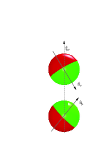
Figure 1: The Kern–Frenkel potential for Janus fluids.

II.2 Asymmetric binary mixture

We now consider the particular case where the only possible orientations of particles are with attractive caps pointing only either North or South with equal probability, as obtained by Fig. 1 in the limit $\widehat{\mathbf{n}}_{\mu}=\widehat{\mathbf{z}}$, $\widehat{\mathbf{n}}_{\nu}=-\widehat{\mathbf{z}}$, and with $\widehat{\mathbf{z}}$ pointing North.

Under these conditions, one then notes that the Kern–Frenkel potential (LABEL:mapping:eq1)–(4) can be simplified by associating a spin $i=1$ (up) to particles with SW hemispheres pointing in the North $\widehat{\mathbf{z}}$ direction and a spin $j=2$ (down) to particles with SW hemispheres pointing in the South $-\widehat{\mathbf{z}}$ direction, so one is left with only four possible configurations depending on whether particles of type $1$ lie above or below particles of type $2$, as illustrated in Fig. 2. The relationship between the genuine Janus model (see Fig. 1) and the up-down model (see Fig. 2) is reminiscent to the relationship between the Heisenberg and the Ising model of ferromagnetism. From that point of view, our model can be seen as an Ising-like version of the original Janus model. A similar spirit was also adopted in the Zwanzig model for the isotropic-nematic transition in liquid crystals.Zwanzig63

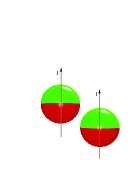
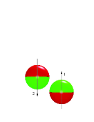
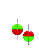
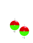
Figure 2: (Top-left) A particle of type $1$ is “below” another particle of type $1$ providing SW/HS=HS interactions. (Top-right) A particle of type $1$ is “below” a particle of type $2$ leading to SW/SW=SW interactions. (Bottom-left) A particle of type $2$ is “below” a particle of type $1$ yielding HS/HS=HS interactions. (Bottom-right) A particle of type $2$ is “below” another particle of type $2$ thus leading again to HS/SW=HS interactions.

The advantage of this mapping is that one can disregard the original anisotropic Janus-like nature of the interactions and recast the problem in the form of a binary mixture such that the interaction potential between a particle of species $i$ located at $\mathbf{r}_{1}$ and a particle of species $j$ located at $\mathbf{r}_{2}$ has the asymmetric form

$$\phi_{ij}(\mathbf{r}_{1},\mathbf{r}_{2}) = \phi_{ij}(\mathbf{r}_{12})$$

$$= \varphi_{ij}(r_{12})\Theta(\cos\theta_{12})+\varphi_{ji}(r_{12})\Theta(-\cos\theta_{12}),$$

where $\cos\theta_{12}=\widehat{\mathbf{r}}_{12}\cdot\widehat{\mathbf{z}}$ (recall our convention $\mathbf{r}_{12}=\mathbf{r}_{2}-\mathbf{r}_{1}$) and

$$\varphi_{ij}(r)=\phi_{\text{HS}}(r)+\begin{cases}\phi_{\text{SW}}(r),&\text{if }i=1\text{ and }j=2,\\ 0,&\text{otherwise}.\end{cases}$$ (6)

In Eq. (LABEL:mapping:eq5) $\Theta(x)=1$ and $0$ for $x>0$ and $x<0$, respectively.

It is important to remark that, in general, $\varphi_{12}(r)\neq\varphi_{21}(r)$, as evident from Eq. (6). Thus, the binary mixture is not necessarily symmetric [unless $\epsilon=0$ or $\lambda=1$ in Eq. (3)], unlike standard binary mixtures where this symmetry condition is ensured by construction. In the potential (LABEL:mapping:eq5), there however is still a “memory” of the original anisotropy since the potential energy of a pair of particles of species $i$ and $j$ separated a distance $r_{12}$ depends on whether particle $j$ is “above” ($\cos\theta_{12}>0$) or “below” ($\cos\theta_{12}<0$) particle $i$. In this sense, the binary mixture obtained in this way is “quasi”, and not “fully”, spherically symmetric.

Another important point to be stressed is that, while the sign of $\cos\theta_{12}$ represents the only source of anisotropy in the above potential $\phi_{ij}(\mathbf{r}_{12})$, this is not the case for the corresponding correlation functions, which will explicitly depend upon the relative orientation $\cos\theta_{12}$ and not only upon its sign. This applies, for instance, to the pair correlation functions $g_{ij}(\mathbf{r})=g_{ij}(r;\theta)$, as shown in Appendix A to first order in density in the sticky limit (see Sec. IV). As an illustration, Fig. 3 shows the first-order pair correlation functions $g_{11}^{(1)}(\mathbf{r})$ and $g_{12}^{(1)}(\mathbf{r})$ as functions of the radial distance $r$ for several orientations $\theta$.

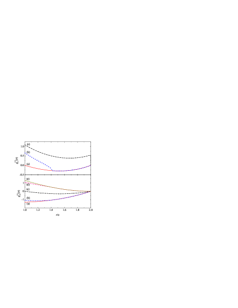
Figure 3: (Top) Plot of $g_{11}^{(1)}(\mathbf{r})$ as a function of $r$ for (a) $\theta=0$ and $\pi$, (b) $\theta=\frac{\pi}{4}$ and $\frac{3\pi}{4}$, and (c) $\theta=\frac{\pi}{2}$. (Bottom) Plot of the regular part of $g_{12}^{(1)}(\mathbf{r})$ as a function of $r$ for (a) $\theta=0$, (b) $\theta=\frac{\pi}{4}$, (c) $\theta=\frac{\pi}{2}$, (d) $\theta=\frac{3\pi}{4}$, and (e) $\theta={\pi}$. The interaction potential is given by Eq. (6) (sketched in Fig. 2), except that the sticky limit with Baxter’s temperature $\tau=0.1$ has been taken (see Sec. IV).

As our aim is to remove the orientational dependence in the original potential altogether, a further simplification is required to reduce the problem to a simple binary mixture having asymmetric correlation functions dependent only on distances and not on orientations of spheres. This will be the orientational average discussed in Sec. III.

III Orientational average and thermodynamics

III.1 Orientational average

Most of the content of this section applies to a mixture (with any number of components) characterized by any anisotropic potential $\phi_{ij}(\mathbf{r})=\phi_{ji}(-\mathbf{r})$ exhibiting the quasi-isotropic form (LABEL:mapping:eq5), where, in general $\varphi_{ij}(r)\neq\varphi_{ji}(r)$ if $i\neq j$. In that case, we note that the thermodynamic quantities will generally involve integrals of the general form

$$I_{ij} = \int d\mathbf{r}\,g_{ij}(\mathbf{r})\mathcal{F}_{ij}(\mathbf{r})$$ (7)

with

$$\mathcal{F}_{ij}\left(\mathbf{r}\right) = {F}_{ij}(r)\Theta\left(\cos\theta\right)+{F}_{ji}(r)\Theta\left(-\cos\theta\right),$$ (8)

where in general $F_{ij}(r)\neq F_{ji}(r)$ if $i\neq j$. This strongly suggests that one can define the two orientational averages $g_{ij}^{+}(r)$ and $g_{ij}^{-}(r)$ as

$$g_{ij}^{+}(r)\equiv\overline{g}_{ij}(r)={\int_{0}^{1}d\left(\cos\theta\right)g_{ij}(\mathbf{r})},$$ (9)

$$g_{ij}^{-}(r)\equiv\overline{g}_{ji}(r)={\int_{-1}^{0}d\left(\cos\theta\right)g_{ij}(\mathbf{r})}.$$ (10)

Note that $g_{ij}^{-}(r)=g_{ji}^{+}(r)$, and this suggests the use of the notation $\overline{g}_{ij}(r)$ and $\overline{g}_{ji}(r)$ instead of $g_{ij}^{+}(r)$ and $g_{ij}^{-}(r)$, respectively. Taking into account Eqs. (8)–(10), Eq. (7) becomes

$$I_{ij} = \frac{1}{2}\int d\mathbf{r}\,\left[\overline{g}_{ij}(r){F}_{ij}\left(r\right)+\overline{g}_{ji}(r){F}_{ji}\left(r\right)\right].$$ (11)

In the case of a double summation over $i$ and $j$,

$$\sum_{i,j}x_{i}x_{j}I_{ij} = \sum_{i,j}x_{i}x_{j}\int d\mathbf{r}\,\overline{g}_{ij}(r){F}_{ij}\left(r\right),$$ (12)

where $x_{i}$ denotes the mole fraction of species $i$.

III.2 Thermodynamics of the mixture: energy, virial, and compressibility routes

We can now particularize the general result (12) to specific cases.

In the case of the internal energy, $\mathcal{F}_{ij}(\mathbf{r})=\phi_{ij}(\mathbf{r})$ and so the energy equation of state can be written asHansen86

$$u_{\text{ex}} = \frac{1}{2}\rho\sum_{i,j}x_{i}x_{j}\int d{\bf r}\,g_{ij}\left(\mathbf{r}\right)\phi_{ij}\left(\mathbf{r}\right)$$ (13)

$$= \frac{1}{2}\rho\sum_{i,j}x_{i}x_{j}\int d{\bf r}\,\overline{y}_{ij}\left(r\right)\varphi_{ij}(r)e^{-\beta\varphi_{ij}(r)},$$

where $u_{\text{ex}}$ is the excess internal energy per particle, $\rho$ is the number density, $\beta=1/k_{B}T$ ($k_{B}$ and $T$ being the Boltzmann constant and the temperature, respectively), and $\overline{y}_{ij}({r})\equiv\overline{g}_{ij}({r})e^{\beta\varphi_{ij}({r})}$ is the orientational average of the cavity function ${y}_{ij}(\mathbf{r})\equiv{g}_{ij}(\mathbf{r})e^{\beta\phi_{ij}(\mathbf{r})}$.

A similar result holds for the virial route to the equation of state,

$$Z \equiv \frac{P}{\rho k_{B}T}$$ (14)

$$= 1+\frac{1}{6}\rho\sum_{i,j}x_{i}x_{j}\int d\mathbf{r}\,y_{ij}\left(\mathbf{r}\right)\mathbf{r}\cdot\nabla e^{-\beta\phi_{ij}\left(\mathbf{r}\right)},$$

where $P$ is the pressure. First, note that

$$\nabla\phi_{ij}\left(\mathbf{r}\right) = \left[\frac{d\varphi_{ij}\left(r\right)}{dr}\Theta\left(\cos\theta\right)+\frac{d\varphi_{ji}\left(r\right)}{dr}\Theta\left(-\cos\theta\right)\right]\widehat{\mathbf{r}}$$ (15)

$$-\delta\left(z\right)\left[\varphi_{ij}\left(r\right)-\varphi_{ji}\left(r\right)\right]\widehat{\mathbf{z}}.$$

Therefore,

$$\mathbf{r}\cdot\nabla\phi_{ij}(\mathbf{r})=r\left[\frac{d\varphi_{ij}(r)}{dr}\Theta(\cos\theta)+\frac{d\varphi_{ji}(r)}{dr}\Theta(-\cos\theta)\right],$$

and thus

$$Z=1+\frac{1}{6}\rho\sum_{i,j}x_{i}x_{j}\int d\mathbf{r}\,\overline{y}_{ij}\left({r}\right){r}\frac{d}{dr}e^{-\beta\varphi_{ij}({r})}.$$ (17)

Finally, let us consider the compressibility route. In a mixture, the (dimensionless) isothermal compressibility $\chi_{T}$ is in general given by

$$\chi_{T}^{-1} = \frac{1}{k_{B}T}\left(\frac{\partial p}{\partial\rho}\right)_{T,\{x_{j}\}}$$ (18)

$$= \sum_{i,j}\sqrt{x_{i}x_{j}}\left[\mathsf{I}+\widehat{\mathsf{h}}\left(0\right)\right]^{-1}_{ij},$$

where $\widehat{h}_{ij}(0)$ is proportional to the zero wavenumber limit of the Fourier transform of the total correlation function $h_{ij}(\mathbf{r})=g_{ij}(\mathbf{r})-1$, namely

$$\widehat{h}_{ij}(0) = \rho\sqrt{x_{i}x_{j}}\int d\mathbf{r}\,h_{ij}\left(\mathbf{r}\right)$$ (19)

$$= \frac{\rho\sqrt{x_{i}x_{j}}}{2}\int d\mathbf{r}\,\left[\overline{h}_{ij}\left({r}\right)+\overline{h}_{ji}\left({r}\right)\right].$$

In the specific case of a binary mixture considered here, Eq. (18) becomes

$$\chi_{T}^{-1}=\frac{1+x_{2}\widehat{h}_{11}(0)+x_{1}\widehat{h}_{22}(0)-2\sqrt{x_{1}x_{2}}\widehat{h}_{12}(0)}{\left[1+\widehat{h}_{11}(0)\right]\left[1+\widehat{h}_{22}(0)\right]-\widehat{h}_{12}^{2}(0)}.$$ (20)

Equations (13), (17), (18), and (19) confirm that the knowledge of the two average quantities $\overline{g}_{ij}(r)$ and $\overline{g}_{ji}(r)$ for each pair $ij$ suffices to determine the thermodynamic quantities. In fact, Eqs. (13), (17), (18), and (19) are formally indistinguishable from those corresponding to mixtures with standard isotropic interactions, except that in our case one generally has $\varphi_{ij}(r)\neq\varphi_{ji}(r)$ and, consequently, $\overline{g}_{ij}(r)\neq\overline{g}_{ji}(r)$.

For future convenience, it is expedient to introduce the Laplace transform of $r\overline{g}_{ij}(r)$:

$$G_{ij}(s) = \int_{0}^{\infty}dr\,e^{-sr}r\overline{g}_{ij}(r).$$ (21)

Its small-$s$ behavior is of the formdeHaro08

$$s^{2}G_{ij}(s) = 1+H_{ij}^{(0)}s^{2}+H_{ij}^{(1)}s^{3}+\cdots,$$ (22)

where

$$H_{ij}^{(n)}\equiv\int_{0}^{\infty}dr\,(-r)^{n}r\overline{h}_{ij}(r).$$ (23)

Thus, Eq. (19) becomes

$$\widehat{h}_{ij}(0)=-2\pi\rho\sqrt{x_{i}x_{j}}\left[H_{ij}^{(1)}+H_{ji}^{(1)}\right].$$ (24)

Note that Eq. (22) implies

$$\lim_{s\to 0}s^{2}G_{ij}(s)=1,$$ (25)

$$\lim_{s\to 0}\frac{s^{2}G_{ij}(s)-1}{s}=0.$$ (26)

IV The sticky limit

The mapping of the Kern–Frenkel potential with fixed patch orientation along the $\pm\widehat{\mathbf{z}}$ axis onto a binary mixture represents a considerable simplification. On the other hand, no approximation is involved in this mapping.

The presence of the original SW interactions for the radial part [see Eq. (3)] makes the analytical treatment of the problem a formidable task. Progresses can however be made by considering the Baxter SHS limit, for which a well defined approximate scheme of solution is available in the isotropic case for both one-componentBaxter68 and multi-component PS75 ; Barboy75 ; Barboy79 ; Zaccarelli00 ; TKR02 fluids. The discussion reported below closely follows the analogue for Baxter symmetric mixtures.Barboy75 ; Barboy79

Let us start by rewriting Eq. (6) as

$$\varphi_{ij}(r)=\left\{\begin{array}[]{ll}\infty,&r<\sigma,\\ -\epsilon_{ij},&\sigma<r<\lambda\sigma,\\ 0,&r>\lambda\sigma,\end{array}\right.$$ (30)

where $\epsilon_{11}=\epsilon_{22}=\epsilon_{21}=0$ and $\epsilon_{12}=\epsilon>0$. However, in this section we will assume generic energy scales $\epsilon_{ij}$. In that case, the virial equation of state (17) becomes

$$Z=1+4\eta\overline{y}(\sigma)-12\eta\sum_{i,j}x_{i}x_{j}{t_{ij}}\frac{\lambda^{3}\overline{y}_{ij}(\lambda\sigma)-\overline{y}_{ij}(\sigma)}{\lambda^{3}-1},$$ (31)

where $\eta\equiv\frac{\pi}{6}\rho\sigma^{3}$ is the packing fraction,

$$\overline{y}(r)=\sum_{i,j}x_{i}x_{j}\overline{y}_{ij}(r)$$ (32)

is the orientational average global cavity function, and

$$t_{ij}\equiv\frac{1}{12\tau_{ij}} \equiv \frac{1}{3}\left(\lambda^{3}-1\right)\left(e^{\beta\epsilon_{ij}}-1\right)$$ (33)

is a parameter measuring the degree of “stickiness” of the SW interaction $\varphi_{ij}(r)$. This parameter will be used later on to connect results from numerical simulations of the actual Janus fluid with analytical results derived for asymmetric SHS mixtures. Although Baxter’s temperature parameters $\tau_{ij}$ are commonly used in the literature, we will employ the inverse temperature parameters $t_{ij}=1/12\tau_{ij}$ in most of the mathematical expressions.

In the case of the interaction potential (30), the energy equation of state (13) reduces to

$$u_{\text{ex}} = -12\frac{\eta}{\sigma^{3}}\sum_{i,j}x_{i}x_{j}\epsilon_{ij}e^{\beta\epsilon_{ij}}\int_{\sigma}^{\lambda\sigma}dr\,r^{2}\overline{y}_{ij}(r).$$ (34)

The compressibility equation of state (18) does not simplify for the SW interaction .

Since the (orientational average) cavity function $\overline{y}_{ij}(r)$ must be continuous, it follows that

$$\overline{g}_{ij}(r)=\overline{y}_{ij}(r)\left[e^{\beta\epsilon_{ij}}\Theta(r-\sigma)-\left(e^{\beta\epsilon_{ij}}-1\right)\Theta(r-\lambda\sigma)\right].$$ (35)

Following Baxter’s prescription,Baxter68 we now consider the SHS limit

$$\lambda\to 1,\quad\epsilon_{ij}\to\infty,\quad t_{ij}\equiv\frac{1}{12\tau_{ij}}\to{(\lambda-1)}{e^{\beta\epsilon_{ij}}}=\text{finite},$$ (36)

so that the well (30) becomes infinitely deep and narrow and can be described by a single (inverse) stickiness parameter $\tau_{ij}$. Note that in the present Janus case ($\epsilon_{11}=\epsilon_{22}=\epsilon_{21}=0$, $\epsilon_{12}=\epsilon>0$) one actually has $t_{11}=t_{22}=t_{21}=0$ and $t_{12}=t=1/12\tau$.

In the SHS limit (36), Eqs. (31), (34), and (35) become, respectively,

$$Z=1+4\eta\overline{y}(\sigma)-4\eta\sum_{i,j}x_{i}x_{j}{t_{ij}}\left[3\overline{y}_{ij}(\sigma)+\sigma\overline{y}_{ij}^{\prime}(\sigma)\right],$$ (37)

$$u_{\text{ex}} = -12{\eta}\sum_{i,j}x_{i}x_{j}\epsilon_{ij}t_{ij}\overline{y}_{ij}(\sigma),$$ (38)

$$\overline{g}_{ij}(r) = \overline{y}_{ij}(r)\left[\Theta(r-\sigma)+{t_{ij}}\sigma\delta_{+}(r-\sigma)\right].$$ (39)

In Eq. (37), $\overline{y}_{ij}^{\prime}(\sigma)$ must be interpreted as $\lim_{\lambda\to 1}\left.\frac{d}{dr}\overline{y}_{ij}(r)\right|_{r=\sigma}$, which in principle differs from $\left.\frac{d}{dr}\lim_{\lambda\to 1}\overline{y}_{ij}(r)\right|_{r=\sigma}$.YS93 However, both quantities coincide in the one-dimensional caseYS93 and are expected to coincide in the three-dimensional case as well. This is just a consequence of the expected continuity of $\frac{d}{dr}\overline{y}_{ij}(r)$ at $r=\lambda\sigma$ in the SW case.A00

Thermodynamic consistency between the virial and energy routes implies

$$\rho\frac{\partial u_{\text{ex}}}{\partial\rho}=\frac{\partial Z}{\partial\beta}=\sum_{i,j}\epsilon_{ij}t_{ij}\frac{\partial Z}{\partial t_{ij}}.$$ (40)

Using Eqs. (37) and (38) and equating the coefficients of $\epsilon_{ij}$ in both sides, the consistency condition (40) yields

$$x_{i}x_{j}\left[\sigma\overline{y}_{ij}^{\prime}(\sigma)-3\eta\frac{\partial\overline{y}_{ij}(\sigma)}{\partial\eta}\right]=\sum_{k,\ell}x_{k}x_{\ell}$$

$$\times\left\{\frac{\partial\overline{y}_{k\ell}(\sigma)}{\partial t_{ij}}-{t_{k\ell}}\frac{\partial}{\partial t_{ij}}\left[3\overline{y}_{k\ell}(\sigma)+\sigma\overline{y}_{k\ell}^{\prime}(\sigma)\right]\right\}.$$ (41)

For distances $r\gtrsim\sigma$, the orientational averages of the cavity functions can be Taylor expanded as

$$\Theta(r-\sigma)\overline{y}_{ij}(r)=\Theta(r-\sigma)\left[\overline{y}_{ij}(\sigma)+\overline{y}_{ij}^{\prime}(\sigma)(r-\sigma)+\cdots\right].$$ (42)

Hence, if we denote by $Y_{ij}(s)$ the Laplace transform of $\Theta(r-\sigma)r\overline{y}_{ij}(r)$, Eq. (42) yields for large $s$

$$e^{\sigma s}sY_{ij}(s)=\sigma\overline{y}_{ij}(\sigma)+\left[\overline{y}_{ij}(\sigma)+\sigma\overline{y}_{ij}^{\prime}(\sigma)\right]s^{-1}+\cdots.$$ (43)

According to Eqs. (39) and (21), the relationship between the Laplace function $G_{ij}(s)$ and $Y_{ij}(s)$ is

$$G_{ij}(s) = Y_{ij}(s)+{\sigma^{2}}t_{ij}\overline{y}_{ij}(\sigma)e^{-\sigma s}.$$ (44)

Inserting Eq. (43) into Eq. (44), we obtain the following large-$s$ behavior of $G_{ij}(s)$:

$$e^{\sigma s}G_{ij}(s) = {\sigma^{2}}t_{ij}\overline{y}_{ij}(\sigma)+\sigma\overline{y}_{ij}(\sigma)s^{-1}$$

$$+\left[\overline{y}_{ij}(\sigma)+\sigma\overline{y}_{ij}^{\prime}(\sigma)\right]s^{-2}+{\cal O}(s^{-3}).$$

A consequence of this is

$$\frac{\lim_{s\to\infty}e^{\sigma s}G_{ij}(s)}{\lim_{s\to\infty}s\left[e^{\sigma s}G_{ij}(s)-\lim_{s\to\infty}e^{\sigma s}G_{ij}(s)\right]}=\sigma t_{ij}.$$ (46)

V A heuristic, non-perturbative analytical theory

V.1 A simple approximate scheme within the Percus–Yevick closure

The Ornstein–Zernike (OZ) equation for an anisotropic mixture readsHansen86

$${h_{ij}(\mathbf{r}_{12})} = {c_{ij}(\mathbf{r}_{12})+\rho\sum_{k}x_{k}\int d\mathbf{r}_{3}\,h_{ik}(\mathbf{r}_{13})c_{kj}(\mathbf{r}_{32})}$$

$$= {c_{ij}(\mathbf{r}_{12})+\rho\sum_{k}x_{k}\int d\mathbf{r}_{3}\,c_{ik}(\mathbf{r}_{13})h_{kj}(\mathbf{r}_{32})},$$

where $c_{ij}(\mathbf{r})$ is the direct correlation function. The PY closure reads

$$c_{ij}(\mathbf{r}) = g_{ij}(\mathbf{r})\left[1-e^{\beta\phi_{ij}(\mathbf{r})}\right].$$ (48)

Introducing the averages $c_{ij}^{+}(r)=\overline{c}_{ij}(r)$ and $c_{ij}^{-}(r)=\overline{c}_{ji}(r)$ for $c_{ij}(\mathbf{r})$ in a way similar to Eqs. (9) and (10), Eq. (48) yields

$$\overline{c}_{ij}({r})=\overline{g}_{ij}({r})\left[1-e^{\beta\varphi_{ij}({r})}\right].$$ (49)

Thus, the PY closure for the full correlation functions $c_{ij}(\mathbf{r})$ and $g_{ij}(\mathbf{r})$ translates into an equivalent relation for the orientational average functions $\overline{c}_{ij}({r})$ and $\overline{g}_{ij}({r})$. A similar reasoning, on the other hand, is not valid for the OZ relation. Multiplying both sides of the first equality in Eq.  (V.1) by $\Theta(\cos\theta_{12})$ and integrating over $\cos\theta_{12}$ one gets

$${\overline{h}_{ij}({r}_{12})} = {\overline{c}_{ij}({r}_{12})+\rho\sum_{k}x_{k}\int d\mathbf{r}_{3}\,\int_{0}^{1}d\left(\cos\theta_{12}\right)}$$ (50)

$$\times{h_{ik}(\mathbf{r}_{13})c_{kj}(\mathbf{r}_{32})}.$$

The same result is obtained if we start from the second equality in Eq.  (V.1), multiply by $\Theta(-\cos\theta_{12})$, integrate over $\cos\theta_{12}$, and make the changes $\mathbf{r}_{12}\to-\mathbf{r}_{12}$, $\mathbf{r}_{13}\to-\mathbf{r}_{13}$, and $i\leftrightarrow j$. Equation (50) shows that in the case of anisotropic potentials of the form (LABEL:mapping:eq5) the OZ equation does not reduce to a closed equation involving the averages $\overline{h}_{ij}({r})$ and $\overline{c}_{ij}({r})$ only, as remarked.

In order to obtain a closed theory, we adopt the heuristic mean-field decoupling approximation

$${\int d\mathbf{r}_{3}\,\int_{0}^{1}d\left(\cos\theta_{12}\right)\,h_{ik}(\mathbf{r}_{13})c_{kj}(\mathbf{r}_{32})}$$

$$\to {\int d\mathbf{r}_{3}\,\overline{h}_{ik}\left({r}_{13}\right)}{\overline{c}_{kj}\left({r}_{32}\right)}.$$ (51)

Under these conditions, the true OZ relation (50) is replaced by the pseudo-OZ relation

$${\overline{h}_{ij}({r}_{12})=\overline{c}_{ij}({r}_{12})+\rho\sum_{k}x_{k}\int d\mathbf{r}_{3}\,\overline{h}_{ik}({r}_{13})\overline{c}_{kj}({r}_{32})}.$$ (52)

This can then be closed by the PY equation (49) and standard theory applies. An alternative and equivalent view is to consider $\overline{c}_{ij}({r})$ not as the orientational average of the true direct correlation function $c_{ij}(\mathbf{r})$ but as exactly defined by Eq. (52). Within this interpretation, Eq. (49) then represents a pseudo-PY closure not derivable from the true PY closure (48).

Within the above interpretation, it is then important to bear in mind that the functions $\overline{g}_{ij}(r)$ obtained from the solution of a combination of Eqs. (49) and (52) are not equivalent to the orientational averages of the functions $g_{ij}(\mathbf{r})$ obtained from the solution of the true PY problem posed by Eqs. (V.1) and complemented by the PY condition (48). As a consequence, the solutions to Eqs. (49) and (52) are not expected to provide the exact $\overline{g}_{ij}(r)$ to first order in $\rho$, in contrast to the true PY problem. This is an interesting nuance that will be further discussed in Sec. V.3.3.

The main advantage of the approximate OZ relation (52) in the case of anisotropic interactions of the form (LABEL:mapping:eq5) is that it allows to transform the obtention of an anisotropic function $g_{ij}(\mathbf{r})$, but symmetric in the sense that $g_{ij}(\mathbf{r})=g_{ji}(-\mathbf{r})$, into the obtention of an isotropic function $\overline{g}_{ij}(r)$, but asymmetric since $\overline{g}_{ij}(r)\neq\overline{g}_{ji}(r)$. In the case of the anisotropic SHS potential defined above, we can exploit the known solution of the PY equation for isotropic SHS mixtures to construct the solution of the set made of Eqs. (49) and (52). This is done in Subsection V.2 by following the RFA methodology.

V.2 RFA method for SHS

Henceforth, for the sake of simplicity, we take $\sigma=1$ as length unit. The aim of this section is to extend the RFA approximation proposed for symmetric SHS mixturesSantos98 ; deHaro08 to the asymmetric case.

We start with the one-component case.YS93 Let us introduce an auxiliary function $F(s)$ related to the Laplace transform $G(s)$ of $rg(r)$ by

$$G(s)=\frac{1}{2\pi}\frac{se^{-s}}{F(s)+\rho e^{-s}}.$$ (53)

The next step is to approximate $F(s)$ by a rational function,

$$F(s)=\frac{S(s)}{L(s)},$$ (54)

with $S(s)=S^{(0)}+S^{(1)}s+S^{(2)}s^{2}+s^{3}$ and

$$L(s)=L^{(0)}+L^{(1)}s+L^{(2)}s^{2}.$$ (55)

Note that $\lim_{s\to\infty}F(s)/s=1/L^{(2)}=\text{finite}$, so that $\lim_{s\to\infty}e^{s}G(s)=\text{finite}$, in agreement with Eq. (IV). Furthermore, Eq. (25) requires $F(s)+\rho e^{-s}=\mathcal{O}(s^{3})$, so that $S^{(0)}=-\rho L^{(0)}$, $S^{(1)}=\rho\left(L^{(0)}-L^{(1)}\right)$, $S^{(2)}=\rho\left(L^{(1)}-\frac{1}{2}L^{(0)}-L^{(2)}\right)$. Taking all of this into account, Eq. (53) can be rewritten as

$$G(s)=\frac{e^{-s}}{2\pi s^{2}}\frac{{L}(s)}{1-A(s)},$$ (56)

where

$$A(s)=\frac{\rho}{s^{3}}\left[(1-e^{-s})L(s)-L^{(0)}s+\left(\frac{1}{2}L^{(0)}-L^{(1)}\right)s^{2}\right].$$ (57)

In the case of a mixture, $G(s)$, $L(s)$, and $A(s)$ become matrices and Eq. (56) is generalized as

$$G_{ij}(s) = \frac{e^{-s}}{2\pi s^{2}}\left(\mathsf{L}(s)\cdot\left[\mathsf{I}-\mathsf{A}(s)\right]^{-1}\right)_{ij},$$ (58)

where $\mathsf{I}$ is the identity matrix and

$$L_{ij}(s) = L_{ij}^{(0)}+L_{ij}^{(1)}s+L_{ij}^{(2)}s^{2},$$ (59)

$$A_{ij}(s) = \rho\frac{x_{i}}{s^{3}}\left[(1-e^{-s})L_{ij}(s)-L_{ij}^{(0)}s\right.$$ (60)

$$\left.+\left(\frac{1}{2}L_{ij}^{(0)}-L_{ij}^{(1)}\right)s^{2}\right].$$

Note that $\lim_{s\to 0}A_{ij}(s)=\text{finite}$, so that $\lim_{s\to 0}s^{2}G_{ij}(s)=\text{finite}\neq 0$ by construction. Analogously, $\lim_{s\rightarrow\infty}e^{s}G_{ij}(s)=\text{finite}$ also by construction.

The coefficients $L_{ij}^{(0)}$, $L_{ij}^{(1)}$, and $L_{ij}^{(2)}$ are determined by enforcing the exact conditions (25), (26), and (46). The details of the derivation are presented in Appendix B and here we present the final results. The coefficients $L_{ij}^{(0)}$ and $L_{ij}^{(1)}$ do not depend upon the first index $i$ and can be expressed as linear functions of the coefficients $\{L_{kj}^{(2)}\}$:

$$L_{ij}^{(0)} = 2\pi\frac{1+2\eta}{(1-\eta)^{2}}-\frac{12\eta}{1-\eta}\sum_{k}x_{k}L_{kj}^{(2)},$$ (61)

$$L_{ij}^{(1)} = 2\pi\frac{1+\eta/2}{(1-\eta)^{2}}-\frac{6\eta}{1-\eta}\sum_{k}x_{k}L_{kj}^{(2)},$$ (62)

and the coefficients $L_{ij}^{(2)}$ obey the closed set of quadratic equations

$$\frac{L_{ij}^{(2)}}{t_{ij}} = 2\pi\frac{1+\eta/2}{(1-\eta)^{2}}-\frac{6\eta}{1-\eta}\sum_{k}x_{k}\left(L_{ik}^{(2)}+L_{kj}^{(2)}\right)$$ (63)

$$+\frac{6}{\pi}\eta\sum_{k}x_{k}L_{ik}^{(2)}L_{kj}^{(2)}.$$

This closes the problem. Once $L_{ij}^{(2)}$ are known, the contact values are given by

$$\overline{y}_{ij}(1) = \frac{L_{ij}^{(2)}}{2\pi t_{ij}}.$$ (64)

Although here we have taken into account that all the diameters are equal ($\sigma_{ij}=\sigma=1$), the above scheme can be easily generalized to the case of different diameters with the additive rule $\sigma_{ij}=(\sigma_{i}+\sigma_{j})/2$. For symmetric interactions (i.e., $t_{ij}=t_{ji}$) one recovers the PY solution of SHS mixtures for any number of components.TKR02 ; Santos98 It is shown in Appendix C that the pair correlation functions $\overline{g}_{ij}(r)$ derived here are indeed the solution to the PY-like problem posed by Eqs. (49) and (52).

V.3 Case of interest: $t_{11}=t_{22}=t_{21}=0$

In the general scheme described by Eqs. (58)–(64), four different stickiness parameters ($t_{11}$, $t_{12}$, $t_{21}$, and $t_{22}$) are in principle possible. With the convention that in $t_{ij}$ the particle of species $i$ is always located below the particle of species $j$, we might consider the simplest possibility of having only one SHS interaction $t_{12}=t=1/12\tau$ and all other HS interactions ($t_{11}=t_{22}=t_{21}=0$), as illustrated in Fig. 2. This is clearly an intermediate case between a full SHS model ($t_{ij}=t=1/12\tau$) and a full HS model ($t_{ij}=0$), with a predominance of repulsive HS interactions with respect to attractive SHS interactions. This is meant to model the intermediate nature of the original anisotropic Kern–Frenkel potential that interpolates between a SW and a HS isotropic potentials upon decreasing the coverage, that is, the fraction of the SW surface patch with respect to the full surface of the sphere.

V.3.1 Structural properties

If $t_{11}=t_{22}=t_{21}=0$, Eq. (63) implies $L_{11}^{(2)}=L_{22}^{(2)}=L_{21}^{(2)}=0$. As a consequence, Eq. (63) for $i=1$ and $j=2$ yields a linear equation for $L_{12}^{(2)}$ whose solution is

$$L_{12}^{(2)}=2\pi\frac{1+\eta/2}{1-\eta}\frac{t}{1-\eta+6\eta t}.$$ (65)

According to Eq. (64),

$$\overline{y}_{12}(1)=\frac{1+\eta/2}{(1-\eta)^{2}}\left(1-\frac{6\eta t}{1-\eta+6\eta t}\right).$$ (66)

Next, Eqs. (61) and (62) yield

$$\frac{L_{11}^{(0)}}{2\pi}=\frac{L_{21}^{(0)}}{2\pi}=\frac{1+2\eta}{(1-\eta)^{2}},$$ (67)

$$\frac{L_{12}^{(0)}}{2\pi}=\frac{L_{22}^{(0)}}{2\pi}=\frac{1+2\eta}{(1-\eta)^{2}}-\frac{12\eta t}{1-\eta}x_{1}{\overline{y}_{12}(1)},$$ (68)

$$\frac{L_{11}^{(1)}}{2\pi}=\frac{L_{21}^{(1)}}{2\pi}=\frac{1+\eta/2}{(1-\eta)^{2}},$$ (69)

$$\frac{L_{12}^{(1)}}{2\pi}=\frac{L_{22}^{(1)}}{2\pi}=\frac{1+\eta/2}{(1-\eta)^{2}}-\frac{6\eta t}{1-\eta}x_{1}{\overline{y}_{12}(1)}.$$ (70)

Once the functions $L_{ij}(s)$ are fully determined, Eq. (58) provides the Laplace transforms $G_{ij}(s)$. From Eq. (44) it follows that $Y_{11}(s)=G_{11}(s)$, $Y_{22}(s)=G_{22}(s)$, $Y_{21}(s)=G_{21}(s)$, and

$$Y_{12}(s)=G_{12}(s)-t\overline{y}_{12}(1)e^{-s}.$$ (71)

A numerical inverse Laplace transform AW92 allows one to obtain $\overline{g}_{11}(r)$, $\overline{g}_{22}(r)$, $\overline{g}_{21}(r)$, and $\overline{y}_{12}(r)$ for any packing fraction $\eta$, stickiness parameter $t=1/12\tau$, and mole fraction $x_{1}$. In what follows, we will omit explicit expressions related to $\overline{g}_{22}(r)$ since they can be readily obtained from $\overline{g}_{11}(r)$ by the exchange $x_{1}\leftrightarrow x_{2}$.

The contact values $\overline{g}_{ij}(1^{+})=\overline{y}_{ij}(1)$ with $(i,j)\neq(1,2)$ cannot be obtained from Eq. (64), unless the associated $t_{ij}$ are first assumed to be nonzero and then the limit $t_{ij}\to 0$ is taken. A more direct method is to realize that, if $t_{ij}=0$, Eq. (IV) gives

$$\overline{g}_{ij}(1^{+})=\lim_{s\to\infty}e^{s}sG_{ij}(s),\quad(i,j)\neq(1,2).$$ (72)

The results are

$$\overline{g}_{11}(1^{+})=\overline{y}_{11}(1)=\frac{1+\eta/2}{(1-\eta)^{2}}-x_{2}\frac{6\eta t}{1-\eta}{\overline{y}_{12}(1)},$$ (73)

$$\overline{g}_{21}(1^{+})=\overline{y}_{21}(1)=\frac{1+\eta/2}{(1-\eta)^{2}},$$ (74)

$$\overline{y}(1)=\frac{1+\eta/2}{(1-\eta)^{2}}\left(1-x_{1}x_{2}\frac{12\eta t}{1-\eta+6\eta t}\right).$$ (75)

It is interesting to note the property $\overline{g}_{11}(1^{+})+\overline{g}_{22}(1^{+})=\overline{y}_{12}(1)+\overline{g}_{21}(1^{+})$.

To obtain the equation of state from the virial route we will need the derivative $\overline{y}_{12}^{\prime}(1)$. Expanding $e^{s}G_{12}(s)$ in powers of $s^{-1}$ and using Eq. (IV), one gets

$$\frac{\overline{y}_{12}^{\prime}(1)}{\overline{y}_{12}(1)} = \frac{\eta}{(1-\eta)^{2}}\left[3t\left(\frac{2-4\eta-7\eta^{2}}{1+\eta/2}+12x_{1}x_{2}\eta\right)\right.$$ (76)

$$\left.-\frac{9}{2}\frac{1-\eta^{2}}{1+\eta/2}\right].$$

V.3.2 Thermodynamic properties

Virial route.

According to Eq. (37),

$$Z^{v} = 1+4\eta\overline{y}(1)-4x_{1}x_{2}\eta t\left[{3\overline{y}_{12}(1)+\overline{y}_{12}^{\prime}(1)}\right]$$

$$= Z_{\text{HS}}^{v}-4x_{1}x_{2}{\eta}t\left[3\frac{1+3\eta}{1-\eta}\overline{y}_{12}(1)+\overline{y}_{12}^{\prime}(1)\right],$$

where the superscript $v$ denotes the virial route and

$$Z_{\text{HS}}^{v}=\frac{1+2\eta+3\eta^{2}}{(1-\eta)^{2}}$$ (78)

is the HS compressibility factor predicted by the virial route in the PY approximation.

Energy route.

From Eq. (38) we have

$$\frac{u_{\text{ex}}}{\epsilon}=-12x_{1}x_{2}\eta t\overline{y}_{12}(1).$$ (79)

The compressibility factor can be obtained from $u_{\text{ex}}$ via the thermodynamic relation (40), which in our case reads

$$\eta\frac{\partial u_{\text{ex}}/\epsilon}{\partial\eta}=\frac{1}{\epsilon}\frac{\partial Z}{\partial\beta}=t\frac{\partial Z}{\partial t}.$$ (80)

Thus, the compressibility factor derived from the energy route is

$$Z^{u} = Z_{\text{HS}}^{u}+\eta\frac{\partial}{\partial\eta}\int_{0}^{t}dt^{\prime}\frac{u_{\text{ex}}(\eta,t^{\prime})/\epsilon}{t^{\prime}}$$

$$= Z_{\text{HS}}^{u}-3x_{1}x_{2}\frac{\eta}{1-\eta}\left[4t\overline{y}_{12}(1)+\frac{\ln\left(1+\frac{6\eta t}{1-\eta}\right)}{1-\eta}\right],$$

where $Z_{\text{HS}}^{u}$ plays the role of an integration constant and thus it can be chosen arbitrarily. It can be shown S05 ; S06 that the energy and the virial routes coincide when the HS system is the limit of a square-shoulder interaction with vanishing shoulder width. From that point of view one should take $Z_{\text{HS}}^{u}=Z_{\text{HS}}^{v}$ in Eq. (LABEL:3.25). On the other hand, a better description is expected from the Carnahan–Starling (CS) equation of state

$$Z_{\text{HS}}^{\text{CS}}=\frac{1+\eta+\eta^{2}-\eta^{3}}{(1-\eta)^{3}}$$ (82)

Henceforth we will take $Z_{\text{HS}}^{u}=Z_{\text{HS}}^{\text{CS}}$.

Compressibility route.

Expanding $s^{2}G_{ij}(s)$ in powers of $s$ it is straightforward to obtain $H_{ij}^{(1)}$ from Eq. (22). This allows one to use Eqs. (20) and (24) to get the inverse susceptibility $\chi_{T}^{-1}$ as

$$\chi_{T}^{-1}=\frac{1+2\eta}{(1-\eta)^{4}}\frac{1+2\eta-24x_{1}x_{2}t\eta(1-\eta)\overline{y}_{12}(1)}{1-x_{1}x_{2}\left[\frac{12t\eta(1+\eta/2)\overline{y}_{12}(1)}{1+2\eta+36x_{1}x_{2}t{\eta^{2}}\overline{y}_{12}(1)}\right]^{2}},$$ (83)

that, for an equimolar mixture $(x_{1}=x_{2}=\frac{1}{2})$, reduces to

$$\chi_{T}^{-1}=\frac{\left[(1-\eta)^{2}(1+2\eta)+3\eta t\left(2+5\eta-\frac{5}{2}\eta^{2}\right)\right]^{2}}{(1-\eta)^{5}(1-\eta+6\eta t)\left[(1-\eta)^{2}+3\eta t(4-\eta)\right]}.$$ (84)

The associated compressibility factor is then

$$Z^{c}=\frac{1}{\eta}\int_{0}^{\eta}d\eta^{\prime}\,\chi_{T}^{-1}(\eta^{\prime}).$$ (85)

The above integral has an analytical solution, but it is too cumbersome to be displayed here.

V.3.3 Low-density expansion

In the standard case of SHS mixtures with symmetric coefficients in the potential parameters, the PY closure is known to reproduce the exact cavity functions to first order in density and thus the third virial coefficient (see Appendix A.2). However, this needs not be the case in the RFA description for the present asymmetric case, as further discussed below. Note that here, “exact” still refers to the simplified problem (orientational average+sticky limit) of Sections III and IV.

The expansion to first order in density of the Laplace transforms $Y_{ij}(s)$ obtained from Eqs. (44), (58)–(60), and (65)–(70) is

$$Y_{ij}(s)=e^{-s}\left(s^{-1}+s^{-2}\right)+Y_{ij}^{(1)}(s)\rho+\cdots,$$ (86)

where the expressions of the first-order coefficients $Y_{ij}^{(1)}(s)$ will be omitted here. Laplace inversion yields

$$\overline{y}_{ij}^{(1)}(r)=\left.\overline{y}_{ij}^{(1)}(r)\right|_{\text{exact}}-\Delta\overline{y}_{ij}^{(1)}(r),$$ (87)

where $\left.y_{ij}^{(1)}(r)\right|_{\text{exact}}$ are the exact first-order functions given by Eqs. (134)–(136) and the deviations $\Delta y_{ij}^{(1)}(r)$ are

$$\Delta\overline{y}_{11}^{(1)}(r)=\Theta(2-r)x_{2}\frac{2t^{2}}{r}\cos^{-1}\frac{r}{2},$$ (88)

$$\Delta\overline{y}_{12}^{(1)}(r)=\Theta(2-r)t\left(2\sqrt{1-r^{2}/4}-r\cos^{-1}\frac{r}{2}\right),$$ (89)

$$\Delta\overline{y}_{21}^{(1)}(r)=-\Delta\overline{y}_{12}^{(1)}(r).$$ (90)

In the case of the global quantity $\overline{y}^{(1)}(r)$ the result is

$$\overline{y}^{(1)}(r)=\left.\overline{y}^{(1)}(r)\right|_{\text{exact}}-\Delta\overline{y}^{(1)}(r),$$ (91)

where $\left.\overline{y}^{(1)}(r)\right|_{\text{exact}}$ is given by Eq. (137) and

$$\Delta\overline{y}^{(1)}(r)=\Theta(2-r)x_{1}x_{2}\frac{2t^{2}}{r}\cos^{-1}\frac{r}{2}.$$ (92)

While the main qualitative features of the exact cavity function are preserved, there exist quantitative differences. The first-order functions $\overline{y}_{11}^{(1)}(r)$, $\overline{y}_{22}^{(1)}(r)$, and $\overline{y}^{(1)}(r)$ predicted by the RFA account for the exact coefficient of $t$ but do not include the exact term of order $t^{2}$ proportional to $r^{-1}\cos^{-1}(r/2)$. In the case of $\overline{y}_{12}^{(1)}(r)$ and $\overline{y}_{21}^{(1)}(r)$ the exact term of order $t$ proportional to $2\sqrt{1-r^{2}/4}-r\cos^{-1}(r/2)$ is lacking. Also, while the combination $\overline{y}_{11}^{(1)}(r)+\overline{y}_{22}^{(1)}(r)-\overline{y}_{12}^{(1)}(r)-\overline{y}_{21}^{(1)}(r)$ vanishes in the RFA, the exact result is proportional to $t^{2}r^{-1}\cos^{-1}(r/2)$. In short, the RFA correctly accounts for the polynomial terms in $\left.y_{ij}^{(1)}(r)\right|_{\text{exact}}$ but misses the non-polynomial terms.

As for the thermodynamic quantities, expansion of Eqs. (LABEL:3.27), (LABEL:3.25), and (85) gives

$$Z^{v} = 1+4\left(1-3{x_{1}x_{2}}t\right)\eta+10\left[1-6{x_{1}x_{2}}t\left(1-\frac{4}{5}t\right)\right]\eta^{2}$$ (93)

$$+\mathcal{O}(\eta^{3}),$$

$$Z^{u} = 1+4\left(1-3{x_{1}x_{2}}t\right)\eta+10\left[1-6{x_{1}x_{2}}t\left(1-\frac{6}{5}t\right)\right]\eta^{2}$$ (94)

$$+\mathcal{O}(\eta^{3}),$$

$$Z^{c} = 1+4\left(1-3{x_{1}x_{2}}t\right)\eta+10\left[1-6{x_{1}x_{2}}t\left(1-\frac{8}{5}t\right)\right]\eta^{2}$$ (95)

$$+\mathcal{O}(\eta^{3}).$$

Comparison with the exact third virial coefficient, Eq. (147), shows that the coefficient of $t^{2}$ is not correct, with the exact factor $4-3\sqrt{3}/\pi\simeq 2.35$ replaced by $2$, $3$, and $4$ in Eqs. (93)–(95), respectively. One consequence is that the virial and energy routes predict the third virial coefficient much better than the compressibility route. A possible improvement is through the interpolation formula

$$Z^{v,u}=\alpha\left(Z^{v}+Z_{\text{HS}}^{\text{CS}}-Z_{\text{HS}}^{v}\right)+(1-\alpha)Z^{u},$$ (96)

where $\alpha=3\sqrt{3}/\pi-1\simeq 0.65$ with the proviso that $Z_{\text{HS}}^{u}=Z_{\text{HS}}^{\text{CS}}$ in Eq. (LABEL:3.25). Equation (96) then reduces to the CS equation of state if $t=0$ and reproduces the exact third virial coefficient when $t\neq 0$.

V.3.4 Phase transition and critical point

In the limit of isotropic interaction ($t_{ij}=t$), our model reduces to the usual SHS Baxter adhesive one-component model. In spite of the fact that the model is, strictly speaking, known to be pathological,Stell91 it displays a critical behavior that was numerically studied in some details by MC techniques.Miller03 ; Miller04 The corresponding binary mixture also displays well defined critical properties that, interestingly, are even free from any pathological behavior. Zaccarelli00 Moreover, the mechanism behind the pathology of the isotropic Baxter model hinges crucially on the geometry of certain close-packed clusters involving 12 or more equal-sized spheres.Stell91 On the other hand, our Janus model, having frozen orientations, cannot sustain those pathological configurations.

Within the PY approximation, the critical behavior of the original one-component Baxter SHS model was studied using the compressibility and virial routes,Baxter68 as well as the energy route,Watts71 in the latter case with the implicit assumption $Z_{\text{HS}}^{u}=Z_{\text{HS}}^{\text{CS}}$. Numerical simulations indicate that the critical point found through the energy route is the closest to numerical simulation results.Miller03 ; Miller04

As the present specific model ( with, $t_{ij}=t\delta_{i1}\delta_{j2}$) is, in some sense, intermediate between the fully isotropic Baxter SHS one-component model (that has a full, albeit peculiar, gas-liquid transition) and the equally isotropic HS model (that, lacking any attractive part in the potential, cannot have any gas-liquid transition), it is then interesting to ask whether in the equimolar case ($x_{1}=x_{2}=\frac{1}{2}$) it still presents a critical gas-liquid transition.

Table 1: Location of the critical point in the RFA, according to different routes.

Route	$\tau_{c}$	$\eta_{c}$	$Z_{c}$
virial, Eq. (LABEL:3.27)	$0.02050$	$0.1941$	$0.3685$
energy, Eq. (LABEL:3.25)	$0.0008606$	$0.2779$	$0.2906$
hybrid virial-energy, Eq. (96)	$0.01504$	$0.1878$	$0.3441$

The answer depends on the route followed to obtain the pressure. As seen from Eq. (84), the compressibility route yields a positive definite $\chi_{T}^{-1}$, so that no critical point is predicted by this route. On the other hand, an analysis of the virial [Eq. (LABEL:3.27)], energy [Eq. (LABEL:3.25) with $Z_{\text{HS}}^{u}=Z_{\text{HS}}^{\text{CS}}$], and hybrid virial-energy [Eq. (96)] equations of state reveals the existence of van der Waals loops with the respective critical points shown in Table 1. The energy route predicts a critical value $\tau_{c}$ about twenty times smaller than the values predicted by the other two routes.

As an illustration, Fig. 4 shows the binodal and a few isotherms, as obtained from the virial route.

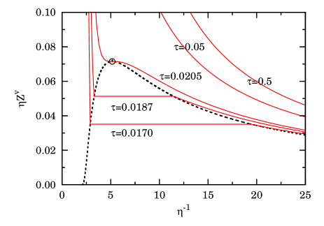
Figure 4: Binodals from the RFA virial route in the equimolar $x_{1}=\frac{1}{2}$ case. The phase diagram is depicted in the $(\eta,\tau)$ plane (solid line, top panel) and in the $(\eta^{-1},\eta Z^{v})$ plane (dashed line, bottom panel). A few characteristic isotherms are plotted in the bottom panel. The critical point is found at $\eta_{c}\simeq 0.1941$, $\tau_{c}\simeq 0.02050$, and $\eta_{c}Z_{c}\simeq 0.07153$ (indicated by a circle in both panels).

V.3.5 A modified approximation

The failure of the RFA to reproduce the exact cavity functions to first order in density (and hence the third virial coefficient) for asymmetric interactions ($t_{ij}\neq t_{ji}$) reveals the price paid for using the orientationally averaged quantities $\overline{g}_{ij}(r)$ instead of the true pair correlation functions ${g}_{ij}(\mathbf{r})$.

A simple way of getting around this drawback for sufficiently low values of both $\eta$ and $t$ consists of modifying the RFA as follows:

$$\overline{y}_{ij}(r)\to\overline{y}_{ij}(r)+\Delta\overline{y}_{ij}^{(1)}(r)\rho,$$ (97)

where the functions $\Delta\overline{y}_{ij}^{(1)}(r)$ are given by Eqs. (88)–(90). We will refer to this as the modified rational-function approximation (mRFA). Note that Eq. (97) implies that $\overline{g}_{ij}(r)\to\overline{g}_{ij}(r)+\Delta\overline{y}_{ij}^{(1)}(r)\rho$, except if $(i,j)=(1,2)$, in which case $\overline{g}_{12}(r)\to\overline{g}_{12}(r)+\Delta\overline{y}_{12}^{(1)}(r)\rho+\Delta\overline{y}_{12}^{(1)}(1)\delta_{+}(r-1)\rho t$.

Since the extra terms in Eq. (97) are proportional to $t$ or $t^{2}$, this modification can produce poor results for sufficiently large stickiness (say, $t\gtrsim 1$) as, for instance, near the critical point.

VI Numerical calculations

VI.1 Details of the simulations

In order to check the theoretical predictions previously reported, we have performed NVT (isochoric-isothermal) MC simulations using the Kern–Frenkel potential defined in Eqs. (LABEL:mapping:eq1)–(4) with a single attractive SW patch (green in the color code of Fig. 1) covering one of the two hemispheres, and with up-down symmetry as depicted in Fig. 2. Particles are then not allowed to rotate around but only to translate rigidly.

The model is completely defined by specifying the relative width $\lambda-1$, the concentration of one species (mole fraction) $x_{1}=1-x_{2}$, the reduced density $\rho^{*}=\rho\sigma^{3}$, and the reduced temperature $T^{*}=k_{B}T/\epsilon$.

In order to make sensible comparison with the RFA theoretical predictions, we have selected the value $\lambda-1=0.05$ as a well width, which is known to be well represented by the SHS limit, Malijevsky06 and use Baxter’s temperature parameter $\tau=\left[4(\lambda^{3}-1)\left(e^{1/T^{*}}-1\right)\right]^{-1}$ [see Eq. (33)] instead of $T^{*}$. It is interesting to note that, while the unconventional phase diagram found in the simulations of Ref. Sciortino10, corresponded to a larger well width ($\lambda=1.5$), the value $\lambda=1.05$ is in fact closer to the experimental conditions of Ref. Hong08, .

During the simulations we have computed the orientational averaged pair correlation functions defined by Eqs. (9) and (10), accumulating separate histograms when $z_{2}-z_{1}>0$ or $z_{1}-z_{2}>0$ in order to distinguish between functions $\overline{g}_{12}(r)=g_{12}^{+}(r)$ and $\overline{g}_{21}(r)=g_{12}^{-}(r)$.

The compressibility factor $Z=\beta P/\rho$ has been evaluated from the values of $\overline{y}_{ij}(r)$ at $r=\sigma$ and $r=\lambda\sigma$ by following Eq. (31) with $t_{ij}=(12\tau)^{-1}\delta_{i1}\delta_{j2}$, and the reduced excess internal energy per particle $u^{*}_{\text{ex}}=u_{\text{ex}}/\epsilon$ has been evaluated directly from simulations.

In all our simulations, we used $N=500$ particles, periodic boundary conditions, an equilibration time of around $10^{5}$ MC steps (where a MC step corresponds to a single particle displacement), and a production time of about $10^{8}$ MC steps for the structure calculations and up to $5\times 10^{8}$ MC steps for the thermophysical calculations. The maximum particle displacement was determined during the first stage of the equilibration run in such a way as to ensure an average acceptance ratio of 50% at production time.

VI.2 Results for non-equimolar binary mixtures

As a preliminary attempt, we consider a binary mixture under non-equimolar conditions, to avoid possible pathologies arising from the symmetry of the two components akin to those occurring in ionic systems. As we shall see below, no such pathologies are found.

In the present case, we consider a system with $x_{1}=1/5$ and $x_{2}=1-x_{1}=4/5$, so that the majority of the spheres have (green) attractive patches pointing in the direction of $-\widehat{\mathbf{z}}$.

A snapshot of an equilibrated configuration is shown in Fig. 5. This configuration was obtained using $N=500$ particles at $\rho^{*}=0.3$ and Baxter temperature $\tau=0.1$ (corresponding to $T^{*}\simeq 0.354$).

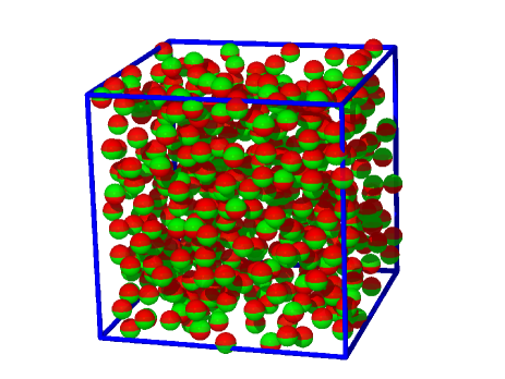
Figure 5: Snapshot of an equilibrated MC simulation under non-equimolar conditions ($x_{1}=1/5$) with Baxter temperature $\tau=0.1$ and density $\rho^{*}=0.3$. In the simulations we used a total number of particles $N=500$.

Note that the above chosen state point ($\rho^{*}=0.3$ and $\tau=0.1$) lies well inside the critical region of the full Baxter SHS adhesive model as obtained from direct MC simulations,Miller03 ; Miller04 although of course the present case is expected to display a different behavior as only a fraction of about $x_{1}x_{2}=4/25$ of the pair contacts are attractive.

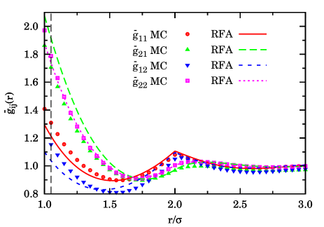
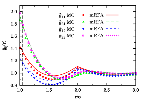
Figure 6: Comparison between MC simulations and the theoretical predictions from RFA (top) and mRFA (bottom) for the orientational averaged distribution functions $\overline{g}_{11}(r)$, $\overline{y}_{12}(r)$, $\overline{g}_{21}(r)$, and $\overline{g}_{22}(r)$ under non-equimolar conditions ($x_{1}=1/5$) at density $\rho^{*}=0.5$ and Baxter temperature $\tau=0.2$. The dashed vertical line indicates the range $r=\lambda=1.05$ of the $(1,2)$ SW interaction used in the simulations. Note that the radial distribution function $\overline{g}_{12}(r)$ is obtained in the MC case by multiplying $\overline{y}_{12}(r)$ in the region $1\leq r\leq\lambda=1.05$ by the factor $e^{1/T^{*}}\simeq 8.93$; in the theoretical cases (SHS limit) $\overline{g}_{12}(r)$ is obtained by adding the singular term $(12\tau)^{-1}\overline{y}_{12}(1)\delta_{+}(r-1)$ to $\overline{y}_{12}(r)$. The error bars on the MC data are within the size of the symbols used.

A good insight on the structural properties of the system can be obtained from the computation of the radial distribution functions $\overline{g}_{11}(r)$, $g_{12}^{+}(r)=\overline{g}_{12}(r)$, $g_{12}^{-}(r)=\overline{g}_{21}(r)$, and $\overline{g}_{22}(r)$. This is reported in Fig. 6 for a state point at density $\rho^{*}=0.5$ and Baxter temperature $\tau=0.2$ (corresponding to $T^{*}\simeq 0.457$). Note that in the case of the pair $(1,2)$ what is actually plotted is the cavity function $\overline{y}_{12}(r)$ rather than $\overline{g}_{12}(r)$, as explained in the caption of Fig. 6.

The relatively low value $\tau=0.2$ gives rise to clearly distinct features of the four MC functions $\overline{g}_{ij}(r)$ (which would collapse to a common HS distribution function in the high-temperature limit $\tau\to\infty$). We observe that $\overline{g}_{22}(r)\simeq\overline{g}_{21}(r)>\overline{g}_{11}(r)>\overline{y}_{12}(r)$ in the region $1\leq r\lesssim 1.5$. Moreover, $\overline{g}_{11}(r)$ and $\overline{g}_{12}(r)$ exhibit a rapid change around $r=2$. This is because when a pair $(1,1)$ is separated a distance $r\approx 2$ there is enough room to fit a particle of species 2 in between and that particle will interact attractively with the particle of the pair $(1,1)$ below it. In the case of the pair $(1,2)$ separated a distance $r\approx 2$, the intermediate particle can be either of species 1 (interacting attractively with the particle of species 2 above it) or of species 2 (interacting attractively with the particle of species 1 below it). The same argument applies to a pair $(2,2)$ separated a distance $r\approx 2$, but in that case the intermediate particle must be of species 1 to produce an attractive interaction; since the concentration of species 1 is four times smaller than that of species 2, the rapid change of $\overline{g}_{22}(r)$ around $r=2$ is much less apparent than that of $\overline{g}_{11}(r)$ and $\overline{g}_{12}(r)$ in Fig. 6. On the other hand, in a pair $(2,1)$ separated a distance $r\approx 2$ an intermediate particle of either species 1 or of species 2 does not create any attraction and thus $\overline{g}_{21}(r)$ is rather smooth at $r=2$. In short, the pair correlation function $\overline{g}_{21}(r)$ exhibits HS-like features, $\overline{g}_{12}(r)$ exhibits SW-like features (very high values in the region $1\leq r\leq\lambda$ and discontinuity at $r=\lambda$ due to the direct SW interaction; rapid change around $r=2$ due to indirect SW interaction), while $\overline{g}_{11}(r)$ and $\overline{g}_{22}(r)$ exhibit intermediate features (rapid change around $r=2$ due to indirect SW interaction).

It is rewarding to notice how well the MC results are reproduced at a semi-quantitative level by the RFA theory (top panel of Fig. 6), in spite of the various approximations involved. In this respect, it is worth recalling that while MC simulations deal with the real Kern–Frenkel potential, albeit with constrained angular orientations, the RFA theory deals with the asymmetric binary mixture resulting from the mapping described in Section II, and this represents an indirect test of the correctness of the procedure. In addition, the RFA does not attempt to describe the true SW interaction (i.e., finite $\lambda-1$ and $T^{*}$) but the SHS limit ($\lambda-1\to 0$ and $T^{*}\to 0$ with finite $\tau$). This limit replaces the high jump of $\overline{g}_{12}(r)$ in the region $1\leq r\leq\lambda$ by a Dirac’s delta at $r=1^{+}$ and the rapid change of $\overline{g}_{12}(r)$, $\overline{g}_{11}(r)$, and $\overline{g}_{22}(r)$ around $r=2$ by a kink. Finally, the RFA worked out in Sec. V.2 results from a heuristic generalization to asymmetric mixtures ($\tau_{ij}\neq\tau_{ji}$) of the PY exact solution for SHS symmetric mixtures ($\tau_{ij}=\tau_{ji}$),PS75 ; Barboy75 ; Barboy79 ; Zaccarelli00 ; TKR02 ; Santos98 but it is not the solution of the PY theory for the asymmetric problem, as discussed in Sec. V.1. As a matter of fact, the top panel of Fig. 6 shows that some of the drawbacks of the RFA observed to first order in density in Sec. V.3.3 [see Eqs. (87)–(90)] remain at finite density: in the region $1\leq r\lesssim 1.5$ the RFA underestimates $\overline{y}_{12}(r)$, $\overline{g}_{11}(r)$, and $\overline{g}_{22}(r)$, while it overestimates $\overline{g}_{21}(r)$. These discrepancies are widely remedied, at least in the region $1\leq r\lesssim 1.25$, by the mRFA approach [see Eq. (97)], as shown in the bottom panel of Fig. 6. In particular, the contact values are well accounted for by the mRFA, as well as the property $\overline{g}_{22}(r)\simeq\overline{g}_{21}(r)$. We have observed that the limitations of the correlation functions $\overline{g}_{ij}(r)$ predicted by the RFA become more important as the density and, especially, the stickiness increase and in those cases the mRFA version does not help much since the correction terms $\Delta\overline{y}_{ij}^{(1)}(r)\rho$, being proportional to $\rho$ and to $t$ or $t^{2}$, become too large.

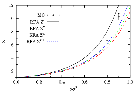
Figure 7: Comparison of MC simulations and RFA theory for the thermodynamics. Both the compressibility factor $Z=\beta P/\rho$ (top) and the excess internal energy per particle $u_{\text{ex}}/\epsilon$ (bottom) are displayed as functions of density for the non-equimolar case $x_{1}=1/5$ and for Baxter temperature $\tau=0.1$. In the case of the compressibility factor (top), results for all four routes (compressibility, virial, energy, and hybrid virial-energy) are reported.

Next we consider thermodynamic quantities, as represented by the compressibility factor $Z=\beta P/\rho$ and the excess internal energy per particle $u_{\text{ex}}/\epsilon$, both directly accessible from NVT numerical MC simulations. These quantities are depicted in Fig. 7 as functions of the reduced density $\rho^{*}$ and for a Baxter temperature $\tau=0.1$. In both cases, the results for the RFA theory are also included. In the case of the compressibility factor, all four routes are displayed: compressibility [Eqs. (66), (83), and (85)], virial [Eqs. (66), (76), and (LABEL:3.27)], energy [Eq. (66) and (LABEL:3.25) with $Z_{\text{HS}}^{u}=Z_{\text{HS}}^{\text{CS}}$], and hybrid virial-energy [Eq. (96)]. In the case of $u_{\text{ex}}/\epsilon$, only the genuine energy route, Eq. (79), is considered. Note that all RFA thermodynamic quantities, including Eq. (85), have explicit analytical expressions.

The top panel of Fig. 7 shows that up to $\rho^{*}\approx 0.7$ the MC data for the compressibility factor are well predicted by the theoretical $Z^{v}$ and, especially, $Z^{u}$ and $Z^{v,u}$. Beyond that point, the numerical results are bracketed by the compressibility route, that overestimates the pressure, and the hybrid virial-energy route, that on the contrary underestimates it. It is interesting to note that, while $Z^{v}<Z^{v,u}<Z^{u}$ to second order in density [cf. Eqs. (93), (94), and (96)], the difference $Z^{v}-Z^{v}_{\text{HS}}$ grows with density more rapidly than the difference $Z^{u}-Z^{u}_{\text{HS}}$ and so both quantities cross at a certain density ($\rho^{*}\simeq 0.567$ if $x_{1}=1/5$ and $\tau=0.1$). Therefore, even though $Z^{v}<Z^{u}$ (because $Z_{\text{HS}}^{v}<Z_{\text{HS}}^{\text{CS}}$), $Z^{v,u}$ is no longer bracketed by $Z^{v}$ and $Z^{u}$ beyond that density ($\rho^{*}\simeq 0.567$ in the case of Fig. 7). On balance, the virial-energy route appears to be the most effective one in reproducing the numerical simulations results of the pressure at $x_{1}=1/5$ and $\tau=0.1$.

As for the internal energy, the bottom panel of Fig. 7 shows that the RFA underestimates its magnitude as a direct consequence of the underestimation of the contact value $\overline{y}_{12}(1)$ [see Eq. (79)]. Although not shown in Fig. 7, we have checked that the internal energy per particle obtained from the virial equation of state (LABEL:3.27) via the thermodynamic relation (80) exhibits a better agreement with the simulation data than the direct energy route.

VI.3 Results for equimolar binary mixtures

Having rationalized the non-equimolar case, the equimolar ($x_{1}=x_{2}=1/2$) case can now be safely tackled. The equimolarity condition makes the system be more akin to the original Janus model (see Fig. 1) since both spin orientations are equally represented.

We start with the snapshot of an equilibrated configuration at density $\rho^{*}=0.3$ and Baxter temperature $\tau=0.1$, that are the same values used in the non-equimolar case. From Fig. 8 it can be visually inspected that, in contrast to the non-equimolar case of Fig. 5, the number of particles with spin up matches that with spin down.

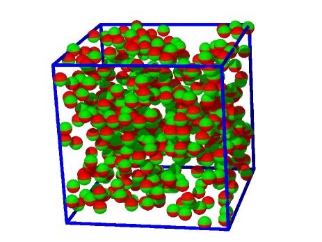
Figure 8: Same as in Fig. 5, but for an equimolar mixture ($x_{1}=x_{2}=1/2$).

This equimolar condition then facilitates the interpretation of the corresponding structural properties, as illustrated by the radial distribution function $\overline{g}_{ij}(r)$ given in Fig. 9.

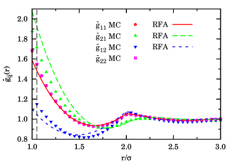
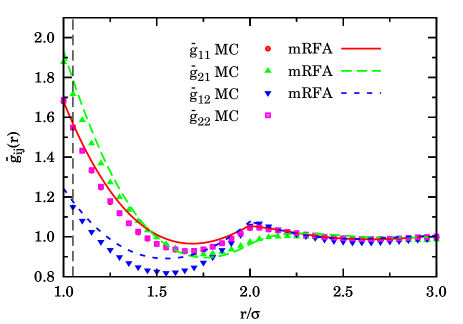
Figure 9: Same as in Fig. 6, but for an equimolar mixture ($x_{1}=x_{2}=1/2$).

This was obtained at a Baxter temperature $\tau=0.2$ and a density $\rho^{*}=0.5$, a state point that is expected to be outside the coexistence curve (see below), but inside the liquid region. Again, this is the same state point as the non-equimolar case previously discussed. Now $\overline{g}_{11}(r)=\overline{g}_{22}(r)$ (independently computed) as it should. Notice that the main features commented before in connection with Fig. 6 persist. In particular, $\overline{g}_{21}(r)>\overline{g}_{11}(r)=\overline{g}_{22}(r)>\overline{y}_{12}(r)$ in the region $1\leq r\lesssim 1.5$, $\overline{g}_{11}(r)=\overline{g}_{22}(r)$ and $\overline{g}_{12}(r)$ present rapid changes around $r=2$, and $\overline{g}_{21}(r)$ exhibits a HS-like shape. Also, as before, the RFA captures quite well the behaviors of the correlation functions (especially noteworthy in the case of $\overline{g}_{11}=\overline{g}_{22}$). On the other hand, the RFA tends to underestimate $\overline{y}_{12}(r)$ and $\overline{g}_{11}(r)=\overline{g}_{22}(r)$ and to overestimate $\overline{g}_{21}(r)$ in the region $1\leq r\lesssim 1.5$. The use of the modified version (mRFA) partially corrects those discrepancies near contact, although the general behavior only improves in the case of $\overline{g}_{21}(r)$.

Comparison between Figs. 6 and 9 shows that $\overline{y}_{12}(r)$ and $\overline{g}_{21}(r)$ are very weakly affected by the change in composition. In fact, the spatial correlations between particles of species 1 and 2 mediated by a third particle (i.e., to first order in density) depend strongly on which particle (1 or 2) is above o below the other one but not on the nature of the third intermediate particle, as made explicit by Eqs.  (135) and (136). Of course, higher-order terms (i.e., two or more intermediate particles) create a composition-dependence on $\overline{y}_{12}(r)$ and $\overline{g}_{21}(r)$, but this effect seems to be rather weak. On the contrary, the minority pair increases its correlation function $\overline{g}_{11}(r)$, while the majority pair decreases its correlation function $\overline{g}_{22}(r)$ in the region $1\leq r\lesssim 1.5$ when the composition becomes more balanced. Again, this can be qualitatively understood by the exact results to first order in density [see Eq. (134)].

VI.4 Preliminary results on the critical behavior

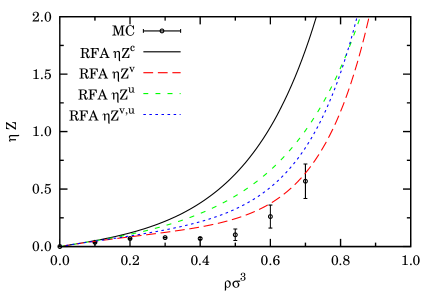
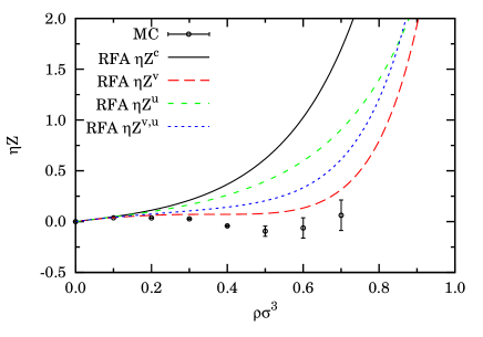
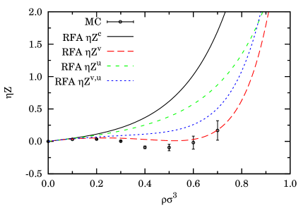
Figure 10: MC simulation data for the scaled pressure $\eta Z=\frac{\pi}{6}\sigma^{3}\beta P$ as a function of $\rho^{*}$ at $\tau=0.030$ (top panel), $0.0205$ (middle panel), and $\tau=0.018$ (bottom panel) in an equimolar mixture. Densities higher than $\rho^{*}=0.7$ are not shown because at these very low temperatures the particles tend to overlap their SW shells and then the calculations slow down considerably. Also shown are the theoretical results for the four routes of the RFA.

One of the most interesting and intriguing predictions of the RFA is the existence of a gas-liquid transition in the equimolar model, despite the fact that only one of the four classes of interactions is attractive (see Sec. V.3.4). The elusiveness of this prediction is reflected by the fact that the compressibility route does not account for a critical point and, although the virial and energy routes do, they widely differ in its location, as seen in Table 1. In this region of very low values of $\tau$ the hybrid virial-energy equation of state is dominated by the virial one and thus the corresponding critical point is not far from the virial value.

A simple heuristic argument can be used to support the existence of a true critical point in our model. According to the Noro–Frenkel (NF) generalized principle of corresponding states,NF00 the critical temperatures of different systems of particles interacting via a hard-core potential plus a short-range attraction are such that the reduced second virial coefficient $B_{2}^{*}=B_{2}/B_{2}^{\text{HS}}$ has a common value $B_{2}^{*c}\simeq-1.21$. In our model, the reduced second virial coefficient is $B_{2}^{*}=1-3t/4=1-1/16\tau$ [see Eq.  (146)]. Thus, assuming the NF ansatz, the critical point would correspond to $\tau_{c}^{\text{NF}}\simeq 0.028$, a value higher than but comparable to that listed in Table 1 from the virial route.

From the computational point of view, a direct assessment on the existence of a gas-liquid transition in the present model is not a straightforward task. Unlike the original SHS Baxter model, a Gibbs ensemble MC (GEMC) calculation for a binary mixture is required to find the coexistence lines. We are currently pursuing this analysis that will be reported elsewhere. As a very preliminary study, we here report NVT results with values of the Baxter temperature close to the critical value $\tau_{c}^{\text{NF}}\simeq 0.028$ expected on the basis of the NF conjecture. More specifically, we have considered $\tau=0.030$, $0.0205$, and $0.018$ (corresponding to $T^{*}\simeq 0.251$, $0.229$, and $0.223$, respectively). The numerical results for the pressure, along with the RFA theoretical predictions, are displayed in Fig. 10.

We observe that at $\tau=0.030$ (top panel) the four theoretical routes clearly indicate a single-phase gas-like behavior with a monotonic increase of the pressure as a function of the density, in consistence with the value $\tau_{c}\simeq 0.0205$ obtained from the RFA virial route. On the other hand, the MC data show a practically constant pressure between $\rho^{*}=0.2$ and $\rho^{*}=0.4$, which is suggestive of $\tau=0.030$ being close to the critical isotherm (remember that $\tau_{c}^{\text{NF}}\simeq 0.028$). The middle panel has been chosen to represent the critical isotherm predicted by the RFA-virial equation of state. In that case, the simulation data present a clear van der Waals loop with even negative pressures around the minimum. A similar behavior is observed at $\tau=0.018$ (bottom panel), except that now the RFA-virial isotherm also presents a visible van der Waals loop. Whereas the observation of negative values of isothermal compressibility in the MC simulations can be attributed to finite-size effects and are expected to disappear in the thermodynamic limit, these preliminary results are highly supportive of the existence of a gas-liquid phase transition in our model with a critical (Baxter) temperature $\tau_{c}\approx 0.03$.

In view of the extremely short-range nature of the potential, the stability of the above liquid phases with respect to the corresponding solid ones may be rightfully questioned.Sciortino10 This is a general issue – present even in the original Baxter model, as well as in the spherically symmetric SW or Yukawa potentials with sufficiently small interaction rangeBHD94 ; LA94 ; HF94 ; MN94 – that is clearly outside the scope of the present manuscript. In any case, it seems reasonable to expect that at sufficiently low temperature and high density the stable phase will consist of an fcc crystal made of layers of alternating species (1-2-1-2-$\cdots$) along the $z$ direction.

VII Conclusions and future perspectives

We have studied thermophysical and structural properties of a Janus fluid having constrained orientations for the attractive hemisphere. The Janus fluid has been modeled using a Kern–Frenkel potential with a single SW patch pointing either up or down, and studied using numerical NVT MC simulations.

The above model has been mapped onto an asymmetric binary mixture where the only memory of the original anisotropic potential stems from the relative position along the $z$-axis of particles of the two species $1$ and $2$. In this way, only one [$(1,2)$ with our choice of labels] out of the four possible interactions is attractive, the other ones [$(1,1)$, $(2,1)$, and $(2,2)$] being simply HS interactions.

In the limit of infinitely short and deep SW interactions (sticky limit), we discussed how a full analytical theory is possible. We developed a new formulation for asymmetric mixtures of the rational-function approximation (RFA), that is equivalent to the PY approximation in the case of symmetric SHS interactions, but differs from it in the asymmetric case. Results from this theory were shown to be in nice agreement with MC simulations using SW interactions of sufficiently short width ($5\%$ of particle size), both for the structural and the thermodynamic properties.

The above agreement is rather remarkable in view of the rather severe approximations involved in the RFA analysis —that are however largely compensated by the possibility of a full analytical treatment— and, more importantly, by the fact that simulations deal with the actual Kern–Frenkel potential with up-down constrained orientations of the patches and SW attractions, while the RFA theory deals with the obtained asymmetric binary mixture and SHS interactions. We regard this agreement as an important indication on the correctness of the mapping.

Within the RFA approximation, all three standard routes to thermodynamics (compressibility, virial, and energy) were considered. To them we added a weighted average of the virial and energy routes with a weight fixed as to reproduce the exact third virial coefficient. Somewhat surprisingly, our results indicate that only the compressibility route fails to display a full critical behavior with a well-defined critical point. The existence of a critical point and a (possibly metastable) gas-liquid phase transition in our model (despite the fact that attractive interactions are partially inhibited) are supported by the NF generalized principle of corresponding statesNF00 and by preliminary simulations results. We plan to carry out more detailed GEMC simulations to fully elucidate this point.

The work presented here can foster further activities toward an analytical theory of the anomalous phase diagram indicated by numerical simulations of the (unconstrained) Janus fluid. We are currently working on the extension of the present model allowing for more general interactions where the red hemispheres in Fig. 2 also present a certain adhesion (e.g., $\tau_{12}<\tau_{11}=\tau_{22}=\tau_{21}<\infty$). This more general model (to which the theory presented in Sec. V.2 still applies) can be continuously tuned from isotropic SHS ($\tau_{ij}=\tau$) to isotropic HS interactions ($\tau_{ij}\to\infty$). The increase in the (Baxter) critical temperatures and densities occurring when equating the stickiness of both hemispheres would then mimic the corresponding increase in the location of the critical point upon an increase of the patch coverage in the Kern–Frenkel model.Sciortino10

Appendix A Exact low-density properties for anisotropic SHS mixtures

A.1 Cavity function to first order in density

To first order in density, the cavity function of an anisotropic mixture is

$$y_{ij}(\mathbf{r})=1+y_{ij}^{(1)}(\mathbf{r})\rho+\mathcal{O}(\rho^{2}),$$ (98)

where

$$y_{ij}^{(1)}(\mathbf{r})=\sum_{k}x_{k}y_{ij;k}^{(1)}(\mathbf{r}),$$ (99)

with

$$y_{ij;k}^{(1)}(\mathbf{r})=\int d\mathbf{r}^{\prime}\,f_{ik}(\mathbf{r}^{\prime})f_{kj}(\mathbf{r}-\mathbf{r}^{\prime}).$$ (100)

Here, ${f_{ij}(\mathbf{r})=e^{-\beta\phi_{ij}(\mathbf{r})}-1}$ is the Mayer function. In the particular case of the anisotropic SHS potential considered in this paper,

$$f_{ij}(\mathbf{r}) = f_{\text{HS}}(r)+\delta(r-1)\left[t_{ij}\Theta(\cos\theta)+t_{ji}\Theta(-\cos\theta)\right]$$ (101)

$$= f_{ji}^{\text{SHS}}(r)+t_{ij}^{-}\delta(r-1)\Theta(\cos\theta),$$

where ${t_{ij}^{-}\equiv t_{ij}-t_{ji},}$

$$f_{\text{HS}}(r)=-\Theta(1-r),\quad f_{ji}^{\text{SHS}}(r)=f_{\text{HS}}(r)+t_{ji}\delta(r-1).$$ (102)

Inserting Eq. (101) into Eq. (100), we get

$$y_{ij;k}^{(1)}(\mathbf{r}) = \Theta(2-r)\left\{\frac{\pi}{12}(2-r)^{2}(4+r)-(t_{ki}+t_{jk})\pi(2-r)\right.$$ (103)

$$+t_{ki}t_{jk}2\pi\left[2\delta(r)+\frac{1}{r}\right]-(t_{ik}^{-}+t_{kj}^{-})\mathcal{A}(\mathbf{r})$$

$$\left.+(t_{ik}^{-}t_{jk}+t_{kj}^{-}t_{ki})\mathcal{L}(\mathbf{r})+t_{ik}^{-}t_{kj}^{-}\mathcal{L}_{0}(\mathbf{r})\right\},$$

where

$$\mathcal{A}(\mathbf{r})\equiv\int d\mathbf{r}^{\prime}\,\delta(r^{\prime}-1)\Theta(1-|\mathbf{r}-\mathbf{r}^{\prime}|)\Theta(z^{\prime}),$$ (104)

$$\mathcal{L}(\mathbf{r})\equiv\int d\mathbf{r}^{\prime}\,\delta(r^{\prime}-1)\delta(|\mathbf{r}-\mathbf{r}^{\prime}|-1)\Theta(z^{\prime}),$$ (105)

$$\mathcal{L}_{0}(\mathbf{r})\equiv\int d\mathbf{r}^{\prime}\,\delta(r^{\prime}-1)\delta(|\mathbf{r}-\mathbf{r}^{\prime}|-1)\Theta(z^{\prime})\Theta(z-z^{\prime}).$$ (106)

It can be proved that

$$\mathcal{A}(\mathbf{r})=\begin{cases}\pi(2-r),&\sqrt{1-r^{2}/4}\leq\cos\theta\leq 1,\\ A(r/2,\theta),&|\cos\theta|\leq\sqrt{1-r^{2}/4},\\ 0,&-1\leq\cos\theta\leq-\sqrt{1-r^{2}/4},\end{cases}$$ (107)

$$\mathcal{L}(\mathbf{r})=\begin{cases}{2\pi}/{r},&\sqrt{1-r^{2}/4}\leq\cos\theta\leq 1,\\ L(r/2,\theta),&|\cos\theta|\leq\sqrt{1-r^{2}/4},\\ 0,&-1\leq\cos\theta\leq-\sqrt{1-r^{2}/4},\end{cases}$$ (108)

$$\mathcal{L}_{0}(\mathbf{r})=\begin{cases}{2\pi}/{r},&\sqrt{1-r^{2}/4}\leq\cos\theta\leq 1,\\ L_{0}(r/2,\theta),&0\leq\cos\theta\leq\sqrt{1-r^{2}/4},\\ 0,&\cos\theta\leq 0,\end{cases}$$ (109)

where

$$A(\ell,\theta) = 2\pi\Theta(\cos\theta)-\pi\ell-2\ell\sin^{-1}\frac{\ell\cos\theta}{\sqrt{1-\ell^{2}}\sin\theta}$$ (110)

$$-2\tan^{-1}\frac{\sqrt{\sin^{2}\theta-\ell^{2}}}{\cos\theta},$$

$$L(\ell,\theta) = -\frac{1}{2\ell}\frac{\partial}{\partial\ell}A(\ell,\theta)$$ (111)

$$= \frac{1}{\ell}\left[\frac{\pi}{2}+\sin^{-1}\frac{\ell\cos\theta}{\sqrt{1-\ell^{2}}\sin\theta}\right],$$

$$L_{0}(\ell,\theta) = L(\ell,\theta)-L(\ell,\pi-\theta)$$ (112)

$$= \frac{2}{\ell}\sin^{-1}\frac{\ell\cos\theta}{\sin\theta\sqrt{1-\ell^{2}}}.$$

In Eqs. (108) and (109) we have omitted terms proportional to $\delta(r)$ since they will not contribute to $g_{ij}(\mathbf{r})$. Note the symmetry relations $\mathcal{A}(\mathbf{r})+\mathcal{A}(-\mathbf{r})=\pi(2-r)$, $\mathcal{L}(\mathbf{r})+\mathcal{L}(-\mathbf{r})=2\pi/r$, $\mathcal{L}(\mathbf{r})-\mathcal{L}(-\mathbf{r})=\mathcal{L}_{0}(\mathbf{r})-\mathcal{L}_{0}(-\mathbf{r})$.

The orientational average

$$\overline{y}_{ij;k}^{(1)}(r)=\int_{0}^{\pi/2}d\theta\,\sin\theta y_{ij;k}^{(1)}(\mathbf{r})$$ (113)

becomes

$$\overline{y}_{ij;k}^{(1)}(r) = \Theta(2-r)\left\{\frac{\pi}{12}(2-r)^{2}(4+r)-(t_{ki}+t_{jk})\pi(2-r)\right.$$ (114)

$$+t_{ki}t_{jk}2\pi\left[2\delta(r)+\frac{1}{r}\right]-(t_{ik}^{-}+t_{kj}^{-})\overline{\mathcal{A}}({r})$$

$$\left.+(t_{ik}^{-}t_{jk}+t_{kj}^{-}t_{ki})\overline{\mathcal{L}}(r)+t_{ik}^{-}t_{kj}^{-}\overline{\mathcal{L}}_{0}(r)\right\},$$

where

$$\overline{\mathcal{A}}({r})=\pi(2-r)\left(1-\sqrt{1-r^{2}/4}\right)+\overline{A}(r/2),$$ (115)

$$\overline{\mathcal{L}}({r})=\frac{2\pi}{r}\left(1-\sqrt{1-r^{2}/4}\right)+\overline{L}(r/2),$$ (116)

$$\overline{\mathcal{L}}_{0}({r})=\frac{2\pi}{r}\left(1-\sqrt{1-r^{2}/4}\right)+\overline{L}_{0}(r/2),$$ (117)

with

$$\overline{A}(\ell) = \int_{\sin^{-1}\ell}^{\pi/2}d\theta\,\sin\theta A(\ell,\theta)$$ (118)

$$= 2\sqrt{1-\ell^{2}}\left(\pi-\pi\ell-1\right)+2\ell\cos^{-1}\ell,$$

$$\overline{L}(\ell) = \int_{\sin^{-1}\ell}^{\pi/2}d\theta\,\sin\theta L(\ell,\theta)$$ (119)

$$= \frac{1}{\ell}\left({\pi}\sqrt{1-\ell^{2}}-\cos^{-1}\ell\right),$$

$$\overline{L}_{0}(\ell) = \int_{\sin^{-1}\ell}^{\pi/2}d\theta\,\sin\theta L_{0}(\ell,\theta)$$ (120)

$$= \frac{1}{\ell}\left({\pi}\sqrt{1-\ell^{2}}-2\cos^{-1}\ell\right).$$

A.2 Second and third virial coefficients

The series expansion of the compressibility factor $Z$ in powers of density defines the virial coefficients:

$$Z=1+B_{2}\rho+B_{3}\rho^{2}+\cdots.$$ (121)

Using Eq. (98) in Eq. (37), one can identify

$$B_{2}=\frac{2\pi}{3}\left(1-3\sum_{i,j}x_{i}x_{j}t_{ij}\right),$$ (122)

$$B_{3}=\frac{2\pi}{3}\sum_{i,j,k}x_{i}x_{j}x_{k}\left[(1-3t_{ij})\overline{y}_{ij;k}^{(1)}(1)-t_{ij}{\overline{y}_{ij;k}^{(1)}}^{\prime}(1)\right].$$ (123)

According to Eq. (114),

$$\overline{y}_{ij;k}^{(1)}(1) = \frac{5\pi}{12}-(t_{ki}+t_{jk})\pi+t_{ki}t_{jk}2\pi-(t_{ik}^{-}+t_{kj}^{-})\overline{\mathcal{A}}({1})$$ (124)

$$+(t_{ik}^{-}t_{jk}+t_{kj}^{-}t_{ki})\overline{\mathcal{L}}(1)+t_{ik}^{-}t_{kj}^{-}\overline{\mathcal{L}}_{0}(1),$$

$${\overline{y}_{ij;k}^{(1)}}^{\prime}(1) = -\frac{3}{4}\pi+(t_{ki}+t_{jk})\pi-t_{ki}t_{jk}2\pi-(t_{ik}^{-}+t_{kj}^{-})\overline{\mathcal{A}}^{\prime}({1})$$ (125)

$$+(t_{ik}^{-}t_{jk}+t_{kj}^{-}t_{ki})\overline{\mathcal{L}}^{\prime}(1)+t_{ik}^{-}t_{kj}^{-}\overline{\mathcal{L}}_{0}^{\prime}(1),$$

where

$$\overline{\mathcal{A}}(1)=\frac{4\pi}{3}-\sqrt{3},\quad\overline{\mathcal{A}}^{\prime}(1)=-\frac{2\pi}{3},$$ (126)

$$\overline{\mathcal{L}}(1)=\frac{4\pi}{3},\quad\overline{\mathcal{L}}^{\prime}(1)=-\frac{2}{3}\left(2\pi-\sqrt{3}\right),$$ (127)

$$\overline{\mathcal{L}}_{0}(1)=\frac{2\pi}{3},\quad\overline{\mathcal{L}}_{0}^{\prime}(1)=-\frac{2}{3}\left(\pi-2\sqrt{3}\right).$$ (128)

The second and third virial coefficients can also be obtained from the compressibility equation (20). To that end, note that

$$\widehat{h}_{ij}(0)=\widehat{h}_{ij}^{(1)}(0)\rho+\widehat{h}_{ij}^{(2)}(0)\rho^{2}+\cdots,$$ (129)

where, according to Eq. (19),

$$\widehat{h}_{ij}^{(1)}(0)=\sqrt{x_{i}x_{j}}2\pi\left(-\frac{2}{3}+t_{ij}+t_{ji}\right),$$ (130)

$$\widehat{h}_{ij}^{(2)}(0) = \sqrt{x_{i}x_{j}}2\pi\Big{\{}t_{ij}\overline{y}_{ij}^{(1)}(1)+t_{ji}\overline{y}_{ji}^{(1)}(1)$$ (131)

$$+\int_{1}^{2}dr\,r^{2}\left[\overline{y}_{ij}^{(1)}(r)+\overline{y}_{ji}^{(1)}(r)\right]\Big{\}}.$$

Inserting this into Eq. (20) and making use of Eqs. (114)–(120), one gets $\chi_{T}^{-1}=1+2B_{2}\rho+3B_{3}\rho^{2}+\cdots$, with $B_{2}$ and $B_{3}$ given by Eqs. (122) and (123), respectively. Furthermore, it can be checked that the exact consistency condition (41) is satisfied by Eqs. (98), (99), (124), and (125). The verification of these two thermodynamic consistency conditions represent stringent tests on the correctness of the results derived in this appendix.

A.3 Case $t_{11}=t_{22}=t_{21}=0$

In the preceding equations of this appendix we have assumed general values for the stickiness parameters $t_{ij}$. On the other hand, significant simplifications occur in our constrained Janus model, where $t_{ij}=t\delta_{i1}\delta_{j2}$. More specifically,

$$y_{11}^{(1)}(\mathbf{r}) = \Theta(2-r)\Big{\{}\frac{\pi}{12}(2-r)^{2}(4+r)-x_{2}t\left[\pi(2-r)\right.$$ (132)

$$\left.-t\mathcal{L}(\mathbf{r})+t\mathcal{L}_{0}(\mathbf{r})\right]\Big{\}},$$

$$y_{12}^{(1)}(\mathbf{r})=\Theta(2-r)\left[\frac{\pi}{12}(2-r)^{2}(4+r)-t\mathcal{A}(\mathbf{r})\right],$$ (133)

$$\overline{y}_{11}^{(1)}(r) = \Theta(2-r)\Big{[}\frac{\pi}{12}(2-r)^{2}(4+r)-x_{2}\pi t\Big{(}2-r$$ (134)

$$-\frac{2t}{\pi r}\cos^{-1}\frac{r}{2}\Big{)}\Big{]},$$

$$\overline{y}_{12}^{(1)}(r) = \Theta(2-r)\left\{\frac{\pi}{12}(2-r)^{2}(4+r)-t\Big{[}\pi(2-r)\right.$$ (135)

$$\left.-2\sqrt{1-r^{2}/4}+r\cos^{-1}\frac{r}{2}\Big{]}\right\},$$

$$\overline{y}_{21}^{(1)}(r) = \Theta(2-r)\Big{\{}\frac{\pi}{12}(2-r)^{2}(4+r)-t\Big{[}2\sqrt{1-r^{2}/4}$$ (136)

$$-r\cos^{-1}\frac{r}{2}\Big{]}\Big{\}},$$

$$\overline{y}^{(1)}(r) = \Theta(2-r)\Big{[}\frac{\pi}{12}(2-r)^{2}(4+r)-x_{1}x_{2}2\pi t\Big{(}2-r$$ (137)

$$-\frac{t}{\pi r}\cos^{-1}\frac{r}{2}\Big{)}\Big{]},$$

$$\overline{y}_{11}^{(1)}(1)=\frac{5\pi}{12}-x_{2}\pi t\left(1-\frac{2t}{3}\right),$$ (138)

$$\overline{y}_{12}^{(1)}(1)=\frac{5\pi}{12}-t\left(\frac{4\pi}{3}-\sqrt{3}\right),$$ (139)

$$\overline{y}_{21}^{(1)}(1)=\frac{5\pi}{12}-t\left(\sqrt{3}-\frac{\pi}{3}\right),$$ (140)

$${\overline{y}_{11}^{(1)}}^{\prime}(1)=-\frac{3\pi}{4}+x_{2}t\left[\pi-\frac{2t}{3}\left(\pi+\sqrt{3}\right)\right],$$ (141)

$${\overline{y}_{12}^{(1)}}^{\prime}(1)=-\frac{3\pi}{4}+t\frac{2\pi}{3},$$ (142)

$${\overline{y}_{21}^{(1)}}^{\prime}(1)=-\frac{3\pi}{4}+t\frac{\pi}{3},$$ (143)

$$\overline{y}^{(1)}(1)=\frac{5\pi}{12}-x_{1}x_{2}2\pi t\left(1-\frac{t}{3}\right),$$ (144)

$${\overline{y}^{(1)}}^{\prime}(1)=-\frac{3\pi}{4}+x_{1}x_{2}2t\left[\pi-\frac{t}{3}\left(\pi+\sqrt{3}\right)\right],$$ (145)

$$\frac{6}{\pi}B_{2}=4\left(1-3x_{1}x_{2}t\right),$$ (146)

$$\left(\frac{6}{\pi}\right)^{2}B_{3}=10\left\{1-6x_{1}x_{2}t\left[1-\frac{2}{5}\left(4-3\frac{\sqrt{3}}{\pi}\right)t\right]\right\},$$ (147)

$$\frac{u_{\text{ex}}}{\epsilon} = -12\eta x_{1}x_{2}t\left\{1+\frac{5}{2}\left[1-\frac{4}{5}\left(4-3\frac{\sqrt{3}}{\pi}\right)t\right]\eta\right\}$$ (148)

$$+\mathcal{O}(\eta^{2}).$$

Appendix B Evaluation of the coefficients $L_{ij}^{(0)}$, $L_{ij}^{(1)}$, and $L_{ij}^{(2)}$

In order to apply Eqs. (25) and (26), it is convenient to rewrite Eq. (58) as

$$\frac{1}{2\pi}\mathsf{L}(s) = \mathsf{Q}(s)\cdot\left[\mathsf{I}-\mathsf{A}(s)\right],$$ (149)

where we have introduced the matrix $\mathsf{Q}$ as

$$Q_{ij}(s) \equiv e^{s}s^{2}G_{ij}(s).$$ (150)

Thus, Eqs. (25) and (26) are equivalent to

$$Q_{ij}(s) = 1+s+\mathcal{O}(s^{2}).$$ (151)

Expanding $A_{ij}(s)$ in powers of $s$ and inserting the result into Eq. (149), one gets

$$\frac{1}{2\pi}L_{ij}^{(0)} = 1-\sum_{k}A_{kj}^{(0)},$$ (152)

$$\frac{1}{2\pi}L_{ij}^{(1)} = 1-\sum_{k}\left(A_{kj}^{(1)}+A_{kj}^{(0)}\right),$$ (153)

where

$$A_{ij}^{(n)}=(-1)^{n}\rho x_{i}\left[\frac{L_{ij}^{(0)}}{(n+3)!}-\frac{L_{ij}^{(1)}}{(n+2)!}+\frac{L_{ij}^{(2)}}{(n+1)!}\right].$$ (154)

Equations (152) and (153) constitute a linear set of equations which allow us to express the coefficients $L_{ij}^{(0)}$ and $L_{ij}^{(1)}$ in terms of the coefficients $\{L_{kj}^{(2)}\}$. The result is given by Eqs. (61) and (62).

It now remains the determination of $L_{ij}^{(2)}$. This is done by application of Eq. (46), i.e., the ratio first term to second term in the expansion of $e^{s}G_{ij}(s)$ for large $s$ must be exactly equal to $t_{ij}$. This is the only point where the stickiness parameters of the mixture appear explicitly.

The large-$s$ behavior from Eq. (58) is

$$2\pi e^{s}G_{ij}(s)=L_{ij}^{(2)}+\left[L_{ij}^{(1)}+\left({\sf L}^{(2)}\cdot{\sf D}\right)_{ij}\right]s^{-1}+{\cal O}(s^{-2}),$$ (155)

where

$$D_{ij} \equiv \rho x_{i}\left(\frac{1}{2}L_{ij}^{(0)}-L_{ij}^{(1)}+L_{ij}^{(2)}\right)$$ (156)

$$= \rho x_{i}\left(L_{ij}^{(2)}-\frac{\pi}{1-\eta}\right).$$

Comparison of Eq. (IV) with Eq. (155) yields Eq. (64) and

$$\frac{12\tau_{ij}L_{ij}^{(2)}}{\sigma_{ij}} = L_{ij}^{(1)}+\sum_{k=1}^{m}L_{ik}^{(2)}D_{kj}.$$ (157)

$$\frac{L_{ij}^{(2)}}{t_{ij}} = L_{ij}^{(1)}+\sum_{k}L_{ik}^{(2)}D_{kj}.$$ (158)

Taking into account Eqs. (62) and (156), Eq. (158) becomes Eq. (63).

Appendix C Recovery of the pseudo-PY solution

The aim of this appendix is to prove that the pair correlation functions $\overline{g}_{ij}(r)$ obtained from the RFA method in Sec. V.2 satisfy Eqs. (49) and (52).

First, note that the pseudo-OZ relation (52) can be rewritten in the form

$$\widehat{\overline{\mathsf{c}}}(q)=\widehat{\overline{\mathsf{h}}}(q)\cdot\left[\mathsf{I}+\widehat{\overline{\mathsf{h}}}(q)\right]^{-1},$$ (159)

where $\mathsf{I}$ is the unit matrix and

$$\widehat{\overline{c}}_{ij}(q)=\rho\sqrt{x_{i}x_{j}}\int d\mathbf{r}\,e^{-i\mathbf{q}\cdot\mathbf{r}}\overline{c}_{ij}(r),$$ (160)

$$\widehat{\overline{h}}_{ij}(q)=\rho\sqrt{x_{i}x_{j}}\int d\mathbf{r}\,e^{-i\mathbf{q}\cdot\mathbf{r}}\overline{h}_{ij}(r).$$ (161)

Note that $\widehat{h}_{ij}(0)=\frac{1}{2}\left[\widehat{\overline{h}}_{ij}(0)+\widehat{\overline{h}}_{ji}(0)\right]$, where $\widehat{h}_{ij}(0)$ is defined by Eq. (19).

The Fourier transform $\widehat{\overline{h}}_{ij}(q)$ of the (orientational average) total correlation function $\overline{h}_{ij}(r)=\overline{g}_{ij}(r)-1$ is related to the Laplace transform $G_{ij}(s)$ [see Eq. (21)] by

$$\widehat{\overline{h}}_{ij}(q)=-2\pi\rho\sqrt{x_{i}x_{j}}\left[\frac{G_{ij}(s)-G_{ij}(-s)}{s}\right]_{s=iq}.$$ (162)

Making use of Eqs.  (58)–(60), it is possible to obtain, after some algebra,

$$\frac{\widehat{\overline{c}}_{ij}(q)}{\rho\sqrt{x_{i}x_{j}}} = \frac{4\pi}{q^{3}}C_{ij}^{(0)}\left(\sin q-q\cos q\right)+\frac{4\pi}{q^{4}}C_{ij}^{(1)}\left[2q\sin q\right.$$ (163)

$$\left.-2-\left(q^{2}-2\right)\cos q\right]+\frac{4\pi}{q^{6}}C_{ij}^{(3)}\left[4q\left(q^{2}-6\right)\right.$$

$$\left.\times\sin q+24-\left(24-12q^{2}+q^{4}\right)\cos q\right]$$

$$+4\pi t_{ij}{y_{ij}(1)}\frac{\sin q}{q},$$

where the coefficients $C_{ij}^{(0)}$, $C_{ij}^{(1)}$, and $C_{ij}^{(3)}$ are independent of $q$ but depend on the density, the composition, and the stickiness parameters. Fourier inversion yields

$$\overline{c}_{ij}(r) = \left[C_{ij}^{(0)}+C_{ij}^{(1)}r+C_{ij}^{(3)}r^{3}\right]\Theta(1-r)$$ (164)

$$+{y_{ij}(1)}t_{ij}\delta_{+}(r-1).$$

Taking into account Eq. (39) we see that Eq. (164) has the structure

$$\overline{c}_{ij}(r)=\overline{g}_{ij}(r)-\overline{y}_{ij}(r).$$ (165)

But this is not but the PY closure relation (49). In passing, we get the cavity function inside the core:

$$y_{ij}(r)\Theta(1-r)=-\left[C_{ij}^{(0)}+C_{ij}^{(1)}r+C_{ij}^{(3)}r^{3}\right]\Theta(1-r).$$ (166)

References

• (1) A. B. Pawar and I. Kretzschmar, Macromol. Rapid Comm. 31, 150 (2010).
• (2) A. Walther and H. E. Müller, Soft Matter 4, 663 (2008).
• (3) L. Hong, A. Cacciuto, E. Luijten, and S. Granick, Langmuir 24, 621 (2008).
• (4) E. Bianchi, R. Blaak, and C. N. Likos, Phys. Chem. Chem. Phys. 13, 6397 (2011).
• (5) Z. L. Zhang and S. C. Glotzer, Nano Lett. 4, 1407 (2004).
• (6) N. Kern and D. Frenkel, J. Chem. Phys. 118, 9882 (2003).
• (7) F. Sciortino, A. Giacometti, and G. Pastore, Phys. Chem. Chem. Phys. 12, 11869 (2010).
• (8) A. Giacometti, F. Lado, J. Largo, G. Pastore, and F. Sciortino, J. Chem. Phys. 131, 174114 (2009).
• (9) A. Giacometti, F. Lado, J. Largo, G. Pastore, and F. Sciortino, J. Chem. Phys. 132, 174110 (2010).
• (10) F. Sciortino, A. Giacometti, and G. Pastore, Phys. Rev. Lett. 103 , 237801 (2009).
• (11) A. Reinhardt, A. J. Williamson, J. P. K. Doyle, J. Carrete, L. M. Varela, and A. A. Louis, J. Chem. Phys. 134, 104905 (2011).
• (12) R. Fantoni, A. Giacometti, F. Sciortino, and G. Pastore, Soft Matter 7, 2419 (2011).
• (13) R. Fantoni, Eur. Phys. J. B 85, 108 (2012).
• (14) R. Zwanzig, J. Chem. Phys. 39, 1714 (1963).
• (15) R. J. Baxter, J. Chem. Phys. 49, 2770 (1968).
• (16) J. P. Hansen and I. R. McDonald, Theory of Simple Liquids (Academic, New York, 1986).
• (17) R. O. Watts, D. Henderson, and R. J. Baxter, Adv. Chem. Phys. 21, 421 (1971).
• (18) J. W. Perram and E. R. Smith, Chem. Phys. Lett. 35, 138 (1975).
• (19) B. Barboy, Chem. Phys. 11, 357 (1975).
• (20) B. Barboy and R. Tenne, Chem. Phys. 38, 369 (1979).
• (21) E. Zaccarelli, G. Foffi, P. Tartaglia, F. Sciortino, and K. A. Dawson, Progr. Colloid Polym. Sci. 115, 371 (2000).
• (22) C. Tutschka, G. Kahl, and E. Riegler, Mol. Phys. 100, 1025 (2002).
• (23) R. Fantoni, D. Gazzillo, A. Giacometti, M. A. Miller, and G. Pastore, J. Chem. Phys. 127, 234507 (2007).
• (24) A. Santos, S. B. Yuste, and M. López de Haro, J. Chem. Phys. 109, 6814 (1998).
• (25) M. López de Haro, S. B. Yuste, and A. Santos, in Theory and Simulations of Hard-Sphere Fluids and Related Systems, Lecture Notes in Physics, vol. 753, A. Mulero, ed. (Springer, Berlin 2008) pp. 183-245.
• (26) S. B. Yuste and A. Santos, Phys. Rev. E 48, 4599 (1993).
• (27) L. Acedo, J. Stat. Phys. 99, 707 (2000).
• (28) J. Abate and W. Whitt, Queueing Systems 10, 5 (1992).
• (29) A. Santos, J. Chem. Phys. 123, 104102 (2005).
• (30) A. Santos, Mol. Phys. 104, 3411 (2006).
• (31) G. Stell, J. Stat. Phys. 63, 1203 (1991).
• (32) M. A. Miller and D. Frenkel, Phys. Rev. Lett. 90, 135702 (2003).
• (33) M. A. Miller and D. Frenkel, J. Chem. Phys. 121, 535 (2004).
• (34) A. Malijevský, S. B. Yuste, and A. Santos, J. Chem. Phys. 125, 074507 (2006).
• (35) M. G. Noro and D. Frenkel, J. Chem. Phys. 113, 2941 (2000).
• (36) P. Bolhuis, M. Hagen, and D. Frenkel, Phys. Rev. E 50, 4880 (1994).
• (37) E. Lomba and N. G. Almarza, J. Chem. Phys. 100, 8367 (1994).
• (38) M. H. J. Hagen and D. Frenkel, J. Chem. Phys. 101, 4093 (1994).
• (39) L. Mederos and G. Navascués, J. Chem. Phys. 101, 9841 (1994).