Linking two consecutive non-merging magnetic clouds with their solar sources
Abstract
On May 15, 2005, a huge interplanetary coronal mass ejection (ICME) was observed near Earth. It triggered one of the most intense geomagnetic storms of solar cycle 23 ( = -263 nT). This structure has been associated with the two-ribbon flare, filament eruption and CME originating in active region (AR) 10759 (NOAA number). We analyze here the sequence of events, from solar wind measurements (at 1 AU) and back to the Sun, to understand the origin and evolution of this geoeffective ICME. From a detailed observational study of in situ magnetic field observations and plasma parameters in the interplanetary (IP) medium, and the use of appropriate models, we propose an alternative interpretation of the IP observations, different to those discussed in previous studies. In our view, the IP structure is formed by two extremely close consecutive magnetic clouds (MCs) that preserve their identity during their propagation through the interplanetary medium. Consequently, we identify two solar events in H and EUV which occurred in the source region of the MCs. The timing between solar and IP events, as well as the orientation of the MC axes and their associated solar arcades are in good agreement. Additionally, interplanetary radio type II observations allow the tracking of the multiple structure through inner heliosphere and to pin down the interaction region to be located midway between the Sun and the Earth. The chain of observations from the photosphere to interplanetary space is in agreement with this scenario. Our analysis allows the detection of the solar sources of the transients and explains the extremely fast changes of the solar wind due to the transport of two attached —though non-merging— MCs which affect the magnetosphere.
DASSO ET AL. \titlerunningheadTRACKING TWO CONSECUTIVE MAGNETIC CLOUDS \setkeysGindraft=false
1 Introduction
Coronal mass ejections (CMEs) remove plasma and magnetic field from the Sun expelling them into interplanetary space. When they are detected in the interplanetary (IP) medium, they are called interplanetary coronal mass ejections (ICMEs). The transit time of an ICME from the Sun to 1 AU is typically in the interval 1 to 5 days (Gopalswamy et al., 2000, 2001a; Rust et al., 2005). A subset of ICMEs, called magnetic clouds (MCs), are characterized by an enhanced magnetic field strength, a smooth and large rotation of the magnetic field vector, and low proton temperature (Burlaga et al., 1981). Fast and large magnetic clouds are mostly observed at 1 AU in the declining phase of a solar cycle, as it happened in the last one during 2003-2005 (e.g., Culhane and Siscoe, 2007).
Interplanetary type II bursts permit the tracking of fast ICMEs through the analysis of radio emission frequency drift (Reiner et al., 1998, 2007; Hoang et al., 2007). Assuming the type II emission to be produced at the fundamental or second harmonic of the local plasma frequency, and with help of a heliospheric density model, the radio frequency can be converted to radial distance. This method has still limitations and allows for possible different interpretations due to the patchiness and the frequency range of the observed radio emissions. The evolution of an ICME can also be followed along its journey using a combination of solar and IP observations together with the results of numerical simulations (e.g., Wu et al., 1999).
Coronal mass ejections are frequently associated with filament eruptions. The directions of the MC axes are found to be roughly aligned with the disappearing filaments (Bothmer and Schwenn, 1994, 1998), preserving their helicity sign. This result has been found for some individual cases by Marubashi (1997); Yurchyshyn et al. (2001); Ruzmaikin et al. (2003); Yurchyshyn et al. (2005); Rodriguez L. et al. (2008). Some quantitative (quantifying magnetic fluxes and helicities) studies of MCs and their solar sources have been also done (Mandrini et al., 2005; Luoni et al., 2005; Longcope et al., 2007). But again, it is not so easy to quantify this association and further developments are needed to really understand the fundamental transport mechanisms and interaction with the ambient solar wind (see, e.g., the review by Démoulin (2008)).
Furthermore, when multiple CMEs are expelled from the Sun, they can be merged leading to the so-called “CME cannibalism” (Gopalswamy et al., 2001b), mainly as a consequence of magnetic reconnection. The interaction of two CMEs in favorable conditions for reconnection has been studied by Wang et al. (2005). However, from a theoretical point of view, two original structures can be preserved with an appropriate orientation of the ejected flux rope (yielding almost parallel interacting magnetic fields). For example, in the MHD simulations of Xiong et al. (2007) the two interacting flux ropes preserved their identity while evolving in the IP medium until they reach the Earth environment or even beyond.
In the magnetohydrodynamic (MHD) framework, a magnetic cloud configuration in equilibrium can be obtained from the balance between the magnetic Lorentz force and the plasma pressure gradient. Several magnetostatic models have been used to describe the configuration of MCs. Frequently, the magnetic field of MCs has been modeled by the so-called Lundquist’s model (Lundquist, 1950), which considers a static and axially symmetric (cylindrical) linear force-free magnetic configuration neglecting the plasma pressure (e.g., Goldstein, 1983; Burlaga, 1988; Lepping et al., 1990; Lynch et al., 2003; Dasso et al., 2005; Leitner et al., 2007; Xiong et al., 2007). The azimuthal and axial field components of the flux rope in this classical configuration are defined by and , where is the distance to the MC axis, is the Bessel function of the first kind of order , is the strength of the field at the cloud axis, and is a constant associated with the twist of the magnetic field lines. Some other refined models have also been proposed to describe the magnetic structure of clouds (e.g., Hu and Sonnerup, 2001; Vandas and Romashets, 2002; Cid et al., 2002); in particular, some of them consider an elliptical shape (Hidalgo et al., 2002a; Hidalgo, 2003) that allows the description of possible distortions of the structures.
On May 15-17, 2005, the strongly southward interplanetary field (above 40 nT) and the high solar wind velocity (close to 1000 km s-1), observed by the Advanced Composition Explorer (ACE), are the cause of a super geomagnetic storm with a depression of the index reaching -263 nT. The IP structure has the characteristics of a MC. Yurchyshyn et al. (2006) associated this structure with the two-ribbon M8.0 X-ray class flare on May 13 at 16:32 UT in AR 10759, accompanied by a filament eruption and CME. These authors identified a single MC, starting at 00:00 UT on May 15 and ending at 09:00 UT on May 16. An event with different boundaries, much smaller than the one described by Yurchyshyn et al., was identified by R. Lepping (start on May 15 at 05:42 UT and end on May 15 at 22:18 UT). The event was qualified with intermediate fitting quality (quality 2) and had a large impact parameter (catalog at http://lepmfi.gsfc.nasa.gov/mfi/mag_cloud_S1.html).
The solar activity evolution along May 13 has been well described by Yurchyshyn et al. (2006) and, more recently, by Liu et al. (2007). Both papers refer mainly to the M8.0 event and conclude that the eruption of a large sigmoidal structure launches the CME observed by the Large Angle and Spectroscopic Coronagraph (LASCO, Brueckner G. E. et al., 1995) at 17:22 UT.
In this paper, we present a detailed analysis of the solar wind conditions at the Lagrangian L1 point using in situ observations (magnetic field and bulk plasma properties) and propose an alternative interpretation of the IP observations. In our view, the observed ICME is in fact formed by two MCs. Since a single solar event cannot explain the arrival of two MCs at 1 AU, we revisit the evolution and activity of AR 10759 and other regions present in the solar disk. We start searching in the Sun for two possible sources of the clouds, even earlier than May 13. We identify a previous candidate event in H and EUV data same day at 12:54 UT in AR 10759, which was classified as a C1.5 flare in GOES. These two events, the one at 12:54 UT and the one at 16:32 UT, give rise to two two-ribbon flares along different portions of the AR magnetic inversion line. The orientations of the magnetic fields associated to both solar events are in good agreement with the fields observed in their associated MCs.
In Section 2 we analyze the solar wind conditions near Earth; in particular, we derive the orientation of the axis for the two MCs by fitting a model to the observations. In Section 3, we revisit the solar events using ground based and satellite data. In Section 4 we present radio type II remote observations, which let us track the multiple structure through the inner heliosphere. Finally, in Section 5, we describe the most plausible physical scenario behind the chain of events from May 13 to 17, 2005, and we give our conclusions.
2 A Large Interplanetary Coronal Mass Ejection: May 15-17.
2.1 In situ plasma and magnetic field observations
The solar wind data were obtained by ACE, located at the Lagrangian point L1. The magnetic field observations come from the Magnetic Fields Experiment (MAG) (Smith et al., 1998) and the plasma data from the Solar Wind Electron Proton Alpha Monitor (SWEPAM) (McComas et al., 1998).
Figure 1 shows the magnetic field (in the Geocentric Solar Ecliptic, GSE, system) and plasma conditions in the solar wind for the long-lasting studied event (00:00 UT on May 15 to 16:00 UT on May 17, 2005), and the consequent magnetospheric activity ( index).
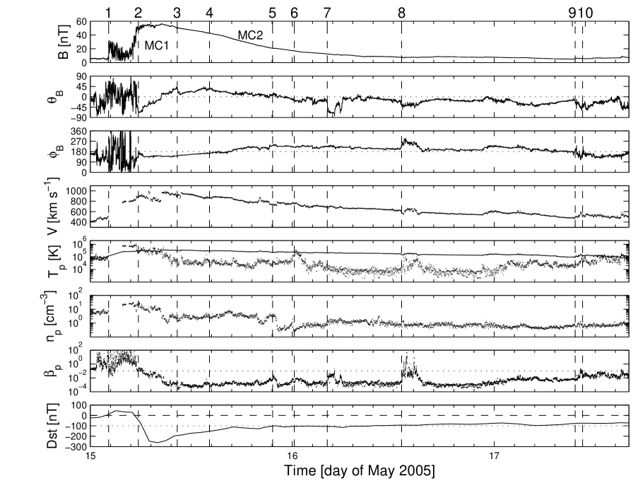
The data in Figure 1 show several features consistent with the presence of ICMEs/MCs: low proton plasma beta, proton temperature lower than expected () for a typical solar wind at a given observed bulk velocity (Lopez, 1987), an almost linear velocity profile, and a smoothly varying magnetic field orientation of high intensity. In particular, from vertical dashed line ’1’ to ’10’ (for timings of tick numbers see next paragraphs and Table 1) the magnetic field intensity is strongly enhanced, although the scale needed to show the whole event in one plot does not allow to observe this enhancement at the end of the time interval. The temporal length of the event is quite large, so that it corresponds to a very extended region, AU, one of the largest ICMEs ever observed (see, e.g., Table 1 of Liu et al. (2005) and Figure 1 of Liu et al. (2006a)). At ’10’, the magnetic field recovers its background value of nT.
From a comparative study between magnetic clouds and complex ejecta, Burlaga et al. (2001) found that while most of the clouds were associated with single solar sources, nearly all the complex ejecta could have had multiple sources. Evidence was also found indicating that long duration complex merged interaction regions (with radial extents of AUs) can be produced by the interaction of two or more CMEs/MCs/shocks (Burlaga et al., 2001, 2003).
In front of the ICME, from 00:00 UT to 02:11 UT on May 15 (labeled as ’1’), the solar wind presents typical conditions with a value of 6 nT, an increasing velocity profile (starting at 400 km s-1 and reaching 500 km s-1), observed proton temperature similar to that expected one () for a typical solar at same velocity, an increasing proton density profile from 3 to 10 protons per cm3, high values of proton plasma (reaching 10-100), and values of the index () corresponding to relatively quiet ring current conditions.
| Tick number | Timing | Substructure |
|---|---|---|
| 1 | 15,02:11 | |
| sheath | ||
| 2 | 15,05:42 | |
| MC1 | ||
| 3 | 15,10:20 | |
| back1 | ||
| 4 | 15,14:10 | |
| MC2 | ||
| 5 | 15,21:40 | |
| MC2 | ||
| 6 | 16,00:15 | |
| MC2 | ||
| 7 | 16,04:10 | |
| back2 | ||
| 8 | 16,13:00 | |
| back2 | ||
| 9 | 17,09:37 | |
| back2 | ||
| 10 | 17,10:30 |
Observations at ’1’ suggest the existence of a strong leading edge shock (not fully confirmed from observations of because of a gap in plasma data from 02:11 UT to 03:50 UT on May 15). Just behind the shock, from ’1’ to ’2’, a typical ICME sheath is present (e.g., high level of fluctuations in , enhanced B strength, high mass density, high ).
A structure with a very high (50-60 nT), one of the highest values ever observed in the solar wind at 1 AU, is found between ’2’ and ’3’. In this range of time, a large scale coherent rotation of the magnetic field vector is present, with going from south to north (see panel). This is a left handed SEN flux rope in the classification of Bothmer and Schwenn (1998). Note the presence of a sudden change of the sense of rotation together with a magnetic discontinuity (MD) at ’3’ (clearly observed in ). A current sheet (i.e., a discontinuity in the observed time series of the magnetic field vector) is expected to be present at the interface that separates two magnetic regions with different magnetic connectivity, i.e., with different magnetic stress. Thus, we interprete the discontinuity at ’3’ as the signature of the end of a first substructure inside the large ICME. This substructure ’2-3’ has also specific physical properties: there are no signatures of expansion (the profile of does not show a significant slope), and the observed temperature decreases in time (hotter near the sheath and colder near substructure ’3-4’). As a consequence of the decreasing profile, values of also decrease, being near ’2’ and reaching values as low as near ’3’. Thus, the substructure ’2-3’ presents some MC signatures (low , coherent rotation of the magnetic field vector) but not all ICMEs features (e.g., is not significantly lower than ). This MC presents a short temporal duration with a spatial size along the Sun-Earth direction of 0.09 AU (4 hs multiplied by 900 km s-1). We interpret the short duration of the first MC as due to the compression made by MC2 at its trailing edge; it is expected that the expansion rate (and the consequent cooling) of the first cloud diminished during part of its journey, where the second MC is pushing it from behind (Wang et al., 2003), consistently with observations ().
After the MD at ’3’, continues increasing up to ’4’, where there is another (weaker, but significant) MD. The region from ’3’ to ’4’ shows the characteristics of the back of flux ropes, previously found by Dasso et al. (2006) in a significantly large non-expanding magnetic cloud (Oct. 1995) and by Dasso et al. (2007) in another huge magnetic cloud (Nov. 2004) in strong expansion. The formation of this back feature is a consequence of previous magnetic reconnection between the front of the flux rope and its environment; magnetic flux is removed from the flux rope front (the front is peeled) while its counterpart in the rear part still remains (Figure 6 of Dasso et al. (2006)). The formation of a back in fast ICMEs is also supported by numerical simulations (see Figure 4 of Wu et al. (2005)).
At the difference of previously studied MC-backs, the region from ’3’ to ’4’ is compressed by the second MC. This region of interaction does not have the same characteristics as corotating interaction regions (CIRs, e.g. Pizzo, 1994) or typical merged interaction regions (MIRs, e.g. Burlaga and Ness, 1993, and references there in). CIRs are due to a fast SW overtaking a slow SW, and they develop at larger distance from the Sun ( AU) than MIRs. The physics involved in the region between two interacting MCs is expected to be different, since MCs have a moderate spatial extension and are structured by the magnetic field. It implies that the compressed plasma can be evacuated on the sides, and that the second MC is able to accelerate fully the first one. Without a significant reconnected flux between the two MCs (when the magnetic fields are nearly parallel) and after a transient period of time from the interaction, the two MCs are expected to travel together (a situation fully different than in the case of a fast SW overtaking a slow SW).
The next substructure that can be identified is ’4-7’. It is a very huge region ( 0.3 AU) that presents a low variance of and clear signatures of an expanding MC, with a very strong magnetic field that rotates coherently (from north-east to south-west). This region shows an almost linear decay of (from to nT) consistent with the observed expansion, with a linear profile from 900 to 700 km s-1 during hours (equivalent to 0.3 AU), a typical expansion rate observed in MCs (Démoulin et al., 2008). It also presents values of significantly lower than , low proton density ( cm-3), and very low values of (). All these signatures discard other well-known non-MCs structures (as e.g. corotating interaction regions).
Inside region ’4-7’, we also remark ’5’ and ’6’. At ’5’ a strong decrease of starts and there are small variations in the large scale trend of , , , and . At ’6’, , , and have peaks (here reaches ). Thus, it is a priori unclear where to set the end of the second flux rope, we can distinguish three possible ends: ’5’, ’6’, or ’7’. Finally, we set it at ’7’ because, at this position, a very strong MD is found and the coherence of is lost. The presence of two flux ropes inside this ICME is also supported by applying the Grad-Shafranov technique (Hu and Sonnerup, 2002) to the plasma and magnetic field data at L1 (Möstl, C., 2007, private communication).
An expanding structure with ICME signatures (e.g., low proton temperature, low , decreasing and profiles) still remains after ’7’. At position ’8’, there is another MD (observed mainly in and ) together with a change in the decay rate of . This MD is associated with a sudden increase of (and consequently of , because remains approximately constant), while the velocity profile still presents roughly the same slope (i.e. the same expansion rate). Even when the expansion signatures (in both, and ) and the coherence of end at ’9’, low and remain along one hour, until ’10’. Here recovers values as low as those found in the typical solar wind, recovers the expected values (), the coherence in the rotation of is lost, and the level of fluctuations (e.g., in , see panels and ) start to increase significantly. This large region, from ’7’ to ’10’, shows the characteristics of an extended back feature belonging to the second flux rope.
The last panel of Figure 1 shows the geomagnetic effect of the ICME, as monitored by the index (preliminary index downloaded from the OMNI data base). From ’2’ the intensity of the storm increases, because of the high intensity of the driven electric field ( nT km s-1, with being the southern component of interplanetary magnetic field).
The storm starts its recovery phase at 08:00 UT, when the magnetospheric response is the strongest (reaching nT); we notice a significant change in the decay rate after ’3’. Later, remains nT during part of the recovery phase (until ’5’). Assuming a pure decay, decay times of 5 hours and 17 hours are found for the first (from the peak of the storm to ’3’) and second stage (beyond ’3’), respectively. These two values are beyond the lower and close to the upper border of the typical range obtained for the ring current decay time, hours, by Dasso et al. (2002). Larger decay times for the recovery phase have been associated with the presence of multiple IP structures near Earth (Xie et al., 2006).
2.2 First Magnetic Cloud
In this section, we model the magnetic structure following the sheath (i.e., the data between ’2’ and ’3’) that we call the first cloud (MC1).
To better understand the MC properties, we define a coordinate system linked to the cloud in which is oriented along the cloud axis (with at the cloud axis). Since the speed direction of a cloud is mainly aligned with the Sun-Earth direction and is much larger than the spacecraft speed, we assume a rectilinear spacecraft trajectory in the cloud frame. This trajectory defines a direction (pointing toward the Sun). Then, we define in the direction and finally completes the right-handed orthonormal base ().
We define the axis latitude angle () as the angle between the cloud axis and the ecliptic plane, and the axis longitude angle () as the one between the projection of the cloud axis on the ecliptic plane and the Earth-Sun direction () measured counterclockwise (see Dasso et al., 2006). We also define the impact parameter, , as the minimum distance from the spacecraft to the cloud axis.
The local coordinate system is especially useful when is small compared to the MC radius (). In particular, for and a cloud described by a cylindrical magnetic configuration , we have and when the spacecraft leaves the cloud. In this particular case, the magnetic field data will show: , a large and coherent variation of (with a change of sign), and an intermediate and coherent variation of , from low values at one cloud edge, achieving the maximum value at its axis, and returning to low values at the other edge.
The minimum variance (MV) method (Sonnerup and Cahill, 1967) has been used to estimate the orientation of MCs [see e.g., Bothmer and Schwenn 1998, Lepping et al. 1990, Farrugia C. J. et al. 1999, Dasso et al. 2003, Gulisano et al. 2005]. In particular, using a synthetic set of ideal cylindrical clouds, Gulisano et al. (2007) have shown that the application of the MV technique to the normalized observed time series of the magnetic field () can provide very good estimations of the cloud axis (when ). This is feasible because when is normalized, the information of the rotation of the field vector is not mixed with possible changes in its absolute value during the observations.
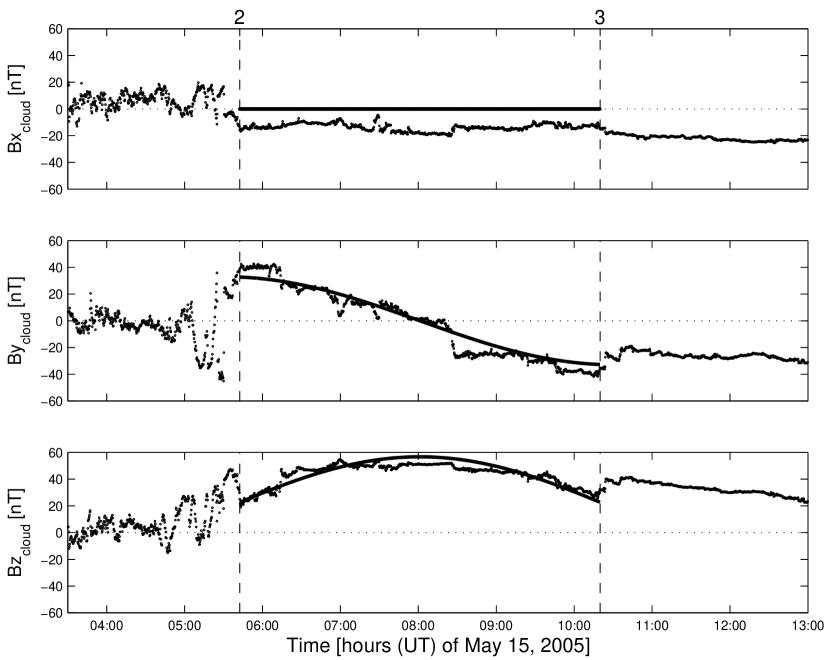
We apply the normalized MV method to the observations between ’2’ and ’3’. We find a left handed flux rope, oriented such that =-15∘ and =125∘, consistent with the SEN orientation determined in Section 2.1. From this orientation and the mean bulk speed (894 km s-1 for this range), we estimate the cloud size perpendicular to its axis as AU.
In the MC frame (see Figure 2), the magnetic field has the typical shape observed in clouds. The almost constant profile (with a mean value nT), indicates that is not zero. Moreover, a rough estimation of can achieved using the expression found by Gulisano et al. (2007) (), which gives .
The MC borders set as ’2’ and ’3’ are in agreement with the expected conservation of magnetic flux across a plane perpendicular to (Dasso et al., 2006), i.e., similar areas below and above the curve which equals before and after the MC center. These boundaries are also in agreement with the expected MD (current sheets) at the interfaces between two structures with different connectivity (as the boundaries of a flux rope forming a MC).
The MC axis, with , is dominantly pointing towards with a significant contribution toward -. This is consistent with the spacecraft passing through the right (west) leg of the flux rope and, thus, with the MC apex located toward the left of L1 (observed from Earth to the Sun, with north upward). From the sign of the observed , the cloud axis is toward the south of the ecliptic.
Fixing the orientation provided by the MV method, we fit the free parameters of Lundquist’s model (see Section 1 for the meaning of the free parameters) and obtain nT and AU-1. Solid lines in panels and in Figure 2 show the curves obtained from the fitting, which are in a very good agreement with the observations (dots).
To validate our previous results, we perform a simultaneous fitting (SF) of the geometrical and physical free parameters using the same procedure and numerical code as Dasso et al. (2006). We obtain =-12∘, =129∘, AU, , nT, AU-1. The agreement between the results of the SF and those from the MV method followed by the fitting of the physical cloud parameters is well within the precision of the methods (the differences are only in the orientation, 5% in the radius and 3% in ). Due to the radial propagation of the solar wind and due to a possible meridional stratification of the solar wind properties, distortions from a cylindrical cross section are expected (see, e.g., Liu et al., 2006b). From a multispacecraft analysis of the first MC observed by STEREO, an oblated transverse size with the major axis perpendicular to the Sun-Earth direction was found (Liu et al., 2008b). The good match between the observations and the cylindrical model (Figure 2) indicates that this flux rope could have an almost cylindrical configuration (a significant ellipticity would have consequences on the magnetic field profile, see Vandas and Romashets (2003)). Therefore, we conclude that the main characteristics of MC1 are well determined.
2.3 Second Magnetic Cloud
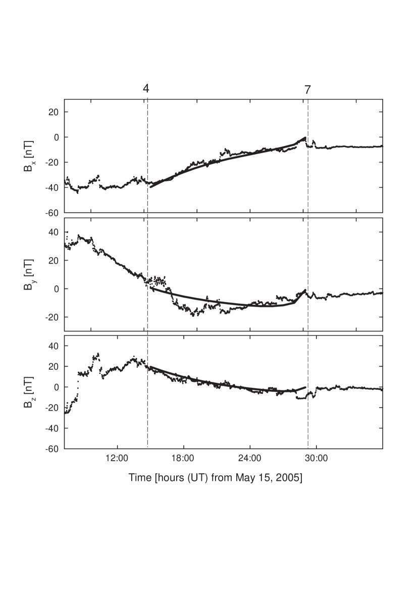
In this section we model the second MC (MC2) observed from ’4’ to ’7’. A decreasing velocity profile (see Section 2.1) indicates that the cloud is in expansion. The sudden change of at ’7’ is the most significant of all changes observed in the field after ’4’; furthermore, after this discontinuity, the expected coherence of is lost. Thus, as previously discussed in Section 2.1, we choose ’7’ as the rear boundary of MC2.
The use of the MV method for this second MC does not provide meaningful results, since the impact parameter is very large as indicated by the low rotation of the magnetic field vector (Figure 1) and also because is the largest field component in the cloud frame [not shown]. Moreover, there is significant expansion, thus normalizing the field is not enough to fully remove this effect. The SF to Lundquist solution, even with a normalized field, cannot provide in this case a reliable result for the same reasons. When the impact parameter is low and the boundaries of the flux rope are well determined, flux rope modelling generally provides a good representation of the magnetic field configuration of a MC (Riley P. et al., 2004). However, models need to be tested using simultaneous observations of different parts of the same flux rope, e.g. as recently done using STEREO observations (Liu et al., 2008b) confirming the flux rope geometry of the studied event. Since simultaneous observations from spacecraft with a significant separation are not available for this event, we apply a different model and method for MC2, described below. This model has more freedom in comparison with Lundquist’s model used before, such as the oblateness of the cloud cross section (Liu et al., 2006b).
Observations of some expanding MCs traveling in the solar wind are consistent with cylindrical expansion (e.g., Nakwacki et al., 2005; Dasso et al., 2007; Nakwacki et al., 2008). However, we can anticipate distortions from the cylindrical shape for MC2 because of the presence of MC1 in its front. Therefore, we compare observations with the model by Hidalgo et al. (2002b), which considers a magnetic field with an elliptical cross section. This model has eight free parameters: the magnetic field strength at the cloud axis, the latitude () and longitude () of the cloud axis, the impact parameter (), the orientation of the elliptical cross section relative to the spacecraft path (), a parameter related to the eccentricity of the cross section (), and two other parameters related to the plasma current density.
3 Solar clues for two source events

3.1 The data
In this section, we analyze solar data from the photosphere to the upper corona in search of two candidate solar events that could be the sources of the two MCs described in previous sections.
The photospheric magnetic field evolution is analyzed using observations from the Michelson Doppler Imager (MDI Scherrer and et al., 1995), on board the Solar and Heliospheric Observatory (SOHO), which measures the line of sight magnetic field at the photosphere. These data are the average of 5 magnetograms with a cadence of 30 seconds. They are constructed once every 96 minutes. The error in the flux densities per pixel in the averaged magnetograms is G, and each pixel has a mean area of Mm2.
At the chromospheric level we have used full-disk H data from Big Bear Solar Observatory (BBSO) and the Optical Solar Patrol Network (OSPAN) at the National Solar Observatory in Sacramento Peak.
To identify changes in the low corona associated to the source regions of the identified MCs, the Extreme-Ultraviolet Imaging Telescope (EIT, Delaboudiniére J.-P. et al., 1995) on board SOHO is used. EIT images chromospheric and coronal material through four filters. In particular, we have analyzed the 195 Å band which images plasma at 1.5106 K. When available we have used observations taken by the Transition Region and Coronal Explorer (TRACE, Handy, 1999) in the 171 Å band.
The identification of CMEs is done using LASCO on board SOHO, plus proxies for eruptions in the chromosphere and lower corona. For the analyzed time interval, LASCO imaged the solar corona from 2 - 30 solar radii with two different coronagraphs: LASCO C2 (2 – 6 solar radii) and C3 (4 – 30 solar radii).
3.2 Solar activity from May 11 to May 12, 2005
Without any doubt, the main contribution to the larger cloud (MC2) and other IP signatures discussed in previous sections is the halo CME appearing in LASCO C2 at 17:22 UT on May 13 (see Sections 3.4 and 3.5). However, since we have found that the ACE magnetic field and plasma observations from 05:42 UT on May 15 (’3’) to 10:30 UT on May 17 (’10’) can be interpreted as being comprised by two different structures (see Sections 2.2- 2.3), we describe the solar activity observed by EIT and LASCO preceding the major CME on May 13.
From May 11 until May 13, 2005, solar activity is mainly concentrated in two ARs, AR 10758 located in the southern hemisphere and AR 10759 in the northern hemisphere, which produces the most intense events. Activity progressively increases in the later region from May 11 to 12; then, flares reach level 2B in H and M1.6 in soft X-rays.
On May 11 a CME is first seen in LASCO C2 at 20:13 UT above the SW limb. This event is classified as a full halo. The linear and second order fittings to LASCO C2 observations give plane-of-sky (POS) speeds of 550 km s-1 and 495 km s-1, respectively (from LASCO CME Catalog, http://cdaw.gsfc.nasa.gov./CME_list/index.html). An M1.1 flare in NOAA AR 10758, located at S11W51, starting at 19:22 UT can be associated with this event. Subframes from the EIT shutterless campaign show a raising feature in absorption by 19:22 UT. However, the closeness in time/space between the two MCs discussed in Section 2.1 makes it highly improbable for this event to be the source of MC1, since by simple assumption of constant speed it would take 3.1 days to reach Earth and then would be expected to arrive before May 15, i.e. earlier than MC1.
On May 12, an event (flare, dimming, and loops in expansion) is seen in EIT at about 1:57 UT. This event originates in AR 10759 and is accompanied with a C9.4 flare located at N11E31 with peak at 1:10 UT. No CME is observed in LASCO. However, a diffuse and gusty outward flow is evident in LASCO C2. There is another apparent event in EIT at about 13:56 UT, to the south of AR 10760. The related C3.0 flare occurs in S11W62 at 13:40 UT. This event shows an association with a CME, weak and slowly traveling in the SW direction. This CME has a strong component in the POS and, therefore, we do not expect it to be significantly directed towards Earth. Furthermore, from the orientation of AR 10760 polarities during their disk transit, we can infer from MDI data that its magnetic helicity sign is positive, contrary to that of both studied MCs (see the description and interpretation of magnetic tongues in López Fuentes et al., 2000, 2003).
After discarding these previous events, and considering the closeness in time/space between the two MCs analyzed in Section 2, we concentrate in the activity observed during May 13. In the next sections we will present observations and discuss, in particular, two flares and associated filament eruptions that we consider to be the solar source events of the clouds. The flare timings are given by GOES soft X-ray data (Figure 4).
3.3 May 13 events: Photospheric and chromospheric signatures
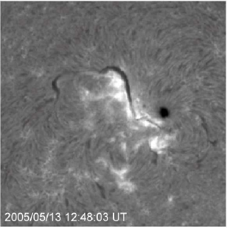
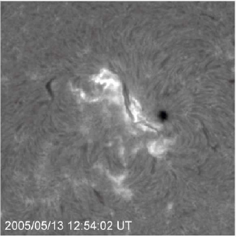
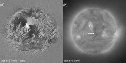
Along May 13 the filament in AR 10759 is seen to activate several times, mainly in its northern fraction. At 12:49 UT a C1.5 flare starts in N17E15, with peak at 13:04 UT. The rising filament is seen in H and also in TRACE (see the left Figure 5 and Section 3.4). At the chromospheric level a two-ribbon flare, classified as a subflare faint, develops along the magnetic inversion line at the north of AR 10759 (Figure 5). This is the only event showing eruptive characteristics at that time on the solar disk. This portion of the inversion line is oriented in the E-W direction. Part of the filament extending along this E-W inversion line is no longer visible by 12:54:02 UT. Flare loops linking the two ribbons are also visible in H at this time. What may be the cause of the destabilization of the E-W portion of the filament? We have analyzed the magnetic changes observed in the filament channel previous to the flare at 12:49 UT, for this we use MDI line of sight magnetic maps. Continuous flux cancellation is observed at the magnetic inversion line along which the erupting part of the filament lies. The E-W northern fraction of the filament shows a non-uniform shape (as being formed by several sections) and some barbs or feet are present (Figure 6 left). A small positive polarity is seen to intrude in the negative field in between two sections of the filament (see the arrow in Figure 6 center); this single intrusion implies a cancellation of Mx. The close relationship between the flare and the magnetic cancellation site is shown in the right panel of Figure 6. MDI low temporal and spatial resolution does not allow us to follow in detail the evolution of the small flux concentrations and ascertain the clear association between their cancellation and filament eruption; however, we believe this to be the most plausible cause. Small-scale magnetic changes in flux concentrations along filament channels have been frequently reported a few hours prior to local filament restructuring (see e.g., Chae et al., 2000; Deng et al., 2002; Wood and Martens, 2003; Schmieder et al., 2006). Furthermore, Zhang et al. (2001) attributed the origin of the major solar flare and filament eruption on July 14, 2000, to flux cancellation at many sites in the vicinity of the active region filament.
Taking into account that the C1.5 flare occurs by only about 4 hours earlier than the main flare and eruption in AR 10759 (see below) and the similar orientation of the MC1 axis and of the magnetic inversion line along which the erupting filament lies (Figure 6 left), we consider that the partial eruption of the AR filament is the source of this first cloud. There is evidence for the breakup of filaments into more than one segment, (see e.g. Martin and Ramsey, 1972) and a recent example in Maltagliati et al. (2006). Even some filaments erupt only partially, or saying it in a different way different portions of the same filament may erupt at different times and trigger different flares (Martin and Ramsey, 1972; Tang, 1986; Maltagliati et al., 2006; Gibson et al., 2006a; Gibson and Fan, 2006; Liu et al., 2008a). This kind of eruptions have been discussed in the frame of the eruptive flux rope model for CMEs (see the review by Gibson et al., 2006b). Moreover, as discussed below in Section 3.5, on May 13 there are no other evidences of CMEs in LASCO until 17:22 UT.
The solar event following the one just described is the major M8.0/2B flare that starts at 16:13 UT and peaks at 16:57 UT. This flare ended on May 14 at 17:00 UT, being a long duration event (see Figure 4). The photospheric and chromospheric observations corresponding to this event have been shown and discussed by Yurchyshyn et al. (2006) and Liu et al. (2007). The former authors have associated this flare and eruption to a single MC comprising the two we have identified in this paper. We want to stress here that the direction of MC2 axis is in agreement with the orientation of the N-S fraction of the AR filament that lies along the main magnetic inversion line (see Figure 6, left panel).
3.4 May 13 events: The lower corona signatures
In the lower corona, TRACE observes the event at 12:49 UT in 171 Å (Figure 7). Images before 12:39:49 UT and after 13:04:27 UT are not useful because of a strong particle shower. TRACE data are dominated by a large-scale sigmoidal structure (with an inverse S shape) previous to the flare well visible by 12:40 UT. The small scale loops linking the two H ribbons are not distinguishable in TRACE images. By 12:49:43 UT the filament can be observed as a dark curved structure surrounded by a brighter one, probably formed by heated filament material (see Figure 7). This bright structure is seen expanding upward until 13:04:27 UT, though it is hard to assure that it erupts because of lack of visibility in the following images (Figure 7, central panels).
Later on, by 16:00 UT (last panel in Figure 7) and before the M8.0 flare, TRACE images appear again dominated by the large-scale sigmoid. This structure is similar to the one described by Liu et al. (2007) seen before the M8.0 flare; in their Figure 1 they show the different parts that constitute the sigmoid: the magnetic elbows, the envelope loops (according to the nomenclature of Moore et al., 2001) and the footpoints of the sigmoidal fields. Thus, the rising of the bright curved structure, shown in the central panels of Figure 7, is most likely linked to the filament eruption during the first and less intense two-ribbon flare that we associate with MC1. Yurchyshyn et al. (2006) have suggested that the bright structure seen in the central panels is the core of the sigmoid that later starts a slow ascent (by 12:55 UT) and become active during the M8.0 flare, but in fact it erupted earlier and reactivated later.
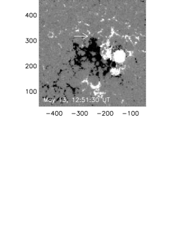
The major eruptive event, linked to an M8.0 flare, is visible in EIT images starting from 16:37 UT (see Figure 8). It exhibits several CME-associated phenomena (Hudson and Cliver, 2001): coronal dimmings, a large-scale EIT wave and a post-eruption arcade. As it was pointed out by Liu et al. (2007), the darkest part of the dimming comprises two patches to the NE and SW of the erupting active region. The SW dimming is associated with a transient coronal hole (shown by an arrow in Figure 8b). It was suggested that transient coronal holes can be interpreted as footpoints of the ejected flux rope (see, e.g., Webb et al., 2000; Mandrini et al., 2005). The absence of the clearly visible second transient coronal hole in this event may indicate that the second leg of the erupted flux rope may have already reconnected with the ambient coronal magnetic field (this reconnection changes the very extended field lines rooted in the dimming by closed magnetic connections Attrill et al., 2006; Kahler and Hudson, 2001). The overall morphology of twin dimmings and the presence of the post-eruption arcade (Figure 8b) suggest that an eruption of a coronal magnetic flux rope had taken place (e.g., Hudson and Cliver, 2001).
3.5 May 13 events: The upper corona observations
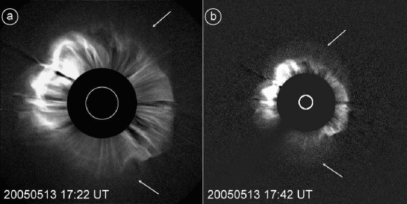
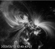
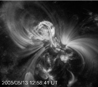
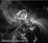
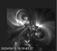
On May 13, 2005, a full halo CME with brightness asymmetry towards the NE first appears in the field of view of LASCO C2 at 17:22 UT (see Figure 9a). Five more partial snapshots of the halo CME were captured by LASCO C3 from 17:20 to 17:50 UT. The closeness in time of the latter images does not allow to see major changes from one to another, so we present here only one of them (Figure 9b). The estimated POS speed for the fastest front, as calculated by the LASCO CME catalog, is 1690 km s-1. Further information on the kinematics of this CME and its associated shock can be found in Section 4 and in Reiner et al. (2007).
Enhancement of the LASCO images presented in Figure 9 allows to distinguish a very faint edge toward the south and north, about a couple of solar radii ahead of the brightest one (indicated by arrows). This feature suggests the presence of a shock, as described by Vourlidas et al. (2003) and Vourlidas (2006). Finally, the CME related to the solar eruption at 12:49 UT is probably so faint, that its detection was not likely due to sensitivity limitations of LASCO (e.g., Tripathi et al., 2004; Yashiro et al., 2005). Furthermore, Yashiro et al. (2005) conclude that all fast and wide CMEs are detectable by LASCO, but slow and narrow CMEs may not be visible when they originate from disk center. In addition to this restriction, which impedes the visualization of a CME if it is feeble, the LASCO cadence during and after the C1.5 flare at 12:49 UT was of 30 minutes, as opposite to the usual 12 minutes of LASCO C2.
4 Two structures in the inner heliosphere: Remote radio type II observations
When a halo CME leaves the field of view of a coronagraph, it is occasionally possible to further track its evolution by means of measurements in the radio regime of the electromagnetic spectrum. The shock commonly driven by a CME excites electromagnetic waves emitted at the local plasma frequency () and/or its harmonic. As the shock travels outward from the solar corona, the local plasma frequency decreases, and a drifting signal, a type II radio burst, is generated. This brand of emissions can be followed drifting in frequency from MHz down to kHz, which is the approximate value of the local plasma frequency in the vicinity of Earth (Leblanc et al., 1998). Then, the shock traveling toward Earth is detected by instruments in the IP space, such as WAVES on board Wind (Bougeret J. L. et al., 1995). The ICME can also be detected by ground-based antennas measuring interplanetary scintillation of radio sources (e.g., Manoharan, 2006).
The metric components of type II bursts have long been used by space weather forecasters as input to models of shock arrival time prediction (e.g., Dryer and Smart, 1984; Smith and Dryer, 1995; Fry et al., 2001). Nevertheless, there is ongoing debate on the mechanism that generates them, questioning their direct relationship with shocks ahead of CMEs (e.g., Pick, 1999; Gopalswamy et al., 2001a; Claßen and Aurass, 2002; Cane and Erickson, 2005). Therefore, Cremades et al. (2007) attempted to improve space weather forecasts by employing information of type II radio bursts in the kilometric domain ( kHz), which are indeed believed to be generated by IP shocks (Cane et al., 1987). Accordingly, the slope of the drifting radio emission can be taken as a proxy for the associated shock speed (Reiner et al., 1998). Furthermore, for each point of emission detected in the space-borne radio receivers, it is possible to obtain a proxy of the radial distance from the Sun through density models (e.g., Saito et al., 1977; Leblanc et al., 1998; Hoang et al., 2007). The technique used to characterize the temporally-associated radio signals makes use of the density model developed by Leblanc et al. (1998). To obtain the approximate sites of the emissions, and consequently a proxy of the shock speed, it is only needed to enter into the density model an estimate of the plasma density near Earth, usually between 5 and 9 cm-3. The top frequency taken into account as input for the technique (300 kHz for the fundamental emission) corresponds approximately to a distance of 20 solar radii according to that heliospheric density model.
We assume that at those heights most of the deceleration has already taken place, and thus that the slope of the linear profile in Figure 10 is enough to characterize the kinematics of a shock that travels at a constant speed. Beyond 20 solar radii, the corresponding frequency channels of the WAVES/RAD1 detector are scarce in comparison with those of WAVES/TNR (see rationale at the end of this Section). That is why the main goal of the latter detector is the tracking of radio phenomena up to the orbit of Earth. Further details on the technique, its application and success relative to other methods can be found in Cremades et al. (2007).
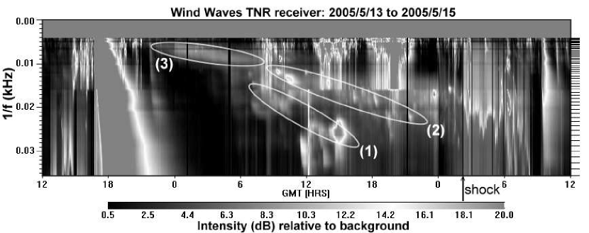
After the solar events on May 13, a number of type II radio features in the kilometric domain were observed by the Thermal Noise Receiver (TNR) experiment on WAVES. Figure 10 displays the radio intensity between May 13 at 12:00 UT and May 15 at 12:00 UT, and from 250 kHz to =20 kHz. In addition, each of the identified low-frequency type II emissions has been labeled as follows: (1) a radio emission drifting at a speed of 1400 km s-1, (2) an emission drifting at a speed of 1450 km s-1 and certainly being the harmonic of the first feature, and (3) a slower radio emission drifting at a speed of 850 km s-1. The application of the technique described in Cremades et al. (2007) to emission (1) yielded for its associated shock a predicted arrival time at 02:40 UT on May 15, which is in good agreement with the real shock arrival at Earth (02:11 UT). The arrival time derived from radio signal (2) yielded 23:20 UT on May 14. The error of 3 hours might be attributed to the ’patchiness’ of the emission. This effect arises because a single shock may drive type II bursts at multiple places along the shock surface, with the possibility of a large non-radial component of the shock velocity. In addition, there could be significant differences in the drift rates if the density gradient or the local shock speed varies along the shock surface. Under these circumstances entities (1, 2) and (3) could be the manifestation of the shock driven by only one ICME. However, we have no data to justify any of these hypothesis. Moreover, the large difference in propagation speed between entities (1, 2) and (3) suggests that they must be indeed produced by two distinct structures traveling in the solar wind or by the same structure traveling with a significantly slower speed at a first stage of its journey and with a faster speed at its second stage. We will interpret this second possibility in the frame of the global observations in next section (Section 5). Finally, the prediction of the arrival time of entity (3) yielded 10:20 UT on May 15. The linear backtracing of this last emission in time matches well with the earlier solar event on May 13. On the other hand, entities (1) and (2) show good temporal association with the occurrence of the second solar event on May 13 (at 16:57 UT).
Based on the observations of WAVES/TNR we present here a different interpretation of the sources of the radio signatures than Reiner et al. (2007), who used radio data acquired by the WAVES/RAD1 detector (see next paragraph). The TNR observations indicate the existence of 2 interplanetary shock entities, which from now on will be referred to as entity (a) -the shock traveling at 1400 km s-1, corresponding to (1) and (2)- and entity (b) -the shock traveling at 850 km s-1, related to (3). Entity (b) presumably draws near entity (a) around 07:00 UT on May 14, at an approximate distance of 98 solar radii from the Sun. There are no visible signs of ’cannibalism’ (Gopalswamy et al., 2001b) in radio data, likely due to the weakness of entity (b) and/or because there is no significant reconnection between the two entities. Moreover, it is worth to note that entity (a) was not visible before 06:00 UT on May 14, as opposite to the slower entity (b). A plausible reason for this effect is that entity (a) may have been moving in an environment plasma faster than the typical solar wind, therefore without leading shock formation.
The kinematics analysis performed for the radio event on May 13-15, 2005 by Reiner et al. (2007) takes into account entity (a) only. Those authors present spectral plots of the event that reach down in frequency up to the coverage of the WAVES/RAD1 detector. As seen in Figure 10 of that study, entity (b) is not obvious from RAD1 measurements. However, it does show up in TNR data, suggesting that Reiner et al. (2007) did not consider those data in their analysis. It is most likely that the poor frequency resolution of RAD1 below 256 kHz is guilty of overseeing entity (b). The RAD1 detector employs at a time only 32 frequency channels to monitor the range 20-1040 kHz, using only 21 channels below 256 kHz and interpolating to obtain the rest of the data. This may lead to false apparent broadband emissions and to the oversight of some narrow-band features in the RAD1 domain. Conversely, the TNR receiver employs 96 channels to cover the frequency range of 4-256 kHz, over five logarithmically spaced frequency bands (Bougeret J. L. et al., 1995, also see location of frequency channels as tick marks on the right vertical axis of Figure 10). This configuration achieves better frequency resolution at distances greater than 20 solar radii, and hence makes it best suitable to study emissions beyond those distances.
5 Conclusion
We propose here a fully consistent physical scenario for the chain of events from May 13 to 17, 2005, which is based on a detailed analysis of the observations presented in previous sections.
Two solar events occurred on May 13 with a difference of 4 hours, both from AR 10759. The first one, a C1.5 two-ribbon flare that was associated with the ejection of a part of the AR filament extending along the E-W portion of the inversion line (north of the AR). The second and largest one, an M8.0 two-ribbon associated with the ejection of the filament lying along the N-S portion of the inversion line and a CME observed in LASCO C2.
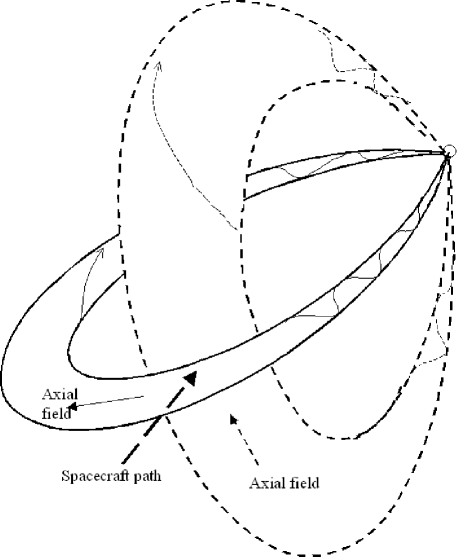
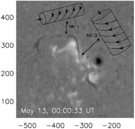
In the IP medium we identify an anomalously long ICME (more than 2 days). Following the results of Burlaga et al. (2001, 2003), this suggest the presence of two flux ropes (see Sect. 2.1). Indeed, we have found two clouds (MC1 and MC2). They are stacked together and only the latitude, , of the magnetic field permits to identify in the data two coherent structures separated by a region (called ’3-4’ in Fig. 1) that have a different temporal evolution from neighboring regions. Such conclusion is supported by the various attempts done to fit the data by one or two flux ropes. Indeed, only the two flux rope models presented in Section 2 give a reasonably good fit to the data. Figure 11 shows a sketch of the two clouds near Earth, in which we have taken into account their orientations, relative sizes, and the spacecraft trajectory during the observations. The two MCs are oriented such that: , , , and . MC1 presents a low impact parameter () and a radius of AU, while MC2 is much larger and presents a larger impact parameter; both MCs have negative magnetic helicity. MC1 is small, has a very intense magnetic field, the signature of an overtaking flow penetrating deep in the out bound, and almost no portion with low proton temperature (see Figure 1); all these observations can be interpreted as the consequence of a compression by MC2.
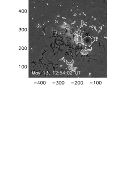
The left panel in Figure 6 shows the projection on the solar surface of the axes of MC1 and MC2 and the sense of their azimuthal field component, for comparison with the orientation of the erupting parts of the filament associated with the C1.5 and M8.0 flares, respectively. Only the second flare has an observed associated CME, and it is apriori surprising to associate a C1.5 flare to a fast ejection (with a velocity km s-1 from radio data); however, it has been shown by Gopalswamy et al. (2003, 2005) that the correlation between CME speed and flare intensity is weak. Apart these two issues, the other characteristics of the solar and interplanetary events are in agreement as follows. The erupting filament orientations and directions of the field in their associated arcades (see right panel of Figure 5 and Figure 8b) are in good agreement with the axial and azimuthal field components in the clouds. The AR field, as well as the two MCs have negative magnetic helicity. Altogether, with the transit time in the expected time interval, this demonstrates the associations between the two solar eruptions to the two interacting MCs detected near Earth.
Moreover, an evidence of the interaction is directly found in the interplanetary radio data, as follow. Radio type II observations (Section 4, entity (b)) are consistent with a speed for the shock driven by the first ejecta (MC1) of km s-1, when it travels from the Sun up to AU (from 13:00 UT on May 13 to 07:00 UT on May 14). The shock driven by the second ejecta (MC2) seems to be weaker and is not detected using radio data in this range of time, probably because MC2 travels in a non-typical solar wind medium, i.e., a medium perturbed by the previous passage of MC1, so having a faster speed. It is also possible that this second shock starts to interact with the trailing part of MC1 at earlier times just after its eruption and, thus, it turns to be weaker, as shown from numerical simulations of interaction of flux ropes (Xiong et al., 2007). Then, at times when MC2 reaches MC1 (at AU, on May 14 at 07:00 UT), when the exchange of momentum between the two clouds is most efficient, MC1 is accelerated and MC2 is decelerated. Then, both start to travel at similar speeds km s-1, but keeping their individuality. The shock wave driven by this new combined structure is the cause of the radio emission observed as entity (a), identified in Section 4. During the second half of the transit to Earth, MC1 is compressed from behind by MC2.
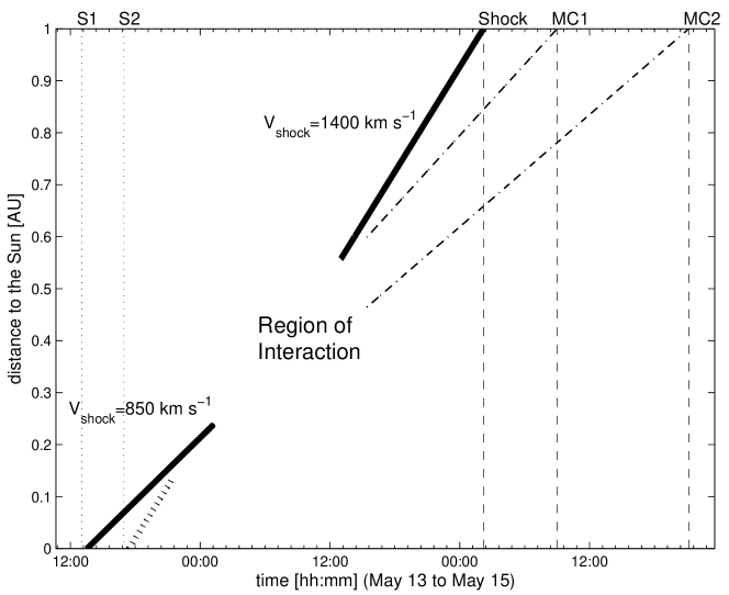
Summarizing, we propose the following interpretation of the sequence of events that occurred on May 13, 2005: two ejective solar events occurred, which could be tracked to the Earth environment and were observed as two attached, but non-merged, magnetic clouds. Figure 12 shows the position versus time (along the Sun-Earth line) of both interplanetary events, as inferred from the sequence of the observations used for our analyses from the Sun to 1 AU. The presence of structures preserving multiple flux ropes, as the multiple structure studied here, has been observed in some cases (Wang et al., 2002). Signatures of the interaction between ejecta, similar to those found in this study, have also been identified from observations with the following properties: (i) acceleration of the leading ejecta and deceleration of the trailing one, (ii) compressed field and plasma in the leading ejecta, (iii) weak shock or disappearance of the shock driven by the second ejecta, and (iv) strengthening of the shock driven by the leading one (Farrugia and Berdichevsky, 2004).
This study especially illustrates the need of combining solar, in situ and remote sensing of interplanetary propagation of the ejecta, in order to reveal the physical processes. Previous studies of the same event, but mostly limited to one of these three domains have concluded on the presence of only one ejecta (with varying characteristics depending on the study). In the present case, the peculiar characteristics of the in situ observed magnetic field first alert us on the possible presence of two MCs. We confirm this by performing a detailed modeling of the magnetic field exploring various flux rope boundaries. This stimulates a deeper study of data in the two other domains, with the new perspective of testing two ejecta. The solar data were crucial to first confirm the presence of two eruptions, and to define the timing and the spatial organization of the erupting magnetic configurations. This brought us to carry a deeper analysis of interplanetary radio observations. Indeed, two type II bursts, traveling at different velocities, were found. These observations also permit to localize where the interaction occurred (about half way between the Sun and the Earth). Then, all the pieces of the puzzle finally fit together, re-enforcing our interpretation separately in each domain. However, the possibility of a single complex event (as proposed by (Yurchyshyn et al., 2006; Reiner et al., 2007)) cannot be fully discarded and our proposed scenario, based on compelling evidence, must be further investigated.
Such studies of interacting ejecta will greatly benefit from observations taken with spacecraft in quadrature, as already done for some events (e.g., Rust et al., 2005), and as available with STEREO spacecrafts. This has already be done with a spacecraft configuration far from optimum conditions (Harrison R. A. et al., 2008). On top of providing in situ measurements of physical parameters at three locations (combining ACE with STEREO) and monitoring type II bursts, there are imminent new possibilities of imaging ICMEs in their journey through interplanetary space. Then, we will have the opportunity to derive precise constraints on the physical mechanisms of interaction of an ejecta with a faster one, or simply with a fast overtaking solar wind.
Acknowledgements.
The authors would like to thank to the International Space Science Institute (ISSI, Bern, Switzerland) for supporting the project ’The Stages of Sun-Earth Connection’, lead by C. Cid. C.C, Y.C, and E.S. acknowledge financial support from the Comisión Interministerial de Ciencia y Tecnolog a(CICYT) of Spain (ESP 2005-07290-C02-01 and ESP 2006-08459). S.D. thanks the Argentinean grant UBACyT X425. S.D. and C.H.M. thank the Argentinean grants: UBACyT X329 and PICT 03-33370 (ANPCyT). H.C., S.D., and C.H.M. are members of the Carrera del Investigador Científico, CONICET. B.S., P.D., and S.P. are doing partly this project in the frame of the European Network “SOLAIRE”. C.H.M., B.S. and P.D. acknowledge financial support from CNRS (France) and CONICET (Argentina) through their cooperative science program (No 20326). L.R. and A.N.Z. acknowledge support from the Belgian Federal Science Policy Office through the ESA-PRODEX programme. The work at the University of Barcelona was supported by the Ministerio de Educación y Ciencia under the projects AYA2004-0322 and AYA2007-60724. We are grateful to the ACE/SWEPAM and ACE/MAG teams, for the data used for this work. We would also like to thank OmniWeb from where we downloaded the preliminar Dst index. The CME catalog is generated and maintained at the CDAW Data Center by NASA and The Catholic University of America in cooperation with the Naval Research Laboratory. We acknowledge the use of Wind WAVES/TNR radio data. The Optical Solar PAtrol Network (OSPAN) project, previously called ISOON, is a collaboration between the Air Force Research Laboratory Space Vehicles Directorate and the National Solar Observatory. We acknowledge the use of TRACE data. EIT, LASCO and MDI data are a courtesy of SOHO/EIT, SOHO/LASCO and SOHO/MDI consortia. SOHO is a project of international cooperation between ESA and NASA. The authors thank S. Hoang for providing clear informations on Wind/WAVES and the referees for their helpful suggestions.References
- Attrill et al. (2006) Attrill, G., M. S. Nakwacki, L. K. Harra, L. van Driel-Gesztelyi, C. H. Mandrini, S. Dasso, and J. Wang, Using the Evolution of Coronal Dimming Regions to Probe the Global Magnetic Field Topology, Sol. Phys., 238, 117–139, 10.1007/s11207-006-0167-5, 2006.
- Bothmer and Schwenn (1994) Bothmer, V., and R. Schwenn, Eruptive prominences as sources of magnetic clouds in the solar wind, Space Sci. Rev., 70, 215–220, 1994.
- Bothmer and Schwenn (1998) Bothmer, V., and R. Schwenn, The structure and origin of magnetic clouds in the solar wind, Annales Geophysicae, 16, 1–24, 1998.
- Bougeret J. L. et al. (1995) Bougeret J. L. et al., Waves: The Radio and Plasma Wave Investigation on the Wind Spacecraft, Space Sci. Rev., 71, 231–263, 10.1007/BF00751331, 1995.
- Brueckner G. E. et al. (1995) Brueckner G. E. et al., The Large Angle Spectroscopic Coronagraph (LASCO), Sol. Phys., 162, 357–402, 10.1007/BF00733434, 1995.
- Burlaga et al. (1981) Burlaga, L., E. Sittler, F. Mariani, and R. Schwenn, Magnetic loop behind an interplanetary shock - Voyager, Helios, and IMP 8 observations, J. Geophys. Res., 86, 6673–6684, 1981.
- Burlaga et al. (2003) Burlaga, L., D. Berdichevsky, N. Gopalswamy, R. Lepping, and T. Zurbuchen, Merged interaction regions at 1 AU, Journal of Geophysical Research (Space Physics), 108, 1425–+, 10.1029/2003JA010088, 2003.
- Burlaga (1988) Burlaga, L. F., Magnetic clouds and force-free fields with constant alpha, J. Geophys. Res., 93, 7217–7224, 1988.
- Burlaga and Ness (1993) Burlaga, L. F., and N. F. Ness, Large-scale distant heliospheric magnetic field: Voyager 1 and 2 observations from 1986 through 1989, J. Geophys. Res., 98, 17,451–17,460, 10.1029/93JA01475, 1993.
- Burlaga et al. (2001) Burlaga, L. F., R. M. Skoug, C. W. Smith, D. F. Webb, T. H. Zurbuchen, and A. Reinard, Fast ejecta during the ascending phase of solar cycle 23: ACE observations, 1998-1999, J. Geophys. Res., 106, 20,957–20,978, 10.1029/2000JA000214, 2001.
- Cane and Erickson (2005) Cane, H. V., and W. C. Erickson, Solar Type II Radio Bursts and IP Type II Events, Astrophys. J., 623, 1180–1194, 10.1086/428820, 2005.
- Cane et al. (1987) Cane, H. V., N. R. Sheeley, Jr., and R. A. Howard, Energetic interplanetary shocks, radio emission, and coronal mass ejections, J. Geophys. Res., 92, 9869–9874, 1987.
- Chae et al. (2000) Chae, J., C. Denker, T. J. Spirock, H. Wang, and P. R. Goode, High-Resolution H Observations of Proper Motion in NOAA 8668: Evidence for Filament Mass Injection by Chromospheric Reconnection, Sol. Phys., 195, 333–346, 2000.
- Cid et al. (2002) Cid, C., M. A. Hidalgo, T. Nieves-Chinchilla, J. Sequeiros, and A. F. Viñas, Plasma and Magnetic Field Inside Magnetic Clouds: a Global Study, Sol. Phys., 207, 187–198, 2002.
- Claßen and Aurass (2002) Claßen, H. T., and H. Aurass, On the association between type II radio bursts and CMEs, Astron. Astrophys., 384, 1098–1106, 10.1051/0004-6361:20020092, 2002.
- Cremades et al. (2007) Cremades, H., O. C. St. Cyr, and M. L. Kaiser, A tool to improve space weather forecasts: Kilometric radio emissions from Wind/WAVES, Space Weather, 5, 10.1029/2007SW000314, 2007.
- Culhane and Siscoe (2007) Culhane, J. L., and G. L. Siscoe, The Sun Earth Workshop: A Summary of the Outcome, Sol. Phys., 244, 3–12, 10.1007/s11207-007-9037-z, 2007.
- Démoulin et al. (2008) Démoulin, P., M. S. Nakwacki, S. Dasso, and Mandrini, Expected in Situ Velocities from a Hierarchical Model for Expanding Interplanetary Coronal Mass Ejections, Sol. Phys., 250, 347–374, 10.1007/s11207-008-9221-9, 2008.
- Dasso et al. (2002) Dasso, S., D. Gómez, and C. H. Mandrini, Ring current decay rates of magnetic storms: A statistical study from 1957 to 1998, J. Geophys. Res., 107, A01,059, 10.1029/2000JA000430, 2002.
- Dasso et al. (2003) Dasso, S., C. H. Mandrini, P. Démoulin, and C. J. Farrugia, Magnetic helicity analysis of an interplanetary twisted flux tube, J. Geophys. Res., 108(A10), 1362, 10.1029/2003JA009942, 2003.
- Dasso et al. (2005) Dasso, S., C. H. Mandrini, P. Démoulin, M. L. Luoni, and A. M. Gulisano, Large scale MHD properties of interplanetary magnetic clouds, Adv. Space Res., 35, 711–724, 10.1016/j.asr.2005.02.096, 2005.
- Dasso et al. (2006) Dasso, S., C. H. Mandrini, P. Démoulin, and M. L. Luoni, A new model-independent method to compute magnetic helicity in magnetic clouds, Astron. Astrophys., 455, 349–359, 10.1051/0004-6361:20064806, 2006.
- Dasso et al. (2007) Dasso, S., M. Nakwacki, P. Démoulin, and C. H. Mandrini, Progressive transformation of a flux rope to an ICME, Sol. Phys., 244, 115–137, 10.1007/s11207-007-9034-2, 2007.
- Delaboudiniére J.-P. et al. (1995) Delaboudiniére J.-P. et al., EIT: Extreme-Ultraviolet Imaging Telescope for the SOHO Mission, Sol. Phys., 162, 291–312, 1995.
- Démoulin (2008) Démoulin, P., A review of the quantitative links between CMEs and magnetic clouds, Annales Geophysicae, 26, 3113–3125, 2008.
- Deng et al. (2002) Deng, Y., Y. Lin, B. Schmieder, and O. Engvold, Filament activation and magnetic reconnection, Sol. Phys., 209, 153–170, 10.1023/A:1020924406991, 2002.
- Dryer and Smart (1984) Dryer, M., and D. F. Smart, Dynamical models of coronal transients and interplanetary disturbances, Adv. Space Res., 4, 291–301, 10.1016/0273-1177(84)90573-8, 1984.
- Farrugia and Berdichevsky (2004) Farrugia, C., and D. Berdichevsky, Evolutionary signatures in complex ejecta and their driven shocks, Annales Geophysicae, 22, 3679–3698, 2004.
- Farrugia C. J. et al. (1999) Farrugia C. J. et al., A Uniform-Twist Magnetic Flux Rope in the Solar Wind, in AIP Conf. Proc. 471: Solar Wind Nine, American Institute of Physics Conference Series, vol. 471, edited by S. T. Suess, G. A. Gary, and S. F. Nerney, p. 745, 1999.
- Fry et al. (2001) Fry, C. D., W. Sun, C. S. Deehr, M. Dryer, Z. Smith, S.-I. Akasofu, M. Tokumaru, and M. Kojima, Improvements to the HAF solar wind model for space weather predictions, J. Geophys. Res., 106, 20,985–21,002, 10.1029/2000JA000220, 2001.
- Gibson and Fan (2006) Gibson, S. E., and Y. Fan, The Partial Expulsion of a Magnetic Flux Rope, Astrophys. J. Lett., 637, L65–L68, 10.1086/500452, 2006.
- Gibson et al. (2006a) Gibson, S. E., Y. Fan, T. Török, and B. Kliem, The Evolving Sigmoid: Evidence for Magnetic Flux Ropes in the Corona Before, During, and After CMES, Space Science Reviews, 124, 131–144, 10.1007/s11214-006-9101-2, 2006a.
- Gibson et al. (2006b) Gibson, S. E., Y. Fan, T. Török, and B. Kliem, The Evolving Sigmoid: Evidence for Magnetic Flux Ropes in the Corona Before, During, and After CMES, Space Science Reviews, 124, 131–144, 10.1007/s11214-006-9101-2, 2006b.
- Goldstein (1983) Goldstein, H., On the field configuration in magnetic clouds, in Solar Wind Conference, pp. 731.–733, 1983.
- Gopalswamy et al. (2000) Gopalswamy, N., A. Lara, R. P. Lepping, M. L. Kaiser, D. Berdichevsky, and O. C. St. Cyr, Interplanetary Acceleration of Coronal Mass Ejections, Geophys. Res. Lett., 27, 145–148, 2000.
- Gopalswamy et al. (2001a) Gopalswamy, N., A. Lara, M. L. Kaiser, and J.-L. Bougeret, Near-Sun and near-Earth manifestations of solar eruptions, J. Geophys. Res., 106, 25,261–25,278, 10.1029/2000JA004025, 2001a.
- Gopalswamy et al. (2001b) Gopalswamy, N., S. Yashiro, M. L. Kaiser, R. A. Howard, and J.-L. Bougeret, Radio Signatures of Coronal Mass Ejection Interaction: Coronal Mass Ejection Cannibalism?, Astrophys. J. Lett., 548, L91–L94, 10.1086/318939, 2001b.
- Gopalswamy et al. (2003) Gopalswamy, N., S. Yashiro, A. Lara, M. L. Kaiser, B. J. Thompson, P. T. Gallagher, and R. A. Howard, Large solar energetic particle events of cycle 23: A global view, Geophys. Res. Lett., 30(12), 120,000–1, 10.1029/2002GL016435, 2003.
- Gopalswamy et al. (2005) Gopalswamy, N., S. Yashiro, S. Krucker, and R. A. Howard, CME Interaction and the Intensity of Solar Energetic Particle Events, in Coronal and Stellar Mass Ejections, IAU Symposium, vol. 226, edited by K. Dere, J. Wang, and Y. Yan, pp. 367–373, 2005.
- Gulisano et al. (2005) Gulisano, A. M., S. Dasso, C. H. Mandrini, and P. Démoulin, Magnetic clouds: A statistical study of magnetic helicity, J. Atmos. Sol. Terr. Phys., 67, 1761–1766, 10.1016/j.jastp.2005.02.026, 2005.
- Gulisano et al. (2007) Gulisano, A. M., S. Dasso, C. H. Mandrini, and P. Démoulin, Estimation of the bias of the minimum variance technique in the determination of magnetic clouds global magnitudes and orientation, Adv. Space Res., 40, 1881–1890, 2007.
- Handy (1999) Handy, B. N. e., The transition region and coronal explorer, Sol. Phys., 187, 229–260, 1999.
- Harrison R. A. et al. (2008) Harrison R. A. et al., First Imaging of Coronal Mass Ejections in the Heliosphere Viewed from Outside the Sun Earth Line, Sol. Phys., 247, 171–193, 10.1007/s11207-007-9083-6, 2008.
- Hidalgo (2003) Hidalgo, M. A., A study of the expansion and distortion of the cross section of magnetic clouds in the interplanetary medium, J. Geophys. Res., 108(A8), 1320, 10.1029/2002JA009818, 2003.
- Hidalgo et al. (2002a) Hidalgo, M. A., C. Cid, A. F. Vinas, and J. Sequeiros, A non-force-free approach to the topology of magnetic clouds in the solar wind, J. Geophys. Res., 107(A1), 1002, 10.1029/2001JA900100, 2002a.
- Hidalgo et al. (2002b) Hidalgo, M. A., T. Nieves-Chinchilla, and C. Cid, Elliptical cross-section model for the magnetic topology of magnetic clouds, Geophys. Res. Lett., 29, 15–1, 10.1029/2001GL013875, 2002b.
- Hoang et al. (2007) Hoang, S., C. Lacombe, R. J. MacDowall, and G. Thejappa, Radio tracking of the interplanetary coronal mass ejection driven shock crossed by Ulysses on 10 May 2001, J. Geophys. Res., 112(A11), A09,102, 10.1029/2006JA011906, 2007.
- Hu and Sonnerup (2001) Hu, Q., and B. U. Ö. Sonnerup, Reconstruction of magnetic flux ropes in the solar wind, Geophys. Res. Lett., 28, 467–470, 10.1029/2000GL012232, 2001.
- Hu and Sonnerup (2002) Hu, Q., and B. U. Ö. Sonnerup, Reconstruction of magnetic clouds in the solar wind: Orientations and configurations, J. Geophys. Res., 107(A7), 1142, 10.1029/2001JA000293, 2002.
- Hudson and Cliver (2001) Hudson, H. S., and E. W. Cliver, Observing coronal mass ejections without coronagraphs, J. Geophys. Res., 106, 25,199–25,214, 10.1029/2000JA004026, 2001.
- Kahler and Hudson (2001) Kahler, S. W., and H. S. Hudson, Origin and development of transient coronal holes, J. Geophys. Res., 106, 29,239–29,248, 10.1029/2001JA000127, 2001.
- Leblanc et al. (1998) Leblanc, Y., G. A. Dulk, and J.-L. Bougeret, Tracing the Electron Density from the Corona to 1 AU, Sol. Phys., 183, 165–180, 1998.
- Leitner et al. (2007) Leitner, M., C. J. Farrugia, C. Möstl, K. W. Ogilvie, A. B. Galvin, R. Schwenn, and H. K. Biernat, Consequences of the force-free model of magnetic clouds for their heliospheric evolution, J. Geophys. Res., 112(A11), A06,113, 10.1029/2006JA011940, 2007.
- Lepping et al. (1990) Lepping, R. P., L. F. Burlaga, and J. A. Jones, Magnetic field structure of interplanetary magnetic clouds at 1 AU, J. Geophys. Res., 95, 11,957–11,965, 1990.
- Liu et al. (2007) Liu, C., J. Lee, V. Yurchyshyn, N. Deng, K.-s. Cho, M. Karlický, and H. Wang, The Eruption from a Sigmoidal Solar Active Region on 2005 May 13, Astrophys. J., 669, 1372–1381, 10.1086/521644, 2007.
- Liu et al. (2008a) Liu, R., H. R. Gilbert, D. Alexander, and Y. Su, The Effect of Magnetic Reconnection and Writhing in a Partial Filament Eruption, Astrophys. J., 680, 1508–1515, 10.1086/587482, 2008a.
- Liu et al. (2005) Liu, Y., J. D. Richardson, and J. W. Belcher, A statistical study of the properties of interplanetary coronal mass ejections from 0.3 to 5.4 AU, Planetary and Space Science, 53, 3–17, 10.1016/j.pss.2004.09.023, 2005.
- Liu et al. (2006a) Liu, Y., J. D. Richardson, J. W. Belcher, J. C. Kasper, and H. A. Elliott, Thermodynamic structure of collision-dominated expanding plasma: Heating of interplanetary coronal mass ejections, Journal of Geophysical Research (Space Physics), 111, 1102–+, 10.1029/2005JA011329, 2006a.
- Liu et al. (2006b) Liu, Y., J. D. Richardson, J. W. Belcher, C. Wang, Q. Hu, and J. C. Kasper, Constraints on the global structure of magnetic clouds: Transverse size and curvature, J. Geophys. Res., 111, A12S03, 10.1029/2006JA011890, 2006b.
- Liu et al. (2008b) Liu, Y., J. G. Luhmann, K. E. J. Huttunen, R. P. Lin, S. D. Bale, C. T. Russell, and A. B. Galvin, Reconstruction of the 2007 May 22 Magnetic Cloud: How Much Can We Trust the Flux-Rope Geometry of CMEs?, Astrophys. J. Lett., 677, L133–L136, 10.1086/587839, 2008b.
- Longcope et al. (2007) Longcope, D., C. Beveridge, J. Qiu, B. Ravindra, G. Barnes, and S. Dasso, Modeling and Measuring the Flux Reconnected and Ejected by the Two-Ribbon Flare/CME Event on 7 November 2004, Sol. Phys., 244, 45–73, 10.1007/s11207-007-0330-7, 2007.
- Lopez (1987) Lopez, R. E., Solar cycle invariance in solar wind proton temperature relationships, J. Geophys. Res., 92, 11,189–11,194, 1987.
- López Fuentes et al. (2000) López Fuentes, M. C., P. Demoulin, C. H. Mandrini, and L. van Driel-Gesztelyi, The Counterkink Rotation of a Non-Hale Active Region, Astrophys. J., 544, 540–549, 10.1086/317180, 2000.
- López Fuentes et al. (2003) López Fuentes, M. C., P. Démoulin, C. H. Mandrini, A. A. Pevtsov, and L. van Driel-Gesztelyi, Magnetic twist and writhe of active regions. On the origin of deformed flux tubes, Astron. Astrophys., 397, 305–318, 10.1051/0004-6361:20021487, 2003.
- Lundquist (1950) Lundquist, S., Magnetohydrostatic fields, Ark. Fys., 2, 361–365, 1950.
- Luoni et al. (2005) Luoni, M. L., C. H. Mandrini, S. Dasso, L. van Driel-Gesztelyi, and P. Démoulin, Tracing magnetic helicity from the solar corona to the interplanetary space, J. Atmos. Sol. Terr. Phys., 67, 1734–1743, 10.1016/j.jastp.2005.07.003, 2005.
- Lynch et al. (2003) Lynch, B. J., T. H. Zurbuchen, L. A. Fisk, and S. K. Antiochos, Internal structure of magnetic clouds: Plasma and composition, J. Geophys. Res., 108(A6), 1239, 10.1029/2002JA009591, 2003.
- Maltagliati et al. (2006) Maltagliati, L., A. Falchi, and L. Teriaca, Rhessi Images and Spectra of Two Small Flares, Sol. Phys., 235, 125–146, 10.1007/s11207-006-1977-1, 2006.
- Mandrini et al. (2005) Mandrini, C. H., S. Pohjolainen, S. Dasso, L. M. Green, P. Démoulin, L. van Driel-Gesztelyi, C. Copperwheat, and C. Foley, Interplanetary flux rope ejected from an X-ray bright point. The smallest magnetic cloud source-region ever observed, Astron. Astrophys., 434, 725–740, 10.1051/0004-6361:20041079, 2005.
- Manoharan (2006) Manoharan, P. K., Evolution of Coronal Mass Ejections in the Inner Heliosphere: A Study Using White-Light and Scintillation Images, Sol. Phys., 235, 345–368, 10.1007/s11207-006-0100-y, 2006.
- Martin and Ramsey (1972) Martin, S. F., and H. E. Ramsey, Early recognition of major solar flares in Halpha ., in Solar Activity Observations and Predictions, pp. 371–387, 1972.
- Marubashi (1997) Marubashi, K., Interplanetary Magnetic Flux Ropes and Solar Filaments, in Coronal Mass Ejections, Geophysical Monograph 99, pp. 147–156, 1997.
- McComas et al. (1998) McComas, D. J., S. J. Bame, P. Barker, W. C. Feldman, J. L. Phillips, P. Riley, and J. W. Griffee, Solar Wind Electron Proton Alpha Monitor (SWEPAM) for the Advanced Composition Explorer, Space Sci. Rev., 86, 563–612, 10.1023/A:1005040232597, 1998.
- Moore et al. (2001) Moore, R. L., A. C. Sterling, H. S. Hudson, and J. R. Lemen, Onset of the Magnetic Explosion in Solar Flares and Coronal Mass Ejections, Astrophys. J., 552, 833–848, 10.1086/320559, 2001.
- Nakwacki et al. (2005) Nakwacki, M. S., S. Dasso, C. H. Mandrini, and P. Démoulin, Helicity analysis for expanding magnetic clouds: A case study, Proc. Solar Wind 11 - SOHO 16, ESA SP-592, 629–632, 2005.
- Nakwacki et al. (2008) Nakwacki, M. S., S. Dasso, C. H. Mandrini, and P. Démoulin, Analysis of large scale MHD quantities in expanding magnetic clouds, J. Atmos. Sol. Terr. Phys., 70, 1318–1326, 2008.
- Pick (1999) Pick, M., Radio and Coronagraph Observations: Shocks, Coronal Mass Ejections and Particle Acceleration, in Proceedings of the Nobeyama Symposium, held in Kiyosato, Japan, Oct. 27-30, 1998, Eds.: T. S. Bastian, N. Gopalswamy and K. Shibasaki, NRO Report No. 479., p.187-198, edited by T. S. Bastian, N. Gopalswamy, and K. Shibasaki, pp. 187–198, 1999.
- Pizzo (1994) Pizzo, V. J., Global, quasi-steady dynamics of the distant solar wind. 1: Origin of north-south flows in the outer heliosphere, J. Geophys. Res., 99, 4173–4183, 1994.
- Reiner et al. (1998) Reiner, M. J., M. L. Kaiser, J. Fainberg, and R. G. Stone, A new method for studying remote type II radio emissions from coronal mass ejection-driven shocks, J. Geophys. Res., 103, 29,651–29,664, 10.1029/98JA02614, 1998.
- Reiner et al. (2007) Reiner, M. J., M. L. Kaiser, and J.-L. Bougeret, Coronal and Interplanetary Propagation of CME/Shocks from Radio, In Situ and White-Light Observations, Astrophys. J., 663, 1369–1385, 10.1086/518683, 2007.
- Riley P. et al. (2004) Riley P. et al., Fitting flux ropes to a global MHD solution: a comparison of techniques, Journal of Atmospheric and Terrestrial Physics, 66, 1321–1331, 10.1016/j.jastp.2004.03.019, 2004.
- Rodriguez L. et al. (2008) Rodriguez L. et al., Magnetic clouds seen at different locations in the heliosphere, Annales Geophysicae, 26, 213–229, 2008.
- Rust et al. (2005) Rust, D. M., B. J. Anderson, M. D. Andrews, M. H. Acuña, C. T. Russell, P. W. Schuck, and T. Mulligan, Comparison of Interplanetary Disturbances at the NEAR Spacecraft with Coronal Mass Ejections at the Sun, Astrophys. J., 621, 524–536, 10.1086/427401, 2005.
- Ruzmaikin et al. (2003) Ruzmaikin, A., S. Martin, and Q. Hu, Signs of magnetic helicity in interplanetary coronal mass ejections and associated prominences: Case study, J. Geophys. Res., 108(A2), 1096, 10.1029/2002JA009588, 2003.
- Saito et al. (1977) Saito, K., A. I. Poland, and R. H. Munro, A study of the background corona near solar minimum, Sol. Phys., 55, 121–134, 1977.
- Scherrer and et al. (1995) Scherrer, P. H., and et al., The Solar Oscillations Investigation - Michelson Doppler Imager, Sol. Phys., 162, 129–188, 1995.
- Schmieder et al. (2006) Schmieder, B., G. Aulanier, P. Mein, and A. López Ariste, Evolving Photospheric Flux Concentrations and Filament Dynamic Changes, Sol. Phys., 238, 245–259, 10.1007/s11207-006-0252-9, 2006.
- Smith et al. (1998) Smith, C. W., J. L’Heureux, N. F. Ness, M. H. Acuña, L. F. Burlaga, and J. Scheifele, The ACE Magnetic Fields Experiment, Space Sci. Rev., 86, 613–632, 10.1023/A:1005092216668, 1998.
- Smith and Dryer (1995) Smith, Z., and M. Dryer, The Interplanetary Shock Propagation Model: A model for predicting solar-flare-caused geomagnetic sudden impulses based on the 2 1/2 D MHD numerical simulation results from the Interplanetary Global Model (2D IGM), Tech. Memo. ERL/SEL-89, NOAA, Washington, D. C., 1995.
- Sonnerup and Cahill (1967) Sonnerup, B. U., and L. J. Cahill, Magnetosphere structure and attitude from Explorer 12 observations , J. Geophys. Res., 72, 171–183, 1967.
- Tang (1986) Tang, F., The two types of flare-associated filament eruptions, Sol. Phys., 105, 399–412, 1986.
- Tripathi et al. (2004) Tripathi, D., V. Bothmer, and H. Cremades, The basic characteristics of EUV post-eruptive arcades and their role as tracers of coronal mass ejection source regions, Astron. Astrophys., 422, 337–349, 10.1051/0004-6361:20035815, 2004.
- Vandas and Romashets (2002) Vandas, M., and E. P. Romashets, Magnetic field in an elliptic flux rope: a generalization of the Lundquist solution, in ESA SP-506: Solar Variability: From Core to Outer Frontiers, pp. 217–220, 2002.
- Vandas and Romashets (2003) Vandas, M., and E. P. Romashets, Force-free field with constant alpha in an oblate cylinder: A generalization of the Lundquist solution, Astron. Astrophys., 398, 801–807, 2003.
- Vourlidas (2006) Vourlidas, A., Detections of CME-Driven Shocks with LASCO, in SOHO-17. 10 Years of SOHO and Beyond, ESA Special Publication, vol. 617, pp. 23.1–23.4, 2006.
- Vourlidas et al. (2003) Vourlidas, A., S. T. Wu, A. H. Wang, P. Subramanian, and R. A. Howard, Direct Detection of a Coronal Mass Ejection-Associated Shock in Large Angle and Spectrometric Coronagraph Experiment White-Light Images, Astrophys. J., 598, 1392–1402, 10.1086/379098, 2003.
- Wang et al. (2005) Wang, A. H., S. T. Wu, and N. Gopalswamy, Magnetohydrodynamic Analysis of January 20, 2001, CME-CME Interaction Event, Geophysical Monographs 156, AGU, pp. 185–195, 2005.
- Wang et al. (2002) Wang, Y. M., S. Wang, and P. Z. Ye, Multiple magnetic clouds in interplanetary space, Sol. Phys., 211, 333–344, 2002.
- Wang et al. (2003) Wang, Y. M., P. Z. Ye, and S. Wang, Multiple magnetic clouds: Several examples during March-April 2001, Journal of Geophysical Research (Space Physics), 108, 1370–+, 10.1029/2003JA009850, 2003.
- Webb et al. (2000) Webb, D. F., R. P. Lepping, L. F. Burlaga, C. E. DeForest, D. E. Larson, S. F. Martin, S. P. Plunkett, and D. M. Rust, The origin and development of the May 1997 magnetic cloud, J. Geophys. Res., 105, 27,251–27,260, 10.1029/2000JA000021, 2000.
- Wood and Martens (2003) Wood, P., and P. Martens, Measurements of Flux Cancellation During Filament Formation, Sol. Phys., 218, 123–135, 10.1023/B:SOLA.0000013027.52104.c6, 2003.
- Wu et al. (1999) Wu, S. T., W. P. Guo, D. J. Michels, and L. F. Burlaga, MHD description of the dynamical relationships between a flux rope, streamer, coronal mass ejection, and magnetic cloud: An analysis of the January 1997 Sun-Earth connection event, J. Geophys. Res., 104, 14,789–14,802, 10.1029/1999JA900099, 1999.
- Wu et al. (2005) Wu, S. T., T. X. Zhang, M. Dryer, X. S. Feng, and A. Tan, The Role of Magnetic Reconnection in CME Acceleration, Space Science Reviews, 121, 33–47, 10.1007/s11214-006-6159-9, 2005.
- Xie et al. (2006) Xie, H., N. Gopalswamy, P. K. Manoharan, A. Lara, S. Yashiro, and S. Lepri, Long-lived geomagnetic storms and coronal mass ejections, J. Geophys. Res., 111(A10), A01,103, 10.1029/2005JA011287, 2006.
- Xiong et al. (2007) Xiong, M., H. Zheng, S. Wu, and S. Wang, Magnetohydrodynamic simulation of the interaction between two interplanetary magnetic clouds and its consequent geoeffectiveness, J. Geophys. Res., 122, A11,103, 10.1029/2007JA012320, 2007.
- Yashiro et al. (2005) Yashiro, S., N. Gopalswamy, S. Akiyama, G. Michalek, and R. A. Howard, Visibility of coronal mass ejections as a function of flare location and intensity, Journal of Geophysical Research (Space Physics), 110, 12–+, 10.1029/2005JA011151, 2005.
- Yurchyshyn et al. (2005) Yurchyshyn, V., Q. Hu, and V. Abramenko, Structure of magnetic fields in NOAA active regions 0486 and 0501 and in the associated interplanetary ejecta, space Weather, 3, 8, 10.1029/2004SW000124, 2005.
- Yurchyshyn et al. (2006) Yurchyshyn, V., C. Liu, V. Abramenko, and J. Krall, The May 13, 2005 Eruption: Observations, Data Analysis and Interpretation, Sol. Phys., 239, 317–335, 10.1007/s11207-006-0177-3, 2006.
- Yurchyshyn et al. (2001) Yurchyshyn, V. B., H. Wang, P. R. Goode, and Y. Deng, Orientation of the Magnetic Fields in Interplanetary Flux Ropes and Solar Filaments, Astrophys. J., 563, 381–388, 2001.
- Zhang et al. (2001) Zhang, J., J. Wang, Y. Deng, and D. Wu, Magnetic Flux Cancellation Associated with the Major Solar Event on 2000 July 14, Astrophys. J. Lett., 548, L99–L102, 10.1086/318934, 2001.