Decoding mode-mixing in black-hole merger ringdown

Abstract

Optimal extraction of information from gravitational-wave observations of binary black-hole coalescences requires detailed knowledge of the waveforms. Current approaches for representing waveform information are based on spin-weighted spherical harmonic decomposition. Higher-order harmonic modes carrying a few percent of the total power output near merger can supply information critical to determining intrinsic and extrinsic parameters of the binary. One obstacle to constructing a full multi-mode template of merger waveforms is the apparently complicated behavior of some of these modes; instead of settling down to a simple quasinormal frequency with decaying amplitude, some $|m|\neq\ell$ modes show periodic bumps characteristic of mode-mixing. We analyze the strongest of these modes – the anomalous $(3,2)$ harmonic mode – measured in a set of binary black-hole merger waveform simulations, and show that to leading order, they are due to a mismatch between the spherical harmonic basis used for extraction in 3D numerical relativity simulations, and the spheroidal harmonics adapted to the perturbation theory of Kerr black holes. Other causes of mode-mixing arising from gauge ambiguities and physical properties of the quasinormal ringdown modes are also considered and found to be small for the waveforms studied here.

I Introduction

Since the first successful simulation of black-hole binaries (BHBs) through late inspiral, merger, and ringdown in 2005 Pretorius (2005); Campanelli et al. (2006a); Baker et al. (2006a), theoretical interest has centered on the resulting gravitational waveforms. A crucial tool in waveform studies has been the analysis of the radiation wave pattern in spherical harmonic components. This decomposition is useful both in the physical interpretation of the radiation, and in structuring the waveform information content for the development of approximate analytic or empirical encodings.

The self-consistency of results for the dominant quadrupole waveforms across numerical codes was quickly established Baker et al. (2007); Hannam et al. (2009), enabling rapid study of the basic characteristics of mergers Campanelli et al. (2006b); Buonanno et al. (2007); Boyle et al. (2007); Scheel et al. (2009); González et al. (2009); Lousto et al. (2010a); Centrella et al. (2010); Hinder (2010) Researchers soon began to build analytic template models compatible with these numerical results as well as with the post-Newtonian (PN) at earlier times, to provide relatively quick waveforms for specified BHB source masses and spins Ajith et al. (2011); Pan et al. (2010); Santamaría et al. (2010). While expected to be sufficient for detection of BHB mergers, quadrupole-only templates will not lock down most of the intrinsic (masses, spin magnitudes & directions) and extrinsic (sky position, phase) BHB system parameters. To gain an understanding of these parameters requires a richer template bank, one that includes all of the relevant angular modes of the signal Arun et al. (2007a, b); Trias and Sintes (2008); McWilliams et al. (2010).

Working with a spherical harmonic basis of spin-weight $s=-2$ Goldberg et al. (1967); Wiaux et al. (2007), several studies Berti et al. (2007, 2008); Baker et al. (2008); Kelly et al. (2011); Pan et al. (2011) have found that after the dominant quadrupole $(\ell=2,m=\pm 2)$ modes, the next most important modes tend to be the higher $m=\pm\ell$ modes: $(3,\pm 3)$, $(4,\pm 4)$, etc., though odd-$m$ modes are sometimes suppressed by symmetry. We have also seen, however, that certain $m<|\ell|$ modes can be important. Prominent amongst these are the $(2,\pm 1)$ and $(3,\pm 2)$ modes. Figure 1 shows the radiative power for the most important modes in the case of the merger of a 4:1 nonspinning BHB. Here we see that the $(2,1)$ mode has actually overtaken the $(5,5)$ mode in importance by merger time.

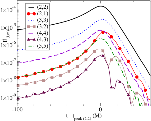
Figure 1: Gravitational-wave luminosity from the merger and ringdown of a nonspinning black-hole binary of mass ratio 4:1, decomposed by harmonic mode.

A key feature of BHB mergers exposed through the spherical harmonic decomposition waveform studies is the rather clean separation of the sometimes complicated mix of signal frequencies, achieved by angular-mode decomposition. Even when typical observers would measure complicated wave shapes combining several frequency harmonics, these harmonics largely reduce to slowly evolving sinusoids in each spherical harmonic component mode. To a very good approximation, this structure holds consistently through the inspiral, merger, and ringdown Baker et al. (2002a, b); Berti et al. (2007); Baker et al. (2006b). This pattern of frequency separation is extremely convenient in allowing relatively simple encodings of the waveform information in analytic models.

Partly because of these properties, angular-mode decomposition has become a standard approach to comparing waveform simulations with each other, with analytic post-Newtonian calculations, and with developing empirical waveform template models. These uses of the decomposition technique have elevated its significance from its beginning as an interpretive convenience to its current status as an essential component of how we quantitatively understand gravitational-wave signals. Thus we must be aware of the possibility that artifacts of arbitrary choices in the details of the decomposition procedure may interfere with our quantitative understanding of the waveforms themselves.

Such concerns are particularly notable when we see unusual features in the decomposed waveforms seeming to violate the a posteriori expectation of clean separation of frequencies. Several authors Buonanno et al. (2007); Schnittman et al. (2008); Baker et al. (2008); Pan et al. (2011); Kelly et al. (2011) have noted that the $(3,2)$ mode in particular typically seems to break from this simple pattern, showing unusual post-merger features that require investigation and resolution before a useful model can be developed. In some of the earliest merger simulations, Buonanno et al. Buonanno et al. (2007) already noted the presence in the post-merger “ringdown” $(3,2)$ mode of both $(3,2)$ and $(2,2)$ quasinormal-mode (QNM) frequencies.

Existing multiple-mode template banks for low-eccentricity coalescences generally assume a monotonic increase in frequency, and a simple single-peaked corresponding amplitude for each mode. Although the $(3,2)$ mode is generically much weaker than the first few $\ell=m$ modes, if such template models are applied to it naïvely, they may suffer significant biases in their fitting parameters. How serious the effect might be on parameter-estimation studies using these template banks is unknown at the time of writing.

In this paper, we investigate these $(3,2)$-mode anomalies, with a survey of 3D numerical simulations of the merger of various comparable-mass BHBs with non-precessing spins, exploring a range of possible “causes”. We find that the dominant part of the measured mode-mixing that underlies the anomalous effect can be attributed to our use of spherical harmonics rather than the spheroidal harmonics expected by Teukolsky perturbation theory.

The remainder of this paper is laid out as follows: In Sec. II, we review the numerical evidence for mode-mixing in existing $(3,2)$ evolutions, and show how well it is captured by a simple two-mode phenomenological model for the ringdown waveform segment. In Sec. III, we discuss general models for why mode-mixing should be expected, including effects of coordinate distortions in the radiation extraction spheres, and of ill-adapted harmonic basis functions in the radiation decomposition. In Sec. IV, we introduce our set of expanded numerical evolutions, arranged into “equivalence classes” of common end-state Kerr spins, which we analyze in Sec. V, fitting the measured contributions of two-mode models to our models. We conclude in Sec. VI with discussion on the application of these results to more general late-merger-ringdown models, such as the implicit rotating source model of Refs. Baker et al. (2008); Kelly et al. (2011). We present a detailed description of our selection of equivalence classes of binaries in Appendix B.

II Bumps in Numerical $(3,2)$ Modes

The first gravitational waveforms extracted from numerical simulations were the dominant $(2,\pm 2)$ modes, whose early-inspiral behavior was expected to match the quadrupole radiation predicted by quasi-Newtonian and post-Newtonian theory. Once these had been shown to be robust and universal across codes Baker et al. (2007); Hannam et al. (2009), some groups turned their attention to the subdominant modes. Analyzing the subdominant modes of equal-mass binaries, Buonanno et al. Buonanno et al. (2007) reported that an accurate fit of the $(3,2)$ mode for the ringdown stage of effective-one-body (EOB) waveforms requires the addition of the fundamental $(2,2)$ quasinormal frequency. When Baker et al. Baker et al. (2008) looked at a set of mergers of nonspinning black-hole binaries with mass ratios in the range 1:1 to 6:1, they noted that one of the leading subdominant modes, $(3,2)$, showed an unusual bumpiness just after merger over a range of parameter space. This bumpiness manifested in both the frequency and amplitude, and appeared to persist with both increased resolution and extraction radius, thus constituting a robust pattern of excursions from the frequency separation dominating the $\ell=m$ modes. More recent work by Kelly et al. Kelly et al. (2011) shows the same anomaly in equal-mass binaries with non-precessing spins (i.e., the spins are aligned/anti-aligned with the orbital angular momentum).

Examples of these more complicated waveform features are shown in Fig. 2, where we plot waveform frequency (top panel) and amplitude (bottom panel) of the measured $(3,2)$ mode for the merger of a nonspinning 4:1 binary, as well as for the mergers of several other BH configurations with the same final dimensionless spin ($\alpha_{\rm f}\approx 0.475$). We also mark the expected real QNM $(2,2)$ and $(3,2)$ frequencies, $\omega_{22}$ and $\omega_{32}$ for a Kerr black hole of this spin. From the time of peak amplitude ($t=0$ here) until the waveforms start to degrade around $60M$ later, the frequency seems to oscillate around one or other of these two QNM frequencies, rather than locking onto the higher $\omega_{32}$, as for other modes. These oscillations appear in the strain $h$ and its time-derivatives; we choose to study strain-rate, $\dot{h}(t)$, waveforms, which we decompose into modes $\dot{h}_{(\ell,m)}(t)=|\dot{h}_{(\ell,m)}|\exp(i\varphi_{(\ell,m)})$, with instantaneous frequencies $\dot{\varphi}_{(\ell,m)}$.

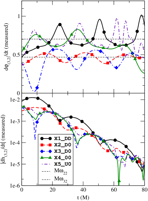
Figure 2: Post-merger frequency [top panel] and amplitude [bottom panel] of the numerically measured $(3,2)$ mode for a set of “4:1-equivalent” evolutions, resulting in a final black hole with dimensionless spin $\alpha_{\rm f}\approx 0.475$, matching that of a 4:1 nonspinning binary merger. The data sets have been shifted in time so that $t=0$ corresponds to peak amplitude of the dominant $(2,2)$ mode. The two dashed (black) horizontal lines in the top panel mark the fundamental QNM frequencies $\omega_{22}$ (lower) and $\omega_{32}$ (higher) for a Kerr hole of the same final spin.

We can model the more complicated ringdown waveform features by expressing the $(2,2)$ mode as a pure QNM ringdown, and the measured $(3,2)$ mode as a linear combination of QNM ringdowns:

$$\dot{h}_{(2,2)}^{\rm model} =A_{22}e^{i(\sigma_{22}t+\delta_{22})},$$ (1)

$$\dot{h}_{(3,2)}^{\rm model} =A_{32}e^{i(\sigma_{32}t+\delta_{32})}+\rho_{32}A_{22}e^{i(\sigma_{22}t+\delta_{22})}.$$ (2)

Here $\sigma_{\ell m}\equiv\omega_{\ell m}+i/\tau_{\ell m}$ is the full complex QNM frequency, and $\rho_{32}\equiv\rho_{0}\exp(i\zeta)$ is a constant complex-valued parameter indicating the mixing of the $(2,2)$ QNM mode into the measured $(3,2)$ mode. The modeled $(3,2)$ mode frequency and amplitude are then:

$$\dot{\varphi}_{(3,2)}^{\rm model}(t)= \omega_{32}+\frac{\varepsilon(t)^{2}\Delta_{R}}{F(t)}$$ (3)

$$-\frac{\varepsilon(t)\left[\Delta_{R}\cos(\Delta_{R}t+\delta)+\Delta_{I}\sin(\Delta_{R}t+\delta)\right]}{F(t)},$$

$$\left|\dot{h}_{(3,2)}^{\rm model}(t)\right|= A_{32}e^{-t/\tau_{32}}\sqrt{F(t)}.$$ (4)

where $F(t)\equiv 1+2\varepsilon(t)\cos(\Delta_{R}t+\delta)+\varepsilon(t)^{2}$, $\Delta_{R}\equiv\omega_{32}-\omega_{22}$, $\Delta_{I}=1/\tau_{32}-1/\tau_{22}$, $\varepsilon(t)\equiv\rho_{0}A_{22}/A_{32}\exp(\Delta_{I}t)\equiv\varepsilon_{0}\exp(\Delta_{I}t)$, and $\delta\equiv\delta_{32}-\delta_{22}-\zeta$.

For a given mass and spin, the QNM frequencies, $\omega_{22}$ and $\omega_{32}$, and the damping times, $\tau_{22}$ and $\tau_{32}$, are values known from black-hole perturbation theory. Typically, $\tau_{22}\approx\tau_{32}$, so that $\Delta_{I}$ is somewhat smaller than $\Delta_{R}$, allowing a beat-like effect to persist over several cycles. Fixing these leaves just two free parameters for the frequency: $\varepsilon_{0}\equiv\rho_{0}A_{22}/A_{32}$, the initial ratio of contributing amplitudes, and $\delta$, the initial phase difference, as well as one more amplitude parameter, $A_{32}$.

Evidently, the characteristic shape of the modeled (3,2) mode frequency plots will depend on the relative magnitude of the modal contributions: for $\varepsilon_{0}\ll 1$, the frequency will oscillate (approximately) sinusoidally about $\omega_{32}$; for $\varepsilon_{0}\gg 1$, the oscillation will be about $\omega_{22}$; for intermediate values, the oscillatory shape will be more complex. In the left panel of Fig. 3, we demonstrate these shapes for a Kerr hole of spin $\alpha_{\rm f}=0.475$, the same 4:1 end-state spin as in Fig. 2. Similarly, the right panel shows the corresponding modal amplitude shape for the same end-state hole. Again, the most extreme bumps in amplitude occur when the $(2,2)$ and $(3,2)$ modes have comparable amplitude contributions ($\varepsilon_{0}\sim 1$). These theoretical curves should be compared with the numerically measured mixing in Fig. 2.

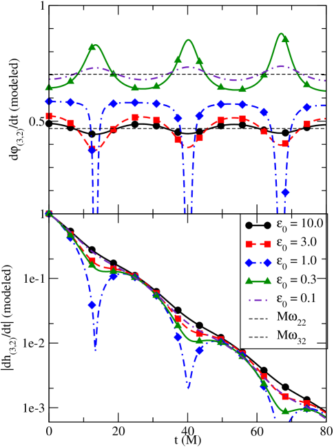
Figure 3: Possible shapes from Eqs. (3)-(4) for the modeled $(3,2)$ mode frequency [top panel] and amplitude [bottom panel] resulting from a merger with an $\alpha_{\rm f}=0.475$ endpoint. All curves assume zero phase difference $\delta$, and overall amplitude is arbitrarily scaled to unity at $t=0$. As with Fig. 2, the two dashed (black) horizontal lines in the top panel mark the fundamental QNM frequencies $\omega_{22}$ (lower) and $\omega_{32}$ (higher) for a Kerr hole of the same final spin.

III Possible Causes of Mode-Mixing

The bumpy features seen in the measured $(3,2)$ mode are a clear exception to the general rule that each angular mode encodes sinusoidal waves with just one slowly evolving frequency component, the phenomenon we refer to as frequency separation. In Fig. 3, we showed that a combination of the fundamental $(3,2)$ and $(2,2)$ quasinormal-mode frequencies produces similar features. More generally, there are indications that such mixing occurs among other modes, especially other higher-order $m=2$ modes, which likewise seem prone to coupling to the dominant mode. Here we ask the basic question: is this mode-mixing a fundamental property of the radiation, or some kind of an artifact, and if so, what kind?

We consider various hypotheses to explain this mode-mixing effect violating our empirical frequency separation rule. The first, which we label physical mixing, is simply that the frequency separation rule does not physically hold to sufficiently high precision; that is we are are perhaps seeing a nonlinear effect in the radiation-generation process underlying the $(3,2)$ mode. Under this assumption, no choice of fixed or slowly evolving angular basis could be expected to yield the kind of frequency separation we see in other cases. Near the merger where nonlinear physics is dominant, it is difficult to make any strong argument for expecting frequency separation. Indeed, we would be surprised to not find violations of this assumption as we probe beyond the first few orders of magnitude in waveform precision.

In the linear ringdown dynamics where this investigation is focused, some degree of physical frequency separation can be expected, based on the separability of the Teukolsky equation, which describes small distortions of a stationary black-hole spacetime. The scale of physical linear mode-mixing can be quantified by careful consideration of quasinormal modes.

The alternative hypothesis is that the mixing is an artifact of our analysis, arising from choices that we make in setting up the angular-mode decomposition. Perhaps our basis is not quite optimal, but we can find some other basis in which we more precisely recover frequency separation. Indeed, given the freedom available in selecting such a representation, we have little grounds for supposing that our first guess would be optimal. Here we consider two classes of choices in how to represent the space of gravitational radiation waveforms, which, in the full sense, has angular and retarded-time dimensions.

The first choice we make is in how we define the spheres on which angular harmonic decomposition will be conducted. Within the structure of asymptotically flat spacetimes, gauge freedom in the choice of constant-retarded-time spheres can yield a frequency-dependent mode-mixing effect in the decomposed waveforms. This ambiguity arises from the freedom to re-parameterize the proper-time coordinate, the so-called “supertranslations” subgroup of the Bondi-Metzner-Sachs gauge group for outgoing radiation. We describe this possibility of supertranslation gauge mixing in more detail below. We may generally expect that mode-mixing of this sort will be most evident in the late merger, where wavelengths are shortest.

The next choice we make is in choosing the family of angular basis functions on the extraction spheres. In this case, the mixing arises if our chosen family of modal basis functions used for radiation extraction differs from the optimal one in which frequency separation is best approximated. It is common to apply a spin-weighted spherical-harmonic basis, but a different choice may be motivated for the ringdown signals. Indeed, the separation of the Teukolsky equation is not achieved in a spin-weighted spherical harmonic basis, but in a spin-weighted spheroidal-harmonic basis. It has been suggested Buonanno et al. (2007); Berti et al. (2007) that this difference explains the sort of waveform phenomena we consider, though this has not been demonstrated. We label this effect angular-basis mixing.

In the next subsections, we consider these possible mixing effects in detail, preparing for a quantitative study of the evidence for these effects in numerical data in Sec. V.

III.1 Gauge Effects

To understand the effect we are calling supertranslation gauge mixing, we must make a brief detour to describe the gauge freedom in the representation of an outgoing radiation field approaching future null infinity in an asymptotically flat spacetime. Consider such a spacetime in standard retarded-time coordinates $\{u,r,\theta,\phi\}$. Scaled by $r$, the outgoing radiation field propagates outward on null rays labeled by $u,\theta$, and $\phi$. Each polarization component can thus be described by a function of these variables. The Bondi-Metzner-Sachs (BMS) Bondi et al. (1962); Sachs (1962) group describes gauge transformations among these variables of the form

$$\theta^{\prime}=\theta^{\prime}(\theta,\phi),\;\;\phi^{\prime}=\phi^{\prime}(\theta,\phi),\;\;u^{\prime}=K(\theta,\phi)\left(u-\alpha(\theta,\phi)\right),$$

where $(\theta,\phi)\rightarrow(\theta^{\prime},\phi^{\prime})$ is a conformal transformation on a constant-$u$ sphere with conformal factor $K$.

For concreteness in the context of numerical relativity simulations, we note that it is common to make these gauge choices by specifying an “extraction sphere” located sufficiently far from the source where radiation field calculations are realized. The effect of one class of BMS transformations, amounting to rotations of the extraction sphere, has been identified as an important concern when the choice of axis is not fixed by symmetry Gualtieri et al. (2008); Campanelli et al. (2009); Schmidt et al. (2011); O’Shaughnessy et al. (2011, 2012); Schmidt et al. (2012). However, the simulations in this study involve nonprecessing mergers, with no ambiguity in defining the orientation of the extraction sphere.

But what happens if we make a small radial perturbation of the extraction sphere? It is clear that sufficiently small distortions of larger extraction spheres would have negligible impact on the intrinsic geometry of the sphere. The gauge effects of such distortions are described by a subset of the BMS transformations, known as supertranslations, with $\theta^{\prime}=\theta,\phi^{\prime}=\phi$, and $K=1$.

Now consider the effect of a supertranslation on a gravitational waveform $\psi(u,\theta,\phi)$. Here we will make the additional assumption that $\alpha(\theta,\phi)$ is sufficiently small that we can approximate the effect of the supertranslation by

$$\psi(u^{\prime},\theta,\phi)\approx\psi(u,\theta,\phi)+\alpha(\theta,\phi)\frac{\partial}{\partial u}\psi(u,\theta,\phi),$$ (5)

and we can expand the supertranslation in terms of (scalar) spherical harmonics:

$$\alpha(\theta,\phi)=\sum_{LM}b_{LM}\,{\,}\,_{0}Y_{L}^{M}(\theta,\phi).$$ (6)

Then from (5), the measured radiation modes will be perturbed as follows:

$$\psi_{\ell m}(u^{\prime})\approx\psi_{\ell m}(u)+\sum_{\ell^{\prime}m^{\prime}}{C_{\ell m\ell^{\prime}m^{\prime}}\frac{\partial}{\partial u}\psi_{\ell^{\prime}m^{\prime}}(u)},$$ (7)

where

$$C_{\ell m\ell^{\prime}m^{\prime}}=\sum_{LM} b_{LM}\oint{\,}\,_{0}Y_{L}^{M}{\,}\,_{-2}Y_{\ell^{\prime}}^{m^{\prime}}{\,}\,_{-2}Y_{\ell}^{m*}{\,}d\Omega$$

$$=\sum_{LM} b_{LM}\left[\frac{\left(2L+1\right)\left(2\ell^{\prime}+1\right)}{4\pi\left(2\ell+1\right)}\right]^{1/2}$$

$$\times\left<L,0,\ell^{\prime},2|\ell,2\right>\left<L,M,\ell^{\prime},m^{\prime}|\ell,m\right>.$$ (8)

In this paper we focus on mixing from the dominant mode, ($\ell^{\prime}=2,m^{\prime}=2$), with another $m=2$ mode, fixing these values. For these cases the Clebsch-Gordan selection rules require that $M=0$ and $\ell-2\leq L\leq\ell+2$. Then our mixing coefficient takes the form

$$C_{\ell 222}=\sum_{L}b_{L0}\left[\frac{5\left(2L+1\right)}{4\pi\left(2\ell+1\right)}\right]^{1/2}\left<L,0,2,2|\ell,2\right>^{2}.$$ (9)

For example, complete expansions for $\ell=3$ and $\ell=4$ would yield

$$C_{3222} =\sqrt{\frac{5}{7\pi}}\frac{1}{132}\left(22\sqrt{3}b_{10}+33\sqrt{5}b_{20}+22\sqrt{7}b_{30}\right.$$

$$\left.+22b_{40}+\sqrt{11}b_{50}\right),$$

$$C_{4222} =\sqrt{\frac{5}{\pi}}\frac{1}{4004}\left(143\sqrt{5}b_{20}+286\sqrt{7}b_{30}+702b_{40}\right.$$

$$\left.+91\sqrt{11}b_{50}+14\sqrt{13}b_{60}\right).$$

The shape of the distorted extraction sphere is determined by the coefficients $b_{L0}$: for real $\alpha$, we need the $b_{L0}$ also to be real. The reality of the Clebsch-Gordan coefficients then implies that $C_{\ell 222}$ is also real.

The other ingredient in the waveform-mode perturbation (7) is the derivative with rrespect to $u$ on the right-hand side:

$$\partial_{u}\psi_{\ell^{\prime}m^{\prime}}(u)=\partial_{u}\left(A(u)e^{i\varphi(u)}\right)=\left(\frac{\dot{A}}{A}+i\dot{\varphi}\right)\psi_{\ell^{\prime}m^{\prime}}(u).$$

After merger, the effective coefficient $\left(\dot{A}/A+i\dot{\varphi}\right)$ will asymptote to a constant complex number:

$$\left(\frac{\dot{A}}{A}+i\dot{\varphi}\right)\rightarrow-\frac{1}{\tau_{\ell^{\prime}m^{\prime}}}+i\omega_{\ell^{\prime}m^{\prime}}=i\sigma_{\ell^{\prime}m^{\prime}}.$$

This implies a simple, QNM-driven leakage from the $(2,2)$ mode into higher-$\ell$ modes. Collecting terms, and working with the strain-rate $\dot{h}$, during ringdown we have

$$\dot{h}_{(\ell,2)}^{\rm gauge} \approx\dot{h}_{(\ell,2)}+iC_{\ell 222}\,\sigma_{22}\,\dot{h}_{(2,2)}$$

$$=\dot{h}_{(\ell,2)}+\rho_{{\rm gauge},\ell 2}\,\dot{h}_{(2,2)}.$$ (10)

In Fig. 4, we show the real and complex parts of the leakage parameters $\rho_{{\rm gauge},32}$ and $\rho_{{\rm gauge},42}$ for the sweep of end-state spins $\alpha_{\rm f}$, assuming an unchanging scaling $b_{20}=1$ (and all other $b_{L0}=0$). The value of $b_{20}$ is not physical, but gauge, and may differ between any two waveform determinations. The most important property we note is that the BMS leakage coefficients are nearly pure-imaginary at any fixed $b_{20}$ and any spin $\alpha_{\rm f}$.

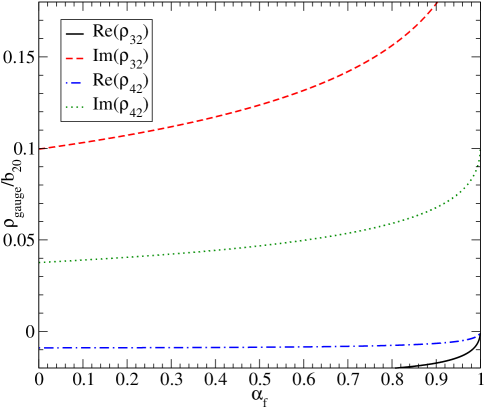
Figure 4: Real and imaginary parts of $\rho_{{\rm gauge},32}$ and $\rho_{{\rm gauge},42}$ (for $b_{20}=1$) for post-merger Kerr BHs of dimensionless spin $\alpha_{\rm f}$ (and corresponding fundamental $(2,2)$ QNM frequency $M_{\rm f}\sigma_{22}$).

III.2 Angular Basis Effects

Another possible path to mixing arises from considering what quasinormal-mode (QNM) frequencies actually represent. QNMs were originally discovered in numerical black hole scattering studies Vishveshwara (1970); Press (1971) and eventually understood as a key feature of the perturbation theory of Kerr black holes Teukolsky (1972). In developing this theory, Teukolsky worked with a background Kerr black hole in a very specific coordinate system due to Boyer & Lindquist Boyer and Lindquist (1967).

A perturbed Kerr black hole will ring down to quiescence through the emission of gravitational waves. These waves will have characteristic frequencies $\omega_{\ell m}$ and damping times $\tau_{\ell m}$ given by the hole’s QNM spectrum. While the primary aim of QNM analysis is to determine the set of allowed complex frequencies $\sigma_{\ell m}\equiv\omega_{\ell m}+i/\tau_{\ell m}$, these frequencies are tied to the radial and angular eigenfunctions arising from the separation of the perturbation equations. These angular eigenfunctions are the spin-weighted spheroidal harmonics, $\,{}_{-2}\mathcal{Y}_{\ell}^{m}(M\alpha\sigma;\theta,\phi)\equiv\,_{-2}S_{\ell}^{m}(M\alpha\sigma;\cos\theta)e^{im\phi}$.

Numerical waveform extraction from binary mergers, on the other hand, typically decomposes the waveforms onto the more generally motivated basis of spin-weighted spherical harmonics $\,{}_{-2}Y_{\ell}^{m}(\theta,\phi)$, which correspond to a spheroidal harmonic basis with $M\alpha\sigma=0$: $\,{}_{-2}Y_{\ell}^{m}(\theta,\phi)\equiv\,_{-2}\mathcal{Y}_{\ell}^{m}(0;\theta,\phi)$ Teukolsky (1972). Buonanno et al. Buonanno et al. (2007) demonstrated that using a spherical harmonic basis will necessarily result in mixing of $(\ell,m)$ and $(\ell^{\prime},m)$ quasinormal modes. Without an obvious nontrivial choice for $M\alpha\sigma$ that applies at all times, for all modes, over the course of the evolving simulation, decomposing with $M\alpha\sigma\rightarrow 0$ seems a natural choice. Here we consider an alternative choice, $M\alpha\sigma\rightarrow M_{\rm f}\alpha_{\rm f}\sigma_{22}$, hoping to limit much of the mode mixing. Using this basis requires knowing the final Kerr state $(M_{\rm f},\alpha_{\rm f})$ of the merger before the decomposition can be applied, and the additional task of numerically computing the basis functions (see Appendix A). Still this basis is not optimal for the subdominant modes. This unavoidable sub-optimality is discussed further in the next subsection. The distinction between the spheroidal and spherical harmonics may be expected to yield the appearance of mode-mixing in the numerical waveform results even if we have eliminated the gauge freedom noted in the last section by optimal correspondence with a suitably perturbed Boyer-Lindquist coordinate system.

To estimate the apparent mode-mixing from this basis mismatch, we can calculate the overlaps between the spheroidal harmonics (for a particular $M\alpha\sigma$) and the spherical harmonics. That is, we want to know the coefficients $s_{\ell^{\prime}\ell m}$ in

$$\,{}_{-2}\mathcal{Y}_{\ell}^{m}(M\alpha\sigma;\theta,\phi)=\sum_{\ell^{\prime}=2}^{\infty}s_{\ell^{\prime}\ell m}\,{}_{-2}Y_{\ell^{\prime}}^{m}(\theta,\phi).$$ (11)

We describe our calculation of the $\,{}_{-2}\mathcal{Y}_{\ell}^{m}$ in Appendix A. To determine the overlaps $s_{\ell^{\prime}\ell m}$, we decompose the properly normalized spheroidal harmonic against the spherical harmonics in the usual way:

$$s_{\ell^{\prime}\ell m}= \oint d\Omega\,_{-2}\mathcal{Y}_{\ell}^{m}(M_{\rm f}\alpha_{\rm f}\sigma_{22};\theta,\phi)\,_{-2}Y_{\ell^{\prime}}^{m}(\theta,\phi)^{*}$$

$$= \int_{-1}^{1}dx\,_{-2}S_{\ell}^{m}(M_{\rm f}\alpha_{\rm f}\sigma_{22};x)\,_{-2}S_{\ell^{\prime}}^{m}(0;x)^{*}.$$

Now consider the idealized case where a physical ringdown signal is the simple combination of the fundamental $(2,2)$, $(3,2)$, and $(4,2)$ quasinormal modes (we omit $M\alpha\sigma$ arguments for brevity):

$$\dot{h}(t,r,\theta,\phi) =\sum_{\ell}^{4}\mathcal{H}_{\ell 2}(t,r)\,_{-2}\mathcal{Y}_{\ell}^{2}(\theta,\phi)$$

$$\approx\sum_{\ell^{\prime}}^{4}\dot{h}_{\ell^{\prime}2}(t,r)\,_{-2}Y_{\ell^{\prime}}^{2}(\theta,\phi).$$ (12)

If we make the reasonable assumption that mixing $\ell\neq\ell^{\prime}$ products can be ignored for subdominant modes, then the measured spherical harmonic ringdown modes are approximately:

$$\dot{h}_{(2^{\prime},2)}^{\rm basis}(t,r) \approx s_{2^{\prime}22}\mathcal{H}_{22}(t,r),$$

$$\dot{h}_{(\ell^{\prime},2)}^{\rm basis}(t,r) \approx s_{\ell^{\prime}\ell 2}\mathcal{H}_{\ell 2}(t,r)+\rho_{{\rm basis},\ell 2}\dot{h}_{2^{\prime}2}(t,r).$$ (13)

Here, the mixing coefficients are

$$\rho_{{\rm basis},\ell 2}\equiv\frac{s_{\ell^{\prime}22}}{s_{2^{\prime}22}}.$$ (14)

In Fig. 5, we plot the coefficients $\rho_{{\rm basis},32}$ and $\rho_{{\rm basis},42}$, evaluated at $M\alpha\sigma=M_{\rm f}\alpha_{\rm f}\sigma_{22}$, where $\sigma_{22}$ is the fundamental QNM frequency of the $(2,2)$ mode for a Kerr hole of mass $M_{\rm f}$ and dimensionless spin $\alpha_{\rm f}$. Note that (a) there is no ambiguity in overall scale for these coefficients (unlike the BMS-derived coefficients of the last section), and (b) they are strongly real-dominated.

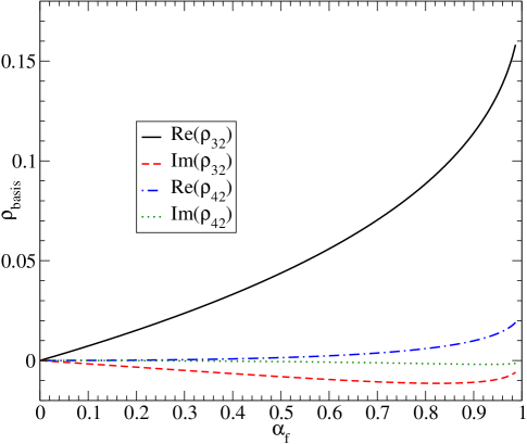
Figure 5: Real and imaginary parts of the mixing coefficients $\rho_{{\rm basis},32}$ and $\rho_{{\rm basis},42}$ for post-merger Kerr BHs of dimensionless spin $\alpha_{\rm f}$ (and corresponding fundamental $(2,2)$ QNM frequency $M_{\rm f}\sigma_{22}$). At the zero-spin limit $\alpha_{\rm f}\rightarrow 0$, the leakage vanishes.

We note here another manifestation of angular-basis mode-mixing demonstrated by Nuñez et al. Núñez et al. (2010). Those authors recast the Kerr perturbative problem using horizon-penetrating coordinates and with a novel (non-Kinnersley) null tetrad. On this background, they were able to show that the angular eigenfunctions are the (spin-weighted) spherical harmonics. However, the time-evolution of the radial mode functions for $(\ell,m)$ now involves the mode functions for terms $(\ell\pm 1,m)$ and $(\ell\pm 2,m)$.

III.3 Physical mixing

The discussion above exposes artifacts that arise from waveform decomposition using ordinary spin-weighted spherical harmonic functions. Here we ask whether, even with extraction spheres in the Boyer-Lindquist gauge, another decomposition using spin-weighted spheroidal harmonic functions can avoid mode-mixing.

The question is non-trivial. Although each leading-order quasinormal ringdown mode exhibits angular dependence described by some kind of spin-weighted spherical harmonic angular function, they are not mutually given by the same kind of spin-weighted spherical harmonic angular functions, since each has its own distinct quasinormal frequency $\sigma_{\ell m}$, and consequently a distinct preferred basis as labeled by $M\alpha\sigma=M_{\rm f}\alpha_{\rm f}\sigma_{\ell m}$. We must choose some particular orthonormal basis for the decomposition, and that basis cannot be simultaneously optimal for each mode.

That the spheroidal harmonics associated with different QNM frequencies are not perfectly orthogonal has been demonstrated for high-spin Kerr holes by Berti et al. Berti et al. (2006). To quantify this for a general end-state spin $\alpha_{\rm f}$, we define new overlaps $t_{\ell^{\prime}\ell}$, between spheroidal harmonics associated with different $m=2$ QNM frequencies:

$$t_{\ell^{\prime}\ell}=\oint d\Omega\,_{-2}\mathcal{Y}_{\ell}^{2}(M_{\rm f}\alpha_{\rm f}\sigma_{\ell 2})\,_{-2}\mathcal{Y}_{\ell}^{2}(M_{\rm f}\alpha_{\rm f}\sigma_{\ell^{\prime}2})^{*}.$$ (15)

”The upper panel of Fig. 6 shows the magnitude of these overlaps for $\ell=2$ and several values of $\ell^{\prime}$, while the lower panel shows the same for $\ell=3$. From these plots, we see that the spheroidal harmonics for different $M\alpha\sigma$ are not orthogonal, but show mixing by as much as $\approx 4\%$ for high spins (though the maximum overlaps occur at sub-maximal spins, as noted by Berti et al. (2006)). The overlaps are also greatest for “nearest neighbor” modes: $\ell=\ell^{\prime}\pm 1$. For example, if we decomposed a waveform, including a non-trivial $(2,2)$ QNM, in the spheroidal basis corresponding to the $(3,2)$ mode ringdown frequency, then the corresponding curve in Fig. 6 would represent a mixing coefficient analogous to those in the previous subsections. There is no choice of orthonormal basis that will avoid all such mode mixing. In this sense, the angular non-orthogonality of the quasinormal mode implies a form of physical mode-mixing, meaning that we can not perfectly isolate the QNM frequencies by any choice of angular basis.

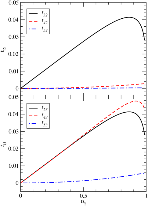
Figure 6: [Top panel] Magnitude of overlap $t_{\ell 2}$ between $\,{}_{-2}\mathcal{Y}_{2}^{2}$, evaluated at $M\alpha\sigma=M_{\rm f}\alpha_{\rm f}\sigma_{22}$ and $\,{}_{-2}\mathcal{Y}_{\ell}^{2}$, evaluated at $M\alpha\sigma=M_{\rm f}\alpha_{\rm f}\sigma_{\ell 2}$. [Bottom panel] Same for overlap $t_{\ell 3}$ between $\,{}_{-2}\mathcal{Y}_{3}^{2}$ and $\,{}_{-2}\mathcal{Y}_{\ell}^{2}$. By definition, $|t_{32}|=|t_{23}|$.

Fortunately it seems that the most evident mixing involves the dominant $(2,2)$ mode frequency bleeding into higher-$\ell$ modes. With that assumption we may still eliminate most physical mixing by choosing the basis compatible with this dominant quasinormal mode. If we decompose with the basis labeled by $M\alpha\sigma=M_{\rm f}\alpha_{\rm f}\sigma_{22}$ then the orthogonality of this particular basis will completely prevent the $(2,2)$ quasinormal mode from mixing into any other decomposed modal waveform component. In this way we can eliminate any “physical mixing” of the particular form described in Sec. II. Mixing among subdominant modes, or mixing of subdominant modes into the decomposed $(2,2)$ waveform component will still occur at some level, but this is a smaller effect, which we do not focus on in this paper.

IV Simulations

To investigate the mixing in a systematic way, we have surveyed several existing simulations of aligned-spin binaries, as well as carrying out new short simulations with the Goddard Hahndol evolution code. We choose our new black-hole binary (BHB) configurations in several groups of “merger-equivalent” classes, as described in Appendix B. The initial parameters for all these simulations, old and new, are presented in Table 1. In Fig. 7, we show the distribution of these configurations as plots in the two-dimensional configuration-spaces $\{\alpha_{1},\alpha_{2}\}$ and $\{\alpha_{1},q\}$, where $q\equiv M_{1}/M_{2}>1$ is the mass ratio, and $\alpha_{A}\equiv S_{A}/M_{A}^{2}$ is the dimensionless spin parameter of hole $A$, with physical values restricted to $\alpha_{A}\in[-1,1]$. Many of the longer and higher-resolution evolutions have appeared in previous publications Baker et al. (2008); Kelly et al. (2011). Since our primary interest here is strictly in the late-merger regime, newer evolutions begin only a few orbits before merger.

Table 1: Physical and numerical parameters of the initial data for all the runs presented. $m_{1,p}$ and $m_{2,p}$ are the bare puncture masses of the two pre-merger holes. $r_{0}$ is the initial coordinate separation, while $P_{0t}$ and $P_{0r}$ are the initial transverse and radial components of the Bowen-York linear momentum. $M_{\rm ADM}$ is the total energy of the initial data, while the total infinite-separation mass of the system is estimated by the sum of the initial Arnowitt-Deser-Misner (ADM) masses of the individual holes Baker (2002). We have found that for all cases here, this differs from the sum of apparent-horizon masses (calculated at times between $t=100$ and $200$), by less than a tenth of a percent.

run name	$m_{1,p}$	$m_{2,p}$	$S_{1z}$	$S_{2z}$	$r_{0}$	$P_{0t}$	$P_{0r}$	$M_{\rm ADM}$	$\sum_{i}M_{{\rm ADM},i}$
						$(\times 10^{2})$	$(\times 10^{4})$
X1_UU	0.301805	0.301805	0.2	0.2	8.20	10.32	0.00	0.988459	1.000804
X1_uu	0.454575	0.454575	0.1	0.1	10.21	9.25	9.17	0.99223	1.002768
X1_00	0.487231	0.487231	0.0	0.0	11.00	9.01	7.09	0.990514	1.000050
X1_UD	0.301805	0.301805	0.2	-0.2	11.00	9.01	7.09	0.990024	0.999222
X1.5_00	0.581359	0.380645	0.0	0.0	7.12	11.75	29.17	0.987252	1.000000
X1.75_00	0.619237	0.345598	0.0	0.0	7.42	11.01	24.10	0.988129	1.000000
X2_00	0.649344	0.314904	0.0	0.0	7.00	11.00	0.00	0.987939	1.000000
X2_DU	0.648662	0.265507	-0.066666667	0.066666667	10.00	8.52	7.63	0.990951	1.000009
X2.5_00	0.699349	0.269501	0.0	0.0	7.40	9.79	20.53	0.989664	1.000000
X3_00	0.738687	0.237505	0.0	0.0	8.88	7.88	8.96	0.991673	1.000000
X4_00	0.790000	0.189000	0.0	0.0	8.47	6.96	0.00	0.992912	1.000310
X5_U0	0.822007	0.157080	0.065083333	0.0	8.68	5.91	4.88	0.993733	1.000000
X3_d0	0.731667	0.237705	-0.087566063	0.0	9.06	7.84	8.76	0.99187	1.000000
X2_D0	0.587677	0.317821	-0.210380889	0.0	8.44	9.93	16.53	0.989967	1.000000
X1_DD	0.390411	0.390411	-0.159125	-0.159125	11.98	8.84	1.20	0.990453	0.998786
X5_00	0.824897	0.157031	0.0	0.0	8.67	5.97	5.85	0.993827	1.000000
X6_00	0.848615	0.133064	0.0	0.0	7.55	5.84	6.94219	0.994008	1.000000
X5_D0	0.822405	0.156318	-0.052232639	0.0	8.09	6.32	7.00085	0.993556	1.000000
X4_D0	0.778549	0.188766	-0.1213184	0.0	8.57	7.04	7.78076	0.992926	1.000000
X3_D0	0.692530	0.237756	-0.21614625	0.0	9.17	7.93	8.80172	0.99219	1.000000
X2_DD	0.531347	0.260245	-0.277766667	-0.069441667	10.72	8.56	7.81844	0.992008	1.000000

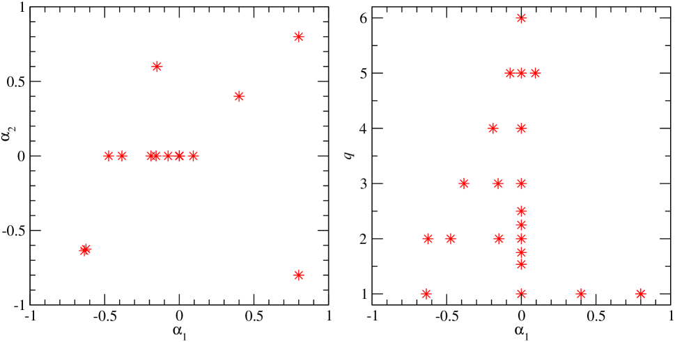
Figure 7: Simulated configurations from Table 1, represented as points in two-dimensional $\{\alpha_{1},\alpha_{2}\}$-space [left panel] and $\{\alpha_{1},q\}$-space [right panel]. Note that some points are associated with multiple simulations.

IV.1 Numerics

The initial momenta of the newer evolutions were chosen by integrating the post-Newtonian equations of motion, as outlined in Husa et al. (2008); Campanelli et al. (2009), with spin contributions to the Hamiltonian adapted from Buonanno et al. (2006); Damour et al. (2008); Porto and Rothstein (2006); Steinhoff et al. (2008a); Porto and Rothstein (2008); Steinhoff et al. (2008b), and the flux from Blanchet et al. (2006). Note that we did not attempt to reduce the eccentricity through tuning the initial momenta.

The new evolutions use the Hahndol code paired with the “Curie”release of the Einstein Toolkit Löffler et al. (2012), incorporating the Cactus Computational Toolkit cac and the Carpet mesh-refinement driver car .

In all cases, the initial data are of the standard Brandt-Brügmann puncture type Brandt and Brügmann (1997), using the Bowen-York Bowen and York Jr. (1980) prescription for extrinsic curvature that exactly satisfies the momentum constraint. We solve the remaining Hamiltonian constraint using the TwoPunctures spectral code Ansorg et al. (2004).

To evolve these initial data, we employ the BSSNOK 3+1 decomposition of Einstein’s vacuum equations Nakamura et al. (1987); Shibata and Nakamura (1995); Baumgarte and Shapiro (1999), with the alternative conformal variable $W\equiv e^{-2\phi}$ suggested in van Meter (2006); Tichy and Marronetti (2007); Marronetti et al. (2008), constraint-damping terms suggested in Duez et al. (2004), and the dissipation terms suggested in Kreiss and Oliger (1973); Hübner (1999). Our gauge conditions are the specific 1+log lapse and Gamma-driver shift described in van Meter et al. (2006), which constitute a variant of the now-standard “moving punctures” approach Campanelli et al. (2006a); Baker et al. (2006a). Our spatial derivatives use sixth-order-accurate differencing stencils, with the exception of advection derivatives, where we use fifth-order-accurate mesh-adapted differencing (MAD) Baker and van Meter (2005). Our time-integration is performed with a fourth-order Runge-Kutta algorithm.

IV.2 Waveform Extraction

We extract the gravitational waveforms from the simulations through the radiative Weyl scalar $\psi_{4}$ Baker et al. (2002a). This is evaluated throughout the grid, and interpolated onto a set of coordinate spheres at extraction radii $r\in[40M,90M]$. Over each sphere, the interpolant is integrated against the set of spin-weighted spherical harmonics $\,{}_{-2}Y_{\ell}^{m}(\theta,\phi)$, up to $\ell=5$.

In the extraction region, the grid spacing is between $M/2$ and $2M$, depending on the central resolution of the simulation. This is generally too coarse to resolve higher-frequency (and higher-$m$) modes with accuracy. Even for the dominant, relatively low-frequency, $(2,\pm 2)$ modes, dissipation effects are visible that spoil the $1/r$ extrapolation near and after merger. For this reason, we have used an $r$-extrapolation scheme that includes an explicit dissipative term in the amplitude of each mode:

$$A_{\ell m}(r)=a_{-1}r+a_{0}+a_{2}r^{-2},\;\;\varphi_{\ell m}(r)=b_{0}+b_{2}r^{-2}.$$

We have found this extrapolation procedure to be robust only for the higher-resolution simulations in this paper.

As a result, a waveform-derived quantity $f$ will have errors due to finite extraction radius and finite resolution. For this paper, we make a very conservative error estimate by adding uncertainties linearly:

$$\Delta f=\Delta_{r}f+\Delta_{h}f.$$

For the finite-$r$ error, we assume an uncertainty equal to the difference between the coefficient from the $r$-extrapolated highest-resolution data and that measured from the largest finite-$r$ data at the same resolution. For finite-resolution error, we use the difference between the same-extraction-radius data at the coarse and fine resolutions as our estimate of the error in the fine-resolution result. For many configurations, we only have a single resolution available and the r-extrapolation is not reliable at this resolution. For these, we adopt a conservative overall error estimate by taking the average error from comparable two-resolution configurations and multiply it by 1.5. For amplitudes, this is a relative error, while for phase measurements, it is the absolute error.

V Analysis of Waveforms

Using the ringdown data from all the simulations in Sec. IV, we performed least-squares fits to the real part of the strain-rate $(2,2)$ and $(3,2)$ waveforms, using the forms of Eqs. (1)-(2). Our fit is over the window $t\in[20,55]$, where $t=0$ is the time of peak $(2,2)$ mode amplitude. By starting $20M$ after peak amplitude, we ensure that we are in the linear ringdown regime; by stopping at $55M$, we avoid the low-amplitude degradation seen in late-ringdown waveforms. As the tabulated version of the results would be excessively long, we present our raw results purely graphically.

We begin by showing the nature of the complex numerical “leakage parameter” derived from the ratio of fitted parameters from the measured $(2,2)$ and $(3,2)$ modes during ringdown, using (1)-(2):

$$\rho_{{\rm num},32}\equiv\frac{\rho_{32}A_{22}e^{i(\sigma_{22}t+\delta_{22})}}{A_{22}e^{i(\sigma_{22}t+\delta_{22})}}.$$ (16)

Figure 8 shows the real and imaginary parts of this leakage for all configurations presented in this paper, as a function of the dimensionless spin $\alpha_{\rm f}$ of the post-merger hole.

V.1 Comparing Hypotheses

In Sec. III we discussed two possible causes for mode-mixing effects of the form

$$\dot{h}_{(\ell,2)}^{\rm model}=A_{\ell 2}e^{i(\sigma_{\ell 2}t+\delta_{\ell 2})}+\rho_{\ell 2}A_{22}e^{i(\sigma_{22}t+\delta_{22})},$$ (17)

described in Sec. II. If the mixing is caused by BMS supertranslation gauge ambiguity, then we would expect nearly pure imaginary $\rho_{\ell 2}$. On the other hand, if the mixing derives from the distinction between spheroidal and spherical harmonic angular functions, then we expect predominantly real $\rho_{\ell 2}$ of a quantified size. In Fig. 8 we see that the argument of $\rho_{{\rm num},32}$ is close to zero, within error bars for most cases, making $\rho_{{\rm num},32}$ predominantly real, consistent with the spheroidal harmonic hypothesis. The largest deviations from zero are also those with the largest uncertainties arising from the QNM fit process.

The analysis of Sec. III.1 suggests that a change of supertranslation gauge would give rise to mode-mixing coefficients with a numerically significant imaginary part in the measured waveform. Since the imaginary part of $\rho_{{\rm num},32}$ is so small, any supertranslation gauge effects are negligible at the level of interest here. We can estimate the degree of gauge constraint implied by a null measurement of this effect. From the bottom panel of Fig. 8, one sees that the imaginary component of the mixing coefficient $\rho_{{\rm num},32}$ is constrained to values within $\pm 0.02$ in almost all cases. If we generously assumed that all of this imaginary mixing was caused by gauge distortion of the extraction sphere, by comparison with Fig. 4, we would conclude that the amplitude of the distortion ($b_{20}$ specifically) would have to be smaller than about $0.2M$, suggesting a remarkable level of supertranslation gauge optimality in these simulations.

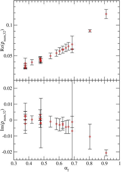
Figure 8: Real [top panel] and imaginary [bottom panel] parts of complex leakage parameter $\rho_{{\rm num},32}$ (16), shown as a function of $\alpha_{\rm f}$, the dimensionless spin of the post-merger hole for all runs, indicating that in almost all cases, the leakage parameter is predominantly real.

V.2 Testing the Spheroidal Leakage Model

We have seen that the numerical results for the complex argument of $\rho_{32}$ are consistent with the spherical-spheroidal mixing hypothesis, but this hypothesis also makes quantitative predictions for the magnitude $\left|\rho_{32}\right|$. In the top panel of Fig. 9, we plot the magnitude of $\rho_{{\rm num},32}$ as a function of $\alpha_{\rm f}$. We overlay these points with the magnitude of the leakage coefficients $\rho_{{\rm basis},32}$ (14) plotted in Fig. 5 (blue solid curve). From the close fit, it appears that the leakage is in fact dominated by this spheroidal/spherical harmonic mismatch. That is, even though the post-merger background coordinate system should not be expected to closely resemble the Kerr-Boyer-Lindquist slicing assumed by Teukolsky’s perturbative work, nevertheless, this expected warping is not as important as our choice of harmonic basis functions.

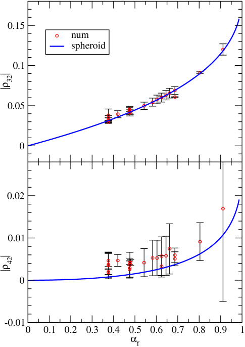
Figure 9: [Top panel] Amplitude of measured $(2,2)\rightarrow(3,2)$ leakage parameter $\rho_{{\rm num},32}$ as a function of $\alpha_{\rm f}$, the dimensionless spin of the post-merger hole for all runs. The curve is the theoretical ratio $\rho_{{\rm basis},32}$ due to spheroidal-spherical leakage. [Bottom panel] Same for $(2,2)\rightarrow(4,2)$ leakage ratio $\rho_{{\rm num},42}$.

The bottom panel of Fig. 9 shows the complex amplitude of the equivalent parameter $\rho_{{\rm num},42}$ governing the leakage of the $(2,2)$ mode into the measured $(4,2)$ mode. Although this is also consistent with expectations from angular-basis mixing (blue solid curve), the relative errors swamp the numerical data, and higher-resolution numerics will be needed to establish the relation unambiguously.

V.3 Finding the Residual $(3,2)$ Mode Amplitude

If we regard the measured $(3,2)$ mode as the combination of a “true” $(3,2)$ mode $A_{32}\exp{i(\sigma_{32}t+\delta_{\ell 2})}$ and a piece of the $(2,2)$ mode, we may ask whether we can model the residual $(3,2)$ contribution. When looking at the entire suite of simulations, it is difficult to see a distinct pattern in these true $(3,2)$ amplitudes. However, it is instructive to carry out a particular slice in configuration space.

In Fig. 10, we show a subset of the $(3,2)$ amplitudes formed by the mergers of nonspinning binaries, with mass ratio $q\equiv M_{1}/M_{2}\in\{1.0,6.0\}$. Error bars in this plot have been estimated in the same way as for Fig. 9. Clearly the high-$q$ behavior seems to decay to some constant amplitude, while there is some local minimum around $\eta=0.21$ (between $q=2$ and $q=2.25$), indicating that perhaps at this mass-ratio, the $(3,2)$ QNM is hardly excited at all.

We also present an empirical fit to this data of the functional form

$$A_{32}(\eta)=\sqrt{\left(a-be^{-\lambda/\eta}\right)^{2}+c^{2}},$$ (18)

where the parameters take the values $a=0.0147\pm 0.0002$, $b=1.5\pm 0.1$, $c=0.0026\pm 0.0002$, and $\lambda=0.98\pm 0.02$. Fits of this form are expected to be useful for generating merger template waveforms for the subdominant modes.

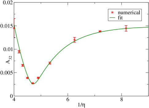
Figure 10: Corrected amplitude $A_{32}$ of the $(3,2)$ strain-rate mode for nonspinning binaries with mass ratio $q\in\{1.0,6.0\}$. The solid (green) curve is a fit to these points of the functional form (18).

VI Discussion

In this paper, we have investigated “bumps” measured in the merger-ringdown portion of certain gravitational-radiation angular waveform modes from the numerical simulation of the coalescence of black-hole binaries (BHBs). These bumpy modes appear to contain significant contributions from the dominant $(2,2)$ mode, indicating some kind of mode-mixing at work.

We have considered three classes of effects that may contribute to mode-mixing in numerically extracted and decomposed merger-ringdown waveforms. These are: gauge effects, arising from supertranslation gauge freedom for outgoing radiation in general asymptotically flat spacetimes (see Sec. III.1); angular-basis effects, relating to a choice between spin-weighted spherical or quasinormal-mode-adapted spheroidal harmonic bases (Sec. III.2); and physical quasinormal-mode mixing effects that are independent of any representation changes (Sec. III.3).

We have identified and analyzed the measured mode-mixing bumps in the most prominent of the bumpy gravitational waveform modes modes — $\ell=3$,$m=2$ — measured from a set of numerical evolutions of aligned-spin BHB mergers. Our analysis has allowed us to distinguish between the contributions of our three mode-mixing effects. We find that the angular-basis effects dominate. Although other kinds of effects may be present – like the frequency-dependent gauge supertranslations discussed in Sec. III.1 – they cannot be seen clearly here with the level of accuracy available from our current simulations.

In this way our analysis further codifies the results from the ringdown stage of the aligned-spin mergers. This was originally prompted by our work on a multi-mode waveform model based on the implicit rotating source (IRS) picture of black-hole merger Baker et al. (2008); Kelly et al. (2011). In this model, the dominant and leading subdominant waveform modes from binary mergers were seen to share a common rotational phase, with a corresponding rotational frequency that increased monotonically through inspiral and merger, reaching a plateau during ringdown. The corresponding mode amplitudes could be modeled by a simple, few-parameter functional form that depends on the frequency function, with a single well-defined peak. Attempting to extend this to the $(3,2)$ mode proved problematic, as the measured mode was no longer monotonic in frequency, or single-peaked in amplitude.

More broadly, we expect our results to provide guidance in the ongoing effort of combining results of analytic and numerical relativity studies toward the goal of a fully developed family of efficient and accurate black-hole merger waveforms. Because the comparison of waveform models is typically conducted mode by mode in decomposed form, the issues we have studied may lead to unnecessarily spurious features in particular waveform representations.

We estimate, for instance, that supertranslation gauge changes that would effectively distort the shape of arbitrarily large waveform-extraction spheres on scales of order $M_{\rm f}$ or smaller would be sufficient to qualitatively influence the mode-mixing features focused on in this study. The absence of such effects is itself intriguing, suggesting that we have achieved nearly optimal choice of supertranslation gauge. Our near-optimal spheroidal harmonic basis is consistent with quasinormal-mode distortions of Kerr space-time in the Boyer-Lindquist coordinate system. That we see negligible supertranslation mode-mixing suggests that the outer regions of our numerical space-times asymptotically approach distorted Kerr in Boyer-Lindquist coordinates faster (in powers of $1/r$) than the asymptotic approach to perturbed Minkowski spacetime. This seems plausible, based on our choice of numerical gauge, which approximates maximal time slicing and $\tilde{\Gamma}^{i}=0$ spatial coordinates. The latter condition will yield spatially isotropic coordinates where possible.

Nonetheless, it seems that we have been lucky to stumble onto a near-optimal representation as other incompatible gauge choices may also be reasonable in the numerical simulation context. In continued pursuit of higher-precision waveform comparisons and higher-fidelity analytic models (see, e.g., the NR-AR project NRA ), we expect such considerations to grow in significance. (They may also be crucial in studies of how the pre-merger BHB configuration is encoded in the relative amplitude of different quasinormal modes during ringdown; see, e.g. Kamaretsos et al. (2012).) Similarly we find that physical mode-mixing among the quasinormal modes will prevent any orthonormal representation from fully separating frequencies at sufficiently high precision.

For simulations similar to ours, where gauge and physical mixing effects remain small, and the primary source of mixing involves the $(2,2)$ mode, our results suggest that decomposition with a spheroidal harmonic basis $\{\,_{-2}\mathcal{Y}_{\ell}^{m}(M_{f}\alpha_{f}\sigma_{22};\theta,\phi)\}$ may be close to an optimal basis for achieving modal frequency separation, and thus nearly beat-free waveforms.

It may be asked whether the conclusions drawn here can be applied to the pre-merger waveform signal. We know that the PN mode amplitudes (see, for instance, Eqs. (4.17) of Arun et al. (2009)) are dominated by the $(2,\pm 2)$ (quadrupole) spherical harmonic modes, with $(\ell>2,\pm 2)$ modes entering at higher PN order. It might be possible, in principle, to find a “best possible” effective background spin parameter $\alpha_{\rm eff}$ whose associated spheroidal harmonic basis would absorb most of these higher-$\ell$ modes; in practice, however, this would be numerically impractical at any fixed frequency, and of course, the frequency would change continuously during inspiral, as (presumably) would the spin, since the binary is constantly losing angular momentum.

Appendix A Calculating Spheroidal Harmonics

As there are no closed-form solutions for the $\,{}_{-2}\mathcal{Y}_{\ell}^{m}$, we must proceed numerically. While setting up the popular continued-fraction method for computing the quasinormal-mode (QNM) frequencies of a Kerr black hole, Leaver Leaver (1985) presents the following power-series expansion for the polar-angle function $\,{}_{-2}S_{\ell}^{m}(M\alpha\sigma;\cos\theta)$, due originally to Baber & Hassé Baber and Hassé (1935) (we specialize here to $s=-2$):

$$\,{}_{-2}S_{\ell}^{m}(M\alpha\sigma;x)= e^{M\alpha\sigma x}(1+x)^{|m+2|/2}(1-x)^{|m-2|/2}$$

$$\times\sum_{n=0}^{\infty}a_{n}(1+x)^{n},$$ (19)

where the expansion coefficients $a_{n}$ are determined up to an overall scaling — the value of $a_{0}$ — by the same recurrence relations that yield the QNM frequencies. For our desired Kerr spin $\alpha_{\rm f}$, we first determine the (complex) fundamental QNM frequency of the $(2,2)$ mode, $M_{\rm f}\sigma_{22}$. Next, assuming $a_{0}=1$, we use the recurrence relations from Leaver (1985) to determine the $a_{n}$ (in practice, we truncate the series at $n=14$). Requiring that

$$\int_{-1}^{1}dx\left|\,{}_{-2}S_{\ell}^{m}(M_{\rm f}\alpha_{\rm f}\sigma_{22};x)\right|^{2}=1$$

then fixes $a_{0}$, supplying the correct normalization of the $a_{n}$.

Appendix B Kerr-Equivalent Black-Hole Binaries

The end-point of any merger of BHBs in vacuum is expected to be a single Kerr black hole, parametrized by two numbers, the mass $M_{\rm f}$ and spin angular momentum $\vec{S}_{\rm f}=\alpha_{\rm f}M_{\rm f}^{2}$. These should satisfy the global conservation rules:

$$M_{\rm f} =M_{\rm ADM}-E_{\rm rad},$$ (20)

$$\vec{S}_{\rm f} =\vec{J}_{\rm ADM}-\vec{J}_{\rm rad},$$ (21)

where $M_{\rm ADM}$ and $\vec{J}_{\rm ADM}$ are the Arnowitt-Deser-Misner (ADM) energy and total angular momentum of the initial data, and $E_{\rm rad}$ and $\vec{J}_{\rm rad}$ are the energy and angular momentum emitted in gravitational radiation during the course of the evolution.

Fixing the initial separation of the binary, and taking its total mass to be $M=M_{1}+M_{2}$ ($>M_{\rm ADM}$ for any finite initial separation), and assuming zero eccentricity, the black-hole binary will have seven free parameters: $\{q,\vec{S}_{1},\vec{S}_{2}\}$, where $q\equiv M_{1}/M_{2}>1$ is the mass ratio, and $\vec{S}_{A}$ are the spin angular momentum vectors of the two holes. However, the end-state has just two parameters: $\{M_{\rm f},\vec{S}_{\rm f}\}$, so there must be a large degeneracy in the initial parameters.

Viewing the BHB coalescence as a kind of simple particle interaction, Boyle et al. Boyle and Kesden (2008) used symmetry arguments to restrict the possible end-states of the BHB merger. This is the basis of end-state formulae by Tichy & Marronetti Tichy and Marronetti (2008). Other models have been developed by Buonanno et al.  Buonanno et al. (2008), Lousto et al. Lousto et al. (2010b), Barausse & Rezzolla Rezzolla et al. (2008); Barausse and Rezzolla (2009), and others.

In the case of initially orbit-aligned spins, the initial parameter space is three-dimensional: $\{q,S_{1},S_{2}\}$. We use the simplest applicable formulas for the achieved end-state for an aligned-spin system. The end-state mass formula we take from Eq. (5) of Lousto et al. (2010b):

$$M_{\rm f} =1-\eta E_{\rm ISCO}-E_{2}\eta^{2}-E_{3}\eta^{3}$$

$$-\frac{\eta^{2}}{(1+q)^{2}}\left[E_{S}(\alpha_{2}+q^{2}\alpha_{1})+E_{\delta}(1-q)(\alpha_{2}-q\alpha_{1})\right.$$

$$\left.+E_{A}(\alpha_{2}+q\alpha_{1})^{2}+E_{D}(\alpha_{2}-q\alpha_{1})^{2}\right],$$ (22)

where $\eta\equiv M_{1}M_{2}/(M_{1}+M_{2})^{2}=q/(1+q)^{2}$ is the symmetric mass ratio of the binary, and the fitting parameters are:

$$E_{\rm ISCO}= 1-\frac{\sqrt{8}}{3}+0.103803\eta+\frac{(q(1+2q)\alpha_{1}+(2+q)\alpha_{2})}{36\sqrt{3}(1+q)^{2}}$$

$$+\frac{5(q\alpha_{1}-\alpha_{2})^{2}}{162\sqrt{2}(1+q)^{2}},$$

$$E_{2}= 0.341,\;\;E_{3}=0.522,\;\;E_{S}=0.673,$$

$$E_{\delta}= -0.36,\;\;E_{A}=-0.014,\;\;E_{D}=0.26.$$

For the final spin, one model with just enough complexity for our data sets here was given by Rezzolla et al. (2008); Barausse and Rezzolla (2009) :

$$\alpha_{\rm f}=\tilde{\alpha}+s_{4}\eta\tilde{\alpha}^{2}+s_{5}\eta^{2}\tilde{\alpha}+t_{0}\eta\tilde{\alpha}+2\sqrt{3}\eta+t_{2}\eta^{2}+t_{3}\eta^{3},$$ (23)

where $\tilde{\alpha}\equiv(q^{2}\alpha_{1}+\alpha_{2})/(q^{2}+1)$ and the coefficients $\{s_{4},s_{5},t_{0},t_{2},t_{3}\}$ are:

$$s_{4} =-0.1229\pm 0.0075,\;s_{5}=0.4537\pm 0.1463,$$

$$t_{0} =-2.8904\pm 0.0359,\;t_{2}=-3.5171\pm 0.1210,$$

$$t_{3} =2.5763\pm 0.4833.$$

Using these formulae, we have constructed a set of configurations, which we present in Table 1, grouped by final Kerr spin.

Table 2: Final mass and spin of the post-merger Kerr BH, as measured by radiation balance ($M_{\rm f}$, $\alpha_{\rm f}$), and as predicted by phenomenological equations (22)-(23) ($M_{\rm f,RIT}$,$\alpha_{\rm f,AEI}$). The final two columns give the percentage relative error between the measured and predicted values, which never exceeds 1.6 % for the mass and 2.1 % for the spin.

run name	$M_{\rm f}$	$\alpha_{\rm f}$	$M_{\rm f,RIT}$	$\alpha_{\rm f,AEI}$	$\delta M_{\rm f}$ (%)	$\delta\alpha_{\rm f}$ (%)
X1_UU	0.9156	0.9053	0.9287	0.9112	1.43	0.65
X1_uu	0.9393	0.8119	0.9391	0.8038	0.03	0.99
X1_00	0.9520	0.6886	0.9497	0.6865	0.24	0.31
X1_UD	0.9505	0.6839	0.9359	0.6865	1.54	0.38
X1.5_00	0.9558	0.6664	0.9534	0.6644	0.25	0.30
X1.75_00	0.9588	0.6475	0.9565	0.6452	0.24	0.35
X2_00	0.9614	0.6254	0.9596	0.6244	0.19	0.17
X2_DU	0.9610	0.6120	0.9559	0.6244	0.54	2.02
X2.5_00	0.9671	0.5833	0.9654	0.5824	0.18	0.16
X3_00	0.9716	0.5432	0.9702	0.5429	0.15	0.07
X4_00	0.9782	0.4780	0.9812	0.4748	0.31	0.68
X5_U0	0.9816	0.4741	0.9773	0.4748	0.44	0.15
X3_d0	0.9737	0.4735	0.9720	0.4760	0.18	0.52
X2_D0	0.9683	0.4704	0.9649	0.4765	0.35	1.31
X1_DD	0.9646	0.4825	0.9674	0.4786	0.30	0.81
X5_00	0.9826	0.4186	0.9821	0.4202	0.06	0.37
X6_00	0.9857	0.3718	0.9854	0.3762	0.02	1.18
X5_D0	0.9834	0.3736	0.9791	0.3762	0.44	0.68
X4_D0	0.9803	0.3728	0.9791	0.3762	0.13	0.91
X3_D0	0.9762	0.3697	0.9739	0.3762	0.23	1.75
X2_DD	0.9718	0.3788	0.9729	0.3762	0.11	0.71

References

- Pretorius (2005) F. Pretorius, Phys. Rev. Lett. 95, 121101 (2005), eprint arXiv:gr-qc/0507014.
- Campanelli et al. (2006a) M. Campanelli, C. O. Lousto, P. Marronetti, and Y. Zlochower, Phys. Rev. Lett. 96, 111101 (2006a), eprint arXiv:gr-qc/0511048.
- Baker et al. (2006a) J. G. Baker, J. M. Centrella, D.-I. Choi, M. Koppitz, and J. R. van Meter, Phys. Rev. Lett. 96, 111102 (2006a), eprint arXiv:gr-qc/0511103.
- Baker et al. (2007) J. G. Baker, M. Campanelli, F. Pretorius, and Y. Zlochower, Class. Quantum Grav. 24, S25 (2007), eprint arXiv:gr-qc/0701016.
- Hannam et al. (2009) M. D. Hannam, S. Husa, J. G. Baker, M. Boyle, B. Brügmann, T. Chu, E. N. Dorband, F. Herrmann, I. Hinder, B. J. Kelly, et al., Phys. Rev. D 79, 084025 (2009), eprint arXiv:0901.2437 [gr-qc].
- Campanelli et al. (2006b) M. Campanelli, C. O. Lousto, and Y. Zlochower, Phys. Rev. D 74, 041501(R) (2006b), eprint arXiv:gr-qc/0604012.
- Buonanno et al. (2007) A. Buonanno, G. B. Cook, and F. Pretorius, Phys. Rev. D 75, 124018 (2007), eprint arXiv:gr-qc/0610122.
- Boyle et al. (2007) M. Boyle, D. A. Brown, L. E. Kidder, A. H. Mroué, H. P. Pfeiffer, M. A. Scheel, G. B. Cook, and S. A. Teukolsky, Phys. Rev. D 76, 124038 (2007), eprint arXiv:0710.0158 [gr-qc].
- Scheel et al. (2009) M. A. Scheel, M. Boyle, T. Chu, L. E. Kidder, K. D. Matthews, and H. P. Pfeiffer, Phys. Rev. D 79, 024003 (2009), eprint arXiv:0810.1767 [gr-qc].
- González et al. (2009) J. A. González, U. Sperhake, and B. Brügmann, Phys. Rev. D 79, 124006 (2009), eprint arXiv:0811.3952 [gr-qc].
- Lousto et al. (2010a) C. O. Lousto, H. Nakano, Y. Zlochower, and M. Campanelli, Phys. Rev. Lett. 104, 211101 (2010a), eprint arXiv:1001.2316 [gr-qc].
- Centrella et al. (2010) J. M. Centrella, J. G. Baker, B. J. Kelly, and J. R. van Meter, Rev. Mod. Phys. 82, 3069 (2010), eprint arXiv:1010.5260 [gr-qc].
- Hinder (2010) I. Hinder, Class. Quantum Grav. 27, 114004 (2010), invited paper from Numerical Relativity and Data Analysis (NRDA) 2009, Albert Einstein Institute, Potsdam, eprint arXiv:1001.5161 [gr-qc].
- Ajith et al. (2011) P. Ajith, M. D. Hannam, S. Husa, Y. Chen, B. Brügmann, E. N. Dorband, D. Müller, F. Ohme, D. Pollney, C. Reisswig, et al., Phys. Rev. Lett. 106, 241101 (2011), eprint arXiv:0909.2867 [gr-qc].
- Pan et al. (2010) Y. Pan, A. Buonanno, L. T. Buchman, T. Chu, L. E. Kidder, H. P. Pfeiffer, and M. A. Scheel, Phys. Rev. D 81, 084041 (2010), eprint arXiv:0912.3466 [gr-qc].
- Santamaría et al. (2010) L. Santamaría, F. Ohme, P. Ajith, B. Brügmann, E. N. Dorband, M. D. Hannam, S. Husa, P. Mösta, D. Pollney, C. Reisswig, et al., Phys. Rev. D 82, 064016 (2010), eprint arXiv:1005.3306 [gr-qc].
- Arun et al. (2007a) K. G. Arun, B. R. Iyer, B. S. Sathyaprakash, and S. Sinha, Phys. Rev. D 75, 124002 (2007a), eprint arXiv:0704.1086 [gr-qc].
- Arun et al. (2007b) K. G. Arun, B. R. Iyer, B. S. Sathyaprakash, S. Sinha, and C. Van Den Broeck, Phys. Rev. D 76, 104016 (2007b), eprint arXiv:0707.3920 [astro-ph].
- Trias and Sintes (2008) M. Trias and A. M. Sintes, Class. Quantum Grav. 25, 184032 (2008), 12th GWDAW (Gravitational Wave Data Analysis Workshop), eprint arXiv:0804.0492 [gr-qc].
- McWilliams et al. (2010) S. T. McWilliams, J. I. Thorpe, J. G. Baker, and B. J. Kelly, Phys. Rev. D 81, 064014 (2010), eprint arXiv:0911.1078 [gr-qc].
- Goldberg et al. (1967) J. N. Goldberg, A. J. MacFarlane, E. T. Newman, F. Rohrlich, and E. C. G. Sudarshan, J. Math. Phys. 8, 2155 (1967).
- Wiaux et al. (2007) Y. Wiaux, L. Jacques, and P. Vandergheynst, J. Comp. Phys. 226, 2359 (2007), eprint arXiv:astro-ph/0508514.
- Berti et al. (2007) E. Berti, V. Cardoso, J. A. González, U. Sperhake, M. D. Hannam, S. Husa, and B. Brügmann, Phys. Rev. D 76, 064034 (2007), eprint arXiv:gr-qc/0703053.
- Berti et al. (2008) E. Berti, V. Cardoso, J. A. González, U. Sperhake, and B. Brügmann, Class. Quantum Grav. 25, 114035 (2008), eprint arXiv:0711.1097 [gr-qc].
- Baker et al. (2008) J. G. Baker, W. D. Boggs, J. M. Centrella, B. J. Kelly, S. T. McWilliams, and J. R. van Meter, Phys. Rev. D 78, 044046 (2008), eprint arXiv:0805.1428 [gr-qc].
- Kelly et al. (2011) B. J. Kelly, J. G. Baker, W. D. Boggs, S. T. McWilliams, and J. M. Centrella, Phys. Rev. D 84, 084009 (2011), eprint arXiv:1107.1181 [gr-qc].
- Pan et al. (2011) Y. Pan, A. Buonanno, M. Boyle, L. T. Buchman, L. E. Kidder, H. P. Pfeiffer, and M. A. Scheel, Phys. Rev. D 84, 124052 (2011), eprint arXiv:1106.1021 [gr-qc].
- Baker et al. (2002a) J. G. Baker, M. Campanelli, and C. O. Lousto, Phys. Rev. D 65, 044001 (2002a), eprint arXiv:gr-qc/0104063.
- Baker et al. (2002b) J. G. Baker, M. Campanelli, C. O. Lousto, and R. Takahashi, Phys. Rev. D 65, 124012 (2002b), eprint arXiv:astro-ph/0202469.
- Baker et al. (2006b) J. G. Baker, J. M. Centrella, D.-I. Choi, M. Koppitz, and J. R. van Meter, Phys. Rev. D 73, 104002 (2006b), eprint arXiv:gr-qc/0602026.
- Schnittman et al. (2008) J. D. Schnittman, A. Buonanno, J. R. van Meter, J. G. Baker, W. D. Boggs, J. M. Centrella, B. J. Kelly, and S. T. McWilliams, Phys. Rev. D 77, 044031 (2008), eprint arXiv:0707.0301 [gr-qc].
- Bondi et al. (1962) H. Bondi, M. G. J. van der Burg, and A. W. K. Metzner, Proc. R. Soc. London Ser. A 269, 21 (1962).
- Sachs (1962) R. K. Sachs, Proc. R. Soc. London Ser. A 270, 103 (1962).
- Gualtieri et al. (2008) L. Gualtieri, E. Berti, V. Cardoso, and U. Sperhake, Phys. Rev. D 78, 044024 (2008), eprint arXiv:0805.1017 [gr-qc].
- Campanelli et al. (2009) M. Campanelli, C. O. Lousto, H. Nakano, and Y. Zlochower, Phys. Rev. D 79, 084010 (2009), eprint arXiv:0808.0713 [gr-qc].
- Schmidt et al. (2011) P. Schmidt, M. D. Hannam, S. Husa, and P. Ajith, Phys. Rev. D 84, 024046 (2011), eprint arXiv:1012.2879 [gr-qc].
- O’Shaughnessy et al. (2011) R. O’Shaughnessy, B. Vaishnav, J. Healy, Z. Meeks, and D. M. Shoemaker, Phys. Rev. D 84, 124002 (2011), eprint arXiv:1109.5224 [gr-qc].
- O’Shaughnessy et al. (2012) R. O’Shaughnessy, J. Healy, L. London, Z. Meeks, and D. M. Shoemaker, Phys. Rev. D 85, 084003 (2012), eprint arXiv:1201.2113 [gr-qc].
- Schmidt et al. (2012) P. Schmidt, M. D. Hannam, and S. Husa (2012), arXiv:1207.3088 [gr-qc].
- Vishveshwara (1970) C. V. Vishveshwara, Nature 227, 936 (1970).
- Press (1971) W. H. Press, Astrophys. J. 170, L105 (1971).
- Teukolsky (1972) S. A. Teukolsky, Phys. Rev. Lett. 29, 1114 (1972).
- Boyer and Lindquist (1967) R. H. Boyer and R. W. Lindquist, J. Math. Phys. 8, 265 (1967).
- Campanelli et al. (2001) M. Campanelli, G. Khanna, P. Laguna, J. A. Pullin, and M. P. Ryan, Class. Quantum Grav. 18, 1543 (2001), eprint arXiv:gr-qc/0010034.
- Núñez et al. (2010) D. Núñez, J. C. Degollado, and C. Palenzuela, Phys. Rev. D 81, 064011 (2010), eprint arXiv:1002.2227 [gr-qc].
- Berti et al. (2006) E. Berti, V. Cardoso, and M. Casals, Phys. Rev. D 73, 024013 (2006), Erratum: ibid. 73, 109902(E) (2006), eprint arXiv:gr-qc/0511111.
- Baker (2002) B. D. Baker (2002), arXiv:gr-qc/0205082.
- Husa et al. (2008) S. Husa, M. D. Hannam, J. A. González, U. Sperhake, and B. Brügmann, Phys. Rev. D 77, 044037 (2008), eprint arXiv:0706.0904 [gr-qc].
- Buonanno et al. (2006) A. Buonanno, Y. Chen, and T. Damour, Phys. Rev. D 74, 104005 (2006), eprint arXiv:gr-qc/0508067.
- Damour et al. (2008) T. Damour, P. Jaranowski, and G. Schäfer, Phys. Rev. D 77, 064032 (2008), eprint arXiv:0711.1048 [gr-qc].
- Porto and Rothstein (2006) R. A. Porto and I. Z. Rothstein, Phys. Rev. Lett. 97, 021101 (2006), eprint arXiv:gr-qc/0604099.
- Steinhoff et al. (2008a) J. Steinhoff, S. Hergt, and G. Schäfer, Phys. Rev. D 77, 081501(R) (2008a), eprint arXiv:0712.1716 [gr-qc].
- Porto and Rothstein (2008) R. A. Porto and I. Z. Rothstein, Phys. Rev. D 78, 044013 (2008), Errata: ibid. 81, 029904(E) (2010); 81, 029905(E) (2010), eprint arXiv:0804.0260 [gr-qc].
- Steinhoff et al. (2008b) J. Steinhoff, S. Hergt, and G. Schäfer, Phys. Rev. D 78, 101503(R) (2008b), eprint arXiv:0809.2200 [gr-qc].
- Blanchet et al. (2006) L. Blanchet, A. Buonanno, and G. Faye, Phys. Rev. D 74, 104034 (2006), Errata: ibid. 75, 049903(E) (2007); 81, 089901(E) (2010), eprint arXiv:gr-qc/0605140.
- Löffler et al. (2012) F. Löffler, J. Faber, E. Bentivegna, T. Bode, P. Diener, R. Haas, I. Hinder, B. C. Mundim, C. D. Ott, E. Schnetter, et al., Class. Quantum Grav. 29, 115001 (2012), eprint arXiv:1111.3344 [gr-qc].
- (57) Cactus computational toolkit home page, http://www.cactuscode.org.
- (58) Carpet: Adaptive Mesh Refinement for the Cactus Framework, http://www.carpetcode.org/.
- Brandt and Brügmann (1997) S. R. Brandt and B. Brügmann, Phys. Rev. Lett. 78, 3606 (1997), eprint arXiv:gr-qc/9703066.
- Bowen and York Jr. (1980) J. M. Bowen and J. W. York Jr., Phys. Rev. D 21, 2047 (1980).
- Ansorg et al. (2004) M. Ansorg, B. Brügmann, and W. Tichy, Phys. Rev. D 70, 064011 (2004), eprint arXiv:gr-qc/0404056.
- Nakamura et al. (1987) T. Nakamura, K.-I. Oohara, and Y. Kojima, Prog. Theor. Phys. Suppl. 90, 1 (1987).
- Shibata and Nakamura (1995) M. Shibata and T. Nakamura, Phys. Rev. D 52, 5428 (1995).
- Baumgarte and Shapiro (1999) T. W. Baumgarte and S. L. Shapiro, Phys. Rev. D 59, 024007 (1999), eprint arXiv:gr-qc/9810065.
- van Meter (2006) J. R. van Meter, in From Geometry to Numerics (Institut Henri Poincaré, Paris, 2006), http://luth2.obspm.fr/IHP06/workshops/geomnum/slides/vanmeter.pdf.
- Tichy and Marronetti (2007) W. Tichy and P. Marronetti, Phys. Rev. D 76, 061502(R) (2007), eprint arXiv:gr-qc/0703075.
- Marronetti et al. (2008) P. Marronetti, W. Tichy, B. Brügmann, J. A. González, and U. Sperhake, Phys. Rev. D 77, 064010 (2008), eprint arXiv:0709.2160[gr-qc].
- Duez et al. (2004) M. D. Duez, S. L. Shapiro, and H.-J. Yo, Phys. Rev. D 69, 104016 (2004), eprint arXiv:gr-qc/0401076.
- Kreiss and Oliger (1973) H.-O. Kreiss and J. Oliger, Methods for the approximate solution of time dependent problems, no. 10 in GARP Publications Series (World Meteorological Organization and International Council of Scientific Unions, Geneva, 1973).
- Hübner (1999) P. Hübner, Class. Quantum Grav. 16, 2823 (1999), eprint arXiv:gr-qc/9903088.
- van Meter et al. (2006) J. R. van Meter, J. G. Baker, M. Koppitz, and D.-I. Choi, Phys. Rev. D 73, 124011 (2006), eprint arXiv:gr-qc/0605030.
- Baker and van Meter (2005) J. G. Baker and J. R. van Meter, Phys. Rev. D 72, 104010 (2005), eprint arXiv:gr-qc/0505100.
- (73) The numerical relativity and analytical relativity (NRAR) collaboration, https://www.ninja-project.org/doku.php?id=nrar:home.
- Kamaretsos et al. (2012) I. Kamaretsos, M. D. Hannam, and B. S. Sathyaprakash, Phys. Rev. Lett. 109, 141102 (2012), eprint arXiv:1207.0399 [gr-qc].
- Arun et al. (2009) K. G. Arun, A. Buonanno, G. Faye, and E. Ochsner, Phys. Rev. D 79, 104023 (2009), eprint arXiv:0810.5336 [gr-qc].
- Leaver (1985) E. W. Leaver, Proc. R. Soc. London Ser. A 402, 285 (1985).
- Baber and Hassé (1935) W. G. Baber and H. R. Hassé, Mathematical Proceedings of the Cambridge Philosophical Society 31, 564 (1935).
- Boyle and Kesden (2008) L. Boyle and M. Kesden, Phys. Rev. D 78, 024017 (2008), eprint arXiv:0712.2819 [astro-ph].
- Tichy and Marronetti (2008) W. Tichy and P. Marronetti, Phys. Rev. D 78, 081501(R) (2008), eprint arXiv:0807.2985 [gr-qc].
- Buonanno et al. (2008) A. Buonanno, L. E. Kidder, and L. Lehner, Phys. Rev. D 77, 026004 (2008), eprint arXiv:0709.3839 [astro-ph].
- Lousto et al. (2010b) C. O. Lousto, M. Campanelli, Y. Zlochower, and H. Nakano, Class. Quantum Grav. 27, 114006 (2010b), eprint arXiv:0904.3541 [gr-qc].
- Rezzolla et al. (2008) L. Rezzolla, E. Barausse, E. N. Dorband, D. Pollney, C. Reisswig, J. Seiler, and S. Husa, Phys. Rev. D 78, 044002 (2008), eprint arXiv:0712.3541 [gr-qc].
- Barausse and Rezzolla (2009) E. Barausse and L. Rezzolla, Astrophys. J. 704, L40 (2009), eprint arXiv:0904.2577 [gr-qc].