Quantifying hierarchical mixture quality in polymer composite materials: structure and inhomogeneity in multiple scales

Abstract

Mixture quality plays a crucial role in the physical properties of multi-component immiscible polymer mixtures including nanocomposites and polymer blends. Such complex mixtures are often characterized by hierarchical internal structures, which have not been accounted for by conventional mixture quantifications. We propose a way to characterize the mixture quality of complex mixtures with hierarchical structures. Starting from a concentration field, which can be typically obtained from TEM/SEM images, the distribution of the coarse-grained concentration is analyzed to obtain the scale-dependent inhomogeneity of a mixture. The hierarchical nature of a mixture is characterized by multiple characteristic scales of the scale-dependent inhomogeneity. We demonstrate how the proposed method works to characterize sizes and distributions in different dispersions. This method is generally applicable to various complex mixtures.

I Introduction

Multi-component polymer materials including nanocomposites, fiber-reinforced plastics, and polymer blends typically have inhomogeneous internal structures on a mesoscopic level. The properties of such mixture materials are strongly dependent on the distribution of their internal structures, namely, the mixture quality Robeson2007Polymer ; Schaefer2007How ; Vaia2007Polymer ; Paul2008Polymer ; Gibson2010Review . Therefore, there is a common need to develop a quantification measure to describe the mixture quality of multi-component polymer materials. Such a technique would also be required to evaluate mixing processes in various mixing devices in the field of chemical engineering tadmor06:_princ_of_polym_proces ; cullen09:_food_mixin ; muthukumarappan09:_mixin_fundam ; Ottino1983Laminar ; Bigio1990Measures ; Stone2005Imaging ; Funakoshi2008Chaotic ; Bothe2006Fluid ; Bothe2008Computation . Though various methods for the analysis of mixture quality have been proposed, these approaches are sometimes system-specific and fail to directly assess hierarchical internal structures. To compare different mixture systems (different filler loading, different mixing conditions, etc.), a simple quantification method based on non-system-specific criteria is required.

In general, internal structures in a complex mixture have their own characteristic scales. Therefore, the simultaneous quantification of size and distribution is necessary. However, deviation from uniformity, which is a commonly used method, often misses characteristic scales of internal inhomogeneity because uniform distribution itself is intrinsically defined without any scale. From this observation, the identification of characteristic scales is a fundamental problem when discussing the mixture quality of complex mixtures.

Many prior works regarding the quantification of mixture quality primarily focused on the non-uniformity of distribution, regardless of the sizes or structures of the dispersed phase. Typically for a dispersion of spherical particles, the center points of the particles are first identified, then the distribution of the center points is analyzed Zhu2010Statistical ; Li2012Automatic ; Sul2011Quantitative . One direct approach to measure the distribution inhomogeneity is to evaluate the deviation from the uniform distribution based on fluctuation of the point density yang94:_flow_field_analy_of_banbur_mixer ; yang09:_flow_field_analy_of_banbur_mixer ; connelly07:_examin_of_mixin_abilit_of ; alemaskin05:_color_mixin_in_meter_zone ; camesasca09:_danck_revis_use_of_entrop ; Zhu2010Statistical ; Li2012Automatic . Another approach is to evaluate a certain cost function of the inter-point distance, which is the minimum when the points are uniformly distributed Sul2011Quantitative . These techniques are useful for systems where the ideal distribution is homogeneous but not for systems with internal structures. The length scales of internal structures cannot assessed by these approaches.

Instead of measuring deviation from uniformity, a degree of clustering was used to characterize the inhomogeneity of the distribution. The spatial correlation function of density of the dispersed phase is the simplest way to define correlation length, which is an average size of the cluster danckwerts52:_defin_and_measur_of_some ; muthukumarappan09:_mixin_fundam . Alternative methods to define size were developed based on either a concentration gradient Bothe2006Fluid , or the inter-point distance Stone2005Imaging . The size of the matrix phase not containing the dispersed phase can also be used to characterize the clustering tendency, which is closely related to the mechanical reinforcement of nanocomposites Khare2010Quantitative . Another method is based on the mathematical morphology, which considers the volume fraction of isotropic virtual dilation of the dispersed phase. The dependence of the volume fraction on dilation differs depending on the degree of clustering Pegel2009Spatial . These approaches focus on one representative length scale but not on the multiple characteristic scales associated with hierarchical internal structures.

Internal structures within a complex mixture are often hierarchical in nature. Thus, different scales associated with hierarchical structures should be involved in characterizing the mixture quality of a complex mixture. The only other known study that has assessed inhomogeneity at different scales involves the Mix-Norm method Mathew2005Multiscale . However, the Mix-Norm method has focuses on the defining non-uniformity of a system in which the ideal mixture state is uniform for all scales and thus does not apply to the identification of hierarchical characteristic scales.

In this paper, we propose a scale-dependent measure for inhomogeneity of complex mixtures that is capable of identifying multiple characteristic scales of inhomogeneity. The degrees of inhomogeneity are defined at different scales through the coarse-graining of the concentration field of a dispersed phase. Multiple characteristic scales are identified with the scale dependence of inhomogeneity. We demonstrate how the scale-dependent measure works by applying the technique to synthetic dispersions with different distributions. This technique can aid in comparing different complex mixtures and can provide a fundamental understanding of the mixture quality of systems with different internal structures.

II Method of scale-dependent moment for mixture quality

We start with a concentration field, $c(\mbox{\boldmath$x$})$, of a component in a mixture. The inhomogeneity of the mixture can be characterized based on the fluctuation in the concentration field, which contains information on a microscopic level. The resolution of $c(\mbox{\boldmath$x$})$ is determined by the resolution of the data obtained.

Because the definition of inhomogeneity should not depend on the total content of the component, we consider the normalized concentration field, namely a probability density, as

$$\mu(\mbox{\boldmath$x$}) =\frac{c(\mbox{\boldmath$x$})}{\int_{\Omega}\mathrm{d}\mbox{\boldmath$y$}c(\mbox{\boldmath$y$})},$$ (1)

where $\Omega$ denotes the whole domain of the mixture. The induced probability density $\mu(\mbox{\boldmath$x$})$ satisfies $\int_{\Omega}\mathrm{d}\mbox{\boldmath$x$}\mu(\mbox{\boldmath$x$})=1$ irrespective of the total content of the dispersed substance $\int_{\Omega}\mathrm{d}\mbox{\boldmath$x$}c(\mbox{\boldmath$x$})$.

To quantify the fluctuation of a specific scale, the coarse-grained field is defined as

$$\mu_{r}(\mbox{\boldmath$x$}) =\int_{B_{r}(\mbox{\boldmath$x$})}\!\!\!\!\!\!\!\!\!\mathrm{d}\mbox{\boldmath$y$}\mu(\mbox{\boldmath$x$}+\mbox{\boldmath$y$}),$$ (2)

where $B_{r}(\mbox{\boldmath$x$})$ denotes the domain of a linear size $r$ around a location $x$. Coarse-graining is a familiar concept in statistical physics and has been especially useful in characterizing fractal structure in fluid turbulence kolmogorov62:_refin_of_previous_hypot_concer ; oboukhov62:_some_specif_featur_of_atmos_tubul ; mandelbrot82:_fract_geomet_of_natur ; fujisaka03:_inter_and_expon_field_dynam . Coarse-graining has also been applied to characterize time-series with long-range correlationfujisaka87:_inter_caused_by_chaot_modul . In these applications, fractal structures were characterized by power-law scaling, and the exponents of this analysis were a primary concern. Here, we are interested in applying the coarse-graining concept to quantification of mixture quality.

The fluctuation at a resolution scale $r$ is characterized by the statistical moment,

$$\langle\mu_{r}^{q}\rangle \equiv\int\mathrm{d}\mbox{\boldmath$x$}\mu_{r}^{q}(\mbox{\boldmath$x$}),~{}q\in(-\infty,\infty),$$ (3)

where the parameter $q$ represents the magnitude of fluctuation: a large positive $q$ indicates a large fluctuation and a negative $q$ indicates a small fluctuation.

If a mixture is homogeneous at a scale $r$,

$$\langle\mu_{r}^{q}\rangle^{p} =\langle\mu_{r}^{p}\rangle^{q}~{}~{}\text{for}~{}~{}q\neq p,$$ (4)

holds. For instance, in the limit of macroscopic scale, $r\to L$, where $L$ denotes the system size, and the coarse-grained concentration becomes $\mu_{L}=\int_{B_{L}}\mathrm{d}\mbox{\boldmath$x$}\mu(\mbox{\boldmath$x$})\approx\int_{\Omega}\mathrm{d}\mbox{\boldmath$x$}\mu(\mbox{\boldmath$x$})$ by definition; therefore, the normalized moment is always close to unity at the system size, $\langle\mu_{L}^{q}\rangle/\langle\mu_{L}\rangle^{q}\approx 1$. This property simply represents the macroscopic homogeneity in the general situation.

Furthermore, if there is no coherent structure of scale $r$, the relationship

$$\langle\mu_{r}^{q}\rangle \sim Ar^{Dq},$$ (5)

holds with a coefficient $A$, where $D$ is the spatial dimension. Based on the properties (4) and (5), to characterize the inhomogeneity of a mixture, we define the inhomogeneity function at scale $r$ by a normalized moment,

$$F_{q}(r) =\left[\frac{\langle\mu_{r}^{q}\rangle}{\langle\mu_{r}\rangle^{q}}\right]^{1/(q-1)}.$$ (6)

To understand the physical implication of $F_{q}(r)$, we consider a mixture with a correlation length $l$. In this case, the inhomogeneity function behaves as

$$F_{q}(r) \begin{cases}\to\text{cst.}(>1)&r\ll l,\\ >1&r\sim l,\\ \to 1&r\gg l,\end{cases}$$ (7)

The fluctuation in a smaller scale than $r$ is accounted for in $F_{r}(q)$. Three ranges of characteristic scales are observed. In the large-scale regime of $r\gg l$, the mixture appears to be homogeneous. This leads that Eq.(4) holds, and then $F_{q}(r)=1$ is obtained irrespective of $q$. At the small-scale regime of $r\ll l$, the mixture has a certain level of inhomogeneity. In this scale, Eq.(5) holds and $F_{q}(r)\sim\left(A/A^{q}\right)^{1/(q-1)}=A^{-1}=\text{cst.}$ is obtained asymptotically irrespective of $q$. Thus, $F_{q}(r)$ approaches a certain level depending on non-uniformity at the smallest scale. At the correlation scale of $r\sim l$, the rapid variation of $F_{q}(r)$ characterizes the correlation scale in the mixture. From the inhomogeneity function, we can identify both the macroscopic homogeneity and microscopic inhomogeneity of a mixture. To characterize macroscopic homogeneity, we define the scale of homogeneity, $l_{H}$, which is a lower bound, as $F_{q}(r)\approx 1$ holds for $l_{H}<r$.

In general, $F_{q}(r)$ is a monotonously decreasing function of the scale $r$, which corresponds to the decreasing inhomogeneity as the observation scale enlarges. To identify a characteristic scale in a mixture clearly, it is convenient to see the first derivative of $F_{q}(r)$. We define the scale susceptibility of the concentration fluctuation as

$$G_{q}(r) \equiv-\frac{\mathrm{d}F_{q}(r)}{\mathrm{d}\ln r},$$ (8)

which takes a finite positive value when $F_{q}(r)$ decreases sharply based on the characteristic scale of the fluctuation. Because we are foucusing on hierarchical structures with a wide range of scales, the scale susceptibility is defined as the derivative with respect to $\ln r$.

For the cases described in Eq.(7), the scale susceptibility becomes

$$G_{q}(r) \to\begin{cases}0&r\ll l,\\ \text{finite}&r\sim l,\\ 0&r\gg l,\end{cases}$$ (9)

from which the characteristic scale $l$ is identified. In practical situations, the scale susceptibility $G_{q}(r)$ is more convenient than $F_{q}(r)$ to identify the characteristic scale $l$.

We demonstrate how $F_{q}(r)$ and $G_{q}(r)$ work by applying them to synthetic images with a definite characteristic scale and different levels of concentration fluctuation. We consider the model systems in Fig. 1. Each system in Fig. 1 consists of 168$\times$168 pixels, which define the range of $r$ in the unit of pixel is from 1 to 168. and the concentration of a component is represented in gray-scale where the value of concentration, $c(\mbox{\boldmath$x$})$, is within [0,255]. The single characteristic scale $l$ of each system is naturally defined as the linear sizes of the darker areas, which are 84, 28, 7 and 2 pixels from the left to the right columns. The systems in the first row model the strongly segregated mixtures where the dichotomous values of concentration are 255 and 0. By moving down the matrix, the concentration fluctuation becomes weaker as the contrast between “black” and “white” reduces.

The inhomogeneity functions of $q=2$ for the systems in Fig. 1 are drawn in Fig. 2. Because the concentration value is dichotomous in these systems, a single value of $q$ is sufficient. Different values of $q$ did not change the qualitative aspect of $F_{q}(r)$. The $F_{q}(r)$ for all the systems shows the sharp variation in each characteristic scale. The differences in the concentration fluctuation are explained by the magnitude of $F_{q}(r)$ at $r\ll l$; the stronger the concentration fluctuation, the larger the inhomogeneity function. For this dichotomous-valued field, an $F_{q}(r\to 1)$ is at the finest resolution and is expressed as $F_{q}(1)=2\left[\left\{1-\left(\frac{w}{255}\right)\right\}^{q}+\left(\frac{w}{255}\right)^{q}\right]^{1/(q-1)},$ where $w$ denotes the intensity of “white” region. This result shows that the intensity of segregation is characterized by the value of $F_{q}(r)>1$.

The characteristic scale and intensity of segregation are independent characteristics of a mixture and are simultaneously accounted for by $F_{q}(r)$. To isolate the characteristic scales, the scale susceptibility $G_{2}(r)$ for patterns in Fig. 1 is shown in Fig. 3. The $G_{2}(r)$ for the same scale of segregation is almost identical, except for the ordinate scale, and clearly indicates $l$. The usefulness of $G_{2}(r)$ is for systems with small fluctuations but a definite geometric structure, such as the systems of (“white”,“black”)=(127:128) in Fig. 1. The inhomogeneity functions in Fig. 2(e) for these (127:128)-systems are close to unity at all scales, and the characteristic scales are almost indiscernible without magnification. However, the peaks in $G_{2}(r)$ in Fig. 3(e) clearly show the $l$ even for this weakly segregated system.

We add some comments on the relationship between mixture quantification without accounting for a scale and the method of the scale-dependent moment. In the limit of $r\to 0$, the moment function of a coarse-grained concentration becomes $\langle\mu_{r\to 0}^{q}\rangle\to\int_{\Omega}\mathrm{d}\mbox{\boldmath$x$}\mu^{q}(\mbox{\boldmath$x$})$, which is proportional to the usual moment of the concentration field. The variance-based measures, such as the intensity of segregation, are basically related to this limit of $q=2$. Such quantifications describe some average deviation from the uniform distribution in the smallest resolution and therefore are insensitive to the scale of any internal structure.

	scale of segregation
intensity ratio	$l=$84	$l=$28	$l=$7	$l=$2
0:255
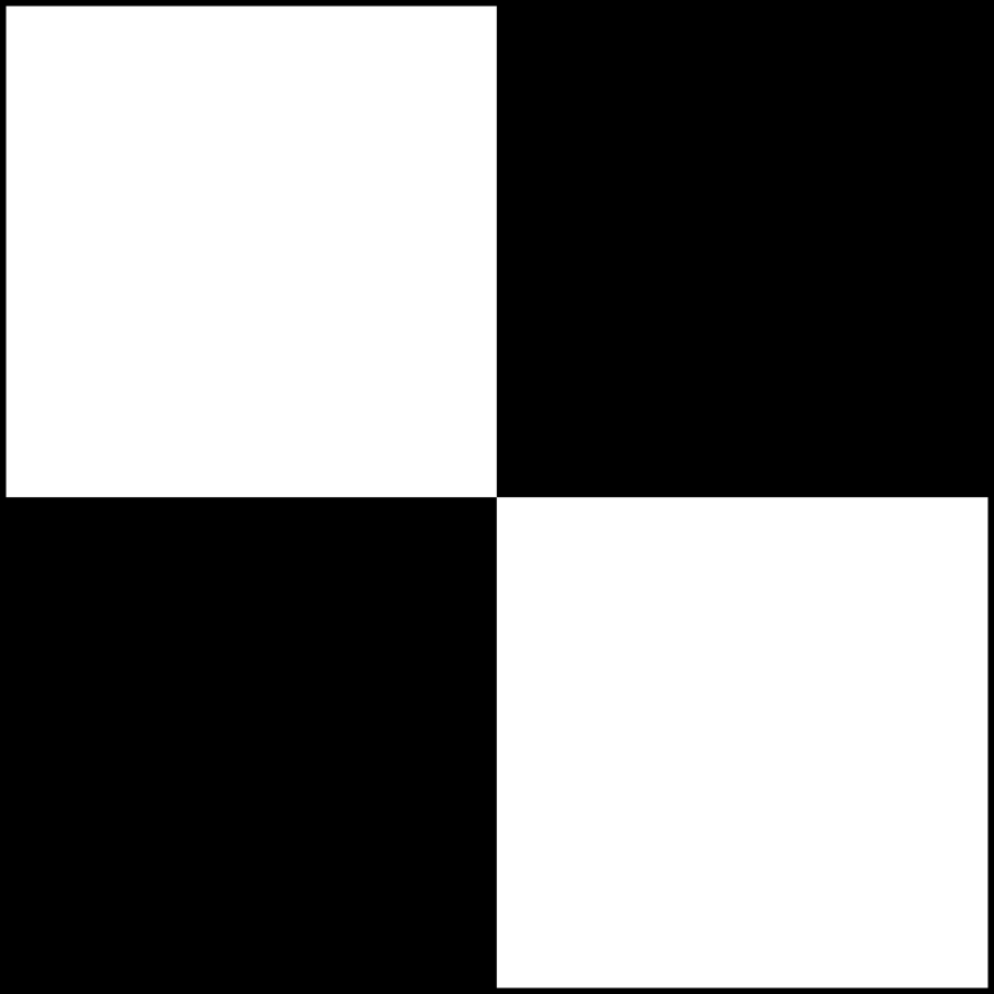
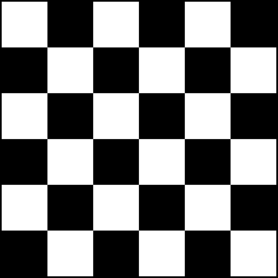
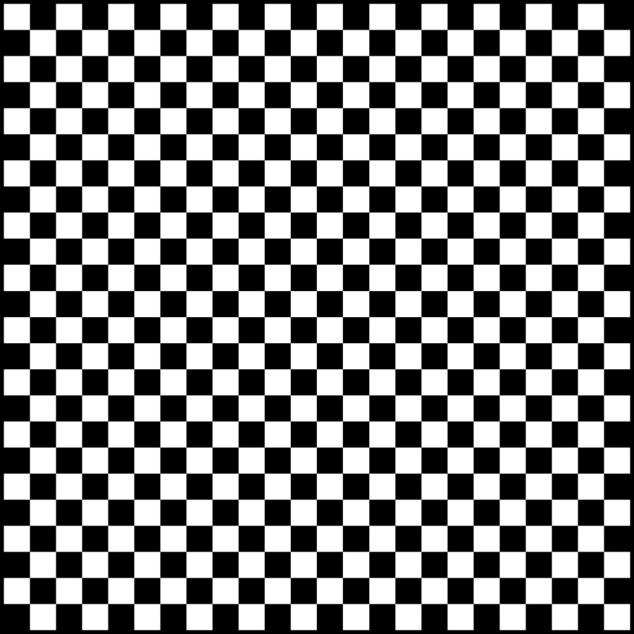
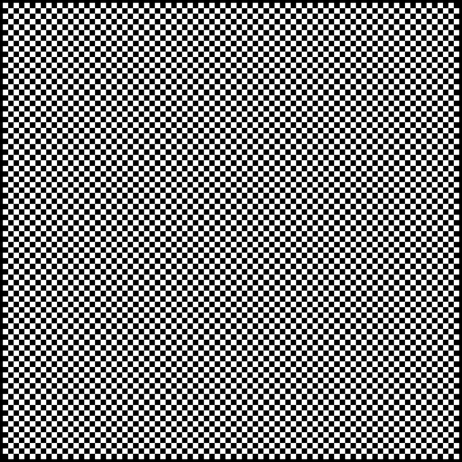
31:224
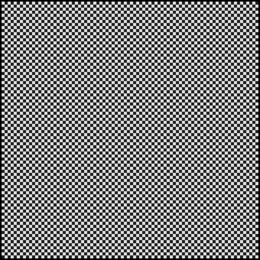
63:192
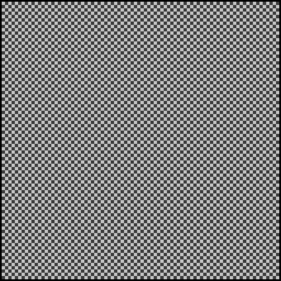
95:160
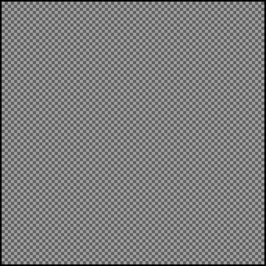
127:128

Figure 1: Model systems of partially miscible blends of 168$\times$168 pixels: checkerboard patterns with varying shades of gray and varying characteristic scales of 84$\times$84, 28$\times$28, 12$\times$12, 7$\times$7, and 2$\times$2 pixels. The intensities of black and white regions are the same in each row and are indicated in the first column.

Figure 2: Inhomogeneity functions for the patterns in Fig. 1 as a function of the resolution scale. The “black” and “white” intensities are (a) 0:255, (b) 31:224, (c) 63:192, (d) 95:160 and (e) 127:128.

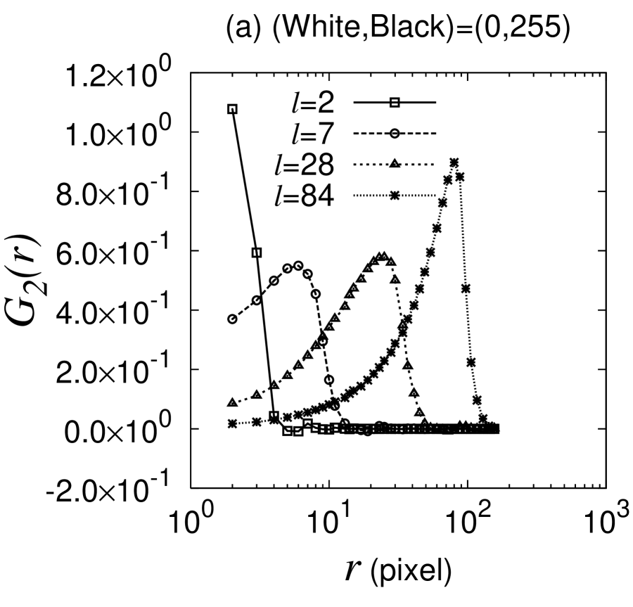
Figure 3: Scale susceptibility to the resolution scale, $G_{2}(r)$, for the systems in Fig. 1 as a function of the resolution scale. The “black” and “white” intensities are (a) 0:255, (b) 31:224, (c) 63:192, (d) 95:160 and (e) 127:128.

III Results and discussion

III.1 Application to particle dispersions

A particle dispersion and a composite material are typical examples of a multi-component system, which consists of small particles and a matrix medium. The physical properties of a dispersion are not solely determined by those of the particles and the matrix medium but also depend on the distribution of the particles. The structure of the particle distribution is controlled by the non-equilibrium processing history, as well as by the thermodynamic stability of the structure. The mixture state of a dispersion should not be characterized solely by the primary particle size but also by multiple scales associated with particle distributions. We apply the moment function method for characterization of different states of synthetic particle dispersions.

Consider monodisperse dispersions with a diameter of the particles $d=10$ pixels that is a natural characteristic scale of the systems. For the sake of simplicity, two-dimensional systems are analyzed, but application to three-dimensional systems is straightforward. Three different dispersions with an area fraction of the particles of 0.1 are depicted in Fig. 4(a)-(c). The particles are randomly distributed in Fig. 4(a), the particles are locally ordered in Fig. 4(b) and several particles aggregate in Fig. 4(c).

(a)

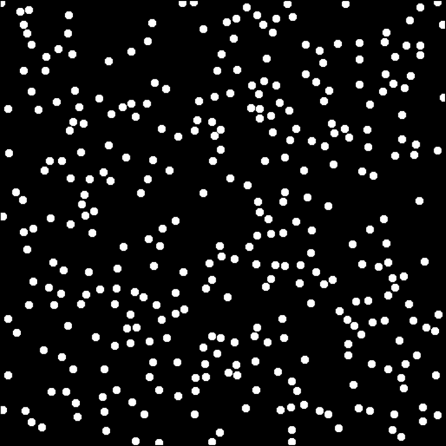
(b)

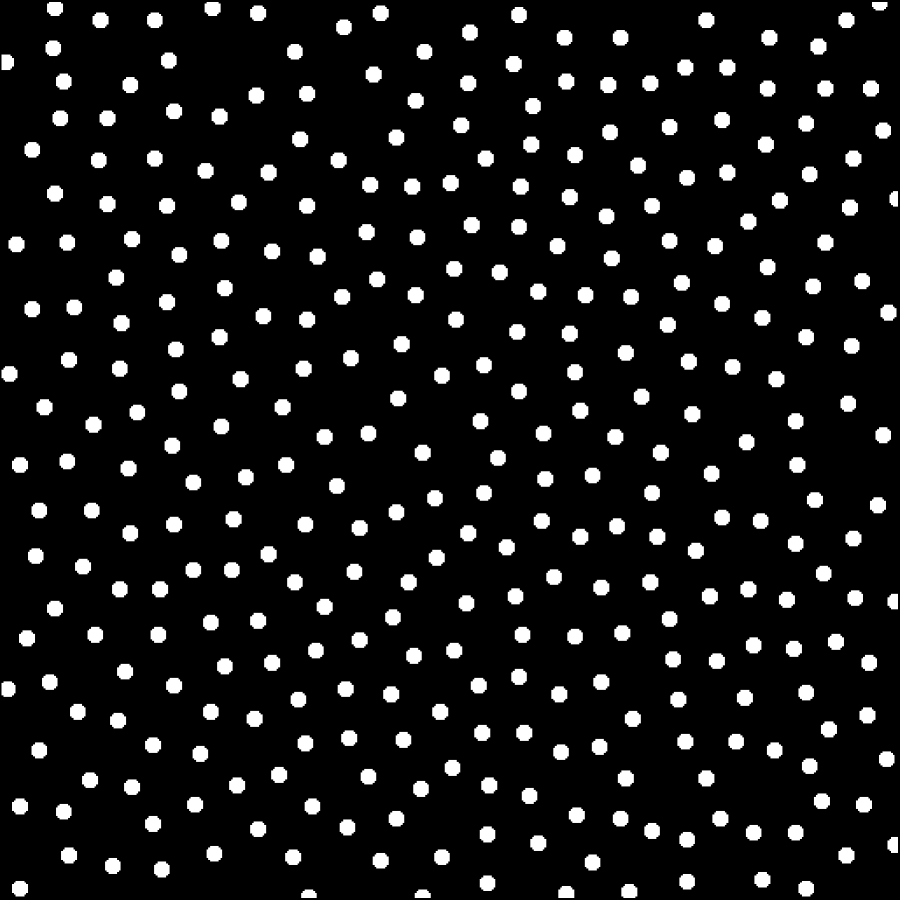
(c)

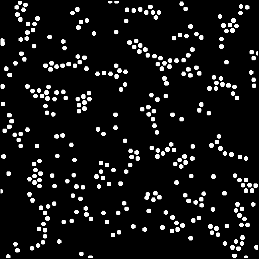
(d)

(e)

(f)

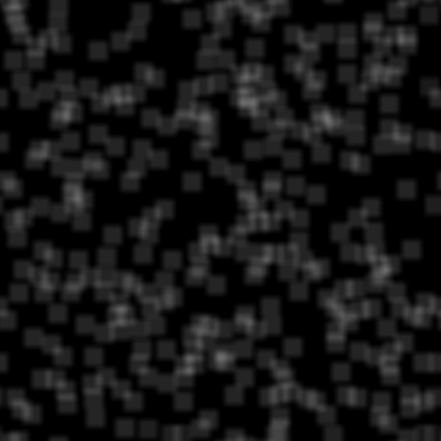
(g)

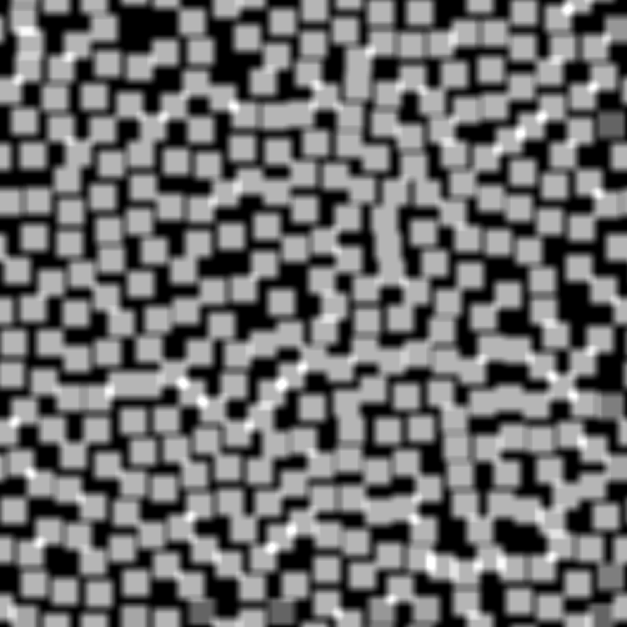
(h)

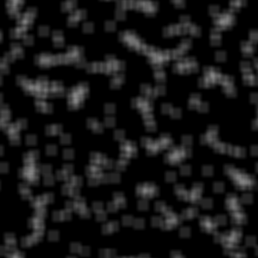
Figure 4: Particle dispersion and their multiple-scale inhomogeneity. Three different particle dispersions of 512$\times$512 pixels: (a) particles are randomly distributed, (b) particles are locally ordered, and (c) particles are aggregated. The area fraction of the systems is 0.1 and the diameter of the particles is $d=10$ pixels. (d) The inhomogeneity functions, $F_{4}(r)$, and the scale susceptibilities, $G_{4}(r)$, for the systems (a)-(c). Coarse-grained fields, $\mu_{22}(\mbox{\boldmath$x$})$, for (f) random dispersion, (g) ordered dispersion and (h) aggregated dispersion.

The inhomogeneity function, $F_{4}(r)$, and the scale susceptibility, $G_{4}(r)$, for the three systems in Figs. 4(a)-(c) are shown in Fig. 4(d) and Fig. 4(e), respectively. In this case, the concentration field of the particles was analyzed, which was unity in the particle domain and zero in the matrix domain. Because the analysis was applied to binarized systems, a single value of $q$ is sufficient. For clarity of presentation, the results of $q=4$ are shown. For the random dispersion in Fig. 4(a), there are no coherence scales other than $d$ because the particles are randomly distributed by construction. The $F_{4}(r)$ and $G_{4}(r)$ for the random dispersion indicate the particle size by the large fluctuation at $r=d$ and the scale of homogeneity for $l_{H}^{\text{random}}\approx 10d$. The ratio $l_{H}^{\text{random}}/d=10$ is relatively large, which explains the inhomogeneity of the particle distribution.

In the system of Fig. 4(b), inter-particle distances between nearest pairs are almost the same, and the particles are locally ordered; therefore we call the system an ordered dispersion for convenience. The average inter-particle distance is $r_{1}\approx 2.7d$, which was measured by the first peak in the correlation function or the pair correlation function. The $r_{1}$ and $d$ are the natural characteristic scales in the ordered dispersion. The large fluctuation at $r=d$ in $F_{4}(r)$ and $G_{4}(r)$ for the ordered dispersion indicates the particle size. At $r>r_{1}$ in $F_{4}(r)$, the fluctuation almost vanishes because the structural fluctuation does not exists at large scale. A close examination of $G_{4}(r)$ reveals a small peak at around $r\approx 4d$, which can be ascribed to the fluctuation in a middle-range scale. The scale of homogeneity is about $l_{H}^{\text{ordered}}\approx 6d$. If the ordered configuration developed globally, $l_{H}^{\text{ordered}}\approx r_{1}$ would be expected because the fluctuation $r>r_{1}$ did not exist. The ordered configuration makes the scale of homogeneity smaller than that of the random dispersion.

In the system of Fig. 4(c), several particles aggregate, and these aggregates are distributed randomly in an aggregated dispersion. One aggregate is composed of 2-20 particles, thus the aggregated dispersion should be characterized by the multiple sizes of the aggregates and the nearest-neighbor distance $r_{1}=1.2d$ in an aggregate besides the particle size $d$. In addition to the large fluctuation at $r=d$ by the particle size, another broad band at $r_{1}<r<10d$ in $G_{4}(r)$ are observed, which corresponds to the multiple sizes of the aggregates. The scale of homogeneity is about $l_{H}^{\text{aggregate}}\approx 10d$, which is similar to that in the random dispersion and much greater than that in the ordered dispersion because of the random distribution of the aggregates. Difference of mixture quality among three dispersions is obvious in the scale susceptibility function, $G_{4}(r)$, in Fig. 4(e). Identification of multiple characteristic scales based on inhomogeneity is essential to quantify mixture quality.

Figures 4(f)-(h) show the coarse-grained fields of the particle dispersions in Figs. 4(a)-(c) with the resolution scale of $r=2.2d$. At this resolution scale, a single particle is hardly discernible. In Fig. 4(b), the $\mu_{22}(\mbox{\boldmath$x$})$ for the ordered dispersion, which has the smallest $l_{H}$, shows the smallest contrast indicating the smallest fluctuation. For the random dispersion, $\mu_{22}(\mbox{\boldmath$x$})$ shows a random structure in the fluctuation (Fig. 4(a)). For the aggregated dispersion, $\mu_{22}(\mbox{\boldmath$x$})$ shows a streak structure and the largest fluctuation among the three systems (Fig. 4(c)).

Coarse-graining is a key concept in simultaneous characterization of various characteristic scales associated with a hierarchical structure and inhomogeneity of distribution. The demonstration with the different dispersions above showed how the scale-dependent moment method works to assess different characteristic scales including the particle size, aggregate sizes, and inter-particle spacing.

IV Concluding remarks

We proposed a method for characterization of hierarchical mixture quality of complex mixtures , which we call the scale-dependent moment function method. In this method, the inhomogeneity of a mixture is defined at different scales. From this scale-dependent inhomogeneity, multiple characteristic scales in mixture quality are identified. In other words, the sizes and distributions of internal structures are simultaneously accounted for in the scale-dependent moment function. Application of this method to dispersions with different structures showed that differences in mixture quality are characterized by multiple length scales and associated inhomogeneity.

The scale-dependent moment method is applicable to two- or three- dimensional concentration fields. The mixture quality characterization based on the scales and inhomogeneity should be effective not only for multi-component complex mixtures with hierarchical internal structures but also for the evolution of the mixing process of both miscible and immiscible mixtures. It is expected that this proposed multiple-scale characterization can provide an insight on the relationship between the distribution of internal structures and the physical properties of mixture materials, but this issue is left for future work.

References

- (1) L. M. Robeson, Polymer blends: a comprehensive review (Hanser Fachbuchverlag, Munich, 2007).
- (2) D. W. Schaefer and R. S. Justice, Macromolecules 40, 8501 (2007).
- (3) R. A. Vaia and J. F. Maguire, Chem. Mater. 19, 2736 (2007).
- (4) D. R. Paul and L. M. Robeson, Polymer 49, 3187 (2008).
- (5) R. F. Gibson, Compos. Struct. 92, 2793 (2010).
- (6) Z. Tadmor and C. G. Gogos, Principles of Polymer Processing, 2nd ed. (Wiley-Interscience, Hoboken, N.J., 2006).
- (7) Food Mixing: Principles and Applications, edited by P. J. Cullen (Wiley-Blackwell, Chichester, U.K., 2009).
- (8) K. Muthukumarappan, in Food Mixing: Principles and Applications, edited by P. J. Cullen (Wiley-Blackwell, Chichester, U.K., 2009), Chap. 2.
- (9) J. M. Ottino and R. Chella, Polym. Eng. Sci. 23, 357 (1983).
- (10) D. Bigio and W. Stry, Polym. Eng. Sci. 30, 153 (1990).
- (11) Z. B. Stone and H. A. Stone, Phys. Fluids 17, 063103 (2005).
- (12) M. Funakoshi, Fluid Dyn. Res. 40, 1 (2008).
- (13) D. Bothe, C. Stemich, and H. Warnecke, Chem. Eng. Sci. 61, 2950 (2006).
- (14) D. Bothe, C. Stemich, and H. Warnecke, Comput. Chem. Eng. 32, 108 (2008).
- (15) Y. Zhu et al., Compos. Struct. 92, 2203 (2010).
- (16) Z. Li et al., Polymer 53, 1571 (2012).
- (17) I. H. Sul, J. R. Youn, and Y. S. Song, Carbon 49, 1473 (2011).
- (18) H. H. Yang, T. H. Wong, and I. Manas-Zloczower, in Mixing and compounding of polymers: Theory and practice, edited by I. Manas-Zloczower and Z. Tadmor (Carl Hanser Verlag, New York, 1994), pp. 189–223.
- (19) H.-H. Yang and I. Manas-Zloczower, in Mixing and Compounding of Polymers: Theory and Practice, 2 har/pas ed., edited by I. Manas-Zloczower (Hanser Gardner Publications, ADDRESS, 2009), Chap. 8, pp. 269–298.
- (20) R. K. Connelly and J. L. Kokini, Journal of Food Engineering 79, 956 (2007).
- (21) Alemaskin, Kirill, Manas-Zloczower, Ica, and Kaufman, Miron, Polym. Eng. Sci. 45, 1011 (2005).
- (22) M. Camesasca and I. Manas-Zloczower, Macromolecular Theory and Simulations 18, 87 (2009).
- (23) P. V. Danckwerts, Appl. Sci. Res. A 3, 279 (1952).
- (24) H. S. Khare and D. L. Burris, Polymer 51, 719 (2010).
- (25) S. Pegel et al., Polymer 50, 2123 (2009).
- (26) G. Mathew, I. Mezic, and L. Petzold, Physica D 211, 23 (2005).
- (27) A. N. Kolmogorov, J. Fluid Mech. 13, 82 (1962).
- (28) A. M. Oboukhov, J. Fluid Mech. 13, 77 (1962).
- (29) B. B. Mandelbrot, The Fractal Geometry of Nature, 1 ed. (W.H. Freeman, New York, 1982).
- (30) H. Fujisaka and Y. Nakayama, Phys. Rev. E 67, 026305 (2003).
- (31) H. Fujisaka and T. Yamada, Prog. Theor. Phys. 77, (1987).