Electric dipole polarizabilities of alkali metal ions from perturbed relativistic coupled-cluster theory

Abstract

We use the perturbed relativistic coupled-cluster theory to compute the static electric dipole polarizabilities of the singly ionized alkali atoms, namely, Na⁺, K⁺, Rb⁺, Cs⁺ and Fr⁺. The computations use the Dirac-Coulomb-Breit Hamiltonian with the no-virual-pair approximation and we also estimate the correction to the static electric dipole polarizability arising from the Breit interaction.

I Introduction

The electric dipole polarizabilities, $\alpha$, of ions are important to determine the optical properties of ionic crystals. In addition, for closed-shell ions like the singly ionized alkali atoms, $\alpha$ is a measure of the core-polarization effects in the neutral species. It is, however, nontrivial to measure $\alpha$ of ions. For the singly charged alkali ions, an indirect method to determine $\alpha$ is through the measurement of the transition energy between the non-penetrating Rydberg states of the neutral species Mayer and Mayer (1933) and it has been used to determine the $\alpha$ of Cs⁺ Ruff et al. (1980); Safinya et al. (1980). In absence of experimental data, there is a need for accurate theoretical calculations. In the case of neutral atoms, accurate values of polarizabilities are essential in studies related to the parity non-conservation in atoms Khriplovich (1991), optical atomic clocks Udem et al. (2002); Diddams et al. (2004) and physics with the condensates of dilute atomic gases Anderson et al. (1995); Bradley et al. (1995); Davis et al. (1995) are of current interest.

Theoretically, methods based on a wide range of atomic many-body theories have been used to calculate $\alpha$. In this regard, the recent review Mitroy et al. (2010) provides description about the various theoretical methods used to calculate $\alpha$. In the present work we use the perturbed relativistic coupled-cluster (PRCC) theory, which was earlier applied the noble gas atoms Chattopadhyay et al. (2012a, b), to compute the $\alpha$ of the singly charged alkali ions. The PRCC theory is an extension of the standard relativistic coupled-cluster (RCC) theory to include an additional perturbation and for this, we introduce a new set of cluster operators. The formulation is, however, general enough to incorporate any perturbation Hamiltonian. It must be emphasized that, compared to other many-body methods, the use of PRCC is an attractive option as it is based on coupled-cluster theory (CCT) Coester (1958); Coester and Kümmel (1960): an all order many-body theory considered to be reliable and powerful. The recent review Bartlett and Musiał (2007) provides an overview of CCT, and variants of CCT developed for structure and properties calculations. The theory has been widely used for atomic Mani et al. (2009); Nataraj et al. (2008); Pal et al. (2007); Gopakumar et al. (2001), molecular Isaev et al. (2004), nuclear Hagen et al. (2008) and condensed matter physics Bishop et al. (2009) calculations. Coming back to the PRCC theory, it is different from the other RCC based theories in a number of ways, but the most important one is the representation of the cluster operators. In the PRCC theory, the cluster operators can be scalar or rank one tensor operators and it is decided based on the nature of the perturbation in the electronic sector. Consequently, the theory is suitable to incorporate multiple perturbations of different ranks in the electronic sector.

One basic advantage of PRCC theory is, it does away with the summation over intermediate states in the first order time-independent perturbation theory. The summation is subsumed in the perturbed cluster amplitudes and this offers significant advantages in computing properties like $\alpha$ which involves summation over a complete set of intermediate states.

The paper is organized as follows. In the Sec. II, for completeness and easy reference we briefly describe the RCC and PRCC theories with the Breit interaction. In Sec. IV we introduce the formal expression of the dipole polarizability and its representation in the PRCC theory. In the subsequent sections we describe the calculational part, and present the results and discussions. We then end with conclusions. All the results presented in this work and related calculations are in atomic units ( $\hbar=m_{e}=e=4\pi\epsilon_{0}=1$). In this system of units the velocity of light is $\alpha^{-1}$, the inverse of fine structure constant. For which we use the value of $\alpha^{-1}=137.035\;999\;074$ Mohr et al. (2012).

II Overview of the coupled-cluster theory

The detailed description of the RCC and PRCC theories are given in our previous works. However, for completeness and easy reference we provide a brief overview in this section.

II.1 RCC theory

The Dirac-Coulomb-Breit Hamiltonian, denoted by $H^{\rm DCB}$, is an appropriate choice to include the relativistic effects in the structure and property calculations of high-$Z$ atoms and ions. There are, however, complications associated with the negative energy continuum states of $H^{\rm DCB}$. These lead to variational collapse and continuum dissolution Brown and Ravenhall (1951). One remedy to avoid these complications is to use the no-virtual pair approximation. In this approximation, for a singly charged ion of $N$ electrons Sucher (1980)

$$H^{\rm DCB} = \Lambda_{++}\sum_{i=1}^{N}\left[c\bm{\alpha}_{i}\cdot\mathbf{p}_{i}+(\beta_{i}-1)c^{2}-V_{N+1}(r_{i})\right]$$ (1)

$$+\sum_{i<j}\left[\frac{1}{r_{ij}}+g^{\rm B}(r_{ij})\right]\Lambda_{++},$$

where $\alpha$ and $\beta$ are the Dirac matrices, $\Lambda_{++}$ is an operator which projects to the positive energy solutions and $V_{N}(r_{i})$ is the electrostatic potential arising from the $Z=(N+1)$ nucleus. Projecting the Hamiltonian with $\Lambda_{++}$ ensures that the effects of the negative energy continuum states are removed from the calculations. The last two terms in $H^{\rm DCB}$, $1/r_{ij}$ and $g^{\rm B}(r_{ij})$, are the Coulomb and Breit interactions, respectively. The later, Breit interaction, represents the transverse photon interaction and is given by

$$g^{\rm B}(r_{12})=-\frac{1}{2r_{12}}\left[\bm{\alpha}_{1}\cdot\bm{\alpha}_{2}+\frac{(\bm{\alpha_{1}}\cdot\mathbf{r}_{12})(\bm{\alpha_{2}}\cdot\mathbf{r}_{12})}{r_{12}^{2}}\right].$$ (2)

The Hamiltonian satisfies the eigen-value equation

$$H^{\rm DCB}|\Psi_{i}\rangle=E_{i}|\Psi_{i}\rangle,$$ (3)

where, $|\Psi_{i}\rangle$ is the exact atomic state. In CCT the exact atomic state is defined as

$$|\Psi_{i}\rangle=e^{T^{(0)}}|\Phi_{i}\rangle,$$ (4)

where $|\Phi_{i}\rangle$ is the reference state wave-function and $T^{(0)}$ is the unperturbed cluster operator, which incorporates the residual Coulomb interaction to all orders. We have introduced the superscript to distinguish it from the second set of cluster operators, the perturbed cluster operators, to be introduced later. In the case of a closed-shell ion, the model space of the ground state consists of a single Slater determinant, $|\Phi_{0}\rangle$, and $T^{(0)}=\sum_{i=1}^{N}T_{i}^{(0)}$, where $i$ is the order of excitation. However, in actual computations, incorporating $T_{i}^{(0)}$ with $i\geqslant 4$ is difficult with the existing computational resources. A simplified, but quite accurate approximation is the coupled-cluster single and double (CCSD) excitation approximation, in which

$$T^{(0)}=T_{1}^{(0)}+T_{2}^{(0)}.$$ (5)

This is an approximation which embodies all the important electron correlation effects, and is a good starting point for structure and properties calculations of closed-shell ions. In the second quantized notations

$$T_{1}^{(0)} = \sum_{a,p}t_{a}^{p}{{a}_{p}^{\dagger}}a_{a},$$ (6a)

$$T_{2}^{(0)} = \frac{1}{2!}\sum_{a,b,p,q}t_{ab}^{pq}{{a}_{p}^{\dagger}}{{a}_{q}^{\dagger}}a_{b}a_{a},$$ (6b)

where $t_{\ldots}^{\ldots}$ are cluster amplitudes, $a_{i}^{\dagger}$ ($a_{i}$) are single particle creation (annihilation) operators and $abc\ldots$ ($pqr\ldots$) represent core (virtual) states. For the present work, the ground state is the required atomic state $|\Psi_{0}\rangle=e^{{T^{(0)}}}|\Phi_{0}\rangle$ and satisfies the eigenvalue equation

$$H^{\rm DCB}e^{{T^{(0)}}}|\Phi_{0}\rangle=E_{0}e^{{T^{(0)}}}|\Phi_{0}\rangle,$$ (7)

where, $E_{0}$ and $|\Phi_{0}\rangle$ are the energy and reference state of the ground state, respectively. Following similar procedure, the CC eigenvalue equation of the one-valence Mani and Angom (2010) and two-valence Mani and Angom (2011) systems may be defined.

II.2 PRCC Theory

In the PRCC theory we introduce a new set of cluster operators, $\mathbf{T^{(1)}}$, to incorporate an interaction Hamiltonian, $H_{\rm int}$, perturbatively. For general representation, we consider $\mathbf{T^{(1)}}$ as tensor operators of arbitrary rank and depends on the multipole structure of $H_{\rm int}$. The new cluster operators follow the selection rules associated with $H_{\rm int}$ and the modified ground state eigenvalue equation, after including the perturbation, is

$$(H^{\rm DCB}+\lambda H_{\rm int})|\tilde{\Psi}_{0}\rangle=\tilde{E}_{0}|\tilde{\Psi}_{0}\rangle,$$ (8)

where $\lambda$ is the perturbation parameter, $|\tilde{\Psi}_{0}\rangle$ is the perturbed ground state and $\tilde{E}_{0}$ is the corresponding eigen energy. To calculate the electric dipole polarizability, $\alpha$, consider the perturbation as the interaction with an electrostatic field $\mathbf{E}$. The interaction Hamiltonian is then $H_{\rm int}=-\sum_{i}\mathbf{r}_{i}\cdot\mathbf{E}=\mathbf{D}\cdot\mathbf{E}$, where $\mathbf{D}$ is the many electron electric dipole operator. Here, $H_{\rm int}$ is odd in parity and to be more precise, $\mathbf{D}$, the operator in the electronic space is odd in parity and a rank one operator. Hence, the cluster opertors $\mathbf{T^{(1)}}$ are also rank one tensor operators and odd in parity, meaning, they connect states of different parities. Further more, the first energy correction $\langle\Psi_{0}|H_{\rm int}|\Psi_{o}\rangle=0$ and therefore, $\tilde{E}_{0}=E_{0}$. We can then write, using PRCC theory, the perturbed ground state as

$$|\tilde{\Psi}_{0}\rangle=e^{T^{(0)}+\lambda\mathbf{T}^{(1)}\cdot\mathbf{E}}|\Phi_{0}\rangle=e^{T^{(0)}}\left[1+\lambda\mathbf{T^{(1)}\cdot\mathbf{E}}\right]|\Phi_{0}\rangle,$$ (9)

where, we have introduced the scalar product between $\mathbf{T}^{(1)}$ and $\mathbf{E}$ for a consistent representation of the states and operators. The advatage of introducing $\mathbf{T^{(1)}}$ and using $|\tilde{\Psi}_{0}\rangle$ is, it allows a systematic consolidation of the correlation effects arising from multiple perturbations.

Based on the analysis of the low-order many-body perturbation theory diagrams, the single and double excitation operators of PRCC theory are represented as

$$\mathbf{T}_{1}^{(1)} = \sum_{a,p}\tau_{a}^{p}\mathbf{C}_{1}(\hat{r})a_{p}^{\dagger}a_{a},$$ (10a)

$$\mathbf{T}_{2}^{(1)} = \sum_{a,b,p,q}\sum_{l,k}\tau_{ab}^{pq}(l,k)\{\mathbf{C}_{l}(\hat{r}_{1})\mathbf{C}_{k}(\hat{r}_{2})\}^{1}a_{p}^{\dagger}a_{q}^{\dagger}a_{b}a_{a}.\;\;\;\;\;\;\;\;$$ (10b)

where $\tau_{\ldots}^{\ldots}$ are the cluster amplitudes and $\mathbf{C}_{i}(\hat{r})$ are $\mathbf{C}$-tensors of rank $i$. To represent $\mathbf{T}_{1}^{(1)}$, a rank one operator, we have used the $\mathbf{C}$-tensor of similar rank $\mathbf{C}_{1}(\hat{r})$. And, the key difference of $\mathbf{T}_{1}^{(1)}$ from $T_{1}^{(0)}$ is $l_{a}+l_{p}$ must be odd, in other words $(-1)^{l_{a}+l_{p}}=-1$, where, $l_{a}$ ($l_{p}$) is the orbital angular momentum of the core (virtual) state $a$ ($p$). Coming to $\mathbf{T}_{2}^{(1)}$, to represent it two $\mathbf{C}$-tensor operators of rank $l$ and $k$ are coupled to a rank one tensor operator. In terms of selection rules, the angular momenta of the orbitals and multipoles in $\mathbf{T}_{2}^{(1)}$ must satisfy the triangular conditions $|j_{a}-j_{p}|\leqslant l\leqslant(j_{a}+j_{p})$, $|j_{b}-j_{q}|\leqslant k\leqslant(j_{b}+j_{q})$ and $|l-k|\leqslant 1\leqslant(l+k)$. The other selection rule follows from the parity of $H_{\rm int}$, the orbital angular momenta must satisfy the condition $(-1)^{(l_{a}+l_{p})}=-(-1)^{(l_{b}+l_{q})}$.

II.3 PRCC equations

The ground state eigenvalue equation, in terms of the PRCC state, is

$$H^{\rm DCB}e^{\left[T^{(0)}+\lambda\mathbf{T}^{(1)}\cdot\mathbf{E}\right]}|\Phi_{0}\rangle=E_{0}e^{\left[T^{(0)}+\lambda\mathbf{T}^{(1)}\cdot\mathbf{E}\right]}|\Phi_{0}\rangle.$$ (11)

In the CCSD approximation we define the perturbed cluster operator $\mathbf{T}^{(1)}$ as

$$\mathbf{T}^{(1)}=\mathbf{T}_{1}^{(1)}+\mathbf{T}_{2}^{(1)}.$$ (12)

Using this, the PRCC equations are derived from Eq. (11). The derivation involves several operator contractions and these are more transparent with the normal ordered Hamiltonian $H_{\rm N}^{\rm DCB}=H^{\rm DCB}-\langle\Phi_{i}|H^{\rm DCB}|\Phi_{i}\rangle$. The eigenvalue equation then assumes the form

$$\left[H^{\rm DCB}_{N}+\lambda H_{\rm int}\right]|\tilde{\Psi}_{0}\rangle=\left[E_{0}-\langle\Phi_{0}|H^{\rm DCB}|\Phi_{0}\rangle\right]|\tilde{\Psi}_{0}\rangle.$$ (13)

A more convenient form of the equation is

$$\left(H^{\rm DCB}_{\rm N}+\lambda H_{\rm int}\right)|\tilde{\Psi}_{0}\rangle=\Delta E_{0}|\tilde{\Psi}_{0}\rangle,$$ (14)

where, $\Delta E_{0}=E_{0}-\langle\Phi_{0}|H^{\rm DCB}|\Phi_{0}\rangle$ is the ground state correlation energy. Following the definition in Eq. (9), the PRCC eigen-value equation is

$$\left(H^{\rm DCB}_{\rm N}+\lambda H_{\rm int}\right)e^{T^{(0)}+\lambda\mathbf{T}^{(1)}\cdot\mathbf{E}}|\Phi_{0}\rangle=\Delta E_{0}e^{T^{(0)}+\lambda\mathbf{T}^{(1)}\cdot\mathbf{E}}|\Phi_{0}\rangle.$$ (15)

Applying $e^{-T^{(0)}}$ from the left, we get

$$\left[\bar{H}^{\rm DCB}_{\rm N}+\lambda\bar{H}_{\rm int}\right]e^{\lambda\mathbf{T}^{(1)\cdot\mathbf{E}}}|\Phi_{0}\rangle=\Delta E_{0}e^{\lambda\mathbf{T}^{(1)}\cdot\mathbf{E}}|\Phi_{0}\rangle,$$ (16)

where $\bar{H}^{\rm DCB}=e^{-T^{(0)}}H^{\rm DCB}e^{T^{(0)}}$ is the similarity transformed Hamiltonian. Multiplying Eq. (16) from left by $e^{-\lambda\mathbf{T}^{(1)}}$ and considering the terms linear in $\lambda$, we get the PRCC equation

$$\left[\bar{H}^{\rm DC}_{\rm N},\mathbf{T}^{(1)}\right]\cdot\mathbf{E}+\bar{H}_{\rm int}|\Phi_{0}\rangle=0.$$ (17)

Here, the similarity transformed interaction Hamiltonian $\bar{H}_{\rm int}$ terminates at second order as $H_{\rm int}$ is a one-body interaction Hamiltonian. Expanding $\bar{H}_{\rm int}$ and dropping $\mathbf{E}$ for simplicity, the PRCC equation assumes the form

$$\left[\bar{H}_{\rm N}^{\rm DCB},\mathbf{T}^{(1)}\right]|\Phi_{0}\rangle = \bigg{(}\mathbf{D}+\left[\mathbf{D},T^{(0)}\right]$$ (18)

$$+\frac{1}{2}\left[\left[\mathbf{D},T^{(0)}\right],T^{(0)}\right]\bigg{)}|\Phi_{0}\rangle.\;\;\;$$

The equations of $\mathbf{T}_{1}^{(1)}$ are obtained after projecting the equation on singly excited states $\langle\Phi_{a}^{p}|$. These excitation states, however, must be opposite in parity to $|\Phi_{0}\rangle$. The $\mathbf{T}_{2}^{(1)}$ equations are obtain in a similar way after projecting on the doubly excited states $\langle\Phi_{ab}^{pq}|$. The equations form a set of coupled nonlinear algebraic equations. The equations and a description of the different terms along with diagrammatic analysis are given in our previous works Chattopadhyay et al. (2012a, b). An approximation which incorporates all the important many-body effects like core-polarization is the linearized PRCC (LPRCC). In this approximation, only the terms linear in $T^{(0)}$, equivalent to retaining only $\{\mathchoice{\vbox{\hbox to0.0pt{\kern 0.0pt\kern 4.56248pt\hbox{\vrule width=0.50003pt,height=0.0pt,depth=2.15277pt\vrule width=12.3788pt,height=0.0pt,depth=0.50003pt\vrule width=0.50003pt,height=0.0pt,depth=2.15277pt}\hss}\vskip 2.15277pt\vskip 6.83331pt}}{\vbox{\hbox to0.0pt{\kern 0.0pt\kern 4.56248pt\hbox{\vrule width=0.50003pt,height=0.0pt,depth=2.15277pt\vrule width=12.3788pt,height=0.0pt,depth=0.50003pt\vrule width=0.50003pt,height=0.0pt,depth=2.15277pt}\hss}\vskip 2.15277pt\vskip 6.83331pt}}{\vbox{\hbox to0.0pt{\kern 0.0pt\kern 3.19374pt\hbox{\vrule width=0.50003pt,height=0.0pt,depth=2.15277pt\vrule width=8.72516pt,height=0.0pt,depth=0.50003pt\vrule width=0.50003pt,height=0.0pt,depth=2.15277pt}\hss}\vskip 2.15277pt\vskip 4.78333pt}}{\vbox{\hbox to0.0pt{\kern 0.0pt\kern 2.28123pt\hbox{\vrule width=0.50003pt,height=0.0pt,depth=2.15277pt\vrule width=7.0894pt,height=0.0pt,depth=0.50003pt\vrule width=0.50003pt,height=0.0pt,depth=2.15277pt}\hss}\vskip 2.15277pt\vskip 3.41666pt}}H_{\rm N}T^{(1)}\}$ and $\{\mathchoice{\vbox{\hbox to0.0pt{\kern 0.0pt\kern 1.95833pt\hbox{\vrule width=0.50003pt,height=0.0pt,depth=2.15277pt\vrule width=7.50394pt,height=0.0pt,depth=0.50003pt\vrule width=0.50003pt,height=0.0pt,depth=2.15277pt}\hss}\vskip 2.15277pt\vskip 4.30554pt}}{\vbox{\hbox to0.0pt{\kern 0.0pt\kern 1.95833pt\hbox{\vrule width=0.50003pt,height=0.0pt,depth=2.15277pt\vrule width=7.50394pt,height=0.0pt,depth=0.50003pt\vrule width=0.50003pt,height=0.0pt,depth=2.15277pt}\hss}\vskip 2.15277pt\vskip 4.30554pt}}{\vbox{\hbox to0.0pt{\kern 0.0pt\kern 1.37083pt\hbox{\vrule width=0.50003pt,height=0.0pt,depth=2.15277pt\vrule width=5.2803pt,height=0.0pt,depth=0.50003pt\vrule width=0.50003pt,height=0.0pt,depth=2.15277pt}\hss}\vskip 2.15277pt\vskip 3.01389pt}}{\vbox{\hbox to0.0pt{\kern 0.0pt\kern 0.97916pt\hbox{\vrule width=0.50003pt,height=0.0pt,depth=2.15277pt\vrule width=4.16537pt,height=0.0pt,depth=0.50003pt\vrule width=0.50003pt,height=0.0pt,depth=2.15277pt}\hss}\vskip 2.15277pt\vskip 2.15277pt}}\mathbf{r}_{i}T^{(0)}\}$ in the PRCC equations.

Figure 1: Diagrams of the $\alpha$ in the PRCC theory. The single excitation operators with a wavy line represent $\mathbf{T}^{(1)}_{1}$. Similarly, the double excitation diagrams with an extra vertical line represent $\mathbf{T}^{(1)}_{2}$.

III Dipole Polarizability

In the PRCC theory we can write the $\alpha$ of the ground state of a closed-shell atom as Chattopadhyay et al. (2012a, b)

$$\alpha=-\frac{\langle\Phi_{0}|\mathbf{T}^{(1)\dagger}\bar{\mathbf{D}}+\bar{\mathbf{D}}\mathbf{T}^{(1)}|\Phi_{0}\rangle}{\langle\Psi_{0}|\Psi_{0}\rangle},$$ (19)

where, $\bar{\mathbf{D}}=e^{{T}^{(0)\dagger}}\mathbf{D}e^{T^{(0)}}$, represents the unitary transformed electric dipole operator. Retaining only the dominant terms, we obtain

$$\alpha = -\frac{1}{\cal N}\langle\Phi_{0}|\mathbf{T}_{1}^{(1)\dagger}\mathbf{D}+\mathbf{D}\mathbf{T}_{1}^{(1)}+\mathbf{T}_{1}^{(1)\dagger}\mathbf{D}T_{2}^{(0)}+T_{2}^{(0)\dagger}\mathbf{D}\mathbf{T}_{1}^{(1)}$$ (20)

$$+\mathbf{T}_{1}^{(1)\dagger}\mathbf{D}T_{1}^{(0)}+T_{1}^{(0)\dagger}\mathbf{D}\mathbf{T}_{1}^{(1)}+\mathbf{T}_{2}^{(1)\dagger}\mathbf{D}T_{1}^{(0)}$$

$$+T_{1}^{(0)\dagger}\mathbf{D}\mathbf{T}_{2}^{(1)}+\mathbf{T}_{2}^{(1)\dagger}\mathbf{D}T_{2}^{(0)}+T_{2}^{(0)\dagger}\mathbf{D}\mathbf{T}_{2}^{(1)}|\Phi_{0}\rangle,$$

where ${\cal N}=\langle\Phi_{0}|\exp[T^{(0)\dagger}]\exp[T^{(0)}]|\Phi_{0}\rangle$ is the normalization factor, which involves a non-terminating series of contractions between ${T^{(0)}}^{\dagger}$ and $T^{(0)}$. However, in the present work we use ${\cal N}\approx\langle\Phi_{0}|1+T_{1}^{(0)\dagger}T_{1}^{(0)}+T_{2}^{(0)\dagger}T_{2}^{(0)}|\Phi_{0}\rangle$. An evident advantage of computing $\alpha$ with PRCC theory is the absence of summation over the intermediate states $|\Psi_{I}\rangle$. The summation is subsumed in the evaluation of $\mathbf{T}^{(1)}$ in a natural way and eliminates the need for a complete set of intermediate states.

For further analysis and evaluation of the different terms in Eq. (20), we use many-body diagrams or Goldstone diagrams. To evaluate the diagrams we follow the notations and conventions given in ref. Lindgren and Morrison (1986). However, there is an additional feature in the diagrams of $\alpha$, we employ a wavy interaction line to represent the diagrams of $\mathbf{T}^{(1)}_{1}$, so that it is different from the diagrams of $T_{1}^{(0)}$. Similarly, to represent $\mathbf{T}^{(1)}_{2}$ we introduce a vertical line to the interaction line. After due consideration of the equivalent diagrams, the terms in Eq. (20) correspond to 22 unique Goldstone diagrams and these are shown in Fig. 1. The equivalent algebraic expression is

$$\alpha = \sum_{ap}\left({\tau_{a}^{p}}^{*}d_{ap}+d_{ap}^{*}\tau_{a}^{p}\right)+\sum_{abpq}\left[({\tau_{a}^{p}}^{*}d_{bq}^{*}+{\tau_{a}^{q}}^{*}d_{bp}^{*})t_{ab}^{pq}\right.$$ (21)

$$\left.+\tilde{t}_{ab}^{pq*}d_{ap}\tau_{b}^{q}\right]+\sum_{apq}({t_{a}^{q}}^{*}d_{pq}\tau_{a}^{p}+{\tau_{a}^{q}}^{*}d_{pq}t_{a}^{p})$$

$$-\sum_{abp}({t_{b}^{p}}^{*}d_{ab}\tau_{a}^{p}+{\tau_{b}^{p}}^{*}d_{ab}t_{a}^{p})+\sum_{abpq}(\tilde{\tau}_{ab}^{pq*}d_{bq}t_{b}^{q}$$

$$+d_{bq}^{*}t_{b}^{q*}\tilde{\tau}_{ab}^{pq})+\sum_{abpqr}(\tilde{\tau}_{ab}^{rq*}d_{pr}t_{ab}^{pq}+\tilde{t}_{ab}^{rq*}d_{pr}\tau_{ab}^{pq})$$

$$+\sum_{abcpq}(\tilde{\tau}_{cb}^{pq*}d_{ca}t_{ab}^{pq}+\tilde{t}_{cb}^{pq*}d_{ca}\tau_{ab}^{pq}),$$

where $d_{ab}=\langle a|d|b\rangle$, and $\tilde{\tau}_{ab}^{pq}=\tau_{ab}^{pq}-\tau_{ab}^{qp}$ and $\tilde{t}_{ab}^{pq}=t_{ab}^{pq}-t_{ab}^{qp}$ are the antysymmetrized cluster amplitudes.

In the figure, the first two diagrams, Fig. 1(a) and 1(b), are the most important ones. These represent $\mathbf{T}_{1}^{(1)\dagger}\mathbf{D}$ and $\mathbf{D}\mathbf{T}_{1}^{(1)}$, respectively, and subsume DF and the effects of random phase approximation (RPA). The next two diagrams in the figure, Fig.1(c) and Fig.1(d), arise from the term $\mathbf{T}_{1}^{(1)\dagger}\mathbf{D}T_{2}^{(0)}$. Similarly, the diagrams in Fig.1(e-f) correspond to the hermitian conjugate, $T_{2}^{(0)\dagger}\mathbf{D}\mathbf{T}_{1}^{(1)}$. These are the two leading order terms among the second order contributions, in terms of the cluster amplitudes, to $\alpha$. The reason is, both the terms consist of dominant RCC and PRCC amplitudes, $T_{2}^{(0)}$ and $\mathbf{T}_{1}^{(1)}$, respectively.

Among the second order contributions, the next to leading order terms are $\mathbf{T}_{2}^{(1)\dagger}\mathbf{D}T_{2}^{(0)}$ and $T_{2}^{(0)\dagger}\mathbf{D}\mathbf{T}_{2}^{(1)}$. Each of these terms generate four diagrams, which are given in Fig.1(o-r) and Fig.1(s-v) and these correspond to $\mathbf{T}_{2}^{(1)\dagger}\mathbf{D}T_{2}^{(0)}$ and $T_{2}^{(0)\dagger}\mathbf{D}\mathbf{T}_{2}^{(1)}$, respectively. The remaining second order terms, $\mathbf{T}_{1}^{(1)\dagger}\mathbf{D}T_{1}^{(0)}$, $\mathbf{T}_{2}^{(1)\dagger}\mathbf{D}T_{1}^{(0)}$ and their hermitian conjugates, have marginal contributions to $\alpha$. However, for completeness, these are included in the computations.

Table 1: The $\alpha_{0}$ and $\beta$ parameters of the even tempered GTO basis used in the present calculations.

Atom	$s$		$p$		$d$
	$\alpha_{0}$	$\beta$	$\alpha_{0}$	$\beta$	$\alpha_{0}$	$\beta$
$\rm{Na}^{+}$	0.0025	2.210	0.00955	2.125	0.00700	2.750
$\rm{K}^{+}$	0.0055	2.250	0.00995	2.155	0.00690	2.550
$\rm{Rb}^{+}$	0.0052	2.300	0.00855	2.205	0.00750	2.145
$\rm{Cs}^{+}$	0.0097	2.050	0.00975	2.005	0.00995	1.705
$\rm{Fr}^{+}$	0.0068	2.110	0.00645	2.050	0.00985	1.915

IV Calculational details

IV.1 Basis set and nuclear density

The first step of our computations, which is also true of any atomic and molecular computations, is to generate an spin-orbital basis set. For the present work, the basis set is even-tempered gaussian type orbitals (GTOs) Mohanty and Clementi (1990) generated with the Dirac-Hartree-Fock Hamiltonian. This means, the radial part of the spin-orbitals are linear combinations of the Gaussian type functions. The Gaussian type functions which constitutes the large components are of the form

$$g_{\kappa p}^{L}(r)=C^{L}_{\kappa i}r^{n_{\kappa}}e^{-\alpha_{p}r^{2}},$$ (22)

where $p=0,1\ldots m$ is the GTO index and $m$ is the number of gaussian type functions. The exponent $\alpha_{p}=\alpha_{0}\beta^{p-1}$, where $\alpha_{0}$ and $\beta$ are two independent paramters. Similarly, the small components of the spin-orbitals are linear combination of $g_{\kappa p}^{S}(r)$, which are generated from $g_{\kappa p}^{L}(r)$ through the kinetic balance condition Stanton and Havriliak (1984). The GTOs are calculated on a grid Chaudhuri et al. (1999) with optimized values of $\alpha_{0}$ and $\beta$. The optimization is done for individual atoms to match the spin-orbital energies and self consistent field (SCF) energy of GRASP92 Parpia et al. (1996). For the current work, the optimized $\alpha_{0}$ and $\beta$ are listed in Table. 1. For comparison, the spin-orbital energies of Cs⁺ obtained from the GTO and GRASP92 are listed in Table 2. In the table, the deviation of the GTO results from the GRASP92 is $\sim 10^{-3}$, which is quite small. We obtain similar level of deviations for the other ions as well.

Table 2: Core orbital energies of $\rm{Cs}^{+}$ in atomic units.

Orbital	DC	GRASP92 Parpia et al. (1996)
$1s_{1/2}$	$-1330.1173$	$-1330.1129$
$2s_{1/2}$	$-212.5643$	$-212.5673$
$2p_{1/2}$	$-199.4294$	$-199.4288$
$2p_{3/2}$	$-186.4366$	$-186.4358$
$3s_{1/2}$	$-45.9697$	$-45.9695$
$3p_{1/2}$	$-40.4483$	$-40.4455$
$3p_{3/2}$	$-37.8943$	$-37.8917$
$3d_{3/2}$	$-28.3096$	$-28.3030$
$3d_{5/2}$	$-27.7752$	$-27.7682$
$4s_{1/2}$	$-9.5128$	$-9.5106$
$4p_{1/2}$	$-7.4463$	$-7.4437$
$4p_{3/2}$	$-6.9209$	$-6.9188$
$4d_{3/2}$	$-3.4856$	$-3.4921$
$4d_{5/2}$	$-3.3969$	$-3.4038$
$5s_{1/2}$	$-1.4898$	$-1.4933$
$5p_{1/2}$	$-0.9079$	$-0.9139$
$5p_{3/2}$	$-0.8403$	$-0.8459$

The next step, related to spin-orbial basis set, is the choice of an ideal basis set size. For this, we examine the convergence of $\alpha$ using the LPRCC theory. We calculate $\alpha$ starting with a basis set of 50 GTOs and increase the basis set size in steps through a series of calculations. The results of the such a series of calculations are listed in Table. 3, it shows the convergence of $\alpha$ of Cs⁺ as a function of basis set size.

In the present work we have considered finite size Fermi density distribution of the nucleus

$$\rho_{\rm nuc}(r)=\frac{\rho_{0}}{1+e^{(r-c)/a}},$$ (23)

where, $a=t4\ln(3)$. The parameter $c$ is the half charge radius so that $\rho_{\rm nuc}(c)={\rho_{0}}/{2}$ and $t$ is the skin thickness. Coming to the PRCC equations, these are solved iteratively using Jacobi method, we have chosen this method as it is parallelizable. The method, however, is slow to converge. So, to accelerate the convergence we use direct inversion in the iterated subspace (DIIS)Pulay (1980).

Table 3: Convergence pattern of $\alpha$ ($\rm{Cs}^{+}$) as a function of the basis set size.

No. of orbitals	Basis size	$\alpha$
103	$(15s,13p,13d,9f,9g)$	14.9480
117	$(17s,15p,15d,11f,9g)$	14.9235
131	$(19s,17p,17d,11f,11g)$	14.9124
143	$(23s,19p,19d,13f,11g)$	14.9086
159	$(23s,21p,21d,13f,13g)$	14.9077
177	$(25s,23p,23d,15f,15g)$	14.9077

IV.2 Intermediate Diagrams

The PRCC diagrams corresponding to the nonlinear terms are numerous and topologically complex. Further more, in these diagrams, the number of the spin-orbitals involved is large and in general, the diagrams with the largest number of spin-orbitals are associated with the terms $H_{N}T_{2}^{(0)}T_{2}^{(0)}$, $H_{N}T_{1}^{(0)}T_{1}^{(0)}T_{2}^{(0)}$ and $H_{N}T_{1}^{(0)}T_{1}^{(0)}T_{1}^{(0)}T_{1}^{(0)}$. All of these terms have a common feature: the presence of the Coulomb integral $\langle ab|1/r_{12}|pq\rangle$. Returning to the number of spin-orbitals, the $T_{2}^{(0)}$ diagrams arising from any of the three terms mentioned earlier consist of four core and virtual spin-orbitals each. Accordingly, the number of times a diagram is evaluated, $N_{d}$, scales as $n_{o}^{4}n_{v}^{4}$ and sets the computational requirements. Here, $n_{o}$ and $n_{v}$ are the number of core and virtual spin-orbitals, respectively. In the present work, $n_{o}\sim 10$ and $n_{v}\sim 100$ for lighter atoms and moderate sized basis sets, even then $N_{d}\sim 10^{12}$. This is a large number and puts a huge constraint on the computational resources.

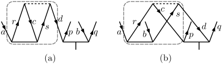
Figure 2: Example diagrams of $H_{N}T_{2}^{(0)}T_{2}^{(0)}$ which contribute to the $\mathbf{T}_{2}^{(1)}$ equations. The portion of the diagrams within the rectangles with rounded corners are examples of the one body (a) and two-body (b) intermediate diagrams.

To mitigate the computational constraints arising from the $n_{o}^{4}n_{v}^{4}$ scaling, we separate the diagrams into two parts. One of the parts scales at the most $n_{o}^{2}n_{v}^{4}$ and the total diagram is equivalent to the product of the parts. The part of the diagram, which is calculated first is referred to as the intermediate diagram. During computations, all the intermediate diagrams are calculated first and stored. Later, these are used to combine with the remaining part of the RCC diagram and the total diagram is calculated. The scaling is still $n_{o}^{2}n_{v}^{4}$ and compared to the $n_{o}^{4}n_{v}^{4}$ scalling, this improves the performance by several orders of magnitudes.

To examine in more detail, consider the term $H_{N}T_{2}^{(0)}\mathbf{T}_{2}^{(1)}$, the algebraic expression for one of the terms contributing to the $\mathbf{T}_{2}^{(0)}$ is

$$\left(\tau_{ab}^{pq}\right)_{\rm 2a}a_{p}^{\dagger}a_{q}^{\dagger}a_{b}a_{a}=\sum_{rcsd}t_{ac}^{rs}v_{rs}^{cd}\tau_{db}^{pq}a_{p}^{\dagger}a_{q}^{\dagger}a_{b}a_{a},$$ (24)

and it is diagrammatically equivalent to Fig. 2(a). However, while evaluating the diagram, the part within the dashed round rectangle or the intermediate diagram can be separated and computed first. The Eq. (24) can then be written as

$$\left(\tau_{ab}^{pq}\right)_{\rm 2a}a_{p}^{\dagger}a_{q}^{\dagger}a_{b}a_{a}=\sum_{d}\left(\eta_{a}^{d}a_{d}^{\dagger}a_{a}\right)\Big{(}\tau_{db}^{pq}a_{p}^{\dagger}a_{q}^{\dagger}a_{b}a_{d}\Big{)},$$ (25)

where $\eta_{a}^{d}=\sum_{rcs}t_{ac}^{rs}v_{rs}^{cd}$ is the amplitude of the effective one-body operator corresponding to the intermediate diagram. It scales as $n_{o}^{3}n_{v}^{2}$ and when contracted with $\mathbf{T}_{2}^{(1)}$, the computation still cales as $n_{o}^{3}n_{v}^{2}$. This is much less than the $n_{o}^{4}n_{v}^{4}$ scaling. Consider another term

$$\left(\tau_{ab}^{pq}\right)_{\rm 2b}a_{p}^{\dagger}a_{q}^{\dagger}a_{b}a_{a}=\sum_{rcsd}t_{ab}^{rs}v_{rs}^{cd}\tau_{cd}^{pq}a_{p}^{\dagger}a_{q}^{\dagger}a_{b}a_{a},$$ (26)

and it is diagrammatically equivalent to Fig. 2(b). Like in the previous case, the intermediate diagram ( part within the dashed round-rectangle ) can be calculated first and the equation can rewritten as

$$\left(\tau_{ab}^{pq}\right)_{\rm 2b}a_{p}^{\dagger}a_{q}^{\dagger}a_{b}a_{a}=\sum_{cd}\left(\eta_{ab}^{cd}a_{c}^{\dagger}a_{d}^{\dagger}a_{b}a_{a}\right)\Big{(}\tau_{cd}^{pq}a_{p}^{\dagger}a_{q}^{\dagger}a_{d}a_{c}\Big{)}.$$ (27)

Here, the intermediate diagram corresponds to a two-body effective operator with amplitude $\eta_{ab}^{cd}=\sum_{rs}t_{ab}^{rs}v_{rs}^{cd}$ and scales as $n_{o}^{4}n_{v}^{2}$. The scaling remains the same when the total diagram is evaluated. Extending the method to other diagrams, depending on the topology, there are other forms of one-body and two-body intermediate diagrams.

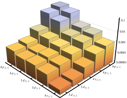
Figure 3: Contributions to the next to leading order terms $\mathbf{T}_{1}{{}^{(1)\dagger}}\mathbf{D}T_{2}^{(0)}$ + h.c. in terms of the pairs of core spin-orbitals.

V Results and Discussions

To compute $\alpha$ using PRCC theory, as described earlier, we consider terms up to second order in the cluster operators. We have, however, studied terms which are third order in cluster operators and examined the contributions from the leading order terms. But the contributions are negligible and this validates our choice of considering terms only upto second order in cluster operators. To begin with, we compute $\alpha$ using the cluster amplitude obtained from the LPRCC and results are presented in Table 4. In the table we have listed, for systematic comparison, the experimental data and results from previous theoretical computations.

Table 4: Static dipole polarizabilty of alkali ions

Atom	LPRCC	RCCSDTLim et al. (2002)	RRPA Johnson et al. (1983)	Expt.
$\rm{Na}^{+}$	1.009	1.00(4)	0.9457	0.9980(33) Gray et al. (1988)
$\rm{K}^{+}$	5.521	5.52(4)	5.457	5.47(5) Öpik (1967)
$\rm{Rb}^{+}$	8.986	9.11(4)	9.076	9.0 Johansson (1961)
$\rm{Cs}^{+}$	14.924	15.8(1)	15.81	15.644(5) Zhou and Norcross (1989)
$\rm{Fr}^{+}$	19.506	20.4(2)

For $\rm{Na}^{+}$ and $\rm{K}^{+}$, our values of $\alpha$ are higher than the experimental values by 1% and 0.9% respectively. However, for $\rm{Rb}^{+}$ and $\rm{Cs}^{+}$ our results are lower than the experimental values by 0.15% and 4.8%, respectively. In terms of theoretical results, our results of $\rm{Na}^{+}$ and $\rm{K}^{+}$ are in excellent agreement with the previous work which used the RCCSDT method for computation. But, for $\rm{Rb}^{+}$ and $\rm{Cs}^{+}$, like in the experimental data, our results are lower than the RCCSDT results. One possible reason for these deviations in the heavier ions could be the exclusion of triple excitation cluster operators in the present work. Our result of Fr⁺ seems to bear out this reasoning as the same trend is observed ( our result is 4.4% lower than the RCSSDT result) in this case as well. However, in absence of experimental data for Fr⁺, it is difficult to arrive at a definite conclusion.

To investigate the importance of Breit interaction, $H_{\rm B}$, in computing $\alpha$ of the alkali ions, we exclude $H_{\rm B}$ in the atomic Hamiltonian and do a set of systematic calculations. Our results for the values of $\alpha$ are then 1.008, 5.514, 8.973 and 14.908 for $\rm{Na}^{+}$, $\rm{K}^{+}$, $\rm{Rb}^{+}$ and $\rm{Cs}^{+}$, respectively. These values are 0.001, 0.007, 0.013 and 0.016 a.u lower than the results computed using the Dirac-Coulomb-Breit Hamiltonian. This indicates that the correction from the Breit interaction is larger in heavier ions and this is as expected since the stronger nuclear potential in heavier ions translates to larger Breit correction.

For a more detailed study, we examine the contributions from each of the terms in the Eq. 20 and these are listed in Table. 5.

Table 5: Contribution to $\alpha$ from different terms and their hermitian conjugates in the linearized PRCC theory.

Terms + h.c.	$\rm{Na}^{+}$	$\rm{K}^{+}$	$\rm{Rb}^{+}$	$\rm{Cs}^{+}$	$\rm{Fr}^{+}$
$\mathbf{T}_{1}^{(1)\dagger}\mathbf{D}$	$1.018$	$6.043$	$10.029$	$17.472$	$22.926$
$\mathbf{T}_{1}{{}^{(1)\dagger}}\mathbf{D}T_{2}^{(0)}$	$-0.018$	$-0.299$	$-0.519$	$-1.023$	$-1.326$
$\mathbf{T}_{1}{{}^{(1)\dagger}}\mathbf{D}T_{1}^{(0)}$	$0.012$	$-0.038$	$-0.072$	$-0.188$	$-0.126$
$\mathbf{T}_{2}{{}^{(1)\dagger}}\mathbf{D}T_{1}^{(0)}$	$-0.001$	$0.008$	$0.016$	$0.039$	$0.026$
$\mathbf{T}_{2}{{}^{(1)\dagger}}\mathbf{D}T_{2}^{(0)}$	$0.023$	$0.204$	$0.332$	$0.654$	$0.834$
Normalization	$1.025$	$1.072$	$1.089$	$1.136$	$1.145$
Total	$1.009$	$5.521$	$8.986$	$14.924$	$19.506$

The leading order contribution arises from $\mathbf{T}_{1}^{(1)\dagger}\mathbf{D}$ + h.c and diagrammaticaly, it corresponds to the first two diagrams in Fig. 1 . These are also the lowest order terms and are the dominant terms since these subsume the contributions from the Dirac-Fock and RPA effects. For all the ions, the results from the dominant terms exceeds the final results. Here, it must be mentioned that a similar trend is observed in the results of noble gas atoms as well Chattopadhyay et al. (2012a, b). The next to leading order (NLO) contributions arise from the $\mathbf{T}_{1}{{}^{(1)\dagger}}\mathbf{D}T_{2}^{(0)}$ + h.c. The contributions from these terms are an order of magnitude smaller then $\mathbf{T}_{1}^{(1)\dagger}\mathbf{D}$ + h.c but more importantly, the contributions are opposite in phase. Interestingly, the next important terms $\mathbf{T}_{2}{{}^{(1)\dagger}}\mathbf{D}T_{2}^{(0)}$ + h.c have contributions which nearly cancels the NLO contributions. Continuing further, among the second order terms, the smallest contribution arise from $\mathbf{T}_{2}{{}^{(1)\dagger}}\mathbf{D}T_{1}^{(0)}$ + h.c., which is perhaps not surprising since $\mathbf{T}_{2}{{}^{(1)\dagger}}$ and $T_{1}^{(0)}$ are the cluster operators with smaller amplitudes in PRCC and RCC theories, respectively. Collecting the results, the net contributions from the second order terms are 0.016, -0.117, -0.223, -0.456 and -0.517 for $\rm{Na}^{+}$, $\rm{K}^{+}$, $\rm{Rb}^{+}$, $\rm{Cs}^{+}$ and $\rm{Fr}^{+}$, respectively.

Next, we consider all the terms in the PRCC theory, including the terms which are non-linear in cluster operators. The results of $\alpha$ are presented in the Table 6.

Table 6: Contribution to $\alpha$ from different terms and their conjugate in the PRCC theory after including the terms nonlinear in cluster operators.

Terms + h.c.	$\rm{Na}^{+}$	$\rm{K}^{+}$	$\rm{Rb}^{+}$	$\rm{Cs}^{+}$
$\mathbf{T}_{1}^{(1)\dagger}\mathbf{D}$	$1.034$	$6.302$	$10.438$	$18.376$
$\mathbf{T}_{1}{{}^{(1)\dagger}}\mathbf{D}T_{2}^{(0)}$	$-0.018$	$-0.316$	$-0.544$	$-1.084$
$\mathbf{T}_{1}{{}^{(1)\dagger}}\mathbf{D}T_{1}^{(0)}$	$0.012$	$-0.040$	$-0.076$	$-0.198$
$\mathbf{T}_{2}{{}^{(1)\dagger}}\mathbf{D}T_{1}^{(0)}$	$-0.0008$	$0.008$	$0.016$	$0.038$
$\mathbf{T}_{2}{{}^{(1)\dagger}}\mathbf{D}T_{2}^{(0)}$	$0.024$	$0.194$	$0.308$	$0.596$
Normalization	$1.026$	$1.072$	$1.090$	$1.136$
Total	$1.025$	$5.735$	$9.305$	$15.606$

For $\rm{Na}^{+}$ the result of $\alpha$ is 2.6% higher than the experimental value. Similarly, for $\rm{K}^{+}$ and $\rm{Rb}^{+}$ the results are 4.6% and 3.3% higher than the experimental values. For $\rm{Cs}^{+}$ the nonlinear PRCC theory gives a much improved result than the LPRCC results and the deviation from the experimental value is reduced to 0.24%. On a closer examination, most of the change associated with the nonlinear PRCC can be attributed to the increased contribution from $\mathbf{T}_{1}^{(1)\dagger}\mathbf{D}$ + h.c. As these terms subsume RPA effects, the increased contributions indicate that RPA effects are larger in the nonlinear PRCC.

To investigate the RPA effects in detail, we isolate the contributions from each of the core spin-orbitals to $\mathbf{T}_{1}^{(1)\dagger}\mathbf{D}$ + h.c. and The dominant contributions are presented in Table. 7.

Table 7: Four leading contributions to $\{\mathbf{T}_{1}^{(1)\dagger}\mathbf{D}+\rm{h.c}\}$ to $\alpha$ in terms of the core spin-orbitals.

$\rm{Na}^{+}$	$\rm{K}^{+}$	$\rm{Rb}^{+}$
0.652 (2$p_{3/2}$)	4.016 (3$p_{3/2}$)	6.858 (4$p_{3/2}$)
0.322 (2$p_{1/2}$)	1.938 (3$p_{1/2}$)	3.038 (4$p_{1/2}$)
0.044 (2$s_{1/2}$)	0.076 (3$s_{1/2}$)	0.058 (4$s_{1/2}$)
0.0004 (1$s_{1/2}$)	0.008 (2$p_{3/2}$)	0.044 (3$d_{5/2}$)
$\rm{Cs}^{+}$	$\rm{Fr}^{+}$
12.375 (5$p_{3/2}$)	18.287 (6$p_{3/2}$)
4.735 (5$p_{1/2}$)	4.073 (6$p_{1/2}$)
0.192 (4$d_{5/2}$)	0.376 (5$d_{5/2}$)
0.121 (4$d_{3/2}$)	0.211 (5$d_{3/2}$)

It is to be noted that $\alpha$ has a quadratic dependence on the radial distance, so the orbitals with larger spatial extension contribute dominantly. The effect of this is discernible in the results, for all the alkali ions the leading contribution to $\alpha$ comes from the outermost $np_{3/2}$ orbital, which is the occupied orbital with largest radial extent. The next leading contribution arise from the $np_{1/2}$ orbital. An important observation is, as we proceed from from lower Z to higher Z, the ratio of contribution of $np_{3/2}$ to the $np_{1/2}$ increases. It is 1.8, 2.1, 2.3, 2.6 and 4.5 for $\rm{Na}^{+}$, $\rm{K}^{+}$, $\rm{Rb}^{+}$, $\rm{Cs}^{+}$ and $\rm{Fr}^{+}$ respectively. The ratio is much larger in the case $\rm{Fr}^{+}$ and without any ambiguity it can be attributed to the relativistic contraction of the $np_{1/2}$ orbital. The third leading contribution for $\rm{Na}^{+}$, $\rm{K}^{+}$, $\rm{Rb}^{+}$ arise from the $2s_{1/2}$, $3s_{1/2}$ and $4s_{1/2}$ orbital respectively. But, for $\rm{Cs}^{+}$ and $\rm{Fr}^{+}$ the third leading contribution arise from $4d_{5/2}$ and $5d_{5/2}$ orbital respectively. This is because the $5s_{1/2}$ and $6s_{1/2}$ orbital are contracted due to large relativistic effects. From the above analysis of RPA effets, the trend in the contributions demonstrates the importance of relativistic corrections in $\rm{Cs}^{+}$ and $\rm{Fr}^{+}$.

Table 8: Core orbitals contribution from $\mathbf{T}_{1}{{}^{(1)\dagger}}\mathbf{D}T_{2}^{(0)}$ to $\alpha$ of $\rm{Na}^{+}$ and $\rm{K}^{+}$

$\rm{Na}^{+}$		$\rm{K}^{+}$
$-0.0040$	$(2p_{3/2},2p_{3/2})$	$-0.0646$	$(3p_{3/2},3p_{3/2})$
$-0.0021$	$(2p_{3/2},2p_{1/2})$	$-0.0367$	$(3p_{3/2},3p_{1/2})$
$-0.0021$	$(2p_{1/2},2p_{3/2})$	$-0.0360$	$(3p_{1/2},3p_{3/2})$
$-0.0010$	$(2p_{1/2},2p_{1/2})$	$-0.0148$	$(3p_{1/2},3p_{1/2})$

To study the pair-correlation effects, we identify the pairs of core spin-orbitals in the next leading order terms $\mathbf{T}_{1}{{}^{(1)\dagger}}\mathbf{D}T_{2}^{(0)}$ + h.c. The four leading order pairs for $\rm{Na}^{+}$ and $\rm{K}^{+}$, $\rm{Rb}^{+}$, $\rm{Cs}^{+}$ and $\rm{Fr}^{+}$ are listed in table 8 and 9 respectively. The dominant contribution, for all the ions, arise from the combination $(np_{3/2},np_{3/2})$ orbital pairing. To illustrate the relative values, the contributions from the pairs of the five outermost core spin-orbitals of Rb⁺ is shown as a barchart in Fig. 3.

Table 9: Core orbitals contribution from $\mathbf{T}_{1}{{}^{(1)\dagger}}\mathbf{D}T_{2}^{(0)}$ to $\alpha$ of $\rm{Rb}^{+}$, $\rm{Cs}^{+}$ and $\rm{Fr}^{+}$

$\rm{Rb}^{+}$		$\rm{Cs}^{+}$
$-0.1113$	$(4p_{3/2},4p_{3/2})$	$-0.2126$	$(5p_{3/2},5p_{3/2})$
$-0.0601$	$(4p_{3/2},4p_{1/2})$	$-0.1073$	$(5p_{3/2},5p_{1/2})$
$-0.0565$	$(4p_{1/2},4p_{3/2})$	$-0.0930$	$(5p_{1/2},5p_{3/2})$
$-0.0223$	$(4p_{1/2},4p_{1/2})$	$-0.0347$	$(5p_{1/2},5p_{1/2})$
$\rm{Fr}^{+}$
$-0.3078$	$(6p_{3/2},6p_{3/2})$
$-0.1266$	$(6p_{3/2},6p_{1/2})$
$-0.0828$	$(6p_{1/2},6p_{3/2})$
$-0.0489$	$(6p_{3/2},5d_{5/2})$

Comparing the results of all the ions, there is a major difference in the results of Fr⁺. For Fr⁺ the fourth largest contribution is from the $(6p_{3/2},5d_{5/2})$ pair, whereas for the other ions it is of the form $(np_{1/2},np_{1/2})$. This is again a consequence of the contraction of the $6s_{1/2}$ spin-orbital in Fr⁺ due to relativistic effects.

In the present calculations we have identified the following possible sources of uncertainty. The truncation of the spin-orbital basis sets is one of the possible source. For all the ions we start the computations with 9 symmetries and increase up to 13 symmetries. Along with it, we also vary the number of the spin-orbitals till $\alpha$ converges to $\approx 10^{-4}$. So, we can safely neglect this uncertainty for our calculations. Another source of uncertainty is the truncation of the CC theory at the single and double excitation for both unperturbed and the perturbed RCC theories. Based on our previous theoretical results Chattopadhyay et al. (2012a, b) the contributions from triple and higher order excitations is at the most $\approx 3.3\%$. The truncation of $e^{{\mathbf{T}^{(1)}}^{\dagger}}\mathbf{D}e^{T^{(0)}}+e^{{T^{(0)}}^{\dagger}}\mathbf{D}e^{\mathbf{T}^{(1)}}$ at the second order in cluster operator is also a source of uncertainty. From our earlier studies Mani and Angom (2010) with CC theory and in the present work we have studied the contribution from the third order in cluster operator, but the contribution is negligibly small. The quantum electrodynamical(QED) corrections is another source of uncertainty in our calculations and based on our previous studies, we estimate it at 0.1%. In total, we estimate the uncertainties in our results as $\approx$3.4%.

VI Conclusion

We have computed the static electric dipole polarizability of alkali ions using the PRCC theory. The PRCC theory is a coupled-cluster based theory and can be easily modified to incorporate other perturbations in the atomic many-body calculations. In the present work, we have explored the use of PRCC theory to calculate the electric dipole polarizability of closed-shell ions and find that the results are in good agreement with the experimental results and previous theoretical results.

On a closer examination of the results, the pattern of the contributions from the individual and pairs of spin-orbitals establishes the importance of the relativistic corrections in higher $Z$ ions. The results further indicates that it is essential to obtain the outermost $p_{3/2}$ spin-orbitals of the ions accurately. The reason is, these are associated with the dominant contributions from the Dirac-Fock, RPA effects and pair-correlation effects.