Magnetic resonance in slowly modulated longitudinal field: Modified shape of the Rabi oscillations

Abstract

The sensitivity of the Rabi oscillations of a resonantly driven spin-$\frac{1}{2}$ system to a weak and slow modulation of the static longitudinal magnetic field, $B_{{\scriptscriptstyle 0}}$, is studied theoretically. We establish the mapping of a weakly driven two-level system with modulation onto a strongly driven system without modulation. The mapping suggests that different regimes of spin dynamics, known for a strongly driven system, can be realized under common experimental conditions of weak driving (driving field $B_{\scriptscriptstyle 1}\ll B_{\scriptscriptstyle 0}$) upon proper choice of the domains of modulation frequency, $\omega_{\scriptscriptstyle m}$, and amplitude, $B_{\scriptscriptstyle 2}$. Fast modulation $\omega_{\scriptscriptstyle m}\gg\Omega_{\scriptscriptstyle R}$, where $\Omega_{\scriptscriptstyle R}$ is the Rabi frequency, emulates the regime of driving frequency much bigger than the resonant frequency. Strong modulation, $B_{\scriptscriptstyle 2}\gg B_{\scriptscriptstyle 1}$, emulates the regime $B_{\scriptscriptstyle 1}\gg B_{\scriptscriptstyle 0}$. Resonant modulation, $\omega_{\scriptscriptstyle m}\approx\Omega_{\scriptscriptstyle R}$, gives rise to an envelope of the Rabi oscillations. The shape of this envelope is highly sensitive to the detuning of the driving frequency from the resonance. Theoretical predictions for different domains of $B_{\scriptscriptstyle 2}$ and $\omega_{\scriptscriptstyle m}$ were tested experimentally using NMR of protons in water, where, without modulation, the pattern of Rabi oscillations could be observed over many periods. We present experimental results which reproduce the three predicted modulation regimes, and agree with theory quantitatively.

I Introduction

Ever since the oscillations of the population of Zeeman levels in a resonant ac magnetic field were predicted theoretically by RabiRabi , they have been experimentally observed in numerous media and in various spectral ranges from the radio to the optical. The revival of interest in Rabi oscillations during the past decade has been fueled by the fact that they can now be measured in a single two-level system (qubit). In fact, the observation SingleDot1 ; SingleDot2 ; SingleDot3 ; Josephson1 ; Josephson2 ; Levitov0 ; MarcusManipulate ; KoppensManipulate ; VandersypenControl ; TaruchaManipulateGradient ; TaruchaSingleSpinRotation ; JelezkoSingle ; AwschalomCoherent ; vanTolManipulate of high-quality Rabi oscillations in certain isolated two-level systems such as an exciton in quantum dotSingleDot1 ; SingleDot2 ; SingleDot3 , a Josephson junctionJosephson1 ; Josephson2 ; Levitov0 , a single spin in a dotMarcusManipulate ; KoppensManipulate ; VandersypenControl ; TaruchaManipulateGradient ; TaruchaSingleSpinRotation , or a vacancy spin JelezkoSingle ; AwschalomCoherent ; vanTolManipulate is viewed as evidence that the corresponding qubit can be coherently manipulated.

Conventional experimental conditions for observation of the Rabi oscillations are:

(i) the driving frequency, $\omega$, is in resonance with the splitting, $\Delta_{{\scriptscriptstyle Z}}=g\mu_{{\scriptscriptstyle 0}}B_{{\scriptscriptstyle 0}}$, of the spin levels. Here $g$ is the $g$-factor and $\mu_{{\scriptscriptstyle 0}}$ is the Bohr magneton.

(ii) in-plane driving field, ${\bf x}B_{{\scriptscriptstyle 1}}\cos\omega t$, is much smaller than the static longitudinal field, ${\bf z}B_{{\scriptscriptstyle 0}}$. This condition guarantees that the Rabi frequency, $\Omega_{{\scriptscriptstyle R}}=g\mu_{{\scriptscriptstyle 0}}B_{{\scriptscriptstyle 1}}$, is much smaller than $\Delta_{\scriptscriptstyle Z}$.

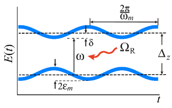
Figure 1: Schematic illustration of magnetic resonance in a modulated longitudinal field. The Zeeman splitting, $\Delta_{Z}$, oscillates in time with a small magnitude, $\varepsilon_{\scriptscriptstyle m}$, and frequency, $\omega_{\scriptscriptstyle m}$.

Under the conditions (i), (ii) the classical Rabi resultRabi

$$P_{+\frac{1}{2}}(t)=\frac{\Omega_{{\scriptscriptstyle R}}^{2}}{\omega_{{\scriptscriptstyle 0}}^{2}}\sin^{2}\frac{\omega_{{\scriptscriptstyle 0}}t}{2},$$ (1)

for the oscillating population of the upper Zeeman level, which was empty at $t=0$, applies. Here

$$\omega_{{\scriptscriptstyle 0}}=\sqrt{\delta^{2}+\Omega_{{\scriptscriptstyle R}}^{2}}$$ (2)

is the oscillation frequency, and $\delta=\Delta_{{\scriptscriptstyle Z}}-\omega$ is a detuning of the driving frequency from resonance.

It is knownTownes ; Shirley that almost sinusoidal Rabi oscillations can also be excited in the domains of parameters where the conditions (i) and (ii) are not met. One exampleTownes is the multiphoton Rabi oscillations which develop when the driving frequency is close to

$$\omega^{(p)}=\frac{\Delta_{\scriptscriptstyle Z}}{2p+1},$$ (3)

where $p$ is positive integer. Another exampleShirley is realized in the domain of frequencies

$$\omega\sim\Omega_{\scriptscriptstyle R}\gg\Delta_{\scriptscriptstyle Z}.$$ (4)

Existence of the domain Eq. (4) requires a strong driving field $B_{\scriptscriptstyle 1}\gg B_{\scriptscriptstyle 0}$, which is quite unusual for magnetic resonance.

The main point of the present paper is that the entire spectrum of regimes of the Rabi oscillations can be realized when conditions (i) and (ii) still apply, but the longitudinal field contains a small slowly oscillating component, ${\bf z}B_{{\scriptscriptstyle 2}}(t)$, where $B_{\scriptscriptstyle 2}\ll B_{\scriptscriptstyle 0}$. In other words, we will assume that the Zeeman splitting, $\Delta_{\scriptscriptstyle Z}$, has a time dependent correction,

$$\varepsilon(t)=g\mu_{{\scriptscriptstyle 0}}B_{{\scriptscriptstyle 2}}(t),$$ (5)

and study how the classical result Eq. (1) is affected by this correction. We will demonstrate that even when the magnitude of the correction is much smaller than $\Delta_{\scriptscriptstyle Z}$ and it oscillates with a frequency much smaller than $\Delta_{\scriptscriptstyle Z}$, see Fig. 1, its effect on the Rabi oscillations can still be dramatic. To prove this statement in Sect. II we map a weakly and resonantly driven two-level system with modulation onto a strongly driven system without modulation. In sections III, IV, and V we make use of this mapping to study how different regimes of spin dynamics emerge in different limits of modulation, namely, fast (compared to $\Omega_{\scriptscriptstyle R}$) modulation, strong (compared to $\Omega_{\scriptscriptstyle R}$) modulation, and near-resonant modulation (with frequency $\approx\Omega_{\scriptscriptstyle R}$). In Sect. VI we report the results of the experimental test of theoretical predictions. NMR measurements on protons in water have advantage that, without modulation, the pattern of Rabi oscillations could be observed over many periods. By applying the modulation pulse with varying frequency and magnitude, we were able to reproduce the above three regimes of spin dynamics. Concluding remarks are presented in Sect. VII.

II Mapping onto a strongly driven system without modulation

The time evolution of the amplitudes $C_{+\frac{1}{2}}$ and $C_{-\frac{1}{2}}$ of two spin orientations is governed by the system of equations

$$i{\dot{C}}_{+\frac{1}{2}}=\frac{\Delta_{{\scriptscriptstyle Z}}+\varepsilon(t)}{2}C_{+\frac{1}{2}}+\Omega_{{\scriptscriptstyle R}}C_{-\frac{1}{2}}\cos\omega t,$$ (6)

$$i{\dot{C}}_{-\frac{1}{2}}=-\frac{\Delta_{{\scriptscriptstyle Z}}+\varepsilon(t)}{2}C_{-\frac{1}{2}}+\Omega_{{\scriptscriptstyle R}}C_{+\frac{1}{2}}\cos\omega t.$$ (7)

In the absence of modulation, $\varepsilon(t)=0$, it is convenient to reduce this system to a single second-order differential equation by introducing, instead of $C_{+\frac{1}{2}}$ and $C_{-\frac{1}{2}}$, the combinations

$$A_{+}=C_{+\frac{1}{2}}+C_{-\frac{1}{2}},~{}~{}~{}~{}~{}A_{-}=C_{+\frac{1}{2}}-C_{-\frac{1}{2}}.$$ (8)

The system of equations for the new amplitudes reads

$$i{\dot{A}_{+}}=\frac{\Delta_{{\scriptscriptstyle Z}}}{2}A_{-}+\Omega_{{\scriptscriptstyle R}}A_{+}\cos\omega t,$$ (9)

$$i{\dot{A}_{-}}=\frac{\Delta_{{\scriptscriptstyle Z}}}{2}A_{+}-\Omega_{{\scriptscriptstyle R}}A_{-}\cos\omega t.$$ (10)

Upon expressing $A_{-}$ from Eq. (9) and substituting it into Eq. (10), we arrive at the sought equation

$${\ddot{A}_{+}}+\Bigl{[}-i\omega\Omega_{{\scriptscriptstyle R}}\sin\omega t+\Omega_{{\scriptscriptstyle R}}^{2}\cos^{2}\omega t+\frac{\Delta_{{\scriptscriptstyle Z}}^{2}}{4}\Bigr{]}A_{+}\!=0.$$ (11)

Assume now that the modulation is present, but, due to the weakness of the ac field, $\Omega{{\scriptscriptstyle R}}\ll\Delta_{{\scriptscriptstyle Z}}$, the system Eqs. (6), (7) can be treated within the rotating-wave approximation (RWA). This amounts to the replacement of $\cos\omega t$ by $\frac{1}{2}e^{-i\omega t}$ in Eq. (6), and by $\frac{1}{2}e^{i\omega t}$ in Eq. (7). Then, upon standard transformation into the rotating system

$$C_{+\frac{1}{2}}(t)=D_{+\frac{1}{2}}(t)e^{-\frac{i}{2}\omega t},~{}~{}~{}C_{-\frac{1}{2}}(t)=D_{-\frac{1}{2}}(t)e^{\frac{i}{2}\omega t},$$ (12)

these equations take the form

$$i{\dot{D}}_{+\frac{1}{2}}=\frac{\delta+\varepsilon(t)}{2}D_{+\frac{1}{2}}+\frac{\Omega_{{\scriptscriptstyle R}}}{2}D_{-\frac{1}{2}},$$ (13)

$$i{\dot{D}}_{-\frac{1}{2}}=-\frac{\delta+\varepsilon(t)}{2}D_{-\frac{1}{2}}+\frac{\Omega_{{\scriptscriptstyle R}}}{2}D_{+\frac{1}{2}}.$$ (14)

As a next step, we express $D_{-\frac{1}{2}}$ from Eq. (13) and substitute it into Eq. (14). This leads to the following second-order differential equation for $D_{+\frac{1}{2}}$

$${\ddot{D}}_{+\frac{1}{2}}+\Bigl{[}i\frac{\dot{\varepsilon}(t)}{2}+\frac{(\delta+\varepsilon)^{2}+\Omega_{{\scriptscriptstyle R}}^{2}}{4}\Bigr{]}D_{+\frac{1}{2}}=0.$$ (15)

At this point we assume that the modulation is sinusoidal,

$$\varepsilon(t)=\varepsilon_{{\scriptscriptstyle m}}\cos\omega_{{\scriptscriptstyle m}}t,$$ (16)

and make the key observation that, for $\delta=0$, Eq. (15) reduces to Eq. (11) upon replacement

$$\Omega_{{\scriptscriptstyle R}}\rightarrow\Delta_{{\scriptscriptstyle Z}},~{}~{}\varepsilon_{{\scriptscriptstyle m}}\rightarrow 2\Omega_{{\scriptscriptstyle R}},~{}~{}\omega_{{\scriptscriptstyle m}}\rightarrow\omega.$$ (17)

This mapping provides an important insight into the effect of modulation of the longitudinal field on magnetic resonance. Indeed, Eq. (11) captures the time evolution of the populations $|C_{+\frac{1}{2}}(t)|^{2}$ and $|C_{-\frac{1}{2}}(t)|^{2}$ when the ac drive is not weak, i.e., $\Omega_{{\scriptscriptstyle R}}\gtrsim\Delta_{{\scriptscriptstyle Z}}$, so that RWA does not apply. On the other hand, Eq. (15) describes the spin dynamics with weak ac drive, but in the presence of the modulation. Solutions of Eq. (11), the structure of which is dictated by the Floquet theorem, were analyzed in a great number of papers starting from pioneering worksTownes ; Shirley . Therefore, the approaches developed for a driven spin-$\frac{1}{2}$ system without modulation can be utilized for the case when the modulation is present.

For example, in the absence of modulation, resonant drive of the spin-$\frac{1}{2}$ system corresponds to the condition $\omega=\Delta_{\scriptscriptstyle Z}$. Then from Eq. (17) we conclude that the effect of modulation on the Rabi oscillations is most pronounced when the modulation frequency, $\omega_{{\scriptscriptstyle m}}$, is close to the Rabi frequency, $\Omega_{{\scriptscriptstyle R}}$. This sensitivity was previously pointed out in Refs. rotary, ; DoublyDriven, ; Greenberg1, ; Greenberg2, ; Saiko1, .

A less obvious consequence of the mapping Eq. (17) is that, upon increasing the modulation strength, $\varepsilon_{{\scriptscriptstyle m}}$, the Rabi oscillations become sensitive to the modulation for modulation frequencies close to

$$\omega^{(p)}_{{\scriptscriptstyle m}}=\frac{\Omega_{{\scriptscriptstyle R}}}{2p+1}.$$ (18)

Condition Eq. (18) implies that the modulation affects the Rabi oscillations when the modulation period contains an odd number of the Rabi periods. This condition is an analog of the condition for multiphoton resonances in a driven two-level systemTownes which take place at ac driving frequencies $\omega\approx\omega^{(p)}$, where $\omega^{(p)}$ is given by Eq. (3).

Despite the fact that Eqs. (11) and (15) can be formally mapped onto each other, the physical phenomena that they describe are vastly different. For the most prominent example, $\omega\approx\Delta_{\scriptscriptstyle Z}$, Eq. (11) describes the Rabi oscillations of the populations of the Zeeman levels, while Eq. (15) describes slow envelope of these oscillations, which emerges due to modulation, $\varepsilon(t)$, of $\Delta_{{\scriptscriptstyle Z}}$. Formally, the difference stems from the initial conditions, which must be imposed on the solutions of Eqs. (11) and (15). If, for example, at $t=0$ the spin points down, then the initial conditions for Eq. (11) read

$$A_{+}(0)=1,~{}~{}~{}{\dot{A}_{+}}(0)=i\left(\frac{\Delta_{{\scriptscriptstyle Z}}}{2}-\Omega_{{\scriptscriptstyle R}}\right).$$ (19)

For the same initial state, the initial conditions for Eq. (15) have the form

$$D_{+\frac{1}{2}}(0)=0,~{}~{}~{}{\dot{D}}_{+\frac{1}{2}}(0)=-i\frac{\Omega_{{\scriptscriptstyle R}}}{2}.$$ (20)

Below we study the spin dynamics, $P_{+\frac{1}{2}}(t)$, in different domains of modulation frequencies and magnitudes.

III Fast modulation: $\omega_{\scriptscriptstyle m}\gg\Omega_{\scriptscriptstyle R}$.

Qualitatively, it is clear that weak modulation $\varepsilon_{\scriptscriptstyle m}\ll\omega_{\scriptscriptstyle m}$ averages out if the modulation frequency is much bigger than $\Omega_{\scriptscriptstyle R}$. Then the Rabi oscillations remain unaffected. Nontrivial modification of the Rabi oscillations takes place when both $\omega_{\scriptscriptstyle m}$ and $\varepsilon_{\scriptscriptstyle m}$ are much bigger than $\Omega_{\scriptscriptstyle R}$. For conventional magnetic resonance this regime corresponds to $\omega\gg\Delta_{\scriptscriptstyle Z}$ and $\Omega_{\scriptscriptstyle R}\gg\Delta_{\scriptscriptstyle Z}$, see Eq. (17), i.e., $B_{\scriptscriptstyle 1}\gg B_{\scriptscriptstyle 0}$, which is exotic. Fast modulation, on the other hand, is fully compatible with $B_{\scriptscriptstyle 1}\ll B_{\scriptscriptstyle 0}$.

For simplicity we will consider the case of zero detuning, $\delta=0$. To analyze the limit $\omega_{{\scriptscriptstyle m}}\gg\Omega_{{\scriptscriptstyle R}}$ it is convenient to introduce the new variables

$${\tilde{D}}_{-\frac{1}{2}}\!=\!D_{-\frac{1}{2}}(t)e^{\frac{i\varepsilon_{\scriptscriptstyle m}}{2\omega_{\scriptscriptstyle m}}\sin\omega_{\scriptscriptstyle m}t},$$

$${\tilde{D}}_{+\frac{1}{2}}\!=\!D_{+\frac{1}{2}}(t)e^{\frac{-i\varepsilon_{\scriptscriptstyle m}}{2\omega_{\scriptscriptstyle m}}\sin\omega_{\scriptscriptstyle m}t},$$ (21)

and to rewrite the system Eqs. (13), (14) as

$$i{\dot{\tilde{D}}}_{-\frac{1}{2}}=\frac{\Omega_{\scriptscriptstyle R}}{2}e^{\frac{i\varepsilon_{\scriptscriptstyle m}}{\omega_{\scriptscriptstyle m}}\sin\omega_{\scriptscriptstyle m}t}{\tilde{D}}_{+\frac{1}{2}},$$

$$i{\dot{\tilde{D}}}_{+\frac{1}{2}}=\frac{\Omega_{\scriptscriptstyle R}}{2}e^{-\frac{i\varepsilon_{\scriptscriptstyle m}}{\omega_{\scriptscriptstyle m}}\sin\omega_{\scriptscriptstyle m}t}{\tilde{D}}_{-\frac{1}{2}}.$$ (22)

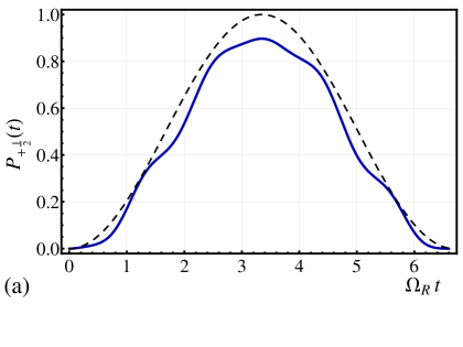
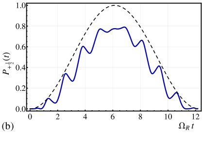
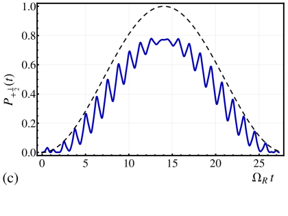
Figure 2: Fast modulation regime, $\omega_{\scriptscriptstyle m}\gg\Omega_{\scriptscriptstyle R}$. Modulation causes slowing down of the Rabi oscillations, which are plotted with dashed lines from Eq. (24) for $\omega_{\scriptscriptstyle m}=5\Omega_{\scriptscriptstyle R}$ and three values of the ratio $\frac{\varepsilon_{\scriptscriptstyle m}}{\omega_{\scriptscriptstyle m}}$: (a) $0.5$, (b) $1.5$, (c) $2$. Correction Eq. (III) gives rise to the fast component of the Rabi oscillations. The probability, $P_{+\frac{1}{2}}(t)$, with fast component taken into account is shown with full lines.

​​If we now replace $\exp{\bigl{(}\pm\frac{i\varepsilon_{\scriptscriptstyle m}}{\omega_{\scriptscriptstyle m}}\sin\omega_{\scriptscriptstyle m}t}\bigr{)}$ by the time average, $J_{\scriptscriptstyle 0}\!\!\left(\!\frac{\varepsilon_{\scriptscriptstyle m}}{\omega_{\scriptscriptstyle m}}\!\right)$, where $J_{\scriptscriptstyle 0}(z)$ is a zero-order Bessel function, the system Eq. (III) will readily yield

$${\tilde{D}}_{-\frac{1}{2}}\!=\!\cos\left(\frac{\Omega_{\scriptscriptstyle R}}{2}J_{\scriptscriptstyle 0}\!\!\left(\!\frac{\varepsilon_{\scriptscriptstyle m}}{\omega_{\scriptscriptstyle m}}\!\right)t\right)\!,~{}{\tilde{D}}_{+\frac{1}{2}}\!=-i\!\sin\left(\frac{\Omega_{\scriptscriptstyle R}}{2}J_{\scriptscriptstyle 0}\!\!\left(\!\frac{\varepsilon_{\scriptscriptstyle m}}{\omega_{\scriptscriptstyle m}}\!\right)t\right)\!,$$ (23)

so that

$$P_{+\frac{1}{2}}(t)=\sin^{2}\left(\frac{\Omega_{\scriptscriptstyle R}}{2}J_{\scriptscriptstyle 0}\!\!\left(\!\frac{\varepsilon_{\scriptscriptstyle m}}{\omega_{\scriptscriptstyle m}}\!\right)t\right).$$ (24)

The latter expression suggests that the effect of fast modulation, $\omega_{\scriptscriptstyle m}\gg\Omega_{\scriptscriptstyle R}$, on the Rabi oscillations is the reduction of their frequency by a factor $J_{\scriptscriptstyle 0}\!\!\left(\!\frac{\varepsilon_{\scriptscriptstyle m}}{\omega_{\scriptscriptstyle m}}\!\right)$. The reduction is significant when the modulation amplitude, $\varepsilon_{\scriptscriptstyle m}$, is of the order of $\omega_{\scriptscriptstyle m}$.

The remaining task is to demonstrate that, for arbitrary modulation strength, $\varepsilon_{\scriptscriptstyle m}$, the condition $\omega_{\scriptscriptstyle m}\gg\Omega_{\scriptscriptstyle R}$ justifies the replacement of $\exp{\bigl{(}\pm\frac{i\varepsilon_{\scriptscriptstyle m}}{\omega_{\scriptscriptstyle m}}\sin\omega_{\scriptscriptstyle m}t}\bigr{)}$ by $J_{\scriptscriptstyle 0}\!\!\left(\!\frac{\varepsilon_{\scriptscriptstyle m}}{\omega_{\scriptscriptstyle m}}\!\right)$. For this purpose we consider the correction to ${\tilde{D}}_{+\frac{1}{2}}$ coming from higher harmonics of $\exp{\bigl{(}\frac{i\varepsilon_{\scriptscriptstyle m}}{\omega_{\scriptscriptstyle m}}\sin\omega_{\scriptscriptstyle m}t}\bigr{)}$. It is convenient to cast this correction in the form

$${\tilde{D}}_{+\frac{1}{2}}+i\sin\left(\frac{\Omega_{\scriptscriptstyle R}}{2}J_{\scriptscriptstyle 0}\!\!\left(\!\frac{\varepsilon_{\scriptscriptstyle m}}{\omega_{\scriptscriptstyle m}}\!\right)t\right)$$

$$=-\frac{i\Omega_{\scriptscriptstyle R}}{2\omega_{\scriptscriptstyle m}}\int_{0}^{\omega_{\scriptscriptstyle m}t}\!\!d\phi\left[e^{-\frac{i\varepsilon_{\scriptscriptstyle m}}{\omega_{\scriptscriptstyle m}}\sin\phi}-\!\!J_{\scriptscriptstyle 0}\!\!\left(\!\frac{\varepsilon_{\scriptscriptstyle m}}{\omega_{\scriptscriptstyle m}}\!\right)\right]\cos\eta\phi,$$ (25)

where we introduced a small parameter

$$\eta=\frac{\Omega_{\scriptscriptstyle R}}{2\omega_{\scriptscriptstyle m}}J_{\scriptscriptstyle 0}\!\!\left(\!\frac{\varepsilon_{\scriptscriptstyle m}}{\omega_{\scriptscriptstyle m}}\!\right)\ll 1.$$ (26)

There is a small prefactor in front of the integral. Still one has to check that the integral does not grow at large $\omega_{\scriptscriptstyle m}t$. Suppose that $\omega_{\scriptscriptstyle m}t=2\pi N$. Then the integration over $N$ modulation periods can be reduced to a single integral from $0$ to $2\pi$ in which $\cos\eta\phi$ is replaced by

$$\sum_{n=0}^{N}\!\cos\eta(\phi-2\pi n)=\frac{\cos\eta\phi}{2}\left(\!\frac{\sin 2\pi\eta N}{\tan\pi\eta}\!+\!\cos 2\pi\eta N+1\!\right)$$

$$\hskip 7.11317pt+\frac{\sin\eta\phi}{2}\left(\frac{1-\cos 2\pi\eta N}{\tan\pi\eta}+\sin 2\pi\eta N\right)\!.$$ (27)

We see that for $N<\eta^{-1}$ the first term grows with $N$. Moreover, this term is much bigger than the second term. However, the correction Eq. (III) is determined by the second term in Eq. (III). The reason is that the first term does not depend on $\phi$ with accuracy $\eta$. On the other hand, the part of the first term which is independent of $\phi$ does not contribute to the correction Eq. (III). This is because the integral from this part is zero. The second term in Eq. (III), by virtue of smallness of $\eta$, can be replaced by $\frac{\phi}{\pi}\sin^{2}\pi\eta N$, so it remains finite at large $N$. This proves that, even for strong modulation, the correction Eq. (III) is $\sim\Omega_{\scriptscriptstyle R}/\omega_{\scriptscriptstyle m}$. In terms of the probability $P_{+\frac{1}{2}}(t)$, the correction Eq. (III) gives rise to a fast component, as illustrated in Fig. 2.

IV Strong modulation: $\varepsilon_{\scriptscriptstyle m}\gg\Omega_{\scriptscriptstyle R}\gg\omega_{\scriptscriptstyle m}$

For strong modulation, $\varepsilon_{\scriptscriptstyle m}\gg\Omega_{\scriptscriptstyle R}$, the term $\Omega_{\scriptscriptstyle R}^{2}$ in Eq. (15) is small compared to $\varepsilon^{2}$, which suggests that Rabi oscillations do not develop. However, if the modulation is slow enough, and the detuning, $\delta$, is much smaller than $\Omega_{\scriptscriptstyle R}$, the term $\Omega_{\scriptscriptstyle R}^{2}$ will be dominant during short (compared to $\omega_{\scriptscriptstyle m}^{-1}$) time intervals near

$$t=t_{\scriptscriptstyle k}=\left(\frac{\pi}{2}+\pi k\right)\omega_{\scriptscriptstyle m}^{-1},$$ (28)

when $\varepsilon(t)$ passes through zero. Within these intervals we can set $t=t_{\scriptscriptstyle k}+t_{1}$ and expand $\varepsilon(t)$ with respect to $t_{1}$. Then Eq. (15) assumes the form

$${\ddot{D}}_{+\frac{1}{2}}+\Biggl{[}i\frac{\varepsilon_{\scriptscriptstyle m}\omega_{\scriptscriptstyle m}}{2}+\frac{\varepsilon_{\scriptscriptstyle m}^{2}\omega_{\scriptscriptstyle m}^{2}t_{\scriptscriptstyle 1}^{2}+\Omega_{{\scriptscriptstyle R}}^{2}}{4}\Biggr{]}D_{+\frac{1}{2}}=0,$$ (29)

where we assumed for definitiveness that $k$ is odd.

Solution of Eq. (29) can be expressed in terms of parabolic cylinder functionsTranscendental

$$D_{+\frac{1}{2}}(t_{\scriptscriptstyle 1})=f_{\scriptscriptstyle 1}\,{\cal D}_{\nu}\!\left(\!e^{\frac{\pi i}{4}}\frac{t_{\scriptscriptstyle 1}}{\tau}\!\right)+f_{\scriptscriptstyle 2}\,{\cal D}_{\nu}\!\left(\!\!-e^{\frac{\pi i}{4}}\frac{t_{\scriptscriptstyle 1}}{\tau}\!\right)\!,$$ (30)

where the characteristic time, $\tau$, is given by

$$\tau=\frac{1}{(\varepsilon_{\scriptscriptstyle m}\,\omega_{\scriptscriptstyle m})^{1/2}},$$ (31)

and parameter $\nu$ is defined as

$$\nu=-i~{}\frac{\Omega_{\scriptscriptstyle R}^{2}}{4\varepsilon_{\scriptscriptstyle m}\,{\omega_{\scriptscriptstyle m}}}.$$ (32)

Expansion of $\varepsilon(t)$ is justified under the condition, $\omega_{\scriptscriptstyle m}\tau\ll 1$, which reduces to $\varepsilon_{\scriptscriptstyle m}\gg\omega_{\scriptscriptstyle m}$. With regard to parameter, $\nu$, it can be presented as a product $|\nu|=\left(\frac{\Omega_{\scriptscriptstyle R}}{2\varepsilon_{\scriptscriptstyle m}}\right)^{2}\!\!\left(\frac{\varepsilon_{\scriptscriptstyle m}}{\omega_{\scriptscriptstyle m}}\right)$. The first factor of this product is small, while the second factor is large. This means that in the domain $\varepsilon_{\scriptscriptstyle m}\gg\Omega_{\scriptscriptstyle R}\gg\omega_{\scriptscriptstyle m}$ the value $|\nu|$ can be both large and small. The magnitude of $|\nu|$ determines the angle of the spin rotation as $\varepsilon(t)$ passes through zero. To see this, assume that at moment $t=t_{\scriptscriptstyle k}$ the spin points down. Then the constants $f_{\scriptscriptstyle 1}$, $f_{\scriptscriptstyle 2}$ in Eq. (30) can be found from the initial conditions Eq. (20), yielding

$$D_{+\frac{1}{2}}(t_{\scriptscriptstyle 1})\!=\frac{|\nu|^{1/2}\,\,e^{-\frac{3\pi i}{4}}}{2\,{\cal D}_{\nu}^{\prime}(0)}\left[{\cal D}_{\nu}\!\left(\!e^{\frac{\pi i}{4}}\frac{t_{\scriptscriptstyle 1}}{\tau}\right)-{\cal D}_{\nu}\!\left(\!\!-e^{\frac{\pi i}{4}}\frac{t_{\scriptscriptstyle 1}}{\tau}\right)\right]\!,$$ (33)

where ${\cal D}_{\nu}^{\prime}(0)$ is the derivative of ${\cal D}_{\nu}(z)$ at $z=0$. The dependence of ${\cal D}_{\nu}^{\prime}(0)$ on $\nu$ can be established from the integral representation of the parabolic cylinder functionTranscendental

$${\cal D}_{\nu}^{\prime}(0)=\biggl{(}\frac{2}{\pi}\biggr{)}^{1/2}2\,^{\nu/2}\sin\left(\frac{\pi\nu}{2}\right)\Gamma\left(\frac{\nu}{2}+1\right)\!.$$ (34)

Here $\Gamma(z)$ is the gamma-function. The probability $P_{+\frac{1}{2}}(t_{\scriptscriptstyle 1})$ contains $|{\cal D}_{\nu}^{\prime}(0)|^{2}$, which, using the properties of the gamma-function, can be simplified to

$$|{\cal D}_{\nu}^{\prime}(0)|^{2}=|\nu|\sinh\!\left(\!\frac{\pi|\nu|}{2}\!\right).$$ (35)

Substituting Eq. (35) into Eq. (33), we arrive at the final result

$$P_{+\frac{1}{2}}(t_{\scriptscriptstyle 1})=\frac{1}{4\sinh\!\left(\!\frac{\pi|\nu|}{2}\!\right)}\left|{\cal D}_{\nu}\!\left(\!e^{\frac{\pi i}{4}}\frac{t_{\scriptscriptstyle 1}}{\tau}\!\right)-{\cal D}_{\nu}\!\left(\!\!-e^{\frac{\pi i}{4}}\frac{t_{\scriptscriptstyle 1}}{\tau}\!\right)\right|^{2}.$$ (36)

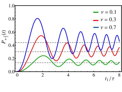
Figure 3: Strong modulation regime, $\varepsilon_{\scriptscriptstyle m}\gg\Omega_{\scriptscriptstyle R}\gg\omega_{\scriptscriptstyle m}$. Spin dynamics persists only during short intervals $|t-t_{\scriptscriptstyle k}|\sim\tau\ll\omega_{\scriptscriptstyle m}^{(-1)}$ around the moments, $t_{\scriptscriptstyle k}$, when modulation passes through zero. Probability, $P_{+\frac{1}{2}}$, is plotted from Eq. (36) versus dimensionless time $(t-t_{\scriptscriptstyle k})/\tau$ for three values of parameter $|\nu|$, Eq. (32), describing the strength of the ac drive. Green, red, and blue curves correspond to the values $|\nu|=0.1$, $|\nu|=0.3$, and $|\nu|=0.7$, respectively.

In Fig. 3 the dependence $P_{+\frac{1}{2}}(t_{\scriptscriptstyle 1})$ is plotted from Eq. (36) for different values of the parameter $|\nu|$. We see that, starting from zero, $P_{+\frac{1}{2}}(t_{\scriptscriptstyle 1})$ oscillates with $t_{\scriptscriptstyle 1}$, and, finally, saturates at $t_{\scriptscriptstyle 1}\gg\tau$ at some finite value, $P_{+\frac{1}{2}}(\infty)$. To find $P_{+\frac{1}{2}}(\infty)$ we use the large-$z$ asymptote of the parabolic cylinder functionTranscendental , ${\cal D}_{\nu}(z)\sim z^{\nu}\exp{\left(\frac{1}{4}z^{2}\right)}$, and the fact that the asymptotes of ${\cal D}_{\nu}(z)$ and ${\cal D}_{\nu}(-z)$ differ by $\exp(i\pi\nu)=\exp(-\pi|\nu|)$. This allows to find the saturation level of the numerator to be $4\sinh^{2}\!\left(\frac{\pi|\nu|}{4}\right)\exp\left(\!-\frac{\pi|\nu|}{2}\right)$. Subsequently, the saturation level of $P_{+\frac{1}{2}}$ assumes the form

$$P_{+\frac{1}{2}}(\infty)=\frac{1-e^{-\pi|\nu|}}{2}.$$ (37)

The meaning of the result Eq. (37) is transparent. If the driving field is weak, so that $|\nu|\ll 1$, we have $P_{+\frac{1}{2}}(\infty)\ll 1$, which implies that the spin pointing down at $t=t_{\scriptscriptstyle k}$ retains its orientation throughout the entire interval $t_{\scriptscriptstyle k+1}-t_{\scriptscriptstyle k}=\frac{\pi}{\omega_{\scriptscriptstyle m}}$. If the driving field is strong, so that $|\nu|\gg 1$, the spin, during the short time $\ll\frac{\pi}{\omega_{\scriptscriptstyle m}}$, will rotate to the position $P_{+\frac{1}{2}}\approx P_{-\frac{1}{2}}\approx\frac{1}{2}$, i.e., will point along the $x$-axis, and spend in this position the remaining part of the interval $t_{\scriptscriptstyle k+1}-t_{\scriptscriptstyle k}$.

V Weak resonant modulation: $\omega_{{\scriptscriptstyle m}}\approx\Omega_{{\scriptscriptstyle R}};\varepsilon_{{\scriptscriptstyle m}}\ll\Omega_{{\scriptscriptstyle R}}.$

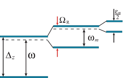
Figure 4: Schematic illustration of the second-order Rabi oscillations emerging as a result of slow modulation of the static field, $B_{\scriptscriptstyle 0}$. Driving resonant ac field, splits the quasienergies by $\Omega_{\scriptscriptstyle R}$; modulation with frequency $\omega_{\scriptscriptstyle m}\approx\Omega_{\scriptscriptstyle R}$ leads to an additional splitting.

V.1 Qualitative picture

In Sect. II, based on the mapping Eq. (17), we concluded that Rabi oscillations are strongly sensitive to the modulation of the longitudinal field when $\omega_{\scriptscriptstyle m}$ is close to $\Omega_{\scriptscriptstyle R}$. It is illustrative to discuss the effect of modulation near this condition using the language of quasienergies. Within this language, without modulation, the presence of a resonant field with frequency $\omega\approx\Delta_{{\scriptscriptstyle Z}}$ results in a degeneracy of quasinenergies corresponding to Zeeman-split levels, see Fig. 4. Conventional Rabi oscillations emerge as a result of lifting this degeneracy (avoided crossing); the magnitude of the splitting of quasienergies is $\Omega_{{\scriptscriptstyle R}}$.

With periodic modulation, the Hamiltonian in the quasienergy representation remains time-dependent and the corresponding eigenstates are characterized by second-order quasienergies. When the frequency of modulation is close to $\Omega_{{\scriptscriptstyle R}}$, the first-order Rabi-split quasienergies become degenerate, leading to their additional splitting, see Fig. 4. The magnitude of this additional splitting is controlled by the modulation amplitude. In the time domain, this additional splitting manifests itself via second-order Rabi oscillations in the form of an envelope of the primary oscillations.

As we show in the next subsection, the shape of this envelope is very sensitive to the detuning, $\omega_{\scriptscriptstyle m}-\Omega_{\scriptscriptstyle R}$, of modulation frequency from the Rabi frequency, and to the detuning, $\delta$, of the driving frequency from the Zeeman splitting, $\Delta_{\scriptscriptstyle Z}$.

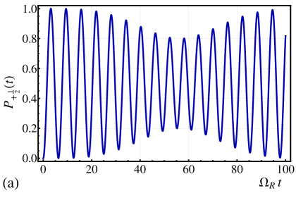
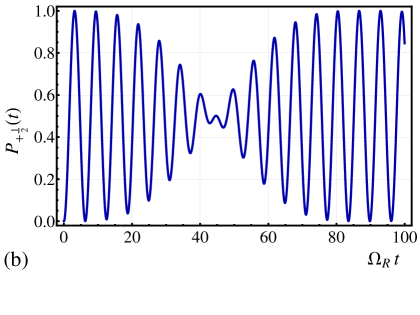
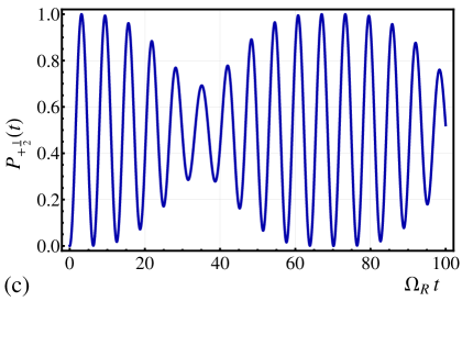
Figure 5: Evolution of the Rabi oscillation pattern with detuning of the modulation frequency from the Rabi frequency. Spin dynamics, $P_{+\frac{1}{2}}(t)$, under the resonant drive, $\delta=0$, is plotted from Eq. (V.2) for different dimensionless detunings, $\kappa$: $0.5$ (a), $1.0$ (b), and $1.5$ (c). The amplitude of modulation is $\varepsilon_{\scriptscriptstyle m}=0.1\,\Omega_{\scriptscriptstyle R}$. Upon increasing $\kappa$ the envelope develops (a), reaches maximum (b), and gradually vanishes (c).

V.2 The shape of the envelope

Near the condition $\omega_{\scriptscriptstyle m}=\Omega_{\scriptscriptstyle R}$ Eq. (15) can be solved in the resonant approximation, which amounts to keeping only two terms in the Floquet expansionShirley :

$$D_{+\frac{1}{2}}(t)=e^{i\lambda t}\Bigl{(}d_{{\scriptscriptstyle 0}}+d_{{\scriptscriptstyle-1}}e^{-i\omega_{{\scriptscriptstyle m}}t}\Bigr{)},$$ (38)

where $\lambda$ is the Floquet exponent. Substituting Eq. (38) into Eq. (15) and equating the resonant terms, we get the following system of coupled equations for the amplitudes $d_{{\scriptscriptstyle 0}}$, $d_{{\scriptscriptstyle-1}}$

$$\left(\Omega_{{\scriptscriptstyle R}}^{2}+\delta^{2}+\frac{\varepsilon_{{\scriptscriptstyle m}}^{2}}{2}-4\lambda^{2}\right)d_{{\scriptscriptstyle 0}}\!\!\! = \!\!\!-(\delta-\omega_{{\scriptscriptstyle m}})\varepsilon_{{\scriptscriptstyle m}}d_{{\scriptscriptstyle-1}},\hskip 28.45274pt$$

$$\left(\Omega_{{\scriptscriptstyle R}}^{2}\!+\!\delta^{2}\!+\!\frac{\varepsilon_{{\scriptscriptstyle m}}^{2}}{2}-4(\lambda-\omega_{{\scriptscriptstyle m}})^{2}\right)d_{{\scriptscriptstyle-1}}\!\!\! = \!\!\!-(\delta+\omega_{{\scriptscriptstyle m}})\varepsilon_{{\scriptscriptstyle m}}d_{{\scriptscriptstyle 0}}.$$ (39)

For vanishing modulation, $\varepsilon_{{\scriptscriptstyle m}}\rightarrow 0$, both left-hand sides in the system Eq. (V.2) turn to zero at the degeneracy point $\lambda=\frac{1}{2}\omega_{{\scriptscriptstyle m}}$, when the condition: $\omega_{{\scriptscriptstyle m}}=\omega_{{\scriptscriptstyle 0}}=\sqrt{\delta^{2}+\Omega_{{\scriptscriptstyle R}}^{2}}$ is met. At finite $\varepsilon_{{\scriptscriptstyle m}}$ the system yields the splitting of the Floquet exponents

$$\lambda_{{\scriptscriptstyle\pm}}=\frac{\omega_{{\scriptscriptstyle m}}}{2}\pm\frac{\varepsilon_{{\scriptscriptstyle m}}\,\Omega_{{\scriptscriptstyle R}}}{4\,\omega_{{\scriptscriptstyle 0}}}\sqrt{\kappa^{2}+1},$$ (40)

where we introduced a dimensionless deviation

$$\kappa=\frac{2(\omega_{{\scriptscriptstyle m}}-\omega_{{\scriptscriptstyle 0}})\omega_{{\scriptscriptstyle 0}}}{\varepsilon_{{\scriptscriptstyle m}}\,\Omega_{{\scriptscriptstyle R}}}.$$ (41)

of the modulation frequency from oscillation frequency, $\omega_{{\scriptscriptstyle 0}}$ and took into account that $|\omega_{{\scriptscriptstyle m}}-\omega_{{\scriptscriptstyle 0}}|\ll\omega_{{\scriptscriptstyle 0}}$. The steps leading from Eq. (38) to Eq. (40) are the same as the steps leading from Eq. (11) to the conventional Rabi oscillations Eq. (1). The difference arises when one substitutes $\lambda_{{\scriptscriptstyle+}}$, $\lambda_{{\scriptscriptstyle-}}$ into the system Eq. (V.2), finds two linearly independent solutions, $D_{+\frac{1}{2}}^{{\scriptscriptstyle+}}(t)$ and $D_{+\frac{1}{2}}^{{\scriptscriptstyle-}}(t)$, and requires that their sum satisfies the initial conditions Eq. (20). After that, upon calculating the occupation

$$P_{+\frac{1}{2}}(t)=\left|D_{+\frac{1}{2}}^{{\scriptscriptstyle+}}(t)+D_{+\frac{1}{2}}^{{\scriptscriptstyle-}}(t)\right|^{2},$$ (42)

one arrives at the following generalization of Eq. (1) to the case of modulated longitudinal field

$$P_{+\frac{1}{2}}(t)=\frac{1}{\kappa^{2}+1}\Biggl{[}\left(1{\bf-}\frac{\delta(\kappa\,\Omega_{{\scriptscriptstyle R}}+\delta)}{\omega_{\scriptscriptstyle 0}^{2}}\right)\sin^{2}\!\left(\!\frac{\omega_{\scriptscriptstyle 0}}{2}+\frac{\varepsilon_{\scriptscriptstyle m}\,\Omega_{\scriptscriptstyle R}}{4\,\omega_{\scriptscriptstyle 0}}\kappa\right)t+\frac{\Omega_{\scriptscriptstyle R}(\kappa\,\Omega_{\scriptscriptstyle R}+\delta)}{2\,\omega_{\scriptscriptstyle 0}^{2}\big{(}\sqrt{\kappa^{2}+1}-\kappa\big{)}}\sin^{2}\!\left(\!\frac{\omega_{\scriptscriptstyle 0}}{2}+\frac{\varepsilon{\scriptscriptstyle m}\,\Omega_{\scriptscriptstyle R}}{4\,\omega_{\scriptscriptstyle 0}}\left(\kappa-\sqrt{\kappa^{2}+1}\right)\right)t$$

$$\hskip 42.67912pt+\frac{\delta(\kappa\,\Omega_{\scriptscriptstyle R}+\delta)}{\omega_{\scriptscriptstyle 0}^{2}}\sin^{2}\!\left(\!\frac{\varepsilon_{\scriptscriptstyle m}\,\Omega_{\scriptscriptstyle R}}{4\,\omega_{\scriptscriptstyle 0}}\sqrt{\kappa^{2}+1}\!\right)t-\frac{\Omega_{\scriptscriptstyle R}(\kappa\,\Omega_{\scriptscriptstyle R}+\delta)}{2\,\omega_{\scriptscriptstyle 0}^{2}\big{(}\sqrt{\kappa^{2}+1}+\kappa\big{)}}\sin^{2}\!\left(\frac{\omega_{\scriptscriptstyle 0}}{2}+\frac{\varepsilon{\scriptscriptstyle m}\,\Omega_{\scriptscriptstyle R}}{4\,\omega_{\scriptscriptstyle 0}}\left(\kappa+\sqrt{\kappa^{2}+1}\right)\!\right)t\Biggr{]}.$$ (43)

We start the analysis of Eq. (V.2) from the case of zero detuning, $\delta=0$, when it simplifies considerably

$$P_{+\frac{1}{2}}(t)=\frac{1}{\kappa^{2}+1}\Biggl{[}\sin^{2}\!\left(\frac{\Omega_{\scriptscriptstyle R}}{2}+\frac{\varepsilon_{\scriptscriptstyle m}}{4}\kappa\!\right)\!t$$

$$+\frac{\kappa}{2\big{(}\!\sqrt{\kappa^{2}+1}-\kappa\big{)}}\sin^{2}\!\left(\!\frac{\Omega_{{\scriptscriptstyle R}}}{2}\!+\!\frac{\varepsilon_{\scriptscriptstyle m}}{4}\!\left(\!\kappa-\sqrt{\kappa^{2}+1}\!\right)\!\right)\!t$$

$$-\frac{\kappa}{2\big{(}\!\sqrt{\kappa^{2}+1}+\kappa\big{)}}\sin^{2}\!\left(\frac{\Omega_{{\scriptscriptstyle R}}}{2}\!+\!\frac{\varepsilon_{\scriptscriptstyle m}}{4}\!\left(\!\kappa+\!\sqrt{\kappa^{2}+1}\right)\!\right)\!t\Biggr{]}\!.\vspace{-1cm}$$ (44)

This expression is consistent with Ref. Saiko1, where a related quantity, namely the absorption of an external field by a resonantly driven spin-$\frac{1}{2}$ system in a modulated longitudinal field, has been studied.

The last two terms in Eq. (V.2) describe the second-order Rabi oscillations since their frequencies are split in agreement with qualitative picture Fig. 4. Naturally, taking the limit $\varepsilon_{\scriptscriptstyle m}\rightarrow 0$, we recover the conventional Rabi oscillations, $P_{+\frac{1}{2}}(t)=\sin^{2}\Bigl{(}\frac{\Omega_{\scriptscriptstyle R}t}{2}\Bigr{)}$, for any $\kappa$. A nontrivial feature of Eq. (V.2) is that exactly at $\omega_{\scriptscriptstyle m}=\Omega_{\scriptscriptstyle R}$, when $\kappa=0$, the last two terms cancel each other, i.e., the Rabi oscillations are unaffected by the modulation. Gradual development of the second-order oscillations upon increasing $\kappa$ is illustrated in Fig. 5. We see that the effect of modulation of longitudinal field is most pronounced at dimensionless detuning $\kappa\approx 1$, where the modulation of the Rabi oscillations is complete, see Fig. 5b. Upon further increasing $\kappa$, the effect of modulation vanishes above $\kappa=4$.

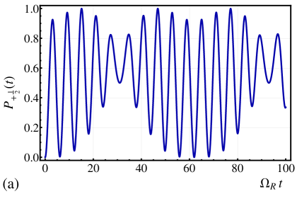
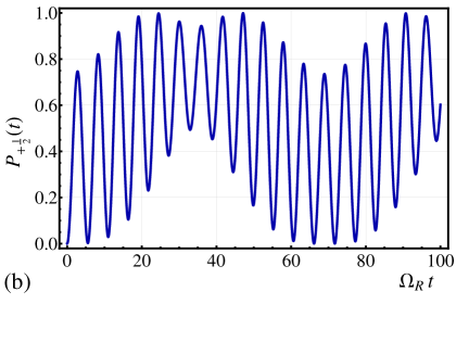
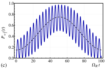
Figure 6: Regime of weak resonant modulation. Evolution of the Rabi oscillation pattern with detuning, $\delta$, of the driving frequency, $\omega$, from the level splitting, $\Delta_{\scriptscriptstyle Z}$. Spin dynamics, $P_{+\frac{1}{2}}(t)$, is plotted from Eq. (V.2) for three positive values of $\frac{\delta}{\Omega_{\scriptscriptstyle R}}$: $0.3$ (a), $0.6$ (b), and $1.4$ (c). The amplitude of modulation is $\varepsilon_{\scriptscriptstyle m}=0.15\,\Omega_{\scriptscriptstyle R}$; dimensionless detuning of the modulation frequency from $\Omega_{\scriptscriptstyle R}$ is $\kappa=1.0$. The pattern gradually evolves from envelope of the Rabi oscillations (a) to weak oscillations around the modulated baseline (c).

Beyond the resonant approximationSaiko1 , the difference, $\omega_{\scriptscriptstyle m}-\omega_{\scriptscriptstyle 0}$, in Eq. (41) acquires a correction $\sim\varepsilon_{\scriptscriptstyle m}^{2}/\Omega_{\scriptscriptstyle R}$, which is an analog of the Bloch-Siegert shiftBlochSiegert .

Solving Eq. (15) in the resonant approximation is also permitted when $\omega_{\scriptscriptstyle m}$ is close to $\omega^{(p)}_{\scriptscriptstyle m}=\frac{\Omega_{\scriptscriptstyle R}}{2p+1}$. Then the two resonating terms in the Floquet expansion are $d_{{\scriptscriptstyle 0}}$ and $d_{\scriptscriptstyle-(2p+1)}$. The splitting of the Floquet exponents, at the degeneracy point, $\lambda=\frac{\Omega_{{\scriptscriptstyle R}}}{2(2p+1)}$, takes place in the ($2p+1$)-th order in parameter $\varepsilon_{{\scriptscriptstyle m}}/\Omega_{{\scriptscriptstyle R}}$. The magnitude of the splitting can be obtained by readjusting notations in the expression for the width of multiphoton resonance obtained in Ref. Shirley,

$$\frac{\varepsilon_{\scriptscriptstyle m}^{(p)}}{2}=\Bigl{(}\frac{\varepsilon_{\scriptscriptstyle m}}{4}\Bigr{)}\Biggl{(}\frac{\varepsilon_{\scriptscriptstyle m}}{\omega^{(p)}_{\scriptscriptstyle m}}\Biggr{)}^{2p}\frac{1}{2^{2p-1}(p!)^{2}}.$$ (45)

In the domain $(\omega_{\scriptscriptstyle m}-\omega^{(p)})\sim\varepsilon_{\scriptscriptstyle m}^{(p)}$ Eq. (V.2) remains valid upon the replacement $\varepsilon_{\scriptscriptstyle m}\rightarrow\varepsilon_{\scriptscriptstyle m}^{(p)}$ and describes second-order multiphoton Rabi oscillations. Naturally, if the modulation is not purely sinusoidal but contains a harmonics,

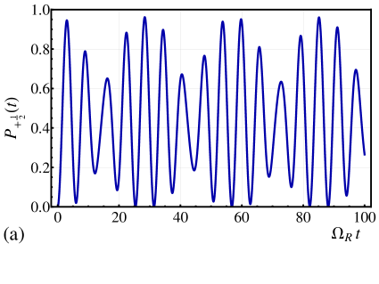
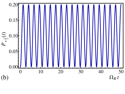
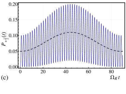
Figure 7: Same as Fig. 6 for three negative values of $\frac{\delta}{\Omega_{\scriptscriptstyle R}}$: $-0.2$ (a), $-2$ (b), and $-3$ (c). The pattern evolves from envelope (a) to homogeneous oscillations (b). Weak modulation of the baseline emerges only at large detuning (c).

say $l$, the envelope of the Rabi oscillations near $\omega_{\scriptscriptstyle m}=\Omega_{\scriptscriptstyle R}/l$ will already develop in the lowest order.

In the absence of modulation, finite detuning, $\delta$, of the driving frequency from the resonant frequency, $\Delta_{\scriptscriptstyle Z}$, leads to the reduction of the period of the Rabi oscillations and to the reduction of their amplitude, see Eqs. (1), (2). Remarkably, in the presence of modulation, near the condition $\omega_{\scriptscriptstyle m}=\Omega_{\scriptscriptstyle R}$, finite $\delta$ causes a new qualitative feature in the shape of the Rabi oscillations. Moreover, the effect of finite $\delta$ depends strongly on its sign.

In Fig. 6 we plot from Eq. (V.2) the evolution of the Rabi-oscillation pattern as $\delta$ increases in the positive direction, while parameter $\kappa$ is kept constant. We see that, while for small enough $\delta$, the prime effect of modulation is still a slow envelope of the oscillations, upon further increasing of $\delta$, the envelope gradually transforms into the oscillations of the baseline. At large enough $\delta$, Fig.  6c, these oscillations of the baseline dominate the Rabi-oscillation pattern.

As $\delta$ increases in the negative direction, see Fig. 7, the pattern of the Rabi oscillations evolves differently. At small $|\delta|$ modulation gives rise to the envelope, similar to the case of small positive $\delta$. However, at a certain $|\delta|$, see Fig  6b, the magnitude of the oscillations does not change with time at all, suggesting that the effects of two detunings, $\omega_{\scriptscriptstyle m}-\omega_{\scriptscriptstyle 0}$, and, $\omega-\Delta_{\scriptscriptstyle Z}$, cancel each other. Only upon further increase of $|\delta|$ the magnitude of oscillations decreases significantly, and they proceed around the slowly oscillating baseline, as shown in Fig.  6c. The plots in Figs. 6, 7 are drawn for the ratio $\varepsilon_{\scriptscriptstyle m}/\Omega_{\scriptscriptstyle R}=0.15$ and $\varepsilon_{\scriptscriptstyle m}/\Omega_{\scriptscriptstyle R}=0.2$, respectively, however general features of the modulation pattern depend weakly on this ratio.

VI Testing theory with NMR Experiment

The introduction of the longitudinal modulation field $\varepsilon(t)$ to investigate the general behavior of Rabi oscillations is highly compatible with conventional experimental NMR methods of inductive detection in thermally generated spin ensemblesBook2 . For the large $B_{\scriptscriptstyle 0}$ field generally required to achieve sufficient signal-to-noise ratio (SNR), the condition $B_{\scriptscriptstyle 1}\ll B_{\scriptscriptstyle 0}$ cannot be avoided, but the additional small-amplitude modulation field is easily realized (Fig. 8a). The three regimes elucidated in Sect. III, IV, and V were thus explored using straightforward NMR of protons in water (gyromagnetic ratio $\gamma=g\mu_{N}=4.25775$ kHz/G, where $\mu_{N}$ is the nuclear magneton). We needed only to take some additional care to ensure a stable and highly homogeneous rf driving field $B_{\scriptscriptstyle 1}$ across the sample, so that the pattern of Rabi oscillations could be observed over many periods.

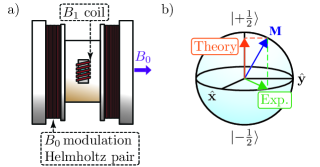
Figure 8: (Color online) a) A schematic of the NMR probe used in the experiments. A traditional NMR coil ($B_{\scriptscriptstyle 1}$) is accompanied by a $B_{\scriptscriptstyle 0}$ modulation Helmholtz pair that is coaxial with the $B_{\scriptscriptstyle 0}$ field. b) Graphical description of the relation between theoretical predictions and experimental NMR data. The theoretical predictions have the magnetization $\mathbf{M}$ projected onto the $z$-axis of the Bloch sphere. The experimental data is the projection of the magnetization onto the $xy$-plane of the Bloch sphere. Eq. (46) relates the theory to experiment.

All experiments were performed in a horizontal-bore 2-Tesla superconducting magnet (Oxford Instruments). A conventional solenoidal single-coil transmit/recieve probe (5 turns, 1 cm diam and 2.5 cm long) was series-tuned with a capacitor to the proton Zeeman resonance at 88.8 MHz. A 50-$\Omega$ resistor in series with these elements provided a matching impedance to the transmit and receive amplifiers. This “low-Q” probe sacrifices some SNR for a robust and flat frequency response that is negligibly affected by the accompanying modulation fieldBook2 ; Book3 . The water sample is centered in and occupies about 25% of the coil volume; it is contained in small tube made of PTFE (Teflon^TM), which minimizes the magnetic-susceptibility difference between the sample and its immediate surroundings. Both the low filling factor and PTFE tube serve to enhance the $B_{\scriptscriptstyle 1}$-field homogeneity across the sample. The modulation field was provided by a 5-cm-radius Helmholtz pair (coaxial with the main $B_{\scriptscriptstyle 0}$ field) wound on a form that has the probe coil at its center (see Fig. 8a). A NMR spectrometer (Tecmag Redstone, model HF2-1RX) with two independent transmission channels was used to transmit pulses to both the 88.8 MHz proton probe and the 0-100 kHz modulation coils, and subsequently to acquire and digitize the free-induction-decay (FID) signal generated in the probe coil. The $B_{\scriptscriptstyle 1}$ rf pulse was amplified with a 2 kW amplifier (Tomco model BTO2000-AlphaSA) conventionally designed for solid-state NMR, but whose high output power allowed the coherent nutation of the proton spins through many Rabi-oscillation periods in a relatively short pulse time. The $B_{\scriptscriptstyle 0}$-modulation pulse was provided by a DC-50 kHz amplifier normally used for gradient coils in imaging applications (Techron AN7780); the inductance of the Helmholtz pair was matched to the gradient amplifier’s output specifications in order to minimize ring-down and associated cross-talk to the NMR coil.

The FID signals were acquired on resonance ($\delta=0$) in single-shot fashion (no signal averaging), and the FID signal strength was plotted vs. $B_{\scriptscriptstyle 1}$ pulse length. Each data point displayed is the result of examining the corresponding FID to determine the magnitude of the transverse magnetization at a fixed time delay $\approx 0.2$ ms from the end of the $B_{\scriptscriptstyle 1}$ rf pulse. The $B_{\scriptscriptstyle 1}$ and modulation pulses are essentially applied simultaneously, with the modulation pulse nominally starting at $\varepsilon(t)=0$ just as the $B_{\scriptscriptstyle 1}$ pulse starts. We assume that the $B_{\scriptscriptstyle 1}$-pulse amplitude is fixed and the pulse length is linearly related to the nutation angle of the proton spins. Because of slight transient changes in power delivered by the rf amplifier at the very beginning of the $B_{\scriptscriptstyle 1}$ pulse (minimized by using a low-Q probe), this linear relationship is most accurately observed for longer pulse times. Indeed, when we determine $\Omega_{\scriptscriptstyle R}$ experimentally using non-modulated data, we rely on measuring the average period of the later-time oscillations. With this caveat in mind, the plots we show below represent Rabi oscillations in the three modulation regimes of interest. To decrease the overall data acquisition time, the water sample contained dissolved copper sulfate (CuSO₄) to reduce the longitudinal relaxation time $T_{\scriptscriptstyle 1}$ to $\approx 100$ ms. One must generally wait at least several times $T_{\scriptscriptstyle 1}$ between FID acquisitions to allow the magnetization to recover to its characteristic thermal-equilibrium value. Intrinsic transverse relaxation (characterized by $T_{\scriptscriptstyle 2}$) is typically on the order of $T_{\scriptscriptstyle 1}$ in weakly interacting liquids. We observed transverse decoherence caused by residual inhomogeneity (characterized by $T_{\scriptscriptstyle 2}^{*}<T_{\scriptscriptstyle 2}$) in the $B_{\scriptscriptstyle 1}$ field, which manifests most clearly in our data as the overall decay of the non-modulated Rabi oscillations after many characteristic periods (see Figs. 9-11).

We note that the predictions made in Sections III-V are formulated in terms of the projection of the magnetization onto the $z$-axis of the Bloch sphere (see Fig. 8b). Rabi oscillations occur between the high- and low-energy states defined by $B_{\scriptscriptstyle 0}$, where the low-energy state has magnetization parallel to $B_{\scriptscriptstyle 0}$. However, the observable in a conventional NMR experiment is the projection of the magnetization onto the $xy$-plane of the Bloch sphere. Noting also that the initial conditions at time $t=0$ for our predictions have $P_{+\frac{1}{2}}(0)=0$, whereas the experiments have $P_{+\frac{1}{2}}(0)=1$, a simple transformation of the $z$-axis prediction to the $xy$-plane can be accomplished by

$$P_{\perp}=\sin\big{[}\arccos(2P_{+\frac{1}{2}}-1)\big{]}=2\sqrt{P_{+\frac{1}{2}}-P_{+\frac{1}{2}}^{2}}.$$ (46)

In Figs. 9-11 we display the experimentally measured transverse magnetization data represented by $P_{\perp}$ and compare them to theory by transforming the predictions according to Eq. (46). The initial peak of the non-modulated Rabi-oscillation data, which appears in black in each figure, is used to define $P_{\perp}=1$ and to normalize the corresponding modulated data.

Figure 9: (Color online) Rabi oscillations in the fast-modulation regime (green) compared to non-modulated data (black). Transverse spin projection $P_{\perp}$ is plotted vs. pulse length; the latter is linearly related to the nutation angle. a) The modulation amplitude $\varepsilon_{\scriptscriptstyle m}$ is small compared with $\omega_{\scriptscriptstyle m}$, and the modulated data show the expected small upward shift in the oscillation frequency. A fit of the modulated data to Eq. (24) is shown by the dashed red line. The experimentally determined values of the modulation frequency $\omega_{\scriptscriptstyle m}/2\pi\!=\!41.30\pm 0.01$ kHz, modulation amplitude $\varepsilon_{\scriptscriptstyle m}/2\pi\gamma\!=\!4.96\pm 0.06$ G, and the Rabi frequency $\Omega_{\scriptscriptstyle R}/2\pi\!=\!8.26\pm 0.05$ kHz (determined from the non-modulated data) are input as fixed parameters. The fit includes multiplication of Eq. (24) by $e^{-t/{T_{\scriptscriptstyle 2}^{*}}}$ to account for the overall decay; the fit then yields $T_{\scriptscriptstyle 2}^{*}=1.28$ $\pm 0.02$ ms. b) The modulation amplitude is large compared with $\omega_{\scriptscriptstyle m}$, and the oscillation frequency decreases significantly, in accordance with Eq. (24). Here, $\omega_{\scriptscriptstyle m}/2\pi\!=\!31.5\pm 0.01$ kHz and $\Omega_{\scriptscriptstyle R}/2\pi\!=\!3.10\pm 0.02$ kHz are experimentally determined. A fit that incorporates the correction of Eq. (III) is shown in red, from which $\varepsilon_{\scriptscriptstyle m}/2\pi\gamma\!=\!13.0\pm 0.1$ G is extracted; larger values of $\varepsilon_{\scriptscriptstyle m}$ were difficult to measure experimentally. The correction gives rise to the oscillations at $\omega_{m}$ that ride on top of the much slower Rabi oscillations. The weaker $B_{\scriptscriptstyle 1}$ produces negligible $T_{\scriptscriptstyle 2}^{*}$ decay.

We begin with the fast-modulation regime, $\omega_{\scriptscriptstyle m}\!\gg\!\Omega_{\scriptscriptstyle R}$, studied in Sect. III, The picture in the “rotating frame” that results from the application of the RWA, is that of an average nutation of the magnetization in the $yz$-plane, superimposed with much faster wiggles, which for small modulation amplitudes are transverse to the $yz$-plane. For larger modulation amplitudes, the wiggles move the magnetization appreciably along the surface of the Bloch sphere, giving rise to a time-average decrease in the component of the magnetization that is in the $yz$-plane and subject to a torque generated by $B_{\scriptscriptstyle 1}$. This leads directly to the slowing down of the Rabi nutation expressed by Eq. (24)Book1 . The wiggles also lead to the fast modulation component at $\omega_{\scriptscriptstyle m}$, expressed in Eq. (III), that is superimposed on the slowed-down Rabi oscillations. Fig. 9a demonstrates that the corresponding experiments are sensitive to even the small decrease in the effective Rabi frequency $\Omega_{\scriptscriptstyle R}J_{\scriptscriptstyle 0}\left(\frac{\varepsilon_{\scriptscriptstyle m}}{\omega_{\scriptscriptstyle m}}\right)$ that appears for weak modulation. We were able to fit this data with Eq. (24) multiplied by a a decaying exponential that accounts for the $T_{\scriptscriptstyle 2}^{*}$ decay. The Rabi frequency $\Omega_{\scriptscriptstyle R}$ and modulation amplitude $\varepsilon_{\scriptscriptstyle m}$ were experimentally determined, respectively, by examining the non-modulated data and by measuring the current in the modulation coils.

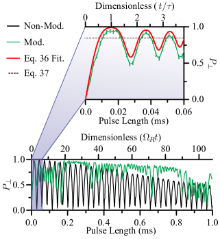
Figure 10: (Color online) Rabi oscillations in the strong-modulation regime (green) compared to non-modulated data (black). Transverse spin projection $P_{\perp}$ is plotted vs. pulse length; the latter is linearly related to the nutation angle. The lower part of the figure shows the complete data set. Data without modulation (black) yields a Rabi frequency $\Omega_{\scriptscriptstyle R}/2\pi\!=\!17.7\pm 0.1$ kHz. Data with modulation are shown in green; the applied modulation frequency was $\omega_{\scriptscriptstyle m}/2\pi\!=\!3.0\pm 0.1$ kHz. The critical regions near $\varepsilon(t)=0$ occur every $0.166$ ms and are characterized by non-trivial oscillation behavior; the first such region is shown expanded in the upper part of the figure. These early-time data show the decreasing oscillation period characteristic of the parabolic cylinder functions. The results of a fit (red) of the early-time data to Eq. (36) yields $\varepsilon_{\scriptscriptstyle m}/2\pi\gamma\ \!=\!7.0\pm 0.05$ G, which then leads to $|\nu|\!=\!0.9\pm 0.1$. An asymptote (dashed maroon) is calculated from Eq. (36) and is also shown. Well away from the zero-crossings of $\varepsilon(t)$, the magnetization continues to nutate in a more regular fashion; that it nutates at all is the result of not sufficiently satisfying the limit $\varepsilon_{\scriptscriptstyle m}\gg\Omega_{\scriptscriptstyle R}$.

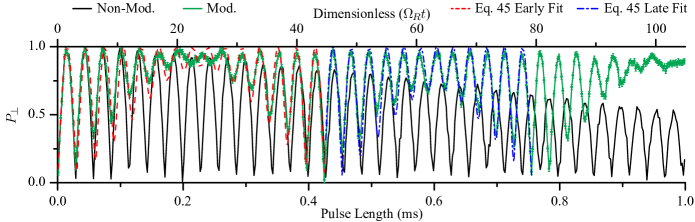
Figure 11: (Color online) Rabi oscillations in the regime of weak resonant modulation, showing definite beats that depend on the parameter $\kappa$. The Rabi frequency is found from the non-modulated data to be $\Omega_{\scriptscriptstyle R}/2\pi\!=\!16.7\!\pm\!0.7$ kHz. The sensitivity of the fit to small changes in the modulation frequency $\omega_{m}$ and experimental limitations led us to float most of the experimental parameters and to perform two separate fits of these data to Eq. (V.2) for the early-time (red dashed) and late-time (blue-dashed) portions of the overall acquisition. For the early-time fit, the extracted values are: $\Omega_{\scriptscriptstyle R}/2\pi\!=\!16.5\!\pm\!0.2$ kHz, $\varepsilon_{\scriptscriptstyle m}/2\pi\gamma\!=\!0.91\pm 0.04$ G, and $\omega_{\scriptscriptstyle m}/2\pi\!=\!17.56\!\pm\!0.05$, yielding $\kappa=0.54\pm 0.14$. for the late-time fit, the extracted values are: $\Omega_{\scriptscriptstyle R}/2\pi\!=\!17.0\!\pm\!0.2$ kHz, $\varepsilon_{\scriptscriptstyle m}/2\pi\gamma\!=\!1.2\pm 0.1$ G, and $\omega_{\scriptscriptstyle m}/2\pi\!=\!18.03\!\pm\!0.09$, yielding $\kappa=0.40\pm 0.12$. The data exhibit the beating envelope characteristic of this modulation regime.

Fig. 9b shows data in the regime of both fast and strong modulation $\varepsilon_{\scriptscriptstyle m},\,\omega_{\scriptscriptstyle m}\!\gg\!\Omega_{\scriptscriptstyle R}$, where corrections found in Eq. (III) become apparent. As predicted, the slowing-down effect on the Rabi oscillations now becomes pronounced, and the small modulation at frequency $\omega_{\scriptscriptstyle m}$ described by Eq. (III) rides on top of the envelope given by Eq. (24). A peculiar effect seen in the data and predicted in the theory is the leveling-off of the magnetization near the nutation angle $\pi/2$, where the magnetization remains pinned on the $xy$-plane. In the fit of the data to Eq. (III) only $\varepsilon_{\scriptscriptstyle m}$ was used as a free parameter; for various technical reasons, larger modulation amplitudes were more difficult to measure experimentally. The Rabi frequency $\Omega_{\scriptscriptstyle R}$ as determined from the unmodulated data was a fixed parameter in the fit. We note that the $\approx$25% reduction (due to smaller $B_{\scriptscriptstyle 1}$) in the value of $\Omega_{\scriptscriptstyle R}$ determined from the non-modulated data appears to have eliminated the effects of $T_{\scriptscriptstyle 2}^{*}$ decay in the unmodulated data of Fig. 9b as compared to similar data in Fig. 9a.

In the strong-modulation regime $\varepsilon_{\scriptscriptstyle m}\!\gg\!\Omega_{\scriptscriptstyle R}\!\gg\!\omega_{\scriptscriptstyle m}$ studied in Sect. IV, the picture in the rotating frame is that the slowly sweeping modulation field brings the spins into resonance for only a short fraction of the modulation period; in the remaining time the modulation field is so large that the effective field in the rotating frame lies along the $z$-axis—the spins are essentially out of resonance, and do not nutate. Our experiments had $\varepsilon_{\scriptscriptstyle m}$ at most only a few times $\Omega_{\scriptscriptstyle R}$ and thus did not achieve the limit $\varepsilon_{\scriptscriptstyle m}\!\gg\!\Omega_{\scriptscriptstyle R}$ to sufficient degree to turn off the nutation completely, even when $|\varepsilon(t)|$ was near a maximum. However, the seemingly complicated data seen in the lower half of Fig. 10 can still be understood to a significant degree. Non-trivial behavior of the Rabi oscillations occurs when $\varepsilon(t)$ is near zero with periodicity $\pi/\omega_{\scriptscriptstyle m}\approx 0.166$ ms, as per Eq. (28). These critical regions of time are marked by dramatic changes in the oscillation behavior lasting about one Rabi period $2\pi/\Omega_{\scriptscriptstyle R}$, whereas there is a relatively steady-state oscillation for the remainder of the modulation period. In general, the prediction given by Eq. (36) in Sect. IV can only be applied when the initial spin state is known, which is only true in our case for the critical region just after $t=0$.

Hence, the upper half of Fig. 10 shows an expanded view of the first $0.05$ ms of this data set, which was fit to Eq. (36). The fit shown uses the experimentally determined $\Omega_{\scriptscriptstyle R}=17.2\pm 0.1$ kHz and determines $\varepsilon_{\scriptscriptstyle m}=7.0$ G as a free parameter. Using the values of $\Omega_{\scriptscriptstyle R}$, $\omega_{\scriptscriptstyle m}$, and $\varepsilon_{\scriptscriptstyle m}$, the parameter $|\nu|=0.9$ was calculated from Eq. (32). Using this value the saturation level shown with dashed horizontal line was calculated from Eq. (36). We note with respect to the fit that $\varepsilon_{\scriptscriptstyle m}$ and the other parameters derived from it are extremely sensitive to whether the magnetization reaches the $xy$-plane ($P_{\perp}=1$). The precision quoted for $\varepsilon(t)$ may thus be somewhat underestimated. Nonetheless, the data and the fit clearly show the decreasing oscillation period characteristic of the parabolic-cylinder functions on which the theory in this regime is based.

The qualitative features of the data in Fig. 10 away from the critical regions can also be understood. As the critical time period near a zero-crossing of $\varepsilon_{\scriptscriptstyle m}$ ends, the magnetization vector finds itself at some particular angle to the $z$-axis that would then essentially not change in the limit $\varepsilon_{\scriptscriptstyle m}\!\gg\!\Omega_{\scriptscriptstyle R}$ until the next zero-crossing. Even when this limit is not well satisfied, if the magnetization is close to being in the $xy$-plane, nutation about an effective field that is mostly along the $z$-direction will produce only small second-order changes in the FID amplitude as the spins nutate: a clear example occurs from $0.2$ ms to $0.3$ ms; here, the FID amplitude is very close to maximum and there is a barely perceptible nutation. Larger oscillations occur for lower values of the FID amplitude when the magnetization is well away from the $xy$-plane, with the largest occurring between about $0.85$ ms and $0.95$ ms. We note that the dephasing that occurs due to $B_{\scriptscriptstyle 1}$ inhomogeneity appears to be decreased by the strong-slow modulation. The modulation field has the effect of continuously refocusing the spins in the rotating-frame $yz$-plane, analogous to the way a Hahn echo refocuses dephased transverse magnetization precessing about an inhomogeneous $B_{\scriptscriptstyle 0}$.

In our study of the weak-resonant modulation regime $\Omega_{\scriptscriptstyle R}\approx\omega_{\scriptscriptstyle m}\!\gg\varepsilon_{\scriptscriptstyle m}$ we focus on the limit where the $B_{\scriptscriptstyle 1}$-pulse is on-resonance with the Zeeman splitting, and the theoretical prediction for the spin dynamics is given by Eq. (V.2). In this regime we observe beats in the Rabi oscillations; the depth of the modulation is determined by the parameter $\kappa$. In Fig. 11 we show a typical example; a fit of the modulated data to Eq. (V.2) is qualitatively reasonable and clearly exhibits the beat envelope. Quantitatively, a high-quality fit over the entire time interval is made difficult by the extreme sensitivity of $\kappa$, which contains contains a small difference, $(\omega_{\scriptscriptstyle m}-\Omega_{\scriptscriptstyle R})\ll\Omega_{\scriptscriptstyle R}$, to experimental errors in $\omega_{\scriptscriptstyle m}$. Because of the above complications, we allowed most of the experimental parameters to become floating fit parameters and performed separate fits for two time intervals: “early” and “late”, as shown in Fig. 11. The values of $\kappa$ extracted from both fits were reasonably close to each other: $0.54\pm 0.14$ for early and $0.40\pm 0.12$ for late fits. We attribute the discrepancy to the slow drift with time of the Rabi frequency and the modulation-pulse parameters. The evidence that this drift affects the fit can already be inferred from Fig. 9 for the fast-modulation regime. We note that, as was true in the strong-slow modulation regime, dephasing due to $B_{\scriptscriptstyle 1}$ inhomogeneity is suppressed by the modulation field.

VII Concluding remarks

The main result of the present paper is the mapping Eq. (17) which allows one to establish how a spin-$\frac{1}{2}$ system under a weak resonant ac drive responds to a weak modulation of the longitudinal field with magnitude $\varepsilon_{\scriptscriptstyle m}$ and frequency $\omega_{\scriptscriptstyle m}$ both smaller than the Zeeman splitting $\Delta_{\scriptscriptstyle Z}$. This response is strong and leads to a dramatic modification of the Rabi oscillations when $\varepsilon_{\scriptscriptstyle m}$, remaining much smaller than $\Delta_{\scriptscriptstyle Z}$, exceeds the Rabi frequency, $\Omega_{\scriptscriptstyle R}$. Another instance when the response to modulation is strong corresponds to $\varepsilon_{\scriptscriptstyle m}\ll\Omega_{\scriptscriptstyle R}$ but $\omega_{\scriptscriptstyle m}$ is close to $\Omega_{\scriptscriptstyle R}$. Then, within a narrow band, $|\omega_{\scriptscriptstyle m}-\Omega_{\scriptscriptstyle R}|\sim\varepsilon_{\scriptscriptstyle m}$, the Rabi oscillations develop an envelope whose shape is very sensitive to the detuning of the $B_{\scriptscriptstyle 1}$ driving frequency from $\Delta_{\scriptscriptstyle Z}$. Experimentally, we have verified qualitatively and quantitatively these non-trivial modifications to Rabi nutation across a broad range of modulation-field frequency and amplitude with fairly simple NMR experiments on protons in water.

When both $\varepsilon_{\scriptscriptstyle m}$ and $\omega_{\scriptscriptstyle m}$ are smaller than $\Omega_{\scriptscriptstyle R}$, the Rabi oscillations are, in general, unaffected by the modulation, but even in this domain the oscillations acquire a fully developed envelope in the vicinities of certain modulation frequencies $\omega_{\scriptscriptstyle m}^{(p)}=\Omega_{\scriptscriptstyle R}/(2p+1)$. With increasing $p$ the period of the envelope increases, while the domain, $\omega_{\scriptscriptstyle m}^{(p)}-\omega_{\scriptscriptstyle m}$, where it develops progressively shrinks, see Eq. (45). Physically, the limit $p\gg 1$ corresponds to a multiphoton process where the role of photons is played by the “quanta of modulation”. This limit is easily captured within the adiabatic approximationOstrovsky .

In certain semiconductor materials of interest, where magnetic resonance is detected electrically with the help of the pulsed techniqueBoehmeLips , the effect of modulation can be even more peculiar. This is because the change of conductivity, measured in experiment, is determined by synchronized Rabi oscillations in pairs of spins, and reflects the beating of these oscillations between the pair componentsBoehmeOrganic .

As a final remark, note that there is a conceptual similarity between the second-order Rabi oscillations, which develop at $\omega_{{\scriptscriptstyle m}}=\Omega_{{\scriptscriptstyle R}}$ and Rabi-vibronic resonanceRachel . In the latter case, the modulation of spacing between the Zeeman levels is accomplished via coupling of two-level system to a harmonic oscillator with frequency close to $\Omega_{{\scriptscriptstyle R}}$.

- (1) I. I. Rabi, Phys. Rev. 51, 652 (1937).
- (2) T. H. Stievater, X. Li, D. G. Steel, D. Gammon, D. S. Katzer, D. Park, C. Piermarocchi, and L. J. Sham, Phys. Rev. Lett. 87, 133603 (2001).
- (3) H. Htoon, T. Takagahara, D. Kulik, O. Baklenov, A. L. Holmes Jr., and C. K. Shih, Phys. Rev. Lett. 88, 087401 (2002).
- (4) A. Zrenner, E. Beham, S. Stufler, F. Findeis, M. Bichler, and G. Abstreiter, Nature (London) 418, 612 (2002).
- (5) D. Vion, A. Aassime, A. Cottet, P. Joyez, H. Pothier, C. Urbina, D. Esteve, and M. H. Devoret, Science 296, 886 (2002); Y. Yu, S. Han, X. Chu, S. I. Chu, and Z. Wang, ibid. 296, 889 (2002).
- (6) I. Chiorescu, Y. Nakamura, C. J. P. M. Harmans, and J. E. Mooij, Science 299, 1869 (2003).
- (7) W. D. Oliver, Y. Yu, J. C. Lee, K. K. Berggren, L. S. Levitov, and T. P. Orlando, Science 310, 1653 (2005); D. M. Berns, W. D. Oliver, S. O. Valenzuela, A. V. Shytov, K. K. Berggren, L. S. Levitov, and T. P. Orlando, Phys. Rev. Lett. 97, 150502 (2006).
- (8) J. R. Petta, A. C. Johnson, J. M. Taylor, E. A. Laird, A. Yacoby, M. D. Lukin, C. M. Marcus, M. P. Hanson, and A. C. Gossard, Science 309, 2180 (2005).
- (9) F. H. L. Koppens, C. Buizert, K. J. Tielrooij, I. T. Vink, K. C. Nowack, T. Meunier, L. P. Kouwenhoven, and L. M. K. Vandersypen, Nature 442, 766 (2006).
- (10) K. C. Nowack, F. H. L. Koppens, Yu. V. Nazarov, and L. M. K. Vandersypen, Science 318, 1430 (2007).
- (11) T. Obata, M. Pioro-Ladriere, Y. Tokura, Y.-S. Shin, T. Kubo, K. Yoshida, T. Taniyama, and S. Tarucha, Phys. Rev. B 81, 085317 (2010).
- (12) R. Brunner, Y.-S. Shin, T. Obata, M. Pioro-Ladri re, T. Kubo, K. Yoshida, T. Taniyama, Y. Tokura, and S. Tarucha, Phys. Rev. Lett. 107, 146801 (2011).
- (13) F. Jelezko, T. Gaebel, I. Popa, A. Gruber, and J. Wrachtrup, Phys. Rev. Lett. 92, 076401 (2004).
- (14) W. F. Koehl, B. B. Buckley, F. J. Heremans, G. Calusine, and D. D. Awschalom, Nature 479, 84 (2011).
- (15) K.-Y. Choi, Z. Wang, H. Nojiri, J. van Tol, P. Kumar, P. Lemmens, B. S. Bassil, U. Kortz, and N. S. Dalal, Phys. Rev. Lett. 108, 067206 (2012).
- (16) S. H. Autler and C. H. Townes, Phys. Rev. 100, 703 (1955).
- (17) J. H. Shirley, Phys. Rev. 138, B979 (1965).
- (18) Y. Prior, J. A. Kash, and E. L. Hahn, Phys. Rev. A 18, 2603 (1978).
- (19) A. S. M. Windsor, C. Wei, S. A. Holmstrom, J. D. Martin, and N. B. Manson, Phys. Rev. Lett. 80, 3045 (1998).
- (20) Ya. S. Greenberg, E. Iljichev, and A. Izmalkov, Europhys. Lett. 72, 880 (2005).
- (21) Ya. S. Greenberg, Phys. Rev. B 76, 104520 (2007).
- (22) A. P. Saiko, G. G. Fedoruk, and S. A. Markevich, JETP 105, 893 (2007); A. P. Saiko and G. G. Fedoruk, JETP Lett. 87, 128 (2008); A. P. Saiko, R. Fedaruk, JETP Lett. 91, 681 (2010).
- (23) Higher Transcendental Functions, edited by A. Erdélyi (McGraw-Hill, New York, 1953), Vol. 2.
- (24) F. Bloch and A. Siegert, Phys. Rev. 57, 522 (1940).
- (25) E. Fukushima and S. Roeder, Experimental Pulse NMR: A Nuts and Bolts Approach (Addison-Wesley, 1981).
- (26) D. D. Wheeler, M. S. Conradi, Practical exercises for learning to construct NMR/MRI probe circuits (Wiley, 2012)
- (27) C. Cohen-Tannoudji and D. Guery-odelin, Advances In Atomic Physics: An Overview (World Scientific, 2011).
- (28) V. N. Ostrovsky and E. Horsdal-Pedersen, Phys. Rev. A 70, 033413 (2004).
- (29) C. Boehme and K. Lips, Phys. Rev. B 68, 245105 (2003).
- (30) D. R. McCamey, K. J. van Schooten, W. J. Baker, S.-Y. Lee, S.-Y. Paik, J. M. Lupton, and C. Boehme, Phys. Rev. Lett. 104, 017601 (2010).
- (31) R. Glenn and M. E. Raikh, Phys. Rev. B 84, 195454 (2011).