On terminal forms
for topological polynomials for ribbon graphs:
The $N$-petal flower

Abstract.

The Bollobas-Riordan polynomial [Math. Ann. 323, 81 (2002)] extends the Tutte polynomial and its contraction/deletion rule for ordinary graphs to ribbon graphs. Given a ribbon graph $\mathcal{G}$, the related polynomial should be computable from the knowledge of the terminal forms of $\mathcal{G}$ namely specific induced graphs for which the contraction/deletion procedure becomes more involved. We consider some classes of terminal forms as rosette ribbon graphs with $N\geq 1$ petals and solve their associate Bollobas-Riordan polynomial. This work therefore enlarges the list of terminal forms for ribbon graphs for which the Bollobas-Riordan polynomial could be directly deduced.

MSC(2010): 05C10, 57M15

1. Introduction: Background and motivations

Bollobas and Riordan in [2, 3] introduced a polynomial for ribbon graphs or graphs on surfaces. Let us review few ingredients necessary to their analysis.

A ribbon graph $\mathcal{G}$ is a (not necessarily orientable) surface with boundary represented as the union of two sets of closed topological discs called vertices $\mathcal{V}$ and edges $\mathcal{E}.$ These sets satisfy the following: Vertices and edges intersect by disjoint line segments; each such line segment lies on the boundary of precisely one vertex and one edge, every edge contains exactly two such line segments.

An edge $e$ of a graph $\mathcal{G}$ can have specific properties: $e$ is called a self-loop in $\mathcal{G}$ if the two ends of $e$ are adjacent to the same vertex $v$ of $\mathcal{G}$; $e$ is called a bridge in $\mathcal{G}$ if its removal disconnects a component of $\mathcal{G}$; $e$ is called an ordinary or regular edge of $\mathcal{G}$ if it is neither a bridge nor a self-loop. A graph which does not contain any regular edge shall be called a terminal form.

Focusing on particular self-loops, one has [2]: A self-loop $e$ at some vertex $v$ is called trivial if there is no loop $f$ at $v$ such that the ends of $e$ and $f$ alternate in the cyclic order at $v$. A loop $e$ at $v$ is called twisted if $v\cup e$ forms a Möbius band; if $v\cup e$ forms an annulus $e$ is called a untwisted self-loop (see Figure 1).

Figure 1. Untwisted (left) and twisted (right) trivial self-loop.

The notion of contraction and deletion of an edge [6, 2] (see also [4, 5] for interesting connections with quantum field theory) is now recalled. Let $\mathcal{G}$ be a graph and $e$ one of its edges. We call $\mathcal{G}-e$ the graph obtained from $\mathcal{G}$ by removing $e$. If $e$ is not a self-loop, the graph $\mathcal{G}/e$ obtained by contracting $e$ is defined from $\mathcal{G}$ by deleting $e$ and identifying its end vertices into a new vertex; If $e$ is a self-loop, $\mathcal{G}/e$ is by definition the same as $\mathcal{G}-e$.

One notices that after a contraction-deletion sequence of all ordinary edges of a given graph the end result is necessarily given by a collection of graphs composed by bridges and/or self-loops, hence a terminal form.

The Bollobas-Riordan (BR) topological polynomial for ribbon graph is given by [2]

$$R_{\mathcal{G}}(X,Y,Z)=\sum_{A\subset\mathcal{G}}(X-1)^{r(\mathcal{G})-r(A)}Y^{n(A)}Z^{k(A)-bc(A)+n(A)}\,,$$ (1)

where the sum is over all spanning subgraphs $A$ of $\mathcal{G}$, and using standard parameters for graph [6, 2] $v(A)=v(\mathcal{G})$ is the number of vertices of $A$, $E(A)$ is the number of edges of $A$, $k(A)$ is the number of connected components of $A$, $r(A)$ is the rank of $A$ and is given by $r(A)=v(\mathcal{G})-k(A)$, $n(A)=E(A)-r(A)$ is the nullity of $A$ (or first Betti number). In addition, $bc(A)$ is the number of components of the boundary of $A$ when $A$ is regarded as a geometric ribbon graph [2]. We simply call it number of faces $bc(A)=F(A)$ in the following.

Note that in [2] there is an extra variable in $W$ which takes into account the orientability of the subgraph when seen as a surface. We simply put this variable to 1 in the present analysis. Our result should find an extension for general $W$.

The BR polynomial $R_{\mathcal{G}}$ is called topological because it satisfies the following contraction and deletion rules. For an ordinary edge $e$, we have

$$R_{\mathcal{G}}=R_{\mathcal{G}-e}+R_{\mathcal{G}/e}\,,$$ (2)

for every bridge $e$ of $\mathcal{G}$,

$$R_{\mathcal{G}}=X\,R_{\mathcal{G}/e}\,,$$ (3)

for a trivial untwisted self-loop,

$$R_{\mathcal{G}}=(1+Y)\,R_{\mathcal{G}-e}\,,$$ (4)

and for a trivial twisted self-loop, the following holds

$$R_{\mathcal{G}}=(1+YZ)\,R_{\mathcal{G}-e}\,.$$ (5)

The relations (3)-(5) are useful for the evaluation of the BR polynomial of a graph $\mathcal{G}$ from its terminal forms. For instance, if at the end of a contraction and deletion sequence of all regular edges, a ribbon graph $\mathcal{G}$ yields some disconnected graph family $\{\mathcal{G}_{i}\}$ with each $m_{i}$ bridges, $p_{i}$ trivial untwisted and $q_{i}$ trivial twisted self-loops then the BR polynomial associated with such a graph $\mathcal{G}$ will be simply a summation of the contributions

$$X^{m_{i}}(1+Y)^{p_{i}}(1+YZ)^{q_{i}}\,.$$ (6)

However, the above listed terminal forms for ribbon graphs are far to be exhaustive. It noteworthy that the Tutte polynomial for a graph $\mathcal{G}$ can be always evaluated from contraction and deletion moves applied to only regular edges of $\mathcal{G}$ yielding computable terminal forms. In contrast, in a generic situation, after the full contraction and deletion sequence of all regular edges, the BR polynomial of a ribbon graph may be not directly evaluated because all terminal forms including a subgraph of the form of a rosette graph (single vertex ribbon graph) have been not yet solved. In last resort, the contribution of these terminal forms of the ribbon graph can be only computed through the summation over subgraphs. A natural question follows: “Is it possible to enlarge the space of computable ‘initial conditions’ by providing an explicit BR polynomial expression of the most general rosette graph?”. This question is more intricate than one might think because the BR polynomial is more than a simple topological invariant of a ribbon graph (this is also the case for the Tutte polynomial for graphs). One points out also that even if a one-vertex ribbon graph may be mapped to a much simpler specific ribbon graph (via the so-called chord diagrams crucial in the proof of the universality property of the BR polynomial [3, 2] and useful in the other context of Vassiliev invariants, see for instance [1]) there is no clear way to extract from these simplest configurations the BR associated to the anterior graph itself. In this work, the above question finds a partial but positive answer by solving a less stronger problem for specific classes of rosette graphs.

In this paper, we study some families of single vertex ribbon graphs (parametrized by their number of edges supplemented by other features) with self-loops the members of which should be considered each as a terminal form different from the aforementioned (trivial twisted and untwisted self-loops). Thus, we aim at completing the contribution (6) if some specific members of these families occur as part of a graph inferred by contraction and deletion sequence of all regular edges. Interestingly, we find that the face counting in subgraphs of these families of graphs involve some number of specific compositions (ordered partitions). This certainly foresees rich links between number theory and topological polynomials.

Consider $\mathcal{G}_{2}$ in Figure 2 (we use there and in Figure 3 simplified diagrammatics where each edge should be viewed as a ribbon). This is a rosette graph which has two non trivial self-loops. The same diagram extends to a special rosette graph that we will be referring to $N$-petal flower (see $\mathcal{G}_{N}$ in Figure 2). Note that the edges are intertwined in a specific way. Given the fact that each petal can be twisted or not, we have a variety of different flowers. Ultimately, we will be interested in the more elaborate $\{(N_{1},s_{1}),(N_{2},s_{2}),\dots,(N_{q},s_{q})\}$-petal flower where each sector $(N_{l},s_{l})$ refers to a number $N_{l}$ of petals which can be twisted $(s_{l}=+)$ or not $(s_{l}=-)$. Such a flower can be a separate collection of $(N_{l},s_{l})$ sectors (Figure 3 C) or a unique collection of $(N_{l},s_{l})$ sectors merged to their neighbor(s) (Figure 3 D) .

Figure 2. A graph $\mathcal{G}_{2}$ with two non trivial self-loops and the resulting $N$-petal flower graph $\mathcal{G}_{N}$.

We aim at computing the BR polynomial for

(1) the $N$-untwisted-petal flower (see Figure 3 B), with $N\in\mathbb{N},$ and $N\geq 1$;

(2) the $N$-twisted-petal flower (see Figure 3 A) with $N\in\mathbb{N}$ and $N\geq 1$;

(3) the generalized $\{(N_{1},s_{1}),(N_{2},s_{2}),\dots,(N_{q},s_{q})\}$-petal flower (see Figure 3 C) with $N_{l}\in\mathbb{N}$, $N\geq 1$, $1\leq l\leq q$. Note that each sector $(N_{l},s_{l})$ is not connected to any other sector.

Figure 3. The $N$-twisted-petal flower $\mathcal{G}_{N}^{+}$, the $N$-untwisted-petal flower $\mathcal{G}_{N}^{-}$ and the two generalized $\{(N_{1},+),(N_{2},-),\dots,(N_{q},s_{q})\}$-petal flowers $\mathcal{G}_{1}$ and $\mathcal{G}_{2}$ with seperate and merged sectors, respectively.

This can be achieved after finding an explicit formula for their number of faces. Hence, we compute in a more general setting and useful in any situation,

(0) the number of faces of the generalized $\{(N_{1},s_{1}),(N_{2},s_{2}),\dots,(N_{q},s_{q})\}$-petal flower given by Figure 3 D.

We call trivial a $N$-petal flower at some vertex $v$, if the only possible ends of any loop which alternate in the cyclic order at $v$ with the ends of the flower edges belongs to the flower itself.

2. Main results

In this paper, we prove the following statements which are our main results:

Theorem 1 (Number of faces of the $N$-petal flower).

Given a $N$-petal flower with twisted and untwisted petals. The number of faces of this graph is either 1 or 2.

Theorem 2 (BR polynomial for the $N$-(un)twisted petal flower).

Given a $N$-untwisted petal flower $\mathcal{G}_{N}$, the BR polynomial associated with $\mathcal{G}_{N}$ is given by

$$R_{\mathcal{G}_{N}}(Y,Z)\,=\,1+\sum_{n=1}^{N-1}Y^{n}\,\sum_{P=1}^{n}\left(\begin{array}[]{c}N-n+1\\ P\end{array}\right)\sum_{I=\epsilon(n)}^{P}Z^{n-I}{\mathcal{C}}_{n}(P,I)+Y^{N}Z^{N-\epsilon(N)}\,,$$ (7)

where $\epsilon(q)=(1-(-1)^{q})/2$, for any $q\in\mathbb{N}$, and ${\mathcal{C}}_{n}(P,I)$ is the number of compositions (a.k.a. ordered partitions) of the integer $n$ in $P$ integers among which $I$ odd integers.

Given a $N$-twisted petal flower $\mathcal{G}^{t}_{N}$, the BR polynomial associated with $\mathcal{G}^{t}_{N}$ is given by

$$R_{\mathcal{G}^{t}_{N}}(Y,Z)\,=\,1+\sum_{n=1}^{N-1}Y^{n}\,\sum_{P=1}^{n}\left(\begin{array}[]{c}N-n+1\\ P\end{array}\right)\sum_{I=0}^{P}Z^{n-I}{\mathcal{C}}^{t}_{n}(P,I)+Y^{N}Z^{N-\epsilon_{(3)}(N)}\,,$$ (8)

where $\epsilon_{(3)}(q)=1$ if $q\in 3\mathbb{N}+2$, otherwise $\epsilon_{(3)}(q)=0$, ${\mathcal{C}}^{t}_{n}(P,I)$ is the number of compositions of the integer $n$ in $P$ integers among which $I$ integer belonging to $3\mathbb{N}+2$.

Setting $Z=1$ in the polynomials (7) and (8) one simply recovers the Tutte polynomial $T_{\mathcal{G}_{N}}$ for a simple graph with $N$ self-loops namely

$$R_{\mathcal{G}_{N}}(Y,Z=1)=R_{\mathcal{G}^{t}_{N}}(Y,Z=1)=(1+Y)^{N}=T_{\mathcal{G}_{N}}(Y)\,.$$ (9)

Hence, at $Z=1$, the coefficient of $Y^{n}$ in these equations can be simply regarded as a peculiar decomposition of the binomial coefficient $(^{N}_{n})$ in terms of number of particular compositions.

Corollary 1 (Deleting a $N$-petal flower).

Let $\mathcal{G}$ be a graph with a trivial $N$-petal flower subgraph $G_{N}$ which could be twisted or not. Deleting all petals of $G_{N}$, we define the resulting graph $\mathcal{G}-G_{N}$ and we have

$$R_{\mathcal{G}}=R_{G_{N}}R_{\mathcal{G}-G_{N}}\,,$$ (10)

where $R_{G_{N}}$ is obtained by (7) if $G_{N}$ is $N$-untwisted and given by (8) if $G_{N}$ is $N$-twisted.

Corollary 2 (BR polynomial for generalized terminal forms).

Let $\mathcal{G}$ be a graph made with $m$ bridges, $p$ trivial untwisted self-loops, $q$ trivial self-loops, a finite family $\{\mathcal{G}_{N_{i}}\}_{i\in I}$ of trivial $N_{i}$-untwisted-petal flowers and a finite family $\{\mathcal{G}^{t}_{N_{j}}\}_{j\in J}$ of trivial $N_{j}$-twisted-petal flowers. The BR polynomial for $\mathcal{G}$ is given by

$$X^{m}(1+Y)^{p}(1+YZ)^{q}\bigg{[}\prod_{i\in I}R_{\mathcal{G}_{N_{i}}}\bigg{]}\bigg{[}\prod_{j\in J}R_{\mathcal{G}^{t}_{N_{j}}}\bigg{]}\,.$$ (11)

3. Number of faces of a generalized $N$-petal flower

This section is mainly devoted to the proof of Theorem 1. Furthermore, we investigate useful consequences of this result.

Let us emphasize first that it may exist another proof of this statement using chord diagrams $D_{ij}$ used in [2, 3]. For flower untwisted and twisted petals, this may be quickly achievable. However recasting the generalized situation in terms of these “canonical” chord diagrams (taking into account the orientations induced by twistings) shall need a non trivial algorithm and so the proof of Theorem 1 should be in any way non trivial. We will use another method which is itself interesting.

Consider a generalized $\{(N_{1},s_{1}),(N_{2},s_{2}),\dots,(N_{q},s_{q})\}$-petal flower given Figure 3 D with the specific feature that each sector $(N_{l},s_{l})$ is connected to its neighbor sector(s). We simply refer such a rosette, in this section, to as $N$-petal flower.

Counting the number of faces of at some fixed $N$ number of edges of the $N$-untwisted or twisted flower can be simply achieved by induction. However, for a general $N$-petal flower, the number of faces becomes intricate. A way to overcome this issue is to introduce another ingredient on the graph which is the notion of orientation of each face. An orientation is simply denoted as an arrow on the face, see Figure 4. This corresponds to an orientation (in the geometric sense) of the boundary of the ribbon graph when the graph is viewed as a geometric ribbon. Note that this type of orientation should be related to the edge orientation in the sense defined in [2]. In any case, a face orientation induces an edge orientation, that is an orientation of its side segments. We say that a graph has a face orientation if to all of its faces we assign an arrow.

Figure 4. An example of flower with one oriented face.

We emphasize that one can identify for a $N$-petal flower an initial and last petal given a cyclic order on the vertex.

Given a $N$-petal flower equipped with a face orientation, the number $F$ of faces for such a graph can be obtained by recurrence on the number of petals in the flower and the orientations of the two sides of the last end of the last petal (or the first, without loss of generality).

Proof of Theorem 1.

Theorem 1 claims that the number of faces of the $N$-petal flower is 1 or 2. In order to prove this by recurrence, we adopt the following strategy: at the order $N$, we add another petal with a given edge orientation and observe the change in the number of faces of the resulting flower. Note that we also need to encode the change in the orientation induced by the additional edge.

Let us quickly see how the previous statement translates for the lowest orders for $N>0$. Consider $N=1$, this is a 1-petal flower so that either $F=1$ (twisted petal) or $F=2$ (untwisted petal).

(A) For the twisted petal, $F=1$: assume an initial (and unique) orientation called $(s=+)$ of the face given by Figure 5 A.

(AB) Adding an untwisted petal gives Figure 5 $AB$ with $F=1$ and observe that the last end of the edge in $AB$ possesses the same orientation $(s=+)$;

(AA) Adding a twisted petal yields Figure 5 $AA$ with $F=2$. Each side of the last edge does not belong to the same face, so that their orientation $s$ is arbitrary. In such a situation, we do not need to report the edge orientation.

Figure 5. $(N=1)$-twisted petal flower (A) with one oriented face and insertion of an untwisted (AB) and twisted (AA) petal; $(N=1)$-untwisted petal flower (B) with oriented faces and insertion of an untwisted (BB) and twisted (BA) petal.

(B) For the untwisted petal, $F=2$: the orientations of the faces are arbitrary. We choose for instance those given by Figure 5 B. One checks that the following is independent of that initial face orientations.

(BB) Adding an untwisted petal leads to Figure 5 $BB$ with $F=1$ and observe that the last end of the edge in $BB$ possesses an orientation that we will be referring to $(s=-)$ as opposed to the $(+)$ of Figure 5 $A$;

(BA) Adding a twisted petal gives Figure 5 $BA$ with $F=1$. Each side of the last edge belongs to the same face with orientation $(s=-)$.

Adding more petals to these configurations, one rapidly finds the recurrence hypothesis as follows: given a flower with $N$ petals with $F=1,2$ face(s) and $s=\pm$ edge orientation of the last petal, adding a new twisted petal $(\text{t})$ or an untwisted petal $(\text{unt})$ yields the table:

$$(F=1,s=+)\quad\stackrel{{\scriptstyle\text{t}}}{{\longrightarrow}}\quad(F=2,s)\,, (F=1,s=+)\quad\stackrel{{\scriptstyle\text{unt}}}{{\longrightarrow}}\quad(F=1,s=+)\,,$$ (12)

$$(F=1,s=-)\quad\stackrel{{\scriptstyle\text{t}}}{{\longrightarrow}}\quad(F=1,s=+)\,, (F=1,s=-)\quad\stackrel{{\scriptstyle\text{unt}}}{{\longrightarrow}}\quad(F=2,s)\,,$$ (13)

$$(F=2,s)\quad\stackrel{{\scriptstyle\text{t}}}{{\longrightarrow}}\quad(F=1,s=-1)\,, (F=2,s)\quad\stackrel{{\scriptstyle\text{unt}}}{{\longrightarrow}}\quad(F=1,s=-1)\,.$$ (14)

Note that our previous test on $N=1,2$ yields the first and last line in (14). For the middle line, one has to add a petal to the case $N=2$, hence going to $N=3$, in order to obtain such an occurrence. For instance, starting from $BB$ or $BA$ and adding another petal, one recovers the second line relations. By convention, we equip the simple vertex graph (a disc) with the data $(F=1,s=-1)$ so that

- adding a twisted petal yields $(F=1,s=+)$ and thereby rejoining the configuration of Figure 5 A

- and by adding a untwisted petal one gets $(F=2,s)$ as it should be for this configuration, see Figure 5 B.

We assume that these relations holds at order $N$. Let us prove them for the $(N+1)$-petal flower. For this purpose, a case by case study is required.

(1) Let us start by a configuration with $(F=1,s=+)$. Note that the unique face is necessarily of the form given by Figure 6 (where the particular paths in red in the flower are irrelevant for the analysis but only are relevant the different connections between the last edge and the red paths).

(1A) Adding to this flower an untwisted petal, one gets the configuration of Figure 6 1A, so that $(F=1,s=+)$.

(1B) Adding to the flower a twisted petal, the configuration of Figure 6 1B is obtained so that $(F=2,s)$.

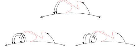
Figure 6. A generalized flower $(F=1,s=+)$ and two possible insertions of an untwisted (1A) and a twisted (1B) petal yielding $(F=1,s=+)$ and $(F=2,s)$, respectively.

(2) We pursue with the configuration $(F=1,s=-)$ described by the unique face which is necessarily of the form given by Figure 7.

(2A) Adding to this flower an untwisted petal, one gets Figure 6 2A, so that $(F=2,s)$.

(2B) Meanwhile, adding to the flower a twisted petal, one ends up with Figure 6 2B, so that $(F=1,s=+)$.

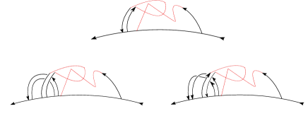
Figure 7. A generalized flower $(F=1,s=-)$ and two possible insertions of an untwisted (2A) and a twisted (2B) petal yielding $(F=2,s)$ and $(F=1,s=+)$, respectively.

(3) Finally, we study the configuration such that $(F=2,s)$ described by two faces with arbitrary orientations of the form given by Figure 8.

(3A) and (3B) Adding to this flower either an untwisted or a twisted petal, the result is given in Figure 6 3A or 3B, respectively. In any situation, one finds $(F=1,s=-)$.

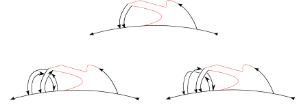
Figure 8. A generalized flower $(F=2,s)$ and two possible insertions of an untwisted (3A) and a twisted (3B) petal yielding the same configuration $(F=1,s=-)$.

Then all relations (14) are satisfied. Hence starting with any configuration of the $N$-petal flower and adding a new petal, either yields $F=1$ or $F=2$. This achieves the proof of Theorem 1.

∎

We have thus obtained the number of faces of the $N$-petal flower with arbitrary number of (twisted or untwisted) petals and without the explicit dependence on the face orientations. Orientations have been used as an artifact of the procedure. However, it is not clear that the number of faces is dependent or not of the cyclic order of the vertex and the fact that we can distinguish two special edges, the first and the final, according to that cyclic order. With commonsensical arguments, one may claim that above number of faces should be the same if we interchange the role of these two edges and reverse the cyclic order of the vertex. We will come back on this point later and prove that this is indeed the case.

Theorem 1 is only useful if an explicit formula for the number of faces of a $N$-petal flower is affordable. It is remarkable that we can map the each configuration on a $\mathbb{Z}_{3}$ generator and (14) can be simply encoded in terms of a rule for these generators. We assign

- $(F=1,s=+)\longrightarrow 2\mod 3$

- $(F=1,s=-)\longrightarrow 1\mod 3$

- $(F=2,s)\longrightarrow 0\mod 3$

Notice that, according to our convention, the bare vertex gets mapped on $1$. Defining for any petal $e$ the symbol $\varepsilon_{e}=-1$ if the petal is untwisted or $\varepsilon_{e}=+1$ if the petal is twisted, the above (14) rules simply translate as

$$x^{\prime}=x\varepsilon_{e}+1\mod 3\,,$$ (15)

where $x$ is $\mathbb{Z}_{3}$ generator corresponding to the couple $(F,s)$ as defined above. For instance, for $x=2$, equivalently $(F=1,s=+)$, calculating $2(+1)+1=3=0$ equivalently describes the addition of a twisted petal to a configuration $(F=1,s=+)$ which yields $(F=2,s)$.

Consider now a $N$-petal flower as the result of branching $N\geq 1$ petals on an initial bare vertex. The bare vertex provides us with an initial condition $x_{0}=1\in\mathbb{Z}_{3}$. Inserting a first petal $e_{1}$ we obtain the class $x_{1}\in\mathbb{Z}_{3}$, $x_{1}=x_{0}\varepsilon_{1}+1$, where, for simplicity, we henceforth denote $\varepsilon_{e_{i}}=\varepsilon_{i}$. Then we iterate the procedure by inserting more petals such that, at the end, the number of faces of the flower is directly obtained after evaluating a nested product

$$(F,s) = [[\dots[[[\varepsilon_{1}+1]\varepsilon_{2}+1]\varepsilon_{3}+1]\dots]\varepsilon_{N-1}+1]\varepsilon_{N}+1\mod 3$$ (16)

$$= 1+\sum_{l=0}^{N-1}\prod_{k=0}^{l}\varepsilon_{N-k}\mod 3\,.$$ (17)

Consider an ordered sequence $e_{1},\dots,e_{l},\dots e_{N}$ of self-loops forming the $N$-petal flower, the subset $E_{l}=\{e_{N},\dots,e_{l}\}$ of the final self-loops (starting from a final edge $e_{N}$ and counting in some cyclic order at the vertex up to $e_{1}$) and the subset $E_{\text{unt};l}\subset E_{l}$ of all its untwisted self-loops, then the class $(F,s)$ (17) can be rewritten as

$$(F,s)=1+\sum_{l=0}^{N-1}(-1)^{|E_{\text{unt},N-l}|}\mod 3\,.$$ (18)

Now we come back on a previous remark and consider the reverse construction of the flower. We start by inserting the last edge $e_{N}$ then $e_{N-1}$ and so on up to $e_{1}$. Thus the class that one obtains is

$$(F^{\prime},s^{\prime}) = [[\dots[[[\varepsilon_{N}+1]\varepsilon_{N-1}+1]\varepsilon_{N-2}+1]\dots]\varepsilon_{2}+1]\varepsilon_{1}+1\mod 3$$ (19)

$$= 1+\sum_{l=1}^{N}\prod_{k=1}^{l}\varepsilon_{k}\mod 3\,.$$ (20)

It is direct to recover

$$(F^{\prime},s^{\prime})=(-1)^{|E_{\text{unt},1}|}(F,s)\mod 3\,.$$ (21)

Hence, $(F,s)=0\Leftrightarrow(F^{\prime},s^{\prime})=0$ from which one infers that $F=2=F^{\prime}$, and otherwise necessarily $F=1=F^{\prime}$.

Let us restrict the formula (18) for particular flowers. Assuming that the flower has only untwisted petals, then, according to our rules, by adding successively petals only the sequence $\dots\to 0\to 1\to 0\to 1\dots$ is possible. Moreover,

$$(F,s) = 1+\sum_{l=0}^{N-1}(-1)^{|E_{N-l}|}\mod 3=1+\sum_{l=0}^{N-1}(-1)^{l+1}\mod 3$$ (22)

$$= \frac{1}{2}(1+(-1)^{N})\mod 3\,.$$ (23)

Thus, if $N$ is even $(F,s)=1\mod 3$ and if $N$ is odd $(F,s)=0\mod 3$. In any situation, we directly identify $F=1+\epsilon(N)$, where $\epsilon(N)=(1-(-1)^{N})/2$.

Assuming that the flower has only twisted petals, then for $N\geq 1$,

$$(F,s)=1+\sum_{l=0}^{N-1}(-1)^{0}\mod 3=(1+N)\mod 3\,.$$ (24)

In this case, we simply write $F=1+\epsilon_{(3)}(N)$.

Note that formula (18) determines the number of faces of more general classes of $N$-petal flowers than the two simplest situations discussed above. For instance, whenever $|E_{\text{unt},N-l}|$ depends only on the number of petals of the subgraph (and not the subgraph itself), we could infer a final formula for the number of faces. The method that we will use in Section 4 might hopefully find an extension this more general situation. Although not carried out in the present work, we hope that this analysis can be applied specifically for “periodic” $N$-petal flowers. These ribbon graphs can be defined as a $\{(N_{1},s_{1}),(N_{2},s_{2}),(N_{3},s_{3}),\dots,(N_{q},s_{q})\}$-petal flowers (with merged sectors) with alternate sequence $(N_{i},s_{i})=(k_{1},\pm)$, $(N_{i+1},s_{i+1})=(k_{2},\mp)$, $i,i+1\in[\![1,q]\!]$, with fixed $k_{1}\geq 1$ and $k_{2}\geq 1$. For any of these flowers, the class $(F,s)$ (hence the number of faces) can be derived.

Let us introduce the following quantity

$$A(\eta,\xi,k)=\sum_{l=\eta}^{\xi}(-1)^{l\,k}\,,$$ (25)

where $\eta=0,1,$ $k\geq 1$ and $\xi\geq\eta$ are all integers.

Assume that $q=2\ell$ is even, $\ell\geq 1$, such that the signs alternate $(s_{1}=-,s_{2}=+,\dots,s_{q-1}=-,s_{q}=+)$, is such a case we have

$$(F,s)=1+A(0,\ell-1,k_{1})\sum_{a=1}^{k_{1}}(-1)^{a}+A(1,\ell,k_{1})k_{2}\mod 3\,.$$ (26)

Now if $k_{1}$ is even,

$$(F,s)=1+\ell k_{2}\mod 3\,.$$ (27)

Otherwise $k_{1}$ is odd and we get

$$(F,s)=1+\frac{((-1)^{\ell}-1)}{2}(1+k_{2})\mod 3\,.$$ (28)

Let us assume that $q=2\ell+1$, $\ell\geq 1$, the sequence $(s_{1}=-,s_{2}=+,\dots,s_{q-1}=+,s_{q}=-)$ yields

$$(F,s)=1+A(0,\ell,k_{1})\sum_{a=1}^{k_{1}}(-1)^{a}+A(1,\ell,k_{1})k_{2}\mod 3\,.$$ (29)

Assuming that $k_{1}$ is even, then

$$(F,s)=1+\ell k_{2}\mod 3\,.$$ (30)

Otherwise if $k_{1}$ is odd, we get

$$(F,s) = 1+(-1)\frac{1-(-1)^{(\ell+1)k_{1}}}{2}+(-1)\frac{1-(-1)^{k_{1}\ell}}{2}k_{2}\mod 3$$ (31)

$$= \frac{(1-(-1)^{\ell})}{2}(1-k_{2})\mod 3\,.$$ (32)

Assume that $q=2\ell$ is even, $\ell\geq 1$, such that the signs alternate $(s_{1}=+,s_{2}=-,\dots,s_{q-1}=+,s_{q}=-)$, then we obtain

$$(F,s)=1+A(0,\ell-1,k_{1})\sum_{a=1}^{k_{1}}(-1)^{a}+A(0,\ell-1,k_{1})k_{2}\mod 3\,.$$ (33)

Now if $k_{1}$ is even,

$$(F,s)=1+\ell k_{2}\mod 3\,.$$ (34)

But if $k_{1}$ is odd, one gets

$$(F,s)=1+\frac{((-1)^{\ell}-1)}{2}(1-k_{2})\mod 3\,.$$ (35)

The last case concerns $q=2\ell+1$, $\ell\geq 1$, for which $(s_{1}=+,s_{2}=-,\dots,s_{q-1}=-,s_{q}=+)$, then we obtain

$$(F,s)=1+A(0,\ell-1,k_{1})\sum_{a=1}^{k_{1}}(-1)^{a}+A(0,\ell,k_{1})k_{2}\mod 3\,.$$ (36)

Setting $k_{1}$ even yields

$$(F,s)=1+(\ell+1)k_{2}\mod 3\,,$$ (37)

whereas assuming that $k_{1}$ is odd gives

$$(F,s)=\frac{1+(-1)^{\ell}}{2}(1+k_{2})\mod 3\,.$$ (38)

The simplest periodic rosettes are defined such that $q=1$, $\ell=0$, and $k_{1}=0$ or $k_{2}=0$ but not at the same time. They have been already treated. The above fomulas are again valid again and we could extend these to $k_{1,2}\geq 0$ $q\geq 1$. Another interesting and simple case is the one determined by $k_{1}=1=k_{2}$. In such a situation, we restrict the above results such that

$(a1):\{(s_{1}=-,\dots,s_{q}=+),q=N=2\ell\}$, $(a2):\{(s_{1}=-,\dots,s_{q}=-),q=N=2\ell+1\}$ and $k_{1}$ odd:

$$(a1)\;\;(F,s)_{-+}=(-1)^{\ell}\mod 3\,\qquad(a2)\;\;(F,s)_{--}=0\mod 3\,,$$ (39)

in any case, $F^{(-)}=1+\epsilon(N)$;

or $(b1):\{(s_{1}=+,\dots,s_{q}=-),q=N=2\ell\}$, $(b2):\{(s_{1}=+,\dots,s_{q}=+),q=N=2\ell+1\}$ and $k_{1}$ odd:

$$(b1)\;\;(F,s)_{+-}=1\mod 3\,,\qquad(b2)\;\;(F,s)_{++}=1+(-1)^{\ell}\mod 3\,,$$ (40)

in any situation the number of faces is always $F^{(+)}=1+\epsilon_{(4)}(N)$, where $\epsilon_{(4)}(\alpha)=1$ if $\alpha\in 4\mathbb{N}+3$ and $\epsilon_{(4)}(\alpha)=0$ elsewhere.

4. Proofs of Theorem 2, Corollary 1 and Corollary 2

We start by proving a useful result on compositions.

Lemma 1 (Number of compositions with $I$ odd integers).

Let $n,P,I$ be some integers, such that $0\leq I\leq P\leq n$, $0\leq d\leq D-1$. The number ${\mathcal{C}}_{n}(P,I)$ of compositions of $n$ in $P$ integers among which $I$ odd integers is given by

$${\mathcal{C}}_{n}(P,I)=\left(\begin{array}[]{c}\frac{n+I}{2}-1\\ P-1\end{array}\right)\,\left(\begin{array}[]{c}P\\ I\end{array}\right),$$ (41)

where the brackets stand for binomial coefficients, $n-I\in 2\mathbb{N}$ (i.e. $n$ and $I$ should share the same parity) and $n\geq 2P$ if $n$ is even and $n\geq 2P-1$ if $n$ is odd.

Proof.

Counting the number of compositions of the integer $n$ made of $P$ integers is well-known as $(^{n-1}_{P-1})$. However we now have to distinguish these compositions depending on how many odd integers they contain.

The easy method to achieve this is to add $+1$ to every odd integer in the composition of $n$. More precisely, let us assume that the number of odd integers is $I$. The initial integer $n$ and $I$ have the same parity. We add $+1$ to the $I$ odd integers thus obtaining a composition of the larger integer $n+I$ in terms of solely even integers, i.e a straightforward composition of the integer $(n+I)/2$. Reversely, starting from a composition of the integer $(n+I)/2$, we multiply it by 2 and subtract $1$ to $I$ arbitrary integers among the list of $P$ integers of the composition. Counting the number of such possibilities, it is convenient to distinguish the cases $n$ even and odd for the sake of clarity. For $n=2m$ even, $I=2f$ is also even with $f$ running from 0 to the integer part of $\frac{P}{2}$ (which is bounded by $m$) and we get:

$${\mathcal{C}}_{n}(P,I) = \Big{|}\Big{\{}(q_{1},..,q_{P})\,|\,q_{l}\in\mathbb{N}\setminus\{0\},\,\sum_{p}q_{p}=2m\;\textrm{and}\;\sum_{p}\epsilon(q_{p})=2f\Big{\}}\Big{|}$$ (42)

$$= \left(\begin{array}[]{c}m+f-1\\ P-1\end{array}\right)\,\left(\begin{array}[]{c}P\\ 2f\end{array}\right).$$ (47)

For $n=2m+1$ odd, $I=2f+1$ is odd and runs from $1$ to $P$ and we get:

$${\mathcal{C}}_{n}(P,I) = \Big{|}\Big{\{}(q_{1},..,q_{P})\,|\,q_{l}\in\mathbb{N}\setminus\{0\},\,\sum_{p}q_{p}=2m+1\;\textrm{and}\;\sum_{p}\epsilon(q_{p})=2f+1\Big{\}}\Big{|}$$ (48)

$$= \left(\begin{array}[]{c}m+f\\ P-1\end{array}\right)\,\left(\begin{array}[]{c}P\\ 2f+1\end{array}\right)\,.$$ (53)

∎

As a proof check of Lemma 1 that summing over all values of $f$ (or equivalently $I$), one recovers the number of compositions $(^{n-1}_{P-1})$ of $n$ in $P$ integers. The appendix provides more details on this development.

The number of compositions of $n$ in $P$ parts which contain $I$ specific integers belonging to the set $D\mathbb{N}+d$, for any $d,D\in\mathbb{N}$, $D\geq 2$, $1\leq d\leq D-1$, is fully addressed in the more elaborate framework of generating functions. We gather all these developments in the appendix from which both ${\mathcal{C}}_{n}(P,I)$ and ${\mathcal{C}}^{t}_{n}(P,I)$ (of Theorem 2) can be simply deduced by applying $D=2,3$ and $d=1,2$, respectively, from Lemma 2.

We can now address the proof of our main theorem.

Proof of Theorem 2.

Since all the rosette graphs (hence flowers) have rank equal to 0, the BR polynomial of any flower $\mathcal{G}_{N}$ (twisted or not) with $N$ intertwined petals reads:

$$R_{\mathcal{G}_{N}}(Y,Z)=\sum_{A\subset\mathcal{G}_{N}}Y^{n(A)}\,Z^{1+n(A)-F(A)}\,,$$ (54)

where $A$ runs over all spanning subgraphs of $\mathcal{G}_{N}$. Such subgraphs can be classified as follows. Erasing some petals, we get subgraphs made of $P$ packets of intertwined petals, each packet $p$ with a number $q_{p}$ of petals, respectively. The total number of petals of the subgraph is equal to its nullity, $n=\sum_{p=1}^{P}q_{p}$, and takes values from 0 (the empty graph with a single vertex) to the initial nullity $N$. It remains to study the number of faces and in each case their number is different.

Let us focus first on the untwisted flower. The number of faces actually depends on the parity of the number of petals of each packet. By Theorem 1, defining an index $\epsilon(q)$ equal to 1 if $q$ is odd and 0 if $q$ is even,

$$\epsilon(q)\equiv\,\frac{1}{2}\big{(}1-(-1)^{q}\big{)},$$ (55)

the number of faces counts the number of odd numbers among the list $(q_{1},..,q_{P})$:

$$F=1+\sum_{p=1}^{P}\epsilon(q_{p})\,.$$ (56)

Putting all these pieces together, we get:

$$R_{\mathcal{G}_{N}}(Y,Z) = \sum_{n=0}^{N}Y^{n}\,\sum_{P=0}^{n}{\mathcal{N}}_{N,n}^{P}\sum_{\sum_{p=1}^{P}q_{p}=n}Z^{n-\sum_{p}\epsilon(q_{p})}$$

$$= \sum_{n=0}^{N}Y^{n}\,\sum_{P=0}^{n}{\mathcal{N}}_{N,n}^{P}\sum_{I=0}^{P}Z^{n-I}\,\Big{|}\Big{\{}(q_{1},..,q_{P})\,|\sum_{p}q_{p}=n\;\textrm{and}\;\sum_{p}\epsilon(q_{p})=I\Big{\}}\Big{|},$$

where ${\mathcal{N}}_{N,n}^{P}$ counts the number of occurrence that a given subgraph made of $P$ packets and missing $N-n$ petals can be obtained from the full graph with $N$ petals. Then $I$ counts the number of odd numbers in the composition $(q_{1},..,q_{P})$ of the integer $n$.

Easy combinatorics allows to compute ${\mathcal{N}}_{N,n}^{P}$. The goal is to put back $(N-n)$ petals between the $P$ packets with the possibility of putting petals on the right or on left of all these packets, but with the constraint that at least one petal between each packet. Forgetting a moment about the extremities (i.e putting 0 petals at the left or right of all packets), one is counting the number of compositions of $(N-n)$ in $(P-1)$ integers. This is given by the binomial coefficient $(^{N-n-1}_{P-2})$. Taking into account all the possibilities, we get:

$${\mathcal{N}}_{N,n}^{P}=\left(\begin{array}[]{c}N-n-1\\ P-2\end{array}\right)+2\left(\begin{array}[]{c}N-n-1\\ P-1\end{array}\right)+\left(\begin{array}[]{c}N-n-1\\ P\end{array}\right)\,=\,\left(\begin{array}[]{c}N-n+1\\ P\end{array}\right)\,.$$ (58)

We finally put the lowest and highest order monomials separate to avoid ambiguities in the definition of the binomial coefficients. The fact that $I\in[\![\epsilon(n),P]\!]$ comes from some parity constraints that should satisfy both $n$ and $I$ in order ${\mathcal{C}}_{n}(P,I)$ to be non vanishing, see Lemma 1. This achieves the proof of (7).

Let us discuss now the case of the twisted flower. The number of faces of the subgraph depends now on the $\mathbb{Z}_{3}$ class corresponding to the $q_{p}$’s. From Theorem 1, it is simple, to determine that

$$F=1+\sum_{p=1}^{P}\epsilon_{(3)}(q_{p})\,,$$ (59)

where $\epsilon_{(3)}(q_{p})=1$ if $q_{p}\in 3\mathbb{N}+2$ otherwise $\epsilon_{(3)}(q_{p})=0$.

Thus, we obtain in similar way than before

$$R_{\mathcal{G}^{t}_{N}}(Y,Z) = \sum_{n=0}^{N}Y^{N}\sum_{P=0}^{n}{\mathcal{N}}^{P}_{N,n}\sum_{\sum_{p}^{P}q_{p}=n}Z^{n-\sum_{p}\epsilon_{(3)}(q_{p})}$$ (60)

$$= \sum_{n=0}^{N}Y^{N}\sum_{P=0}^{n}{\mathcal{N}}^{P}_{N,n}\sum_{I=0}^{P}Z^{n-I}\Big{|}\Big{\{}(q_{1},\dots,q_{P})|\,\sum_{p=1}^{P}q_{p}=n\,\text{and}\,\sum_{p=1}^{P}\epsilon_{(3)}(q_{p})=I\Big{\}}\Big{|}\,,$$ (61)

where ${\mathcal{N}}^{P}_{N,n}$ is exactly the same as previously since the procedure of determining of how many subgraphs with $P$ packets the nullity of which is fixed to $n$ are obtained from the initial graph remains the same. We finally get the formula (8) after extracting the contribution of the lowest and highest nullity subgraphs and notice that $I$ should belongs to $[3-{\rm d}_{n},P]$ after satisfying some constraints for getting non vanishing ${\mathcal{C}}^{t}_{n}(P,I)$, see Lemma 2 in the appendix. This completes the proof of the theorem.

∎

We can now provide some examples of $R_{\mathcal{G}_{N}}$ and $R_{\mathcal{G}^{t}_{N}}$. Invoking Lemma 1 in order to compute the remaining cardinal appearing in (4), we get:

$$R_{\mathcal{G}_{N}}(Y,Z) = 1+Y^{N}Z^{N-\epsilon(N)}$$ (63)

$$+ \sum_{n=1}^{N-1}Y^{n}\,\sum_{P\in[\![1,n]\!]\,\&\,P\leq N-n+1}\left(\begin{array}[]{c}N-n+1\\ P\end{array}\right)\Bigg{\{}$$ (71)

$$\sum_{\frac{n-P}{2}\leq k\leq\min(\frac{n}{2},n-P)}Z^{2k}\,\left(\begin{array}[]{c}n-k-1\\ P-1\end{array}\right)\,\left(\begin{array}[]{c}P\\ n-2k\end{array}\right)\Bigg{\}},$$

where we put the lowest and highest order monomials separate to avoid ambiguities in the definition of the binomial coefficients. $k$ is an integer and it is bounded as given in the formula. We can check this formula explicitly for small values of $N$:

$$R_{\mathcal{G}_{1}}(Y,Z)=Y+1\,,$$ (72)

(73)

$$R_{\mathcal{G}_{2}}(Y,Z)=Y^{2}Z^{2}+2Y+1\,,$$ (74)

(75)

$$R_{\mathcal{G}_{3}}(Y,Z)=Y^{3}Z^{2}+Y^{2}(2Z^{2}+1)+3Y+1\,,$$ (76)

(77)

$$R_{\mathcal{G}_{4}}(Y,Z)=Y^{4}Z^{4}+4Y^{3}Z^{2}+3Y^{2}(Z^{2}+1)+4Y+1\,,$$ (78)

(79)

$$R_{\mathcal{G}_{5}}(Y,Z)=Y^{5}Z^{4}+Y^{4}(3Z^{4}+2Z^{2})+Y^{3}(9Z^{2}+1)+Y^{2}(4Z^{2}+6)+5Y+1\,.$$ (80)

Meanwhile, for $\mathcal{G}^{t}_{N}$, we have

$$R_{\mathcal{G}^{t}_{N}}(Y,Z)=1+Y^{N}Z^{N-\epsilon_{(3)}(N)}+\sum_{n=1}^{N-1}Y^{n}\sum_{P\in[\![1,n]\!]\,\&\,P\leq N-n+1}\left(\begin{array}[]{c}N-n+1\\ P\end{array}\right)\Bigg{\{}$$ (83)

$$\sum_{I=0}^{P}Z^{n-I}\Big{[}\sum_{[l\in[\![0,P-I]\!]]\,\&\,[2l\in M_{3,3-{\rm d}_{n+I}}\text{ or }M_{3,0}]}\left(\begin{array}[]{c}P\\ l,I,P-l-I\end{array}\right)\left(\begin{array}[]{c}\frac{n+I+2l}{3}-1\\ P-1\end{array}\right)\Big{]}\Bigg{\}},$$ (88)

where $n\geq 3P-{\rm d}_{I}$ and the last sum is only nontrivial for terms such that $n+I+2l\geq 3P$. Setting $N=1,2,\dots,5$, we obtain

$$R_{\mathcal{G}^{t}_{1}}(Y,Z)=YZ+1\,,$$ (89)

(90)

$$R_{\mathcal{G}^{t}_{2}}(Y,Z)=Y^{2}Z+2YZ+1\,,$$ (91)

(92)

$$R_{\mathcal{G}^{t}_{3}}(Y,Z)=Y^{3}Z^{3}+Y^{2}(Z^{2}+2Z)+3YZ+1\,,$$ (93)

(94)

$$R_{\mathcal{G}^{t}_{4}}(Y,Z)=Y^{4}Z^{4}+2Y^{3}(Z^{3}+Z^{2})+3Y^{2}(Z^{2}+Z)+4YZ+1\,,$$ (95)

(96)

$$R_{\mathcal{G}^{t}_{5}}(Y,Z)=Y^{5}Z^{4}+Y^{4}(4Z^{4}+Z^{2})+Y^{3}(4Z^{3}+6Z^{2})+Y^{2}(6Z^{2}+4Z)+5YZ+1\,.$$ (97)

Proof of Corollary 1.

This is a direct consequence of the factorization of the BR polynomial in terms of polynomials for product of graphs. We recall first that for a product graph $\mathcal{G}_{1}\cdot\mathcal{G}_{2}$ of two disjoint ribbon graphs $\mathcal{G}_{1}$ and $\mathcal{G}_{2}$ glued along one of their vertex [2], the BR polynomial is given by

$$R_{\mathcal{G}_{1}\cdot\mathcal{G}_{2}}=R_{\mathcal{G}_{1}}\cdot R_{\mathcal{G}_{2}}\,.$$ (98)

Consider now a graph $\mathcal{G}$ having a trivial $N$-petal flower $G_{N}$ subgraph, then it is easy to factor $\mathcal{G}$ as $G_{N}\cdot\mathcal{G}_{\mathcal{G}-G_{N}}$. The statement is therefore obvious from (98). ∎

Proof of Corollary 2.

Using Corollary 1 and previous results on terminal forms as bridges and trivial self-loops, the result becomes immediate. ∎

On a $(1,1)$-periodic $N$-petal flower. Consider the $(k_{1},k_{2})$-periodic $N$-petal flower (according to our discussion in Section 3). The problem of finding an explicit expression for the BR polynomial associated with this graph becomes more involved and should reduce again to a counting of specific compositions.

For a matter of simplicity, let us discuss the case $(k_{1}=1,k_{2}=1)$-periodic $N$-petal flower $\mathcal{G}^{\prime}_{N}$. We again consider an expansion of the polynomial in terms of the nullity. At fixed nullity $n$, we consider $P$ packet subgraphs $(q_{1},\dots,q_{P})$. According to (39) and (40), the number of faces in each packet depends on the quality of the its last petal. It is clear that we can decompose the list $(q_{1},..,q_{P})$ in $(q_{i_{1}},..,q_{i_{l_{1}}})$ for which the last petal of each $i_{p}$ packet is untwisted, and $(q_{j_{1}},..,q_{j_{l_{2}}})$ for which the last petal of each $j_{p}$ packet is twisted. Hence $l_{1}+l_{2}=P$.

The number of faces in the subgraph corresponding to the list $(q_{1},..,q_{P})$ is simply given by

$$F=1+\sum_{p=1}^{l_{1}}\epsilon(q_{i_{p}})+\sum_{p=1}^{l_{2}}\epsilon_{(4)}(q_{j_{p}})\,.$$ (99)

Arguing as above in the above proof of Theorem 2, we see that there is two layers of difficulty when one asks for a closed formula for a polynomial for $\mathcal{G}^{\prime}_{N}$. For a subgraph corresponding to a composition $(q_{1},..,q_{P})$, we need to know which of the packets start by a twisted petal (and so which do not). This leads to consider more general “signed” composition $(q_{1}^{\varepsilon_{1}},q_{2}^{\varepsilon_{2}},\dots,q_{P}^{\varepsilon_{P}})$, where $\varepsilon_{i}=\pm$, determines if the starting petal in the packet $i$ is twisted or not, respectively. Having find a way to encode these signed compositions for any subgraph, and summing on all of these subsets of compositions, then the remaining task is to count again among these compositions those containing $I$ odd integers and $J$ integers in $4\mathbb{N}+3$.

5. Recurrence relations

In fact, there is an alternative way to determine the above BR polynomial of the $N$-petal flower worthwhile to be discussed.

Consider a $N$-petal flower $\mathcal{G}$ and its spanning subgraphs. We can assign an index to each petal, $\{e_{i}\}_{i=1,\dots,N}$ and we can, for instance, label them from the top to the bottom (using the cyclic order). Then, choose $e_{1}$ (or $e_{N}$, without loss of generality). Then the spanning subgraphs of $\mathcal{G}$ can be divided into two sets: a set $S_{e_{1}}$ which contains $e_{1}$ and another $S_{\check{e}_{1}}$ which does not. It is immediate that the polynomial for $\mathcal{G}$ can be written

$$R_{N}=R_{N-1}+R^{\prime}$$ (100)

where $R_{N-1}$ is a BR polynomial for a $(N-1)$-petal flower built from $S_{\check{e}_{1}}$ or spanning subgraphs made with $\{e_{2},e_{3},\dots,e_{N}\}$ and $R^{\prime}$ is a sum of all contributions coming from subgraphs containing $e_{1}$. Among these subgraphs containing $e_{1}$, we can specify subgraphs which do not contain $e_{2}$ and those which do. A moment of thought leads one to the result

$$R^{\prime}=c(Y,Z)R_{N-2}+R^{\prime\prime}$$ (101)

where $c(Y,Z)$ depends on the type of the petal $e_{1}$; if $e_{1}$ is untwisted then $c(Y,Z)=Y$; if $e_{1}$ is twisted then $c(Y,Z)=YZ$. One iterates the procedure until there is no petal left. Finally, adding the empty graph and the total graph contribution, we get a recurrence relation that $R_{N}$ should satisfy:

$$R_{N}(Y,Z)=\sum_{n=0}^{N-1}Y^{n}Z^{n-\epsilon_{(\alpha)}(n)}R_{N-n-1}(Y,Z)+Y^{N}Z^{N-\epsilon_{(\alpha)}(N)}\,,$$ (102)

for all $N\in\mathbb{N}$, $N\geq 1$, and where $\alpha=2,3$ given the particular type of flower we are dealing with: $\epsilon_{(2)}(q)=(1-(-1)^{q})/2$ if we have a untwisted flower and $\epsilon_{(3)}(q)=1$ if $q\in 3\mathbb{N}+2$ otherwise $\epsilon_{(3)}(q)=0$, for the twisted case.

Notice that such a recurrence relation is difficult to solve for arbitrary $N$ by ordinary methods. However, given $\alpha=2,3$, the above techniques show that explicit solutions for such recurrence equations are affordable.

Acknowledgements

Discussions with Vincent Rivasseau are gratefully acknowledged. RCA thanks the Perimeter Institute for its hospitality. Research at Perimeter Institute is supported by the Government of Canada through Industry Canada and by the Province of Ontario through the Ministry of Research and Innovation. This work is partially supported by the Abdus Salam International Centre for Theoretical Physics (ICTP, Trieste, Italy) through the Office of External Activities (OEA)-Prj-15. The ICMPA is also in partnership with the Daniel Iagolnitzer Foundation (DIF), France.

Appendix: On compositions

We address in this appendix important remarks on the number of compositions and number of specific compositions containing a certain number of particular integers. These numbers of compositions have been extensively used in the text.

The number of compositions of the integer $n$ in $P$ integers is the coefficient of $t^{n}$ of the following generating function:

$$\left(\sum_{k=1}^{\infty}t^{k}\right)^{P} = \sum_{n=1}^{\infty}\Big{(}\sum_{k_{1}+k_{2}+\dots+k_{P}=n}1\Big{)}t^{n}$$ (A.1)

$$= t^{P}\frac{1}{(1-t)^{P}}=t^{P}\sum_{k=0}^{\infty}t^{k}\left(\begin{array}[]{c}P+k-1\\ k\end{array}\right)=\sum_{n=P}^{\infty}\left(\begin{array}[]{c}n-1\\ P-1\end{array}\right)t^{n}\,.$$ (A.6)

In order to compute the number of compositions of $n$ in $P$ parts containing a number $I$ of odd integers (or of $P-I$ even integers), we further decompose the above expression as

$$\left(\sum_{k=1}^{\infty}t^{k}\right)^{P}=\sum_{n=1}^{\infty}\sum_{I=0}^{P}\Big{(}\sum_{k_{1}+k_{2}+\dots+k_{P}=n\,\&\,I_{2}(k_{1},k_{2},\dots,k_{P})=I}1\Big{)}t^{n}\,,$$ (A.7)

where $(k_{1},k_{2},\dots,k_{P})$ is a composition of $n$, $I_{2}(k_{1},k_{2},\dots,k_{P})$ is a function calculating the number of odd integers in that composition (respectively, calculating the number of even integers in the composition; in the above sum the condition should change as $I_{2}(k_{1},k_{2},\dots,k_{P})=P-I$). Next, we perform the following transformation:

$$\left(\sum_{k=1}^{\infty}t^{k}\right)^{P} = \sum_{I=0}^{P}\left(\begin{array}[]{c}P\\ I\end{array}\right)\left(\sum_{k\in 2\mathbb{N}+1}^{\infty}t^{k}\right)^{I}\left(\sum_{k\in 2\mathbb{N}+2}t^{k}\right)^{P-I}=\sum_{I=0}^{P}\left(\begin{array}[]{c}P\\ I\end{array}\right)t^{-I}\left(\sum_{k\in 2\mathbb{N}+2}^{\infty}t^{k}\right)^{P}$$ (A.12)

$$= \sum_{I=0}^{P}\left(\begin{array}[]{c}P\\ I\end{array}\right)\sum_{k=0}^{\infty}\left(\begin{array}[]{c}P+k-1\\ P-1\end{array}\right)t^{2(k+P)-I}$$ (A.17)

$$= \sum_{n\in 2\mathbb{N}\,\&\,n\geq 2P}^{\infty}\sum_{I^{\prime}=0}^{[\frac{P}{2}]}\left(\begin{array}[]{c}P\\ 2I^{\prime}\end{array}\right)\left(\begin{array}[]{c}\frac{n+2I^{\prime}}{2}-1\\ P-1\end{array}\right)t^{n}$$ (A.27)

$$+\sum_{n\in 2\mathbb{N}+1\,\&\,n\geq 2P-1}^{\infty}\sum_{I^{\prime}=0}^{[\frac{P}{2}]}\left(\begin{array}[]{c}P\\ 2I^{\prime}+1\end{array}\right)\left(\begin{array}[]{c}\frac{n+2I^{\prime}+1}{2}-1\\ P-1\end{array}\right)t^{n}\,,$$

where we use (A.1) as an intermediate step to compute the sum over even integers. Then, we get

$$n\in 2\mathbb{N}\;\,\text{and}\;\,n\geq 2P\,,\qquad\sum_{I=0\,\&\,I\,\text{even}}^{P}\left(\begin{array}[]{c}P\\ I\end{array}\right)\left(\begin{array}[]{c}\frac{n+I}{2}-1\\ P-1\end{array}\right)=\left(\begin{array}[]{c}n-1\\ P-1\end{array}\right);$$ (A.34)

$$n\in 2\mathbb{N}+1\;\,\text{and}\;\,n\geq 2P-1\,,\qquad\sum_{I=1\,\&\,I\,\text{odd}}^{P}\left(\begin{array}[]{c}P\\ I\end{array}\right)\left(\begin{array}[]{c}\frac{n+I}{2}-1\\ P-1\end{array}\right)=\left(\begin{array}[]{c}n-1\\ P-1\end{array}\right).$$ (A.41)

The number of compositions containing $I$ odd integers is simply given by the summand of the above ${\mathcal{C}}_{n}(P,I)=(^{P}_{I})\big{(}^{(n+I)/2-1}_{P-1}\big{)}$.

It is far advantageous to introduce a generalized version of Lemma 1 valid in any situation.

Lemma 2 (Number of compositions with $I$ integers belonging to $D\mathbb{N}+d$).

Let $n,P,I,D,d$ be some integers, such that $I\leq P\leq n$, $1\leq d\leq D-1$, $D\geq 2$. We denote ${\rm d}_{q}$ the remainder of the Euclidean division of $q\in\mathbb{N}$ by $D$. The number ${\mathcal{C}}^{D,d}_{n,P,I}$ of compositions of $n$ in $P$ parts among which $I$ integers belonging to $D\mathbb{N}+d$ is given by

$${\mathcal{C}}^{D,d}_{n,P,I}=\sum_{[\sum_{\alpha=1\,\&\,\alpha\neq d}^{D}l_{\alpha}=P-I]\,\&\,[\sum_{\alpha=1\,\&\,\alpha\neq d}^{D-1}(D-\alpha)l_{\alpha}\in M_{D,D-{\rm d}_{n+(D-d)I}}\text{ or }M_{D,0}]}\Bigg{\{}$$ (A.42)

$$\left(\begin{array}[]{c}P\\ l_{1},l_{2},\dots,l_{d-1},I,l_{d+1}\dots,l_{D}\end{array}\right)\left(\begin{array}[]{c}\frac{n+(D-d)I+\sum_{\alpha=1\&\alpha\neq d}^{D-1}(D-\alpha)l_{\alpha}}{D}-1\\ P-1\end{array}\right)\Bigg{\}},$$ (A.47)

where the first and the second bracket denote the multinomial and binomial coefficients, respectively.

Proof.

Let $D,d\in\mathbb{N}$, such that $d\leq D$. Consider the set

$$M_{D,d}=\{d,D+d,2D+d,3D+d,\dots,kD+d,\dots\}=D\mathbb{N}+d\subset\mathbb{N}\,.$$ (A.48)

Remark that $M_{0,0}=\{0\}$, $M_{1,0}=\mathbb{N}$, $M_{2,1}$ is the set of odd positive integers and $M_{2,0}$ is the set of even positive integers including 0. In general, $M_{D,0}$ is the set of multiples of $D$ and $\mathbb{N}=\cup_{d=0}^{D-1}M_{D,d}$ if $D\geq 1$.

Let us define the function $I_{D,d}$ on the composition $(k_{1},k_{2},\dots,k_{P})$ of some integer $n$ in $P$ integer parts, such that $I_{D,d}(k_{1},k_{2},\dots,k_{P})$ counts the numbers of elements $k_{i}$ of the composition which belong to $M_{D,d}$. Note that $I_{2,1}$ counts the number of odd integers in the composition, hence the above notation $I_{2}=I_{2,1}$.

Expanding the generating function as

$$\left(\sum_{k=1}^{\infty}t^{k}\right)^{P}=\sum_{n=1}^{\infty}\sum_{I=0}^{P}\Big{(}\sum_{k_{1}+k_{2}+\dots+k_{P}=n\,\&\,I_{D,d}(k_{1},k_{2},\dots,k_{P})=I}1\Big{)}t^{n}\,,$$ (A.49)

for $D\geq 2$, $1\leq d\leq D-1$, we aim at computing the coefficient of $t^{n}$. We use the same technique as before and find, for all $D\geq 2$,

$$\left(\sum_{k=1}^{\infty}t^{k}\right)^{P}=\left(\sum_{k\in M_{D,D}}^{\infty}t^{k}+\sum_{k\in M_{D,D-1}}^{\infty}t^{k}+\dots+\sum_{k\in M_{D,2}}^{\infty}t^{k}+\sum_{k\in M_{D,1}}^{\infty}t^{k}\right)^{P}$$ (A.50)

$$=\sum_{l_{1}+l_{2}+\dots+l_{D}=P}\left(\begin{array}[]{c}P\\ l_{1},l_{2},\dots,l_{D-1},l_{D}\end{array}\right)$$ (A.53)

$$\left(\sum_{k\in M_{D,D}}^{\infty}t^{k}\right)^{l_{D}}\left(\sum_{k\in M_{D,D-1}}^{\infty}t^{k}\right)^{l_{D-1}}\dots\left(\sum_{k\in M_{D,2}}t^{k}\right)^{l_{2}}\left(\sum_{k\in M_{D,1}}^{\infty}t^{k}\right)^{l_{1}},$$ (A.54)

where the first bracket $(^{P}_{l_{1},\dots,l_{D}})$ stands for a multinomial coefficient. Computing further, we obtain

$$\left(\sum_{k=1}^{\infty}t^{k}\right)^{P}=\sum_{l_{1}+l_{2}+\dots+l_{D}=P}\left(\begin{array}[]{c}P\\ l_{1},l_{2},\dots,l_{D-1},l_{D}\end{array}\right)\frac{1}{t^{l_{D-1}+2l_{D-2}+\dots+(D-1)l_{1}}}\left(\sum_{k\in M_{D,D}}^{\infty}t^{k}\right)^{P},$$ (A.55)

and using again (A.1), we write

$$\left(\sum_{k=1}^{\infty}t^{k}\right)^{P}=\sum_{l_{1}+l_{2}+\dots+l_{D}=P}\left(\begin{array}[]{c}P\\ l_{1},l_{2},\dots,l_{D-1},l_{D}\end{array}\right)\frac{1}{t^{\sum_{\alpha=1}^{D-1}(D-\alpha)l_{\alpha}}}\sum_{k=0}^{\infty}\left(\begin{array}[]{c}P+k-1\\ k\end{array}\right)t^{D(k+P)}.$$ (A.56)

We fix $1\leq d\leq D-1$, $l_{d}=I$ and want to perform a change in variable as

$$k\to n=D(k+P)-(D-d)I-\sum_{\alpha=1\,\&\,\alpha\neq d}^{D-1}(D-\alpha)l_{\alpha}\,,$$ (A.57)

this requires that $n+(D-d)I+\sum_{\alpha=1\,\&\,\alpha\neq d}^{D-1}(D-\alpha)l_{\alpha}$ should be a multiple of $D$. Given $q\in M_{D,s}$, we denote ${\rm d}_{q}=s$, therefore (A.57) implies that

- ${\rm d}_{\sum_{\alpha=1\,\&\,\alpha\neq i}^{D-1}(D-\alpha)l_{\alpha}}=D-{\rm d}_{(n+(D-d)I)}<D$ which holds for ${\rm d}_{(n+(D-d)I)}$ non vanishing;

- ${\rm d}_{\sum_{\alpha=1\,\&\,\alpha\neq d}^{D-1}(D-\alpha)l_{\alpha}}=0$ for ${\rm d}_{(n+(D-d)I)}$ vanishing.

One notices that, given $n,D,d$ and $I$, these two circumstances exclude each other. We write these conditions $[\sum_{\alpha=1\,\&\,\alpha\neq d}^{D-1}(D-\alpha)l_{\alpha}\in M_{D,D-{\rm d}_{(n+(D-d)I)}}\text{ or }M_{D,0}]$ but one pays attention that, given $n,D$ and $d$, one has to choose between these.

Now, the change the order of the summations and introduce some constraints in the $l_{\alpha}$, for a given $1\leq d\leq D-1$,

$$\left(\sum_{k=1}^{\infty}t^{k}\right)^{P}=$$ (A.58)

$$=\sum_{k=0}^{\infty}\;\,\,\sum_{I=0}^{P}\,\sum_{\sum_{\alpha=1\,\&\,\alpha\neq d}^{D}l_{\alpha}=P-I}\Bigg{\{}$$ (A.59)

$$\left(\begin{array}[]{c}P\\ l_{1},l_{2},\dots,l_{d-1},I,l_{d+1}\dots,l_{D}\end{array}\right)\left(\begin{array}[]{c}P+k-1\\ P-1\end{array}\right)t^{D(k+P)-(D-d)I-\sum_{\alpha=1\,\&\,\alpha\neq d}^{D-1}(D-\alpha)l_{\alpha}}\Bigg{\}}\,.$$ (A.64)

(A.65)

Hence, changing now variable $k\to n$, $n\geq DP-{\rm d}_{(D-d)I}$, the coefficient of $t^{n}$ in the above sum is given by

$$\sum_{I=0}^{P}\sum_{[\sum_{\alpha=1\,\&\,\alpha\neq d}^{D}l_{\alpha}=P-I]\,\&\,[\sum_{\alpha=1\,\&\,\alpha\neq d}^{D-1}(D-\alpha)l_{\alpha}\in M_{D,D-{\rm d}_{(n+(D-d)I)}|}\text{ or }M_{D,0}]}\Bigg{\{}$$ (A.66)

$$\left(\begin{array}[]{c}P\\ l_{1},l_{2},\dots,l_{d-1},I,l_{d+1}\dots,l_{D}\end{array}\right)\left(\begin{array}[]{c}\frac{n+(D-d)I+\sum_{\alpha=1\&\alpha\neq d}^{D-1}(D-\alpha)l_{\alpha}}{D}-1\\ P-1\end{array}\right)\Bigg{\}}=\left(\begin{array}[]{c}n-1\\ P-1\end{array}\right)\,.$$ (A.73)

We also deduce that the cardinal of

$$\Big{\{}(q_{1},\dots,q_{P})|\;q_{l}\in\mathbb{N}\;,\sum_{l=1}^{P}q_{l}=n\;\text{ and }\;I_{D,d}(q_{1},\dots,q_{P})=I\Big{\}}$$ (A.74)

is nothing but

$${\mathcal{C}}^{D,d}_{n,P,I}=\sum_{[\sum_{\alpha=1\,\&\,\alpha\neq d}^{D}l_{\alpha}=P-I]\,\&\,[\sum_{\alpha=1\,\&\,\alpha\neq d}^{D-1}(D-\alpha)l_{\alpha}\in M_{D,D-{\rm d}_{(n+(D-d)I)}}\text{ or }M_{D,0}]}\Bigg{\{}$$ (A.76)

$$\left(\begin{array}[]{c}P\\ l_{1},l_{2},\dots,l_{d-1},I,l_{d+1}\dots,l_{D}\end{array}\right)\left(\begin{array}[]{c}\frac{n+(D-d)I+\sum_{\alpha=1\&\alpha\neq d}^{D-1}(D-\alpha)l_{\alpha}}{D}-1\\ P-1\end{array}\right)\Bigg{\}}$$ (A.81)

for $n\geq DP-{\rm d}_{(D-d)I}$.

∎

We emphasize that it could happen that the binomial coefficient vanishes. The additional condition for the coefficient to be non vanishing reads off as

$$n+(D-d)I+\sum_{\alpha=1\,\&\,\alpha\neq d}^{D-1}(D-\alpha)l_{\alpha}\geq DP\,.$$ (A.82)

In particular, computing

- the $N$-untwisted-petal flower we need to evaluate ${\mathcal{C}}^{2,1}_{n,P,I}$ (and denoted by ${\mathcal{C}}_{n}(P,I)$ in Theorem 2) that we can deduce from the above formula as, given ${\rm d}_{n}=d$,

$${\mathcal{C}}^{2,1}_{n;P;I}=\left(\begin{array}[]{c}P\\ I,P-I\end{array}\right)\left(\begin{array}[]{c}\frac{n+I}{2}-1\\ P-1\end{array}\right)=\left(\begin{array}[]{c}P\\ I\end{array}\right)\left(\begin{array}[]{c}\frac{n+I}{2}-1\\ P-1\end{array}\right)\,,$$ (A.91)

where $n$ and $I$ should have the same parity and $n\geq 2P-{\rm d}_{I}$;

- the $N$-twisted-petal flower the relevant cardinal is ${\mathcal{C}}^{3,2}_{n,P,I}$ (and denoted by ${\mathcal{C}}^{t}_{n}(P,I)$ in Theorem 2) that we can deduce as, given ${\rm d}_{n}=d$,

$${\mathcal{C}}^{3,2}_{n,P,I} = \sum_{[l_{1}+l_{3}=P-I]\,\&\,[2l_{1}\in M_{3,3-{\rm d}_{(n+I)}}\text{ or }M_{3,0}]}\left(\begin{array}[]{c}P\\ l_{1},I,l_{3}\end{array}\right)\left(\begin{array}[]{c}\frac{n+I+2l_{1}}{3}-1\\ P-1\end{array}\right)$$ (A.96)

$$= \sum_{[l\in[\![0,P-I]\!]]\,\&\,[2l\in M_{3,3-{\rm d}_{(n+I)}}\text{ or }M_{3,0}]}\left(\begin{array}[]{c}P\\ l,I,P-l-I\end{array}\right)\left(\begin{array}[]{c}\frac{n+I+2l}{3}-1\\ P-1\end{array}\right),$$ (A.101)

where $n\geq 3P-{\rm d}_{I}$ and $n+I+2l\geq 3P$.

References

- [1] J. S. Birman, “On the combinatorics of Vassiliev invariants,” Braid groups, knot theory and statistical mechanics II (ed. C. N. Yang and M. L. Ge), Advanced Series in Mathematical Physics 17 (World Scientific, River Edge, NJ, 1994) 1–19.
- [2] B. Bollobas and O. Riordan, “Polynomial of graphs on surfaces,” Math. Ann. 323, 81–96 (2002).
- [3] B. Bollobas and O. M. Riordan, “A polynomial invariant of graphs on orientable surfaces,” Proc. London Math. Soc. 83, 513–531 (2001).
- [4] T. Krajewski, V. Rivasseau, A. Tanasa and Zhituo Wang, “Topological Graph Polynomials and Quantum Field Theory. Part I. Heat Kernel Theories,” Annales Henri Poincare 12, 483 (2011) [arXiv:0811.0186v1 [math-ph]].
- [5] T. Krajewski, V. Rivasseau and F. Vignes-Tourneret, “Topological graph polynomials and quantum field theory. Part II. Mehler kernel theories,” Annales Henri Poincare 12, 483 (2011) [arXiv:0912.5438 [math-ph]].
- [6] W. T. Tutte, “Graph theory,” vol. 21 of Encyclopedia of Mathematics and its Applications (Addison-Wesley, Massachusetts, 1984).