$\phi$ photoprodution with coupled-channel effects

Abstract

We study $\phi$ photoprodution with various hadronic rescattering contributions included, in addition to the Pomeron and pseudoscalar meson-exchange diagrams. We find that the hadronic box diagrams can explain the recent experimental data in the vicinity of the threshold. In particular, the bump-like structure at the photon energy $E_{\gamma}\approx 2.3$ GeV is well explained by the $K\Lambda(1520)$ rescattering amplitude in the intermediate state, which is the dominant contribution among other hadronic contributions. We also find that the hadronic box diagrams are consistent with the observed spin-density matrix elements near the threshold region.

I Introduction

The $\phi(1020)$ meson is distinguished from other vector mesons, since it contains mainly strange quarks. Because of its dominant strange quark content, its decays to lighter mesons and coupling to the nucleon are known to be suppressed by the Okubo-Zweig-Iizuka (OZI) rule. In fact, the strange vector form factors of the nucleon, which is implicitly related to the $\phi$ meson via the vector-meson dominance, is reported to be rather small Ahmed:2011vp . This large $s\bar{s}$ content of the $\phi$ meson makes the meson-exchange picture unfavorable in describing photoproduction of the $\phi$ meson. Thus, the Pomeron Donnachie_etal ; Close_etal is believed to be the main contribution to $\phi$ photoproduction, since it explains the slow rise of the differential cross sections of $\phi$ photoproduction as the energy increases. However, while it is true in the higher energy region, a recent measurement reported by the LEPS collaboration Mibe:2005er shows a bump-like structure around the photon energy $E_{\gamma}\approx 2.3$ GeV. It seems that the Pomeron alone cannot account for this bump-like structure and requires that one should consider other production mechanism of $\phi$ photoproduction near the threshold energy. Moreover, a recent measurement of the spin-density matrix elements near the threshold region Chang:2010dg implies that hadronic degrees of freedom play essential role in the vicinity of the threshold.

So far, the theoretical understanding of the production mechanism for the $\phi$ photoproduction can be summarized as follows:

• General energy-dependence of the cross sections is mainly explained by Pomeron exchange that can be taken as either a scalar meson or a vector meson with charge conjugation $C=+1$. While the Pomeron explains the increase of the differential cross section $d\sigma/dt$ in the forward direction, it cannot describe the behavior of $d\sigma/dt$ near the threshold.

• The exchange of neutral pseudoscalar mesons ($\pi^{0}$, $\eta$) provides a certain contribution to $d\sigma/dt$ near the threshold but it is not enough to explain the threshold behavior of $d\sigma/dt$ Titov:1999eu . Moreover, $\pi^{0}$ and $\eta$ exchanges wrongly predict the spin-density observables and, in particular, $\rho_{1-1}^{1}$ matrix element (see Appendix for its definition).

• Usual vector meson-exchanges such as $\rho$ and $\omega$ are forbidden due to their negative charge conjugations ($C=-1$). Otherwise, the charge conjugation symmetry will be broken.

• Vector meson-exchanges with exotic quantum number such as $I(J^{PC})=1(1^{-+})$ are allowed but those vector mesons are not much known experimentally. Moreover, as for the experimental data from the deuteron target, exchange of isoscalar mesons is more plausible. On the other hand, there is no experimental evidence for isoscalar hybrid-exotic mesons PDG2012 .

• The contribution of scalar mesons such as $\sigma$ and $f_{0}$ are negligibly small for $d\sigma/dt$ Titov:1999eu .

Understanding this present theoretical and experimental situation in $\phi$ photoproduction, Ozaki et al. ozaki2009 proposed a coupled-channel effects based on the $K$-matrix formalism. They considered the $\gamma N\to K\Lambda^{*}(1520)$ and $K\Lambda^{*}\to\phi N$ kernels Nam:2005uq in the coupled-channel formalism in addition to $\gamma N\to\phi N$ and $\phi N\to\phi N$. It is a very plausible idea, since the threshold energy for the $K\Lambda^{*}$ is quite close to that for the bump-like structure ($E_{\gamma}\approx 2.3$ GeV), the $\Lambda^{*}(1520)$ resonance may influence $\phi$ photoproduction. Moreover, the $\gamma p\to K\Lambda^{*}(1520)$ reaction can be regarded as a subreaction for the $\gamma p\to K\overline{K}p$ process together with the $\gamma p\to\phi p$ one in Ref. Nam:2005uq . In addition, a possible nucleon resonance ($J^{P}=1/2^{-}$) with large $s\bar{s}$ content was also taken into account. Interestingly, the coupled-channel effects were shown to be not enough to explain the bump-like structure $E_{\gamma}\approx 2.3$ GeV. On the other hand, the bump-like structure was described by their possible $N^{*}$ resonance and was interpreted as a destructive interference arising from the $N^{*}$ resonance Kiswandhi:2011cq ; Kiswandhi:2010ub .

In the present work, we want to scrutinize in detail the nontrivial hadronic contributions arising from hadronic box diagrams in addition to Pomeron and pseudoscalar meson exchanges. Extending the idea of Ref. ozaki2009 , we consider seven possible box diagrams with intermdiate $\rho N$, $\omega N$, $\sigma N$, $\pi N$, $K\Lambda(1116)$, $K^{*}\Lambda(1116)$, and $K\Lambda(1520)$ states. However, it is quite complicated to compute these box diagrams explicitly, so that we use the Landau-Cutkosky rule Landau:1959fi ; Cutkosky:1960sp , which yields the imaginary part of the box diagrams by its discontinuity across the branch cut. Though their real part may contribute to the transition amplitude, we will show that the imaginary part already illuminates the coupled-channel effects on the production mechanism of $\gamma p\to\phi p$ near the threshold. The parameters such as the coupling constants and cut-off masses of the form factors will be fixed by describing the corresponding processes and by using experimental and empirical data. Yet unknown parameters are varied as compared to the present experimental data. In addition, we tune the strength of the Pomeron amplitude near the threshold region, where the hadronic contribution seems more significant. It is a legitimate procedure, since the Pomeron gets more important as the energy increases. Thus, we determine the threshold parameter in such a way that the Pomeron exchange becomes effective in the higher energy region. We did not consider any $N^{*}$ resonance, since we do not have much information on them above the $\phi N$ threshold PDG2012 . We will show that the coupled-channel effects are indeed essential in explaining the recent LEPS data, which is the different conclusion from Ref. ozaki2009 .

The present paper is organized as follows. In Section II, we explain the basic formalism. We show how to compute the box diagrams mentioned above. In Section III, we present the numerical results such as the energy dependence of the forward cross sections, the angular distributions, and the spin observables. We also discuss how the $K\Lambda^{*}(1520)$ channel can explain the bump-like structure together with the Pomeron exchange tuned. We discuss in detail the spin-density matrix elements for $\phi$-photoproduction. The final Section is devoted to summary and outlook. In the Appendix, we present the definition of the spin-density matrix elements for reference.

II General Formalism

In the present work, we will employ the effective Lagrangian approach in addition to the Pomeron-exchange.

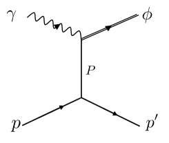
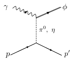
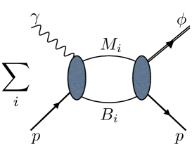
Figure 1: (Color online) Relevant Feynman diagrams for $\phi$ photoproduction: We draw, from the left, the diffractive Pomeron exchange, the pseudoscalar meson-exchanges, and the generic box diagram that includes intermediate meson $M_{i}$ and baryon $B_{i}$ states.

In Fig. 1, we draw the relevant Feynman diagrams which will be involved in describing $\phi$ photoproduction. The first diagram corresponds to the Pomeron-exchange, and the second one depicts $\pi^{0}$- and $\eta$-exchanges. The last diagram represents generically all the contributions from various box diagrams with intermediate hadron states, i.e. $\rho N$, $\omega N$, $\sigma N$, $\pi N$, $K\Lambda(1116)$, $K^{*}\Lambda(1116)$, and $K\Lambda(1520)$, among which the last one was already considered in Ref. ozaki2009 . From now on, we will simply define the $\rho N$ box diagram as that with intermediate $\rho$ and $N$ states, and so on. We also define the 4-momenta of the incoming photon, outgoing $\phi$, the initial (target) proton and the final (recoil) proton as $k_{1}$ and $k_{2}$, $p_{1}$ and $p_{2}$, respectively. In the center of mass (CM) frame, these variables are written as $k_{1}=(k,\bm{k})$, $k_{2}=(E_{\phi},\bm{p})$, $p_{1}=(E_{p},-\bm{k})$ and $p_{2}=(E_{p^{\prime}},-\bm{p})$, where $k=|\bm{k}|$, $E_{\phi}=\sqrt{m_{\phi}^{2}+|\bm{p}|^{2}}$, $E_{p}=\sqrt{m_{p}^{2}+|\bm{k}|^{2}}$, and $E_{p^{\prime}}=\sqrt{m_{p^{\prime}}^{2}+|\bm{p}|^{2}}$, respectively.

II.1 Pomeron exchange

The amplitude of the Pomeron-exchange Donnachie1987 ; Titov:2003bk ; Titov:2007fc is given by

$$\mathcal{M}=-\bar{u}(p_{2})\mathcal{M}_{\mu\nu}u(p_{1})\epsilon_{\phi}^{*\mu}\epsilon_{\gamma}^{\nu},$$ (1)

where $\epsilon_{\phi}$ and $\epsilon_{\gamma}$ are the polarization vectors of the $\phi$ meson and photon. $\mathcal{M}_{\mu\nu}$ is

$$\mathcal{M}^{\mu\nu}=M(s,t)\Gamma^{\mu\nu},$$ (2)

where the transition operator $\Gamma^{\mu\nu}$ is defined as

$$\Gamma^{\mu\nu} = \hbox to0.0pt{/\hss}{k}_{\gamma}\bigg{(}g^{\mu\nu}-\frac{p_{3}^{\mu}p_{3}^{\nu}}{p_{3}^{2}}\bigg{)}-\gamma^{\nu}\bigg{(}k_{\gamma}^{\mu}-p_{3}^{\mu}\frac{k_{1}\cdot p_{3}}{p_{3}^{2}}\bigg{)}$$ (4)

$$-\bigg{(}p_{3}^{\nu}-\bar{p}^{\nu}\frac{k_{\gamma}\cdot p_{3}}{\bar{p}\cdot k_{1}}\bigg{)}\bigg{(}\gamma^{\mu}-\frac{\hbox to0.0pt{/\hss}{p}_{3}p_{3}^{\mu}}{p_{3}^{2}}\bigg{)},$$

with $\bar{p}=(p_{1}+p_{2})/2$. Note that the Pomeron amplitude preserves gauge invariance $k_{1}^{\nu}\mathcal{M}_{\mu\nu}=0$. The corresponding invariant amplitude $M(s,t)$ in Eq.(2) is written as

$$M(s,t)=C_{p}F_{N}(t)F_{\phi}(t)\frac{1}{s}\Big{(}\frac{s-s_{\mathrm{th}}}{4}\Big{)}^{\alpha_{p}(t)}\mathrm{exp}\Big{(}-\frac{i\pi}{2}\alpha_{p}(t)\Big{)},$$ (5)

where $s=(k_{1}+p_{1})^{2}$ and $t=(k_{1}-k_{2})^{2}$. $F_{N}(t)$ is the isoscalar form factor of the nucleon, whereas $F_{\phi}(t)$ is the form factor for the photon-$\phi$ meson-Pomeron vertex. They are parameterized, respectively, as

$$F_{N}(t) = \frac{4M_{N}^{2}-a_{N}^{2}t}{(4M_{N}^{2}-t)(1-t/t_{0})^{2}},$$ (6)

$$F_{\phi}(t) = \frac{2\mu_{0}^{2}}{(1-t/M_{\phi}^{2})(2\mu_{0}^{2}+M_{\phi}^{2}-t)}.$$ (7)

The Pomeron trajectory $\alpha_{p}(p)=1.08+0.25\,t$ in Eq.(5) is determined from hadron elastic scattering in the high-energy region. The prefactor $C_{p}$ in Eq.(5) governs the overall strength of the amplitude and $s_{\mathrm{th}}$ determines the starting energy at which the Pomeron-exchange comes into play. We will discuss the determination of these two parameters in Section III.

II.2 $\pi$- and $\eta$-exchanges

To calculate pseudoscalar meson $(\varphi=\pi^{0},~{}\eta)$ exchange in the $t$ channel, we introduce the following effective Lagrangians:

$$\mathcal{L}_{\phi\gamma\varphi} = \frac{e}{m_{\phi}}g_{\phi\gamma\varphi}\epsilon^{\mu\nu\alpha\beta}\partial_{\mu}\phi_{\nu}\partial_{\alpha}A_{\beta}\varphi~{},$$ (8)

$$\mathcal{L}_{\varphi NN} = \frac{g_{\varphi NN}}{2M_{N}}\bar{N}\gamma_{\mu}\gamma_{5}N\partial^{\mu}\varphi,$$ (9)

where $\phi_{\nu}$, $A_{\beta}$, and $N$ denote the $\phi$ vector meson, photon, and nucleon fields, respectively. $m_{\phi}$ and $M_{N}$ stand for the $\phi$ meson and nucleon masses respectively. $e$ represents the electric charge. The $t$-channel amplitude then takes the following form:

$$\mathcal{M}=\frac{eg_{\varphi NN}g_{\phi\gamma\varphi}}{m_{\phi}}\frac{iF_{\varphi NN}(t)F_{\phi\gamma\varphi}}{t-M_{\varphi}^{2}}\bar{u}(p_{2})(\hbox to0.0pt{/\hss}{k}_{1}-\hbox to0.0pt{/\hss}{k}_{2})\gamma_{5}u(p_{1})\epsilon^{\mu\nu\alpha\beta}k_{2\mu}\epsilon_{\phi\nu}^{*}k_{1\alpha}\epsilon_{\gamma\beta},$$ (10)

where $r$ is the four momentum of an exchanged pseudoscalar meson. We introduce the monopole-type form factors for each vertex $F_{\varphi NN}(t)$ and $F_{\phi\gamma\varphi}$ defined as

$$F_{\varphi NN}(t)\;=\;\frac{\Lambda_{\varphi NN}^{2}-M_{\varphi}^{2}}{\Lambda_{\varphi NN}^{2}-t},\;\;\;F_{\phi\gamma\varphi}(t)\;=\;\frac{\Lambda_{\phi\gamma\varphi}^{2}-M_{\varphi}^{2}}{\Lambda_{\phi\gamma\varphi}^{2}-t}.$$ (11)

The coupling constants and the cutoff masses for the pseudoscalar-exchange, we follow Ref. Titov:1999eu : $g_{\pi NN}=13.26$, $g_{\eta NN}=3.527$ for the $\pi NN$ and $\eta NN$ coupling constants, respectively. The cutoff masses are taken to be $\Lambda_{\pi NN}=0.7\,\mathrm{GeV}$ and $\Lambda_{\eta NN}=1\,\mathrm{GeV}$. Though these values are somewhat different from the phenomenological nucleon-nucleon potentials Machleidt:1989tm ; Rijken:2006en , the effects of the pseudoscalar meson-exchanges on $\phi$ photoproduction are rather small. Thus, we will take the values given above typically used in $\phi$ photoproduction. Those of the coupling constants for the $\phi\gamma\varphi$ vertices are determined by using the radiative decays of the $\phi$ meson to $\pi$ and $\eta$. Using the data from the Particle Data Group (PDG) PDG2012 , one can find $g_{\phi\gamma\pi}=-0.141$ amd $g_{\phi\gamma\eta}=-0.707$. The negative signs of these coupling constants were determined by the phase conventions in SU(3) symmetry as well as by $\pi$ photoproduction Titov:1999eu . We choose the cut-off masses for the $\phi\gamma\pi$ and $\phi\gamma\eta$ form factors as follows: $\Lambda_{\phi\gamma\pi}=0.77$ GeV and $\Lambda_{\phi\gamma\eta}=0.9$ GeV, respectively.

II.3 $K^{+}\Lambda(1520)$ box diagram

In addition to the Pomeron- and pseudoscalar meson-exchanges, we include the seven different box diagrams: $\rho N$, $\omega N$, $\sigma N$, $\pi N$, $K\Lambda(1116)$, $K^{*}\Lambda(1116)$, and $K\Lambda(1520)$. Since the $K\Lambda(1520)$ box diagram is the most significant one among several possibie box diagram in describing $\phi$ photoproduction, we first discuss the $K^{+}\Lambda(1520)$ one and then deal with all other box diagrams in the next subsection. In The $\gamma N\to K^{+}\Lambda(1520)$ process was investigated within an effective Lagrangian method in Ref. Nam:2005uq of which the results were in good agreement with the experimental data. Thus, we will take the formalism developed in Ref.  Nam:2005uq so that we may take into account the $K\Lambda(1116)$ coupled-channel effects more realistically.

The effective Lagrangians for $\gamma N\to K^{+}\Lambda(1520)$ are written as

$$\mathcal{L}_{KN\Lambda^{*}} = \frac{g_{KN\Lambda^{*}}}{M_{K}}\bar{N}\gamma_{5}\partial_{\mu}K^{+}\Lambda^{*\mu},$$ (12)

$$\mathcal{L}_{\phi KN\Lambda^{*}} = -i\frac{g_{KN\Lambda^{*}}}{M_{K}}g_{\phi KK}\bar{N}\gamma_{5}\partial_{\mu}K^{+}\Lambda^{*\mu},$$ (13)

$$\mathcal{L}_{\phi KK} = -ig_{\phi KK}(\partial^{\mu}K^{-}K^{+}-\partial^{\mu}K^{+}K^{-})\phi_{\mu},$$ (14)

$$\mathcal{L}_{\phi NN} = -g_{\phi NN}\bar{N}\left[\gamma_{\mu}\phi^{\mu}-\frac{\kappa_{\phi}}{2M_{N}}\sigma^{\mu\nu}\partial_{\nu}\phi_{\mu}\right]N,$$ (15)

$$\mathcal{L}_{\gamma KK} = -ie(\partial^{\mu}K^{-}K^{+}-\partial^{\mu}K^{+}K^{-})A_{\mu},$$ (16)

$$\mathcal{L}_{\gamma NN} = -e\bar{N}\left[\gamma^{\mu}-\frac{\kappa_{N}}{2M_{N}}\sigma^{\mu\nu}\partial_{\nu}\right]A_{\mu}N,$$ (17)

$$\mathcal{L}_{\gamma KN\Lambda^{*}} = -i\frac{eg_{KN\Lambda^{*}}}{M_{K}}\bar{N}\gamma_{5}\partial_{\mu}K^{+}\Lambda^{*\mu},$$ (18)

where $K$ and $\Lambda^{*\mu}$ denote the $K$ meson and $\Lambda(1520)$ fields. For $\Lambda(1520)$, we utilize the Rarita-Schwinger formalism. $M_{K}$ is the kaon mass. The $KN\Lambda^{*}$ coupling constant is taken from Ref. Nam:2005uq , since we use the amplitude derived in it. The $\phi KK$ coupling constant can be determined from the experimental data for the decay width $\Gamma_{\phi\to KK}$. On the other hand, $g_{\phi NN}$ is not much known experimentally. Recent experiments measuring the strange vector form factors imply that the strange quark gives almost no contribution to the nucleon electromagnetic (EM) form factors Ahmed:2011vp . One can deduce from this experimental fact that the $\phi NN$ coupling constant should be very small. In Ref. Meissner:1997qt , the $\phi NN$ was estimated by using a microscopic hadronic model with $\pi\rho$ continuum: $g_{\phi NN}=\pm 0.25$ and $\kappa_{\phi}=0.2$, which are compatible with the recent data for the strange vector form factors. Thus, we will take these values in the present work. However, note that the $s$-channel contribution with the $\phi NN$ vertex is almost negligible. In Table 1, the relevant strong coupling constants and anomalous magnetic moments are listed.

Table 1: The strong coupling constants and anomalous magnetic moments used in the present work.

$g_{KN\Lambda^{*}}$	11	Ref. Nam:2005uq
$g_{\phi KK}$	4.7	Ref. PDG2012
$g_{\phi NN}$	0.25	Ref. Meissner:1997qt
$\kappa_{p}$	1.79	Ref. PDG2012
$\kappa_{\phi}$	0.2	Ref. Meissner:1997qt

Based on the effective Lagrangians given in Eq.(18), we can write down the amplitude for the $K^{+}\Lambda^{*}(1520)$ box diagram. It contains both real and imaginary parts. The real part is divergent, which is also the case for other box diagrams and the rigorous calculation is rather involved. Thus we consider that the real part can be taken into account effectively by the reenormalization of various coupling constants, and calculate only the imaginary part explicitly. The reasoning behind is similar to the concept of K-matrix formalism for the S-matrix. Physically, the imaginary part corresponds to rescattering and is obtained by the Landau-Cutkosky rule, Ref. Landau:1959fi ; Cutkosky:1960sp .

Having computed the Lorentz-invariant phase space volume factors, we obtain the imaginary part of the amplitude as

$$\mathrm{Im}\mathcal{M}_{K^{+}\Lambda^{*}\mathrm{box}}\;=\;-\frac{1}{8\pi}\frac{r}{\sqrt{s}}\int\frac{d\Omega}{4\pi}\mathcal{M}_{L}(\gamma p\to K^{+}\Lambda^{*})\mathcal{M}_{R}^{\dagger}(K^{+}\Lambda^{*}\to\phi p),$$ (19)

where $r$ is the magnitude of the $K^{+}$ momentum. This imaginary part of the amplitude is schematically drawn in Fig. 2. The shaded ellipse in the left-hand side represents the invariant amplitude for $\gamma p\to K^{+}\Lambda^{*}$, which is basically the same as that of Ref. Nam:2005uq except for different form factors as will be explained later. It consists of three different types of the Feynman diagrams as shown below the left dashed arrow. On the other hand, the right ellipse stands for the $K^{+}\Lambda^{*}\to\phi p$ process that contains the diagrams below the right arrow, generically.

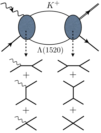
Figure 2: Feynman diagrams for the $K^{+}\Lambda(1520)$ box. The form factors are introduced in a gauge-invariant way.

Note that we use a similar method as in Ref. ozaki2009 but we choose the different form factors and parameters. The corresponding invariant amplitudes $\mathcal{M}_{L}(\gamma p\to K^{+}\Lambda^{*})$ and $\mathcal{M}_{R}(K^{+}\Lambda^{*}\to\phi p)$ with the form factors are defined as follows:

$$\mathcal{M}_{L}(\gamma p\to K^{+}\Lambda^{*}) = (\mathcal{M}_{L,s}+\mathcal{M}_{L,t}+\mathcal{M}_{L,c})F_{L}(s,t),$$ (20)

$$\mathcal{M}_{R}(K^{+}\Lambda^{*}\to\phi p) = (\mathcal{M}_{R,s}+\mathcal{M}_{R,t}+\mathcal{M}_{R,c})F_{R}(s,t),$$ (21)

where $\mathcal{M}_{L,s}$ ($\mathcal{M}_{R,s}$), $\mathcal{M}_{L,t}$ ($\mathcal{M}_{R,t}$), and $\mathcal{M}_{L,c}$ ($\mathcal{M}_{R,c}$) represent the $s$-channel, the $t$-channel, and the contact-term contributions to the $\gamma p\to K^{+}\Lambda^{*}$ ($K^{+}\Lambda^{*}\to\phi p$) process, respectively:

$$\mathcal{M}_{L,s} = \frac{eg_{KN\Lambda^{*}}}{M_{K}}\bar{u}^{\mu}k_{2\mu}\gamma_{5}\frac{\hbox to0.0pt{/\hss}{k}_{1}+\hbox to0.0pt{/\hss}{q}+M_{N}}{q^{2}-M_{N}^{2}}\hbox to0.0pt{/\hss}{\epsilon}u(p_{1}),$$ (23)

$$+\,\frac{e\kappa_{p}g_{KN\Lambda^{*}}}{2M_{N}M_{K}}\bar{u}^{\mu}k_{2\mu}\gamma_{5}\frac{\hbox to0.0pt{/\hss}{q}+M_{N}}{q^{2}-M_{p}^{2}}\hbox to0.0pt{/\hss}{\epsilon}\hbox to0.0pt{/\hss}{k}_{1}u(p_{1}),$$

$$\mathcal{M}_{L,t} = -\frac{2eg_{KN\Lambda^{*}}}{M_{K}}\bar{u}^{\mu}\gamma_{5}u(p_{1})\frac{q_{K}^{\mu}}{t_{K}-M_{K}^{2}},$$ (24)

$$\mathcal{M}_{L,c} = \frac{eg_{KN\Lambda^{*}}}{M_{K}}\bar{u}^{\mu}\epsilon_{\mu}\gamma_{5}u(p_{1}),$$ (25)

$$\mathcal{M}_{R,s} = -i\frac{g_{KN\Lambda^{*}}g_{\phi NN}}{M_{K}}\bar{u}(p_{2})\hbox to0.0pt{/\hss}{\epsilon}_{\phi}^{*}\frac{\hbox to0.0pt{/\hss}{q}+M_{p}}{q^{2}-M_{p}^{2}}\gamma_{5}k_{1}^{\alpha}u^{\alpha}(p_{1}),$$ (27)

$$+\,i\frac{g_{KN\Lambda^{*}}g_{\phi NN}}{M_{K}}\frac{\kappa_{\phi}}{2M_{p}}\bar{u}(p_{2})\hbox to0.0pt{/\hss}{k}_{2}\hbox to0.0pt{/\hss}{\epsilon}_{\phi}^{*}\frac{\hbox to0.0pt{/\hss}{q}+M_{p}}{q^{2}-M_{p}^{2}}\gamma_{5}k_{1}^{\alpha}u^{\alpha}(p_{1}),$$

$$\mathcal{M}_{R,t} = \frac{-ig_{KN\Lambda^{*}}g_{\phi KK}}{M_{K}}\frac{2k_{1}\cdot\epsilon_{\phi}^{*}}{q_{K}^{2}-M_{K}^{2}}\bar{u}(p_{2})\gamma_{5}q_{t}^{\alpha}u^{\alpha}(p_{1}),$$ (28)

$$\mathcal{M}_{R,c} = \frac{-ig_{KN\Lambda^{*}}g_{KNN}}{M_{K}}\bar{u}(p_{2})\gamma_{5}\epsilon_{\phi}^{*\mu}u^{\mu}(p_{1}).$$ (29)

We introduce the form factors $F_{R}(s,t)$ and $F_{L}(s,t)$ for $\mathcal{M}_{R}$ and $\mathcal{M}_{L}$, respectively, in particular, in a gauge-invariant manner for the $\gamma p\to K^{+}\Lambda^{*}$ rescattering:

$$F_{R}(s,t) = \left[\frac{n_{1}\Lambda_{1}^{4}}{n_{1}\Lambda_{1}^{4}+(s-M_{p}^{2})^{2}}\right]^{n_{1}}\left[\frac{n_{2}\Lambda_{2}^{4}}{n_{2}\Lambda_{2}^{4}+t^{2}}\right]^{n_{2}},$$ (30)

$$F_{L}(s,t) = \left[\frac{n_{3}\Lambda_{3}^{4}}{n_{3}\Lambda_{3}^{4}+(s-M_{p}^{2})^{2}}\right]^{n_{3}}\left[\frac{n_{4}\Lambda_{4}^{4}}{n_{4}\Lambda_{4}^{4}+t^{2}}\right]^{n_{4}},$$ (31)

where the cut-off masses $\Lambda_{i}$ and powers $n_{i}$ are fitted to the experimental data for the $\gamma p\to K^{+}\Lambda^{*}$ and $\gamma p\to\phi p$, which are listed in Table 2.

Table 2: Cut-off parameters used in Eq.(30)

$n_{1}$	1
$n_{2}$	1
$n_{3}$	2
$n_{4}$	1
$\Lambda_{1}$	0.8 GeV
$\Lambda_{2}$	0.8 GeV
$\Lambda_{3}$	1.0 GeV
$\Lambda_{4}$	1.0 GeV

In Fig. 3, we draw the numerical result of the total cross section for $\gamma p\to K^{+}\Lambda^{*}$ in comparison with the experimental data taken from Ref. Adelseck1985 . It is in good agreement with the data.

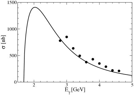
Figure 3: Total cross-section of the $\gamma p\to K\Lambda(1520)$ reaction as compared to the experimental data Adelseck1985 .

II.4 All other box diagrams

In the same manner as done for the $K^{+}\Lambda^{*}$ box diagram, we consider the six intermediate box diagrams as shown in Fig.4, i.e. the $\rho N$, $\omega N$, $\sigma N$, $\pi N$, $K\Lambda(1116)$, and $K^{*}\Lambda(1116)$ box diagrams.

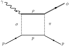
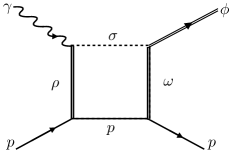
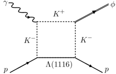
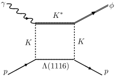
Figure 4: Feynman diagrams for the six hadronic box contributions.

$\rho$ photoproduction has been studied theoretically Friman:1995qm ; Kaneko:2011bd ; Kiswandhi:2011ei ; Kiswandhi:2010ub in which the contributions of the $t$-channel $\pi$- and $\sigma$-exchanges were considered and $\sigma$-exchange was found to be the dominant one, since it selects the isovector part of the EM current. Thus, we take into account the $\rho p$ box diagram with the $\sigma$- and $\pi$-exchanges in the $t$-channel, as shown in the first diagram of Fig. 4. We will show later in Fig. 5 that indeed the $\sigma$-exchange describes qualitatively well the $\gamma p\to\rho p$ reaction. In Ref. Friman:1995qm $\omega$ photoproduction was also discussed within the same framework. In contrast to the $\gamma p\to\rho p$ reaction, the $\pi$-exchange appeared to be dominant, since it picks up the isoscalar part of the EM current. Correspondingly, we consider the $\omega p$ box contribution as in the second diagram of Fig. 4, where $\omega$ is produced by the one pion exchange. The $\sigma p$ and $\pi p$ box diagrams are obtained by reversing the $\rho p$ and $\omega p$ box diagrams. The $\gamma p\to K\Lambda(1116)$ and $\gamma p\to K^{*}\Lambda(1116)$ reactions were measured by several experimental collaborations Glander:2003jw ; Bradford:2005pt ; Sumihama:2005er ; Hicks:2007zz ; Achenbach:2011rf ; Hicks:2010pg and were investigated theoretically Janssen:2001pe ; Oh:2006hm ; Oh:2006in ; Yu:2011fv ; Kim:2011rm . While we consider all the relevant diagrams for the $K\Lambda^{*}(1520)$ box contribution because of its significance, we will take into account only the $K$-exchange diagrams in the $t$-channel for the $K\Lambda$ and $K^{*}\Lambda$ box diagrams, since these two box diagrams turn out to have tiny effects on $\phi$ photoproduction.

The relevant effective Lagrangians for these box diagrams are given as follows:

$$\mathcal{L}_{\gamma\rho\sigma} = \frac{g_{\gamma\rho\sigma}}{m_{\rho}}[\partial_{\mu}A_{\nu}\partial^{\mu}\rho^{\nu}-\partial_{\mu}A_{\nu}\partial^{\nu}\rho^{\mu}]\sigma,$$ (32)

$$\mathcal{L}_{\sigma NN} = g_{\sigma NN}\bar{N}N\sigma,$$ (33)

$$\mathcal{L}_{\pi^{0}NN} = -ig_{\pi NN}\bar{N}\gamma_{5}\tau_{3}N\pi^{0},$$ (34)

$$\mathcal{L}_{\pi\rho\phi} = \frac{g_{\pi\rho\phi}}{m_{\phi}}\epsilon_{\mu\nu\alpha\beta}\partial^{\nu}\phi^{\mu}\partial^{\beta}\rho^{\alpha}\pi_{0},$$ (35)

$$\mathcal{L}_{\omega\phi\sigma} = \frac{g_{\omega\phi\sigma}}{m_{\phi}}(\partial_{\mu}\omega_{\nu}\partial^{\mu}\phi^{\nu}-\partial_{\mu}\omega_{\nu}\partial^{\nu}\phi^{\mu}),$$ (36)

$$\mathcal{L}_{\gamma\omega\pi} = \frac{g_{\gamma\omega\pi}}{m_{\omega}}\epsilon_{\mu\nu\alpha\beta}\partial^{\nu}A^{\mu}\partial^{\beta}\omega^{\alpha}\pi^{0},$$ (37)

$$\mathcal{L}_{VNN} = -g_{VNN}\bar{N}\left(\gamma_{\mu}V^{\mu}-\frac{\kappa_{V}}{2M_{N}}\sigma^{\mu\nu}\partial_{\nu}V_{\mu}\right)N~{},\quad(V=\omega,~{}\rho),$$ (38)

$$\mathcal{L}_{\gamma KK} = -ie\left[(\partial^{\mu}K^{+})K^{-}-(\partial^{\mu}K^{-})K^{+}\right]A_{\mu},$$ (39)

$$\mathcal{L}_{\phi KK} = ig_{\phi KK}\left[(\partial^{\mu}K^{+})K^{-}-(\partial^{\mu}K^{-})K^{+}\right]\phi_{\mu},$$ (40)

$$\mathcal{L}_{KN\Lambda} = -ig_{KP\Lambda}\bar{\Lambda}\gamma_{5}NK^{-},$$ (41)

$$\mathcal{L}_{\gamma KK^{*}} = \frac{g_{\gamma KK^{*}}}{m_{K^{*}}}\epsilon_{\mu\nu\alpha\beta}\partial^{\nu}A^{\mu}\partial^{\beta}K^{*\alpha}K,$$ (42)

$$\mathcal{L}_{\phi KK^{*}} = \frac{g_{\phi KK^{*}}}{m_{\phi}}\epsilon_{\mu\nu\alpha\beta}\partial^{\nu}\phi^{\mu}\partial^{\beta}K^{*\alpha}K,$$ (43)

where the coupling constants and the cut-off masses are listed in Table 3.

Table 3: Coupling constants and cut-off masses used in box diagrams of Fig. 4

$g_{\gamma\rho\sigma}\hskip 28.45274pt$	0.82	Ref.Friman:1995qm
$g_{\sigma NN}$	10.026	Ref.Friman:1995qm
$g_{\pi NN}$	13.26	Ref.Friman:1995qm
$g_{\pi\rho\phi}$	-1.258	Ref.PDG2012
$g_{\phi\omega\sigma}$	-0.45	Ref.PDG2012
$g_{\gamma\omega\pi}$	0.557	Ref.PDG2012
$g_{\omega NN}$	10.35	Ref.titov2002
$g_{\rho NN}$	$3.72$	Ref.titov2002
$g_{\phi KK}$	4.48	Ref.PDG2012
$g_{KN\Lambda}$	-13.26	Ref.nakayama2006
$g_{\gamma KK^{*}}$	0.254 GeV-1	Ref.PDG2012
$g_{\phi KK^{*}}$	10.74	Ref.PDG2012 ; Titov:2004xf
$\kappa_{\omega}$	0	Ref.titov2002
$\kappa_{\rho}$	6.1	Ref.titovKampfer2002
$\Lambda_{\pi\rho\phi}$	1.05 GeV	Ref.Titov:2007fc
$\Lambda_{\pi NN}$	1.05 GeV	Ref.Titov:2007fc
$\Lambda_{\gamma\rho\sigma}$	1.05 GeV	Ref.Friman:1995qm
$\Lambda_{\sigma NN}$	1.1 GeV	Ref.Friman:1995qm
$\Lambda_{\sigma}$	1 GeV	Ref.Friman:1995qm
$\Lambda_{\sigma\rho\rho}$	0.9 GeV	Ref.Friman:1995qm
$\Lambda_{\sigma\omega\phi}$	0.9 GeV	Ref.PDG2012
$\Lambda_{\pi\gamma\omega}$	0.6 GeV	Ref.titov2002
$\Lambda_{V}$	1.227 GeV	Ref.sato1996
$\Lambda_{K}$	1 GeV

The invariant amplitudes for these box diagrams are derived as follows:

$$\mathcal{M}_{1,L} = \frac{g_{\gamma\rho\sigma}g_{\sigma NN}}{M_{\rho}(t_{\sigma}-M_{\sigma}^{2})}\left[(k_{1}\cdot r)(\epsilon_{\gamma}\cdot\epsilon_{\rho}^{*})-(k_{1}\cdot\epsilon_{\rho}^{*})(\epsilon_{\gamma}\cdot r)\right]\bar{u}(q)u(p_{1})\bigg{\{}\frac{\Lambda_{\gamma\rho\sigma}^{2}-M_{\sigma}^{2}}{t_{\sigma}-M_{\sigma}^{2}}\cdot\frac{\Lambda_{\sigma NN}^{2}-M_{\sigma}^{2}}{t_{\sigma}-M_{\sigma}^{2}}\bigg{\}},$$ (44)

$$\mathcal{M}_{1,R} = \frac{-ig_{\phi\rho\pi}g_{\pi NN}}{M_{\phi}(t_{\pi}-M_{\pi}^{2})}\epsilon_{\mu\nu\alpha\beta}\epsilon_{\phi}^{*\mu}k_{2}^{\nu}\epsilon_{\rho}^{\alpha}r^{\beta}\bar{u}(p_{2})\gamma_{5}u(q)\times\bigg{\{}\frac{\Lambda_{\phi\rho\pi}^{2}-M_{\pi}^{2}}{t_{\pi}-M_{\pi}^{2}}\cdot\frac{\Lambda_{\pi NN}^{2}-M_{\sigma}^{2}}{t_{\pi}-M_{\pi}^{2}}\bigg{\}},$$ (45)

$$\mathcal{M}_{2,L} = \frac{-ig_{\gamma\omega\pi}g_{\pi NN}}{M_{\omega}(t_{\pi}-M_{\pi}^{2})}\epsilon_{\mu\nu\alpha\beta}\epsilon_{\gamma}^{\mu}k_{1}^{\nu}\epsilon_{\omega}^{*\alpha}r^{\beta}\bar{u}(q)\gamma_{5}u(p_{1})\times\left\{\frac{\Lambda_{\gamma\omega\pi}^{2}-M_{\pi}^{2}}{t_{\pi}-M_{\pi}^{2}}\cdot\frac{\Lambda_{\pi NN}^{2}-M_{\pi}^{2}}{t_{\pi}-M_{\pi}^{2}}\right\},$$ (46)

$$\mathcal{M}_{2,R} = \frac{-ig_{\phi\omega\sigma}g_{\sigma NN}}{M_{\phi}(t_{\sigma}-M_{\sigma}^{2})}\bar{u}(p_{2})u(q)\big{[}(r\cdot k_{2})(\epsilon_{\omega}\cdot\epsilon_{\phi}^{*})-(r\cdot\epsilon_{\phi}^{*})(k_{2}\cdot\epsilon_{\omega})\big{]}$$ (48)

$$\times\left\{\frac{\Lambda_{\phi\omega\sigma}^{2}-M_{\sigma}^{2}}{t_{\sigma}-M_{\sigma}^{2}}\cdot\frac{\Lambda_{\sigma NN}^{2}-M_{\sigma}^{2}}{t_{\sigma}-M_{\sigma}^{2}}\right\},$$

$$\mathcal{M}_{3,L} = \frac{g_{\rho NN}g_{\gamma\rho\sigma}}{M_{\rho}(t_{\rho}-M_{\rho}^{2})}\Big{[}k_{1}^{\alpha}(\epsilon_{\gamma}\cdot r)-\epsilon_{\gamma}^{\alpha}(k_{1}\cdot r)\Big{]}\bar{u}(p_{2})\bigg{[}\gamma_{\alpha}(1+\kappa_{\rho})-\frac{\kappa_{\rho}}{M_{p}}q^{\alpha}\bigg{]}u(p_{1})$$ (50)

$$\times\Bigg{\{}\Bigg{(}\frac{\Lambda_{\rho}^{2}}{\Lambda_{\rho}^{2}-(\bm{k}_{1}-\bm{r})^{2}}\Bigg{)}^{2}\Bigg{\}},$$

$$\mathcal{M}_{3,R} = \frac{g_{\omega NN}g_{\phi\omega\sigma}}{M_{\phi}(t_{\omega}-M_{\omega}^{2})}\Big{[}(r\cdot\epsilon_{\phi}^{*})k_{2}^{\mu}-(r\cdot k_{2}-M_{\phi}^{2})\epsilon_{\phi}^{*\mu}\Big{]}$$ (52)

$$\times\bar{u}(p_{1})\bigg{[}\gamma_{\mu}(1+\kappa_{\omega})-\frac{\kappa_{\omega}}{2M_{p}}q_{\mu}\bigg{]}u(q)\Bigg{\{}\Bigg{(}\frac{\Lambda_{\omega}^{2}}{\Lambda_{\omega}^{2}-(\bm{r}-\bm{k}_{2})^{2}}\Bigg{)}^{2}\Bigg{\}},$$

$$\mathcal{M}_{4,L} = \frac{-g_{\omega NN}g_{\gamma\omega\pi}}{M_{\omega}(t_{\omega}-M_{\omega}^{2})}\epsilon_{\mu\nu\alpha\beta}\epsilon_{\gamma}^{\mu}k_{1}^{\nu}r^{\beta}\bar{u}(q)\left[\gamma^{\alpha}(1+\kappa_{\omega})-\frac{\kappa_{\omega}}{M_{P}}q^{\alpha}\right]u(p_{1})$$ (54)

$$\times\Bigg{\{}\Bigg{(}\frac{\Lambda_{\omega}^{2}}{\Lambda_{\omega}^{2}-(\bm{r}-\bm{k}_{2})^{2}}\Bigg{)}^{2}\Bigg{\}},$$

$$\mathcal{M}_{4,R} = \frac{-g_{\rho NN}g_{\phi\rho\pi}}{M_{\phi}(t_{\rho}-M_{\rho}^{2})}\epsilon_{\mu\nu\alpha\beta}\epsilon_{\phi}^{*\mu}k_{2}^{\nu}r^{\beta}\bar{u}(p_{2})\left[\gamma^{\alpha}(1+\kappa_{\rho})-\frac{\kappa_{\rho}}{M_{N}}ql^{\alpha}\right]u(q),$$ (56)

$$\times\Bigg{\{}\Bigg{(}\frac{\Lambda_{\rho}^{2}}{\Lambda_{\rho}^{2}-(\bm{k}_{1}-\bm{r})^{2}}\Bigg{)}^{2}\Bigg{\}},$$

$$\mathcal{M}_{5,L} = \frac{-2ieg_{KP\Lambda}}{(t_{L}-M_{K}^{2})}(r\cdot\epsilon_{\gamma})\bar{u}(q)\gamma_{5}u(p_{1})\times\bigg{\{}\left(\frac{\Lambda_{K}^{2}-M_{K}^{2}}{t_{K}-M_{K}^{2}}\right)^{2}\bigg{\}},$$ (57)

$$\mathcal{M}_{5,R} = \frac{2ig_{\phi KK}g_{KP\Lambda}}{(t_{R}^{2}-M_{K}^{2})}(r\cdot\epsilon_{\phi}^{*})\bar{u}(p_{2})\gamma_{5}u(q)\times\bigg{\{}\left(\frac{\Lambda_{K}^{2}-M_{K}^{2}}{t_{K}-M_{K}^{2}}\right)^{2}\bigg{\}},$$ (58)

$$\mathcal{M}_{6,L} = \frac{-ig_{\gamma KK^{*}}g_{KP\Lambda}}{M_{K^{*}}(t_{L}-M_{K}^{2})}\epsilon_{\mu\nu\alpha\beta}\epsilon_{\gamma\mu}k_{1}^{\nu}\epsilon_{K^{*}}^{\alpha}r^{\beta}\bar{u}(q)\gamma_{5}u(p_{1})\times\bigg{\{}\left(\frac{\Lambda_{K}^{2}-M_{K}^{2}}{\Lambda_{K}^{2}-t_{K}}\right)^{2}\bigg{\}},$$ (59)

$$\mathcal{M}_{6,R} = \frac{ig_{\phi KK^{*}}g_{KP\Lambda}}{M_{\phi}(t_{R}-M_{K}^{2})}\epsilon_{\mu\nu\alpha\beta}\epsilon_{\phi}^{*\mu}k_{2}^{\nu}\epsilon_{K^{*}}^{\alpha}r^{\beta}\bar{u}(p_{2})\gamma_{5}u(q)\times\bigg{\{}\left(\frac{\Lambda_{K}^{2}-M_{K}^{2}}{\Lambda_{K}^{2}-t_{K}}\right)^{2}\bigg{\}},$$ (60)

where the subscripts $1,\cdots 6$ correspond to the box diagrams appearing in Fig. 4 in order. The other subscripts $L$ and $R$ denote the $\gamma p\to MB$ and $MB\to\phi p$ parts, respectively. In Figs. 5 and 6 we draw the results of the total cross sections for the $\gamma p\to\rho p$ and $\gamma p\to\omega p$ reactions, respectively. The results are qualitatively in agreement with the experimental data.

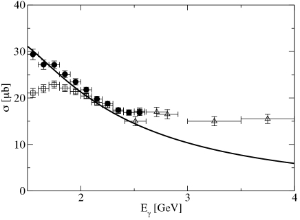
Figure 5: Total cross-section of the $\gamma p\to\rho^{0}p$ reaction. The solid curve depicts the present result obtained from the $t$-channel $\sigma$-exchange diagram. The closed circles and the open squares are taken from Ref. Wu:2005wf , where as the open triangles represent those from Ref. ABBHHM:1968aa .

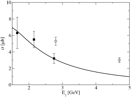
Figure 6: Total cross-section of the $\gamma p\to\omega p$ reaction. The solid curve depicts the present result obtained from the $t$-channel $\pi$-exchange diagram. The closed squares denote the experimental data from Ref. Ballam1973 whereas the open circles represent those from Ref. BHMITPWBubbleChamberGroup:1967zz .

III Numerical results and discussion

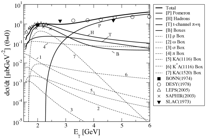
Figure 7: Differential cross section as a function of the photon energy $E_{\gamma}$. The thick solid curve depicts the result with all contributions included. The solid curves with the symbols $P$, $T$, $B$ and $H$ represent the Pomeron contribution, those of $\pi$- and $\eta$-exchanges, those of all the box diagrams, and the total contribution of hadronic diagrams ($T+B$), respectively. The dashed curves with numbers in order denote the effects of the seven box diagrams separately.

We are now in a position to discuss the numerical results for $\phi$ photoproduction. We start with the differential cross section at the forward angle $d\sigma/dt(\theta=0)$ as a function of the photon energy $E_{\gamma}$ in the laboratory frame. The parameters are determined in the following manner. Since the the Pomeron-exchange in the low-energy region is not much understood, we fit the parameter for the overall strength $C_{p}$ and that for the threshold $s_{\mathrm{th}}$ in Eq.(5) in such a way that the Pomeron-exchange reproduces the high energy behavior of the differential cross section: $C_{p}=8\,\mathrm{GeV}^{-1}$ and $s_{\mathrm{th}}=3.83\,\mathrm{GeV}^{2}$. On the other hand, We fix the cut-off parameters for the $K\Lambda^{*}(1520)$ box diagrams to describe the $E_{\gamma}$ dependence of $d\sigma/dt$ in lower energy region, in particular, to explain the well-known bum-like structure around $E_{\gamma}\approx 2.3$ GeV. The parameters of all other hadronic diagrams are taken from existing references as explained in the previous section.

Figure 7 illustrates various contributions to $d\sigma/dt(\theta=0)$ as a function of the photon energy $E_{\gamma}$ from the Pomeron-exchange, the $t$-channel $\pi$- and $\eta$ exchanges, and seven box diagrams. The solid curve with symbol $P$ draws the contribution of the the Pomeron-exchange to $d\sigma/dt$. As expected, it governs $E_{\gamma}$ dependence in the higher energy region ($E_{\gamma}\geq 3$GeV). Note, however, that the Pomeron does not contribute to $d\sigma/dt$ below around $E_{\gamma}=2.3\,\mathrm{GeV}$ in the present work. The $\pi$- and $\eta$-exchanges provide a certain amount of effects on the differential cross section (solid curve with symbol $T$). The contribution of the $\pi$- and $\eta$-exchanges start to increase from the threshold energy and then it decreases very slowly when it reaches approximately 3 GeV. Thus, the effects of the $\pi$- and $\eta$-exchanges are quite important in the lower $E_{\gamma}$ energy region up to $3$ GeV, where the Pomeron-exchange overtakes the $\pi$- and $\eta$-exchanges.

Except for the $K\Lambda^{*}(1520)$ box diagram, all other box contributions turn out to be negligibly small. However, the $K\Lambda^{*}(1520)$ box diagram plays an essential role in describing the experimental data for $d\sigma/dt$ in the lower $E_{\gamma}$ region, in particular, in explaining the bump-like structure near $2.3$ GeV. This is very different from the conclusion of Ref. ozaki2009 , where the $K\Lambda^{*}(1520)$ seems to be suppressed in the $K$-matrix formalism. The reason lies in the fact that we have introduced different form factors for the $\gamma p\to K\Lambda^{*}$ and $K\Lambda^{*}\to\phi p$ reactions. In general, form factors are given as functions of two Mandelstam variables for the box diagrams, i.e. $F(s,\,t)$, since we have two off-shell particles in the $s$-channel and other two off-shell particles in the $t$-channel. However, it is very difficult to preserve the gauge invariance in the presence of the form factors. Thus, we have introduced a type of overall form factors to keep the gauge invariance in the $\gamma p\to K\Lambda^{*}$ part, as written in Eq.(30). To keep the consistency, we also have included a similar type of the form factors in the $K\Lambda^{*}\to\phi p$ part. With these form factors considered, we find that the $K\Lambda^{*}$ box diagram is indeed enhanced as shown in Fig. 7 in comparision with Ref. ozaki2009 . The contribution of the $K\Lambda^{*}$ box diagram increases sharply up to $E_{\gamma}\approx 2$ GeV and then falls off linearly. The result of the $K\Lambda^{*}$ box diagram indicates that the off-shell effects, which arise from the form factors and the rescattering equation, may come into play.

Considering the fact that the $K^{*}\Lambda$ threshold energy ($E_{\mathrm{th}}\approx 2$ GeV) is very close to that of $\phi$ photoproduction ($E_{\mathrm{th}}\approx 1.96$ GeV), one might ask why the contribution of the $K^{*}\Lambda$ is suppressed. While the $K\Lambda^{*}(1520)$ channel ($E_{\mathrm{th}}\approx 2$ GeV) is directly related to $\phi p$, since both are the subreactions of the $\gamma p\to K\bar{K}p$ process, the $\gamma p\to K^{*}\Lambda$ reaction is distinguished from those two reactions, because the $K^{*}\Lambda$ channel is related to $\gamma p\to\pi K\Lambda$ reaction. Thus, one can qualitatively understand why the contribution of the $K^{*}\Lambda$ box diagrams is suppressed.

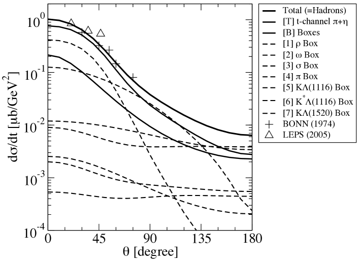
Figure 8: The differential cross section as a function of the scattering angle $\theta$ with the photon energy at $E_{\mathrm{\gamma}}=2$ GeV. The thick solid curve depicts the result with all hadronic contributions included. The solid curves with the symbols $T$ and $B$ represent the contribution of the $\pi$- and $\eta$-exchanges and those of all the box diagrams, respectively. The dashed curves with numbers in order denote the effects of the seven box diagrams separately.

In Fig. 8, the differential cross section as a function of the scattering angle is depicted at $E_{\gamma}=2$ GeV. Since the Pomeron-exchange is suppressed at this photon energy because of $s_{\mathrm{th}}=2.3$ GeV, we can examine each hadronic contribution to the differential cross section more in detail. Figure  8 clearly shows that the $K\Lambda(1520)$ box diagram is the most dominant one among the hadronic contributions. Adding all the effects of the box diagrams, we find that the box contributions almost describe the $\theta$ dependence. Together with the $\pi$- and $\eta$-exchanges, the result of the differential cross section is in good agreement with the experimental data Mibe:2005er ; BESCH:1974aa .

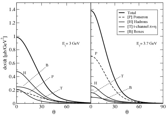
Figure 9: The differential cross section as a function of the scattering angle $\theta$ with two different photon energies $E_{\mathrm{\gamma}}=3$ GeV and $3.7$ GeV. The thick solid curve depicts the result with all contributions included. The solid curves with the symbols $P$, $T$, $B$ and $H$ represent the Pomeron contribution, those of $\pi$- and $\eta$-exchanges, those of all the box diagrams, and the total contribution of hadronic diagrams ($T+B$), respectively.

The differential cross section as a function the scattering angle are drawn in Fig. 9. The left and right panels correspond to the photon energies $E_{\mathrm{\gamma}}=3$ and $3.7$ GeV, respectively. As expected, the hadronic contribution is dominant over the Pomeron-exchange at the lower photon energy, while at $E_{\gamma}=3.7$ GeV, the Pomeron governs the $\gamma p\to\phi p$ process. Interestingly, the effects of the box diagrams, in particular, the $K\Lambda^{*}(1520)$ one, turn out to be larger than those of the $\pi$- and $\eta$-exchanges, whereas the box diagrams seem to be suppressed at higher photon energies. It implies that the $K\Lambda^{*}(1520)$ box diagram influences $\phi$ photoproduction only in the vicinity of the threshold energy.

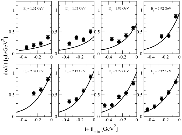
Figure 10: Differential cross sections of the $\gamma p\to\phi p$ reaction as a function of $t+|t|_{\mathrm{min}}$ with eight different photon energies. The experimental data are taken from Ref. Mibe:2005er .

Figure 10 depicts the results of the differential cross section as a function of $t+|t|_{\mathrm{min}}$ with eight different photon energies, where $|t|_{\mathrm{min}}$ is the minimum 4-momentum transfer from the incident photon to the $\phi$ meson. The results are in good agreement with the experimental data taken from the measurement of the LEPS collaboration Mibe:2005er .

It is of great importance to examine the angular distribution of the $\phi\to K^{+}K^{-}$ decay in the $\phi$ rest frame or in the Gottfried-Jackson (GJ) frame, since it makes the helicity amplitudes accessible to experimental investigation Gottfried:1964nx ; Schilling:1969um . The detailed formalism for the angular distribution of the $\phi$ meson decay can be found in Refs. Schilling:1969um ; Titov:1999eu . The decay angular distribution of $\phi$ photoproduction was measured at SAPHIR/ELSA Barth:2003bq but the range of the photon energy is too wide. On the other hand, the LEPS collaboration measured the decay angular distribution at forward angles ($-0.2<t+|t|_{\mathrm{min}}$) in two different energy regions: $1.97<E_{\gamma}<2.17$ GeV and $2.17<E_{\gamma}<2.37$ GeV Mibe:2005er , which are related to the energy around the local maximum of the cross section and that above the local maximum, respectively. Therefore, we have computed the decay angular distributions at two photon energies, i.e. $E_{\gamma}=2.07$ GeV and $E_{\gamma}=2.27$ GeV, which correspond to the center values of the given ranges of $E_{\gamma}$ in the LEPS experiment.

The one-dimensional decay angular distributions $W(\cos\theta)$, $W(\phi-\Phi)$, $W(\phi)$ are presented in Fig. 11, which are expressed respectivley as

$$W(\cos\theta) = \frac{1}{2}(1-\rho^{0}_{00})+\frac{1}{2}\left(3\rho^{0}_{00}-1\right)\cos^{2}\theta,$$ (61)

$$2\pi W(\phi-\Phi) = 1+2p_{\gamma}\overline{\rho}^{1}_{1-1}\cos 2(\phi-\Phi),$$ (62)

$$2\pi W(\phi) = 1-2\mathrm{Re}\rho^{0}_{1-1}\cos 2\phi,$$ (63)

$$2\pi W(\phi+\Phi) = 1+2p_{\gamma}\Delta_{1-1}\cos 2(\phi+\Phi),$$ (64)

$$2\pi W(\Phi) = 1+2p_{\gamma}\rho^{\prime}\cos 2\Phi,$$ (65)

where $\theta$ and $\phi$ denote the polar and azimuthal angles of the decay particle $K^{+}$ in the GJ frame. $\Phi$ represents the azimuthal angle of the photon polarization in the center-of-mass frame. $P_{\gamma}$ stands for the degree of polarization of the photon beam. $\overline{\rho}^{1}_{1-1}$, $\Delta_{1-1}$, and $\rho^{\prime}$ are defined as

$$\overline{\rho}^{1}_{1-1} = \frac{1}{2}(\rho^{1}_{1-1}-\mathrm{Im}\rho^{2}_{1-1}),$$ (66)

$$\Delta_{1-1} = \frac{1}{2}(\rho^{1}_{1-1}+\mathrm{Im}\rho^{2}_{1-1}),$$ (67)

$$\rho^{\prime} = 2\rho^{1}_{11}+\rho^{1}_{00}.$$ (68)

The expressions for the spin-density matrix elements $\rho_{\lambda\lambda^{\prime}}^{\alpha}$ with the helicities $\lambda$ and $\lambda^{\prime}$ for the $\phi$ meson can be found in Appendix A .

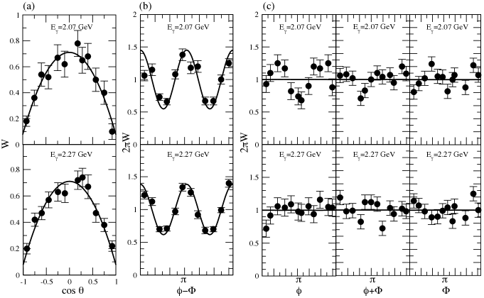
Figure 11: The decay angular distributions for $-0.2<t+|t|_{\mathrm{min}}$ in the Gottfried-Jackson frame. We take the center values of the energy ranges measured by the LEPS collaboration Mibe:2005er , i.e. $E_{\gamma}=2.07$ GeV and $E_{\gamma}=2.27$ GeV. The experimental data are taken from Ref. Mibe:2005er .

The panel (a) of Fig. 11 draws the one-dimensional decay polar-angle distributions $W(\cos\theta)$. As pointed out by Refs. Mibe:2005er ; Chang:2010dg , the decay distribution behaves approximately as $\sim(3/4)\sin^{2}\Psi$, which indicates that the helicity-conserving processes are dominant as shown in Eq.(61). It means that $t$-exchange particles with unnatural parity at the tree level do not contribute to $W(\cos\theta)$. As will be discussed later, $\rho_{00}^{0}$ from the $\pi$- and $\eta$-exchanges, which is related to the single spin-flip amplitude in the GJ frame, exactly vanishes. On the other hand, all hadronic box diagrams contribute to it. Though the Pomeron-exchange might contribute to this spin-density matrix element, it does not play any role below 2.3 GeV. The panel (b) of Fig. 11 shows the results of $W(\phi-\Phi)$, which are in good agreement with the LEPS data, whereas the panel (c) depicts those of $W(\phi)$, $W(\phi+\Phi)$, and $W(\Phi)$, respectively, which deviate from the data. In fact, the data show somewhat irregular behavior which does not seem to be easily reproduced.

Table 4: $\phi$ density matrix in the forward scattering at $E_{\mathrm{\gamma}}=2$ GeV

	$\rho^{0}_{00}$	$\overline{\rho}^{1}_{1-1}$	$\mathrm{Re}\rho^{0}_{1-1}$	$\Delta_{1-1}$	$\rho^{\prime}$
$t$-channel $\pi^{0}+\eta$	0	-0.5	0	0	0
$\rho$ box	$0.651$	$-0.175$	$2.97\times 10^{-4}$	$-8.94\times 10^{-6}$	$1.37\times 10^{-2}$
$\omega$ box	$0.035$	$-0.48$	$9.26\times 10^{-4}$	$-8.72\times 10^{-7}$	$-1.05\times 10^{-3}$
$\sigma$ box	$0.254$	$-0.066$	$-8.85\times 10^{-3}$	$2.03\times 10^{-4}$	$-7.93\times 10^{-4}$
$\pi$ box	$0.061$	$0.448$	$5.57\times 10^{-4}$	$1.79\times 10^{-4}$	$1.15\times 10^{-3}$
$K\Lambda(1116)$ box	$0.025$	$0.488$	$-1.08\times 10^{-2}$	$7.85\times 10^{-5}$	$-2.21\times 10^{-2}$
$K^{*}\Lambda(1116)$ box	$0.030$	$0.485$	$1.39\times 10^{-3}$	$1.10\times 10^{-6}$	$2.06\times 10^{-3}$
$K^{+}\Lambda(1520)$ box	$3.1\times 10^{-4}$	$0.499$	$-2.95\times 10^{-3}$	5.131$\times 10^{-6}$	-6.02$\times 10^{-3}$
box all	$6.62\times 10^{-2}$	$0.455$	$2.46\times 10^{-4}$	$1.74\times 10^{-4}$	$5.69\times 10^{-4}$
hadrons	$5.13\times 10^{-2}$	$0.24$	$5.64\times 10^{-4}$	$1.34\times 10^{-4}$	$-1.99\times 10^{-4}$

As shown in Fig. 11, the decay angular distributions shed light on the production mechanism of the $\phi$ meson, since they make it possible to get access experimentally to the spin-density matrix elements, or the helicity amplitudes of $\phi$ photoproduction. It has important physical implications, because even though some diagrams seem to contribute negligibly to the cross sections, they might have definite effects on the decay angular distributions. In Table 4, The contributions of each box diagram to the various spin-density matrix elements at $E_{\gamma}=2\,\mathrm{GeV}$ are listed. As expected, the $\pi$- and $\eta$-exchanges contribute only to $\overline{\rho}_{1-1}^{1}$. The hadronic box diagrams mainly contribute to $\rho_{00}^{0}$ and $\overline{\rho}_{1-1}^{1}$ and are almost negligible to other components. Interestingly, the $\rho p$ box diagram is the dominant one for $\rho_{00}^{0}$, even though it provides much smaller effects on the differential cross section than the $K\Lambda^{*}(1520)$ one.

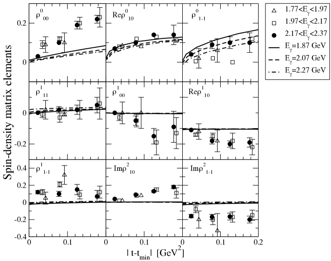
Figure 12: The density matrix elements as a function of $|t-t_{\mathrm{min}}|$ for three different photon energies, i.e. $1.87$ GeV, $2.07$ GeV, and $2.27$ GeV, to which the solid, dotted, and dot-solid curves correspond. The experimental data with three different ranges of the photon energy are taken from Ref. Chang:2010dg .

Rcently, the LEPS experiment measured the spin-density matrix elements for $\gamma p\to\phi p$ Chang:2010dg in the range of $E_{\gamma}=1.6-2.4$ GeV in which the Pomeron-exchange does not play any important role, in particular, in the present approach. Thus, we can examine the hadronic contributions to each spin-density matrix elements. Figure 12 illustrates the various spin-density matrix elements, compared with the LEPS data. Since the experimental data are given in the finite range of $E_{\gamma}$, we just take the three center values corresponding to the ranges, i.e. $E_{\gamma}=1.87,\,2.07,\,2.27$ GeV. The hadronic diagrams considered in the present work describe quantitatively $\mathrm{Re}\rho_{10}^{0}$, $\rho_{1-1}^{0}$ and $\rho_{11}^{1}$. However, the deviations are found in other spin-density matrix elements as $t-|t|_{\mathrm{min}}$ increases.

IV Summary and outlook

In the present work, we aimed at investigating the coupled-channel effects arising from the hadronic intermediate box diagrams to $\phi$ photoproduction near the threshold region in addition to the Pomeron-, $\pi$-, and $\eta$-exchanges. In particular, the bump-like structure near $E_{\gamma}\approx 2.3$ GeV, which was reported by the LEPS experiment Mibe:2005er , sheds light on the production mechanism of the $\phi$ meson in the vicinity of the threshold, since the Pomeron-exchange was shown to be not enough to explain this peculiar structure of $\phi$ photoproduction. Thus, we studied in detail the effects of the seven different box diagrams such as $\rho N$, $\omega N$, $\sigma N$, $\pi N$, $K\Lambda(1116)$, $K^{*}\Lambda(1116)$, and $K\Lambda(1520)$. In order to take into account the rescattering terms, we employed the Landau-Cutkosky rule in dealing with these box diagrams.

Since it turned out that the $K\Lambda^{*}(1520)$ box diagram played a dominant role among hadronic contributions in the lower-energy region, we scrutinized its contribution to $\phi$ photoproduction. We introduced the form factors depending on both the $s$ and $t$ Mandelstam variables in such a way that the total cross section of the $\gamma p\to K\Lambda^{*}(1520)$ reaction was well reproduced. All other box diagrams were constructed by utilizing the previous theoretical works and by reproducing the corresponding experimental data when they were available. We examined each contribution carefully by computing the differential cross section of $\phi$ photoproduction. While the $K\Lambda^{*}$ box diagram was found to be the most dominant near the 2 GeV, all other box diagrams turned out to be very small. The results were in good agreement with the LEPS data including the bump-like structure. We also computed the differential cross section as a function of $t+|t|_{\mathrm{min}}$ and found it to be in good agreement with the experimental data.

We investigated the contributions of hadronic box diagrams to the decay angular distributions. While the one-dimensional angular distributions $W(\cos\theta)$ and $W(\phi-\Phi)$ were in good agreement with the experimental data, other three angular distributions seemed to deviate from the LEPS experimental data. We also examined the various spin-density matrix elements, which were measured recently by the LEPS collaboration. We found that the hadronic box diagrams describe the experimental data for $\mathrm{Re}\rho_{10}^{0}$, $\rho_{1-1}^{0}$ and $\rho_{11}^{1}$ were well reproduced. While the present results explain near $t-|t|_{\mathrm{min}}\approx 0$ relatively well for other spin-density matrix elements, they deviated from the expeimental data as $t-|t|_{\mathrm{min}}\approx 0$ increased.

As shown in the present work, the intermediate box diagrams, in particular, the $K\Lambda^{*}(1520)$ one, play crucial roles in explaining the cross sections of the $\gamma p\to\phi p$ reaction in the vicinity of the threshold. Other box diagrams also provided certain effects on the part of the spin-density matrix elements. We have considered in this work only the imaginary part of the transition amplitudes of the box diagrams based on the Landau-Cutkosky rule. However, the results of the spin-density matrix elements already indicate that we should carry out a theoretical analysis of $\phi$ photoproduction more systematically and quantitatively. Thus, we need to investigate a full coupled-channel formalism and to solve rescattering equations with the real parts of the box diagrams fully taken into account. Another interesting and important problem is to extend our approach to the neutron target, since some of considered amplitudes are isospin-dependent. The corresponding works are under way.

Appendix A the spin-density matrix elements 

The spin-density matrix elements are expressed in terms of the helicity amplitudes Schilling:1969um ; Titov:1999eu

$$\rho_{\lambda\lambda^{\prime}}^{0} = \frac{1}{N}\sum_{\lambda_{\gamma},\lambda_{i},\lambda_{f}}T_{\lambda_{f},\lambda;\lambda_{i},\lambda_{\gamma}}T_{\lambda_{f},\lambda^{\prime};\lambda_{i},\lambda_{\gamma}}^{*},$$ (69)

$$\rho_{\lambda\lambda^{\prime}}^{1} = \frac{1}{N}\sum_{\lambda_{\gamma},\lambda_{i},\lambda_{f}}T_{\lambda_{f},\lambda;\lambda_{i},-\lambda_{\gamma}}T_{\lambda_{f},\lambda^{\prime};\lambda_{i},\lambda_{\gamma}}^{*},$$ (70)

$$\rho_{\lambda\lambda^{\prime}}^{2} = \frac{i}{N}\sum_{\lambda_{\gamma},\lambda_{i},\lambda_{f}}\lambda_{\gamma}T_{\lambda_{f},\lambda;\lambda_{i},-\lambda_{\gamma}}T_{\lambda_{f},\lambda^{\prime};\lambda_{i},\lambda_{\gamma}}^{*},$$ (71)

$$\rho_{\lambda\lambda^{\prime}}^{3} = \frac{1}{N}\sum_{\lambda_{\gamma},\lambda_{i},\lambda_{f}}\lambda_{\gamma}T_{\lambda_{f},\lambda;\lambda_{i},\lambda_{\gamma}}T_{\lambda_{f},\lambda^{\prime};\lambda_{i},\lambda_{\gamma}}^{*},$$ (72)

where $\lambda_{\gamma}$, $\lambda_{i}$, and $\lambda_{f}$ represent the helicities for the photon and the initial and final nucleons, respectively, whereas $\lambda$ and $\lambda^{\prime}$ denote those for the $\phi$ meson. The normalization factor $N$ is defined as

$$N=\sum|T_{\lambda_{f},\lambda;\lambda_{i},\lambda_{\gamma}}|^{2}.$$ (73)

References

(1)
Z. Ahmed et al. [HAPPEX Collaboration],
Phys. Rev. Lett. 108, 102001 (2012) [arXiv:1107.0913
[nucl-ex]] and references therein.
(2) S. Donnachie, G. Dosch, P. Landshoff, and
O. Nachtmann, Pomeron Physics and QCD (Cambridge University
Press, Cambridge, UK, 2002), and references therein.
(3) F.E. Close and A. Donnachie, in
Electromagnetic Interactions and Hadronic Structure edited by
F. Close, S. Donnachie, and G. Shaw, (Cambridge University Press,
Cambridge, UK, 2007).
(4)
T. Mibe et al. [LEPS Collaboration],
Phys. Rev. Lett. 95, 182001 (2005) [nucl-ex/0506015].
(5)
W. C. Chang et al. [LEPS Collaboration],
Phys. Rev. C 82, 015205 (2010) [arXiv:1006.4197 [nucl-ex]].
(6)
A. I. Titov, T. -S. H. Lee, H. Toki and O. Streltsova,
Phys. Rev. C 60, 035205 (1999).
(7) J. Beringer et al., (Particle Data Group),
Phys. Rev. D 86, 010001 (2012).
(8) S. Ozaki, A. Hosaka, H. Nagahiro and O. Scholten,
Phys. Rev. C 80, 035201 (2009)
[Erratum-ibid. C 81, 059901 (2010)] [arXiv:0905.3028[hep-ph]].
(9)
S. -I. Nam, A. Hosaka and H. -Ch. Kim,
Phys. Rev. D 71, 114012 (2005)
[hep-ph/0503149].
(10)
A. Kiswandhi and S. N. Yang,
Phys. Rev. C 86, 015203 (2012)
[Erratum-ibid. C 86, 019904 (2012)]
[arXiv:1112.6105 [nucl-th]].
(11)
A. Kiswandhi, J. -J. Xie and S. N. Yang,
Phys. Lett. B 691, 214 (2010)
[arXiv:1005.2105 [hep-ph]].
(12)
L. D. Landau,
Nucl. Phys. 13, 181 (1959).
(13)
R. E. Cutkosky,
J. Math. Phys. 1, 429 (1960).
(14)
A. Donnachie and P. V. Landshoff, Phys. Lett.
B185, 403 (1987).
(15)
A. I. Titov and T. S. H. Lee,
Phys. Rev. C 67, 065205 (2003) [nucl-th/0305002].
(16)
A. I. Titov and B. Kampfer,
Phys. Rev. C 76, 035202 (2007) [arXiv:0705.2010[nucl-th]].
(17)
R. Machleidt,
Adv. Nucl. Phys. 19, 189 (1989).
(18)
T. .A. Rijken,
Phys. Rev. C 73, 044007 (2006) [nucl-th/0603041].
(19) A. I. Titov and T. S. H. Lee, Phys. Rev. C 66, 015204 (2002)
(20)
U. -G. Meissner, V. Mull, J. Speth and J. W. van Orden,
Phys. Lett. B 408, 381 (1997) [hep-ph/9701296].
(21)
P. Mergell, U. G. Meissner and D. Drechsel,
Nucl. Phys. A 596, 367 (1996) [hep-ph/9506375].
(22)R. A. Adelseck, C. Bennhold, and L. E. Wright,
Phys. Rev. C 32, 1681 (1985).
(23)
B. Friman and M. Soyeur,
Nucl. Phys. A 600, 477 (1996)
[nucl-th/9601028].
(24)
H. Kaneko, A. Hosaka and O. Scholten,
Eur. Phys. J. A 48, 56 (2012)
[arXiv:1112.4776 [hep-ph]].
(25)
A. Kiswandhi and S. N. Yang,
AIP Conf. Proc. 1432, 323 (2012)
[arXiv:1108.1657 [nucl-th]].
(26)
K. H. Glander, J. Barth, W. Braun, J. Hannappel, N. Jopen, F. Klein,
E. Klempt and R. Lawall et al.,
Eur. Phys. J. A 19, 251 (2004) [nucl-ex/0308025].
(27)
R. Bradford et al. [CLAS Collaboration],
Phys. Rev. C 73, 035202 (2006)
(28)
M. Sumihama et al. [LEPS Collaboration],
Phys. Rev. C 73, 035214 (2006) [hep-ex/0512053].
(29)
K. Hicks et al. [LEPS Collaboration],
Phys. Rev. C 76, 042201 (2007).
(30)
P. Achenbach, C. Ayerbe Gayoso, J. C. Bernauer, S. Bianchin,
R. Bohm, O. Borodina, D. Bosnar and M. Bosz et al.,
Eur. Phys. J. A 48, 14 (2012) [arXiv:1104.4245 [nucl-ex]].
(31)
K. Hicks, D. Keller and W. Tang,
AIP Conf. Proc. 1374, 177 (2011) [arXiv:1012.3129 [nucl-ex]].
(32)
S. Janssen, J. Ryckebusch, W. Van Nespen, D. Debruyne and T. Van
Cauteren,
Eur. Phys. J. A 11, 105 (2001) [nucl-th/0105008].
(33)
Y. Oh and H. Kim,
Phys. Rev. C 73, 065202 (2006) [hep-ph/0602112].
(34)
Y. Oh and H. Kim,
Phys. Rev. C 74, 015208 (2006) [hep-ph/0605105].
(35)
B. G. Yu, T. K. Choi and W. Kim,
Phys. Lett. B 701, 332 (2011) [arXiv:1104.3672 [nucl-th]].
(36)
S. -H. Kim, S. -i. Nam, Y. Oh and H. -Ch. Kim,
Phys. Rev. D 84, 114023 (2011) [arXiv:1110.6515 [hep-ph]].
(37) K. Nakayama, Y. Oh and H. Haberzettl
Phys. Rev. C 74, 035205 (2006).
(38)
A. I. Titov, H. Ejiri, H. Haberzettl and K. Nakayama,
Phys. Rev. C 71, 035203 (2005)
[nucl-th/0410098].
(39) A. I. Titov, B. Kämpfer, B.L. Reznik
Phys. Rev. C 65, 065202 (2002).
(40) T. Sato and T.-S. H. Lee Phys. Rev. C 54,
2660 (1996).
(41)
C. Wu, J. Barth, W. Braun, J. Ernst, K. H. Glander, J. Hannappel,
N. Jopen and H. Kalinowsky et al.,
Eur. Phys. J. A 23, 317 (2005).