The effective slip-length tensor for a flow over “weakly” slipping stripes

Abstract

We discuss the flow past a flat heterogeneous solid surface decorated by slipping stripes. The spatially varying slip length, $b(y)$, is assumed to be small compared to the scale of the heterogeneities, $L$, but finite. For such “weakly” slipping surfaces, earlier analyses have predicted that the effective slip length is simply given by the surface-averaged slip length, which implies that the effective slip-length tensor becomes isotropic. Here we show that a different scenario is expected if the local slip length has step-like jumps at the edges of slipping heterogeneities. In this case, the next-to-leading term in an expansion of the effective slip-length tensor in powers of $\mbox{max}\,(b(y)/L)$ becomes comparable to the leading-order term, but anisotropic, even at very small $b(y)/L$. This leads to an anisotropy of the effective slip, and to its significant reduction compared to the surface-averaged value. The asymptotic formulae are tested by numerical solutions and are in agreement with results of dissipative particle dynamics simulations.

I Introduction

With emerging technologies in microfluidics Stone et al. (2004); Squires and Quake (2005), there has been renewed interest in quantifying the effects of surface chemical heterogeneities with local scalar slip Vinogradova (1999); Bocquet and Barrat (2007) on fluid motion. Well-known examples of such heterogeneous systems include composite superhydrophobic (Cassie) surfaces, where a gas layer is stabilized by a rough wall texture Quere (2008). These surfaces are known to be self-cleaning and show low adhesive forces. In addition, they also exhibit drag reduction for fluid flow Bocquet and Barrat (2007); McHale et al. (2010); Vinogradova and Belyaev (2011); Vinogradova and Dubov (2012). This is due to a local slip length at the gas areas, $b\simeq e(\mu/\mu_{g}-1)\simeq 50e$, where $\mu_{g}$ and $\mu$ are dynamic viscosities of a gas and a liquid, and $e$ is the thickness of the gas layer Vinogradova (1995). As a result, and in contrast to a smooth hydrophobic surfaces, where $b$ cannot exceed a few tens of nm Vinogradova and Yakubov (2003); Vinogradova et al. (2009); Cottin-Bizonne et al. (2005); Joly et al. (2006), slip lengths up to tens or even hundreds of $\mu$m may be obtained for superhydrophobic textures Choi et al. (2006); Joseph et al. (2006). Therefore, these surfaces have the potential to influence microfluidics (or to extend microfluidic systems to nanofluidics), by generating very fast and well-controlled flows in small devices Vinogradova and Belyaev (2011); Rothstein (2010); Vinogradova and Dubov (2012).

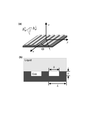
Figure 1: Sketch of the striped surface: $\Theta=\pi/2$ corresponds to transverse stripes, $\Theta=0$ to longitudinal stripes (a), and of the liquid interface in the Cassie state (b).

In case of superhydrophobic materials it is convenient to construct so-called effective slip boundary conditions, where the complex flow pattern at a heterogeneous surface is replaced by an effective flow averaged over the length scale of the experimental configuration Vinogradova and Belyaev (2011); Kamrin et al. (2010). In other words, rather than trying to solve equations of motion on the scale of the individual corrugation or pattern, one considers the “macroscale” fluid motion (on the scale larger than the pattern characteristic length) by using macroscopically equivalent boundary conditions for an imaginary smooth surface. Such an effective condition mimics the actual one along the true heterogeneous surface. It fully characterizes the flow at the real surface and can be used to solve complex hydrodynamic problems with much reduced computational effort. The effective slip approach has been supported by statistical diffusion arguments Bazant and Vinogradova (2008), and justified for the case of Stokes flow over a broad class of surfaces Kamrin et al. (2010). Several numerical approaches have recently confirmed the concept of effective slip either at the molecular scale, using molecular dynamics Priezjev (2011); Tretyakov and Müller (2013), or at larger mesoscopic scales using finite element methods Priezjev et al. (2005); Cottin-Bizonne et al. (2004), Lattice-Boltzmann Schmieschek et al. (2012); Asmolov et al. (2013) or Dissipative Particle Dynamics Zhou et al. (2012) simulations.

For an anisotropic texture, the effective boundary condition generally depends on the direction of the flow and is a tensor, $\mathbf{b}_{\mathrm{eff}}\equiv\{b_{\mathrm{eff}}^{ij}\}$, represented by a symmetric, positive definite $2\times 2$ matrix, which can be diagonalized by a rotation with angle $\Theta$ (Figure 1). For all anisotropic surfaces its eigenvalues $b_{\mathrm{eff}}^{\parallel}$ and $b_{\mathrm{eff}}^{\perp}$ correspond to the fastest (greatest forward slip) and slowest (least forward slip) orthogonal directions Bazant and Vinogradova (2008). In the general case of arbitrary direction $\Theta$, the flow past such surfaces with anisotropic effective slip becomes misaligned with the driving force. Therefore, anisotropic textures can potentially be used to generate transverse hydrodynamic flow Ajdari (2002); Bazant and Vinogradova (2008); Stroock et al. (2002a), which is of obvious fundamental and practical interest. For example, transverse hydrodynamic couplings in flow through a textured channel can be used to separate/concentrate suspended particles Gao and Gilchrist (2008) or for passive chaotic mixing Stroock et al. (2002a, b). This can also be used to generate anisotropic electrokinetic flows Bahga et al. (2010); Belyaev and Vinogradova (2011); Squires (2008).

However, it has been predicted that regardless of the anisotropy of the surface texture, the effective slip-length tensor, $\mathbf{b}_{\mathrm{eff}}$, becomes isotropic ($b_{\mathrm{eff}}^{\perp}=b_{\mathrm{eff}}^{\parallel}$) for a “weakly” slipping pattern, i.e. when the local slip length, $b(x,y)$, is small compared to the characteristic scale of heterogeneities, $L$. The value of the effective slip is the surface average of the local slip length, $\mathbf{b}_{\mathrm{eff}}=\mathbf{I}\,\langle b(x,y)\rangle$. In the particular case of a no-slip plane covered by patterns with constant slip length $b$ – the situation considered in most previous publications on the subject  Priezjev et al. (2005); Ybert et al. (2007); Feuillebois et al. (2009) – one can derive Ybert et al. (2007); Belyaev and Vinogradova (2010); Kamrin et al. (2010)

$$b_{\mathrm{eff}}^{\parallel,\perp}\simeq b\phi,$$ (1)

where $\phi=\delta/L$ is the surface fraction of the slipping phase. We remark and stress that $b_{\mathrm{eff}}^{\parallel,\perp}$ can still remain extremely large compared to the nanometric scalar slip at flat hydrophobic solids. Eq. (1) implies, among other, that the flow aligns with the applied driving force for all in-plane directions. Thus, it seems impossible to generate transverse hydrodynamic Vinogradova and Belyaev (2011); Zhou et al. (2012) or transverse electro-osmotic Belyaev and Vinogradova (2011) phenomena for “weakly” slipping anisotropic textures. Another important, and somewhat remarkable, consequence of Eq. (1) is that the effective slip is predicted to depend only on the fractions of slipping areas, but not on their detailed structure.

Known derivations of Eq. (1), however, neglect localized flow perturbations around possible jumps in discrete slip lengths, from 0 to $b$, at the border of heterogeneities. Such jumps could contribute to the friction, as has been recently detected in a molecular dynamics simulation study Tretyakov and Müller (2013), and also to the anisotropy of the flow, but we are not aware of any prior work that has quantified the phenomena. In this paper we reconsider the problem of flow past “weakly” slipping one-dimensional surfaces, focusing on the situation of superhydrophobic stripes, where the perturbation of $b(y)$ is piecewise constant, i.e., it jumps in a step-like fashion at heterogeneity boundaries.

Our paper is arranged as follows: In Sec. II we define the problem and construct the expansions for the eigenvalues of the slip-length tensor of alternating “weakly” slipping stripes. Here we also analyze a singularity of the velocity gradient at the edges of stripes. The details of the computer simulation method (dissipative particle dynamics) related to “weakly” slipping surfaces are discussed in Sec. III. Finally, in Sec. IV, we present simulation and numerical results to validate the predictions of the asymptotic theory. The practical implications and limitations of our models are also reviewed here. In Appendix A we give some simple arguments showing that standard two-term expansions for effective slip lengths of one-dimensional textures could not be applied in case of a discontinuous local slip.

II Theory

II.1 Problem Set-up

We consider a creeping flow along a planar anisotropic wall, and a Cartesian coordinate system $(x,y,z)$ (Figure 1). The origin of coordinates is placed at the flat interface, a one-dimensional texture varies over a period $L$. Our analysis is based on the limit of a thick channel or a single interface, so that the velocity profile sufficiently far above the surface may be considered as a linear shear flow. Dimensionless variables are defined in terms of the reference length scale $L$, the asymptotic shear rate far above the surface, $G,$ and the fluid kinematic viscosity, $\nu.$

For a one-dimensional texture there exists a simple relation between longitudinal and transverse effective slip lengths Asmolov and Vinogradova (2012)

$$b_{\mathrm{eff}}^{\perp}[b\left(y\right)]=\frac{b_{\mathrm{eff}}^{\parallel}\left[2b\left(y\right)\right]}{2},$$ (2)

which has recently been verified for cosine variation in local slip length by using lattice Boltzmann simulations Asmolov et al. (2013). Therefore, it is sufficient to consider the longitudinal configuration. Since in this case, the velocity has only one component, we seek a solution for the velocity profile of the form

$$v=U+u,$$

where $U=z\$is the undisturbed linear shear flow. The perturbation of the flow $u\left(y,z\right)$, which is caused by the presence of the texture and decays far from the surface at small Reynolds number $Re=GL^{2}/\nu$, satisfies the dimensionless Laplace equation,

$$\Delta u=0.$$ (3)

The boundary conditions at the wall and at infinity are defined as

$$z=0: u-\varepsilon\beta\left(y\right)\partial_{z}u=\varepsilon\beta\left(y\right),\$$ (4)

$$z\rightarrow\infty: \partial_{z}u=0\mathbf{,}$$ (5)

where $\varepsilon=\mbox{max}\,(b(y))/L\$and $\beta=b\left(y\right)/\mbox{max}\,(b(y))$ is the normalized slip length.

The solution of Eqs. (3)-(5) for a “weakly” slipping anisotropic texture, $\varepsilon\ll 1$, can be constructed as an expansion in powers of $\varepsilon$ :

$$u=\sum\limits_{k=1}^{\infty}\varepsilon^{k}\varphi_{k}.$$ (6)

The boundary conditions to $\varphi_{k}$ can be readily obtained by substituting Eq. (6) into Eq. (4) and by collecting the terms of the order of $\varepsilon^{k}$ Kamrin et al. (2010):

$$\begin{array}[]{rcl}z=0:&&\varphi_{1}=\beta\left(y\right),\\ z=0,\ k>1:&&\varphi_{k}=\beta\left(y\right)\partial_{z}\varphi_{k-1}.\end{array}$$ (7)

The leading-order solution yields an area-averaged isotropic slip length Ybert et al. (2007); Belyaev and Vinogradova (2010). In practice, this means that the slip-length tensor becomes isotropic and that for all in-plane directions, the flow aligns with the applied force.

It is important to note however that Eqs.(6) and (7) are inapplicable for a discontinuous $\beta(y)$ (see Appendix A for details). From a physical point of view, the problem is associated with singularities of the velocity gradient at the boundaries of the slip region. As a specific example, let us consider a classical case of alternating “weakly” slipping ($\varepsilon=b/L\ll 1$) stripes with

$$\beta\left(y\right)=\left\{\begin{array}[]{cl}1&\text{ as }\left|y\right|\leq\phi/2\\ 0&\text{ as }\phi/2<\left|y\right|\leq 1/2\end{array}\right.,$$ (8)

so that the boundary conditions, Eq. (4), can be rewritten as

$$\begin{array}[]{rcl}z=0,\ \left|y\right|\leq\phi/2:&&u-\varepsilon\partial_{z}u=\varepsilon,\\ z=0,\ \phi/2<\left|y\right|<1/2:&&u=0.\end{array}$$ (9)

The velocity gradient grows infinitely near the edge of the slip region (see Sec. II.3 for a detailed analysis). As a result, the corresponding term in Eq. (9), $\varepsilon\partial_{z}u$, has the same order of magnitude as $u$ in the vicinity of the slipping boundary. Therefore, it cannot be neglected compared to the leading order, even though $\varepsilon$ is small.

II.2 Slip-length tensor

We now consider the case of stripes more specifically. We first compute the eigenvalues of the effective slip-length tensor. Since we assume only weak local slippage, we evaluate the effective slip length in the principal directions to second order in $\varepsilon$ and seek for a solution which is finite, i.e., has no singularity.

A general solution satisfying the Laplace equation (3) and decaying at infinity can be presented in terms of a cosine Fourier series as Asmolov and Vinogradova (2012)

$$u=\frac{a^{0}}{2}+\sum\limits_{n=1}^{\infty}a^{n}\exp\left(-2\pi nz\right)\cos\left(2\pi ny\right),$$ (10)

where $a^{n}$ are constant coefficients to be found from (9). The Navier slip boundary condition (4) can be written in terms of the Fourier coefficients $a^{n},$ accounting for (10), as

$$\frac{a^{0}}{2}+\sum_{n=1}^{\infty}\left[1+2\pi n\varepsilon\beta\left(y\right)\right]a^{n}\cos\left(2\pi ny\right)=\varepsilon\beta\left(y\right).\$$ (11)

We construct the asymptotic series for alternating stripes,

$$u=\sum\limits_{k=1}^{\infty}u_{k}=\sum\limits_{k=1}^{\infty}\left[\frac{a_{k}^{0}}{2}+\sum\limits_{n=1}^{\infty}a_{k}^{n}\exp\left(-2\pi nz\right)\cos\left(2\pi ny\right)\right],$$

imposing that $\left|u_{k+1}/u_{k}\right|\ll 1$ over the entire flow region. The boundary conditions for $u_{k}$ at the wall can be chosen as follows:

$$z=0:\quad u_{k}-\varepsilon\partial_{z}u_{k}=r_{k}\left(y\right),$$ (12)

$$r_{1}\left(y\right)=\left\{\begin{array}[]{rl}\varepsilon&\text{ as }\left|y\right|\leq\phi/2\\ 0&\text{ as }\phi/2<\left|y\right|\leq 1/2\end{array}\right.,$$ (13)

$$k>1:\quad r_{k}\left(y\right)=\left\{\begin{array}[]{cl}0&\text{ as }\left|y\right|\leq\phi/2\\ -\varepsilon\partial_{z}u_{k-1}&\text{ as }\phi/2<\left|y\right|\leq 1/2\end{array}\right..$$ (14)

The reader may check by the summation of Eqs. (12) over $k$ that they are fully equivalent to Eq. (9).

The slip velocity is the average velocity over the period:

$$u_{slip}=\sum\limits_{k=1}^{\infty}a_{k}^{0}/2.$$

The boundary condition (12) can be rewritten in view of (11) as

$$\frac{a_{k}^{0}}{2}+\sum\limits_{n=1}^{\infty}a_{k}^{n}\left(1+2\pi\varepsilon n\right)\cos\left(2\pi ny\right)=r_{k}\left(y\right).$$

The coefficients $a_{k}^{n}$ are now determined using the inverse Fourier transform:

$$a_{k}^{0} = 2\int_{-1/2}^{1/2}r_{k}\left(y\right)dy,$$ (15)

$$n>0:\quad a_{k}^{n} = \frac{2}{1+2\pi\varepsilon n}\int_{-1/2}^{1/2}r_{k}\left(y\right)\cos\left(2\pi ny\right)dy.$$

From Eqs. (13) and (15), we have to leading order in $\varepsilon$

$$a_{1}^{0} = 2\varepsilon\phi,$$

$$n>0:\quad a_{1}^{n} = \frac{2\varepsilon\sin\left(\pi n\phi\right)}{\pi n\left(1+2\pi\varepsilon n\right)}.$$

To find the second-order terms we must evaluate $r_{2}=\partial_{z}u_{1}$, which gives

$$\partial_{z}u_{1} = -\sum\limits_{n=1}^{\infty}a_{1}^{n}2\pi n\cos\left(2\pi ny\right)$$ (16)

$$= -4\varepsilon\sum\limits_{n=1}^{\infty}\frac{\sin\left(\pi n\phi\right)\cos\left(2\pi ny\right)}{1+2\pi\varepsilon n}.$$

The second-order slip velocity is then

$$a_{2}^{0}=-4\int_{\phi/2}^{1/2}\varepsilon\partial_{z}u_{1}dy=-\frac{4\varepsilon^{2}}{\pi}\sum\limits_{n=1}^{\infty}\frac{1-\cos\left(2\pi n\phi\right)}{n\left(1+2\pi\varepsilon n\right)}$$ (17)

$$=\frac{4\varepsilon^{2}}{\pi}\left\{\ln\left(2\pi\varepsilon\right)-\gamma-\frac{1}{2}\ln\left[4\sin^{2}\left(\pi\phi\right)\right]\right\}+O\left(\varepsilon^{3}\right),$$ (18)

where $\gamma=0.5772157...$ is Euler’s constant. The series in Eq. (17) are very similar to those expected for a discontinuous $b(y)$ (see Eq. (41) of Appendix A). They differ only by the factor $(1+2\pi\varepsilon n)$ in the denominator of the first sum. This factor is small at $n=1,$ but it grows linearly with $n$ at large $n$, thus ensuring convergence of the series. Note that the first logarithmic term in (18) does not depend on the fraction of the slip regions, $\phi.$ This term is associated with the flow singularities near the boundaries between no-slip and slip regions (see Subsection II.3), which are responsible for additional viscous dissipation that reduces $b_{\mathrm{eff}}.$

Finally, for the longitudinal effective slip we obtain the following expansion

$$b_{\mathrm{eff}}^{\parallel}/L=\varepsilon\phi+\frac{2\varepsilon^{2}}{\pi}\left\{\ln\left[\frac{\pi\varepsilon}{\sin\left(\pi\phi\right)}\right]-\gamma\right\}+O\left(\varepsilon^{3}\ln\varepsilon\right),$$ (19)

from which we can derive the transverse effective slip using (2),

$$b_{\mathrm{eff}}^{\perp}/L=\varepsilon\phi+\frac{4\varepsilon^{2}}{\pi}\left\{\ln\left[\frac{2\pi\varepsilon}{\sin\left(\pi\phi\right)}\right]-\gamma\right\}+O\left(\varepsilon^{3}\ln\varepsilon\right).$$ (20)

To summarize, we have here directly demonstrated that Eq. (1) must be applied with care. On the one hand, Eqs. (19) and (20) unambiguously show that  Eq. (1) does indeed give the correct first-order term of an expansion for the eigenvalues of the slip-length tensor, even in a case of alternating stripes. On the other hand, the higher order contributions may be nonanalytical in $\varepsilon$, which may create complications. In case of a local slip which exhibits step-like jumps at the edge of heterogeneities, the second-order terms of the expansions become of the order of $\varepsilon^{2}\ln\varepsilon$ (in contrast to $\varepsilon^{2},$ which would be expected for continuously varying local slip). Therefore, they can be comparable to the first-order terms and cannot be ignored even at relatively small $\varepsilon$ (see Section IV). These terms are not only responsible for anisotropy of the flow, but also (being negative) for an additional dissipation.

II.3 Edge singularity

We now describe the flow singularities near slipping heterogeneities in more detail. For the flow over a surface with rectangular grooves, the shear stress is found to be singular near sharp corners, i.e., proportional to $r^{-1/3}$ for longitudinal and to $r^{-0.455}$, for transverse configurations Wang (2003). Here $r$ is the distance from the corner. Following this approach, we now consider the flow in the vicinity of the edge of our “weakly” slipping regions, by using polar coordinates $(r,\theta)$ with the origin in $\left(y,z\right)=\left(\phi/2,0\right)$. The no-slip and slip regions then correspond to $\theta=0\$and $\theta=\pi$. The solution of the Laplace equation (3) that satisfies the no-slip boundary condition at $\theta=0$ is

$$u=cr^{\lambda}\sin\left(\lambda\theta\right).$$ (21)

The velocity at the edge is finite provided $\lambda>0.$ The components of velocity gradient are

$$\partial_{z}u = c\lambda r^{\lambda-1}\cos\left[\theta\left(1-\lambda\right)\right],$$

$$\partial_{y}u = -c\lambda r^{\lambda-1}\sin\left[\theta\left(1-\lambda\right)\right].$$ (22)

The velocity decays faster than its gradient as $r\rightarrow 0:$ $r^{\lambda}$ vs. $r^{\lambda-1}.$ Hence, in a small region $r\sim\varepsilon,$ the dimensionless shear rate $\varepsilon\partial_{z}u$ is of the same order as $u,$ and cannot be ignored in the boundary condition (9) even though $\varepsilon\ll 1.$ Moreover, at smaller distances, $r\ll\varepsilon,$ the term $\varepsilon\partial_{z}u$ dominates over $u$, and the condition in this region becomes shear-free:

$$r\ll\varepsilon,\ \theta=\pi:\quad\partial_{z}u=0.$$ (23)

The last condition enables us to find $\lambda$. To satisfy Eq. (23) one should require, in view of (22), $\lambda=1/2.$ Therefore, the velocity over the slip region is

$$r\ll\varepsilon,\ \theta=\pi:\quad u=cr^{1/2},\quad\partial_{y}u=-cr^{-1/2}/2,$$ (24)

where $c$ is a constant. The velocity gradient over the no-slip region follows from (22):

$$r\ll\varepsilon,\ \theta=0:\quad\partial_{z}u=cr^{-1/2}/2.$$ (25)

In other words, the shear stress has a singularity at the edge.

We remark that Eqs. (24) and (25) are valid in a small region, $r\ll\varepsilon,$ near a jump in the discrete local slip length, from $0$ to a finite $b.$ Therefore, our asymptotic theory is only valid provided that the fractions of the slip and no-slip regions are not too small, $\phi\gg\varepsilon,\ 1-\phi\gg\varepsilon.$ Otherwise, the two edges of heterogeneities are close to each other, so that the singular regions overlap. Note that a similar, $r^{-1/2}$, dependence of the velocity has been obtained earlier for a no-slip surface decorated with perfect-slip stripes Philip (1972); Sbragaglia and Prosperetti (2007); Asmolov and Vinogradova (2012). A striking conclusion from our analysis is that such a singularity appears even at a very small slip at the gas area.

For the transverse flow one can use the relation between the velocity fields for the two orientations Asmolov and Vinogradova (2012):

$$v=\frac{1}{2}\left(u_{d}+z\frac{\partial u_{d}}{\partial z}\right),\quad w=-\frac{z}{2}\frac{\partial u_{d}}{\partial y},$$ (26)

$$p=-\frac{\partial u_{d}}{\partial y},$$ (27)

where $u_{d}\left(y,z\right)=u\left[y,z,2\varepsilon\beta\left(y\right)\right]$ is the velocity field for the longitudinal pattern with double local slip length (cf. Eq. (2)). Hence we conclude that at the wall

$$z=0:\quad v=\frac{1}{2}u_{d},\quad\frac{\partial v}{\partial z}=\frac{\partial u_{d}}{\partial z}.$$ (28)

From Eqs. (24) - (27), it also follows that $\frac{\partial v}{\partial z},$ $\frac{\partial w}{\partial z}$ and $p$ all have the same singularity $r^{-1/2}$ at the edge of “weakly” slipping region.

III Simulation method

We apply Dissipative Particle Dynamics (DPD) method Hoogerbrugge and Koelman (1992); Español and Warren (1995); Groot and Warren (1997) to simulate the flow near striped superhydrophobic surfaces. The DPD method is an established coarse-grained, momentum-conserving method for mesoscale fluid simulations, which naturally includes thermal fluctuations. More specifically, we use a DPD version without conservative interactions Soddemann et al. (2003). The hydrodynamic boundary conditions are implemented using the tunable-slip method Smiatek et al. (2008), which model the fluid/surface interaction using an effective friction force, combined with an appropriate thermostat.

The error of the simulation data is obtained from averaging over six independent runs. The absolute error in the effective slip length is typically around $0.2\,\sigma$, where $\sigma$ is the length unit in the simulation (see Appendix B for details). For “weakly” slipping surfaces, the ratio between the effective slip length and the stripe spacing is of the order of $b_{\rm eff}/L\sim 0.1$. One can then improve the accuracy by choosing a large $L$. On the other hand, the size of the simulation box is proportional to $L^{2}$, and the time for the system to reach a steady state also increases for a large system. Therefore, the choice of the stripe spacing is a compromise between the computational accuracy and time. In this study, we have used a stripe spacing of $L=100\sigma$ and a simulation box of size $20\sigma\times 100\sigma\times 102\sigma$. With a density of $3.0\,\sigma^{-3}$, a typical system consists of $6\times 10^{5}$ particles. The simulations are carried out using the open source simulation package ESPResSo Limbach et al. (2006).

Based on the values of the velocities close to the surface, we can estimate the characteristic Reynolds number of our system to be of $O(10)$, which is larger than in real microfluidic devices. Thus, inertia effects may become important in simulations, and the Stokes equation is not strictly valid. This leads to a slight reduction of our simulation results for the effective slip length transverse stripes as we discuss below. To reach more realistic Reynolds numbers, we would need to reduce the shear rate by orders of magnitude. This would reduce the average flow velocity significantly, and the necessary simulation time to gather data with sufficiently good statistics will then increase prohibitively.

IV Results and Discussion

In this section, we compare predictions of our asymptotic theory with results of DPD simulations and direct numerical solutions of Eqs. (3)-(5). To find $a^{n}$ numerically we truncate the sum in (11) at some cut-off number $N$ (usually $N=501$) and evaluate it in the points $y_{l}=l/2\left(N-1\right),$ where $l$ are numbers varying from $0$ to $N-1$. Then Eq. (11) is reduced to a linear system $A_{n}^{l}a^{n}=\varepsilon\beta^{l},$ where $A_{n}^{l}=\left[1+2\pi n\varepsilon\beta\left(y_{l}\right)\right]\cos\left(2\pi ny_{l}\right)$ and $\beta^{l}=\beta\left(y_{l}\right).$ The system is solved using the IMSL routine LSARG.

Figures 2(a) and (b) show the exact numerical results and DPD simulation data for the longitudinal component of the slip-length tensor as a function of the dimensionless slip length $b/L$ and the slipping area $\phi$. The simulation data are in excellent agreement with the numerical results, confirming the validity of our DPD scheme. Similar calculations were made for the transverse component of the slip-length tensor. All curves were found to be very similar to those presented in Figures 2, therefore, we do not show them here. The values for the transverse component are smaller than those for the longitudinal component, indicating that the flow is anisotropic. The simulation data in the transverse case tend to be slightly smaller than the prediction from the numerical solution. This has been observed previously Zhou et al. (2012) and can be related to the relatively large Reynolds numbers in our system (see Sec. III). Inertia effects influence the flow past transverse stripes, as will be discussed below in the context of Figure 4. For flow past longitudinal stripes, $\mathbf{u}=\left(u\left(y,z\right),0,0\right)$, the inertia effects are negligible, since convective terms in the Navier-Stokes equations, $\left(\mathbf{u\cdot\nabla}\right)\mathbf{u}=\mathbf{0}$. Thus the DPD data shown in Fig. 2 are not affected by Reynolds number.

Figure 2: The longitudinal effective slip length as functions of (a) the local slip for the texture with $\phi=0.3$, and (b) the fraction of the slipping phase at $b/L=0.034$. Symbols are simulation data. Dash-dotted curves show exact numerical results, solid lines correspond to the two-term logarithmic expansions (Eq. (19)), dash lines to the linear theory (Eq. (1)), dotted lines to Eq. (29).

The surface-averaged slip, predicted by Eq. (1), is also shown in Figure 2 and is well above the exact values of the longitudinal effective slip. Also included in Figure 2 are the predictions of our theoretical result, Eq. (19). One can see that Eq. (19) indeed gives the correct asymptotic behavior in the limit of very small $b/L$. It slightly overestimates the value of the longitudinal effective slip at larger $b/L$. We remark and stress that nevertheless, our second-order calculation is much more accurate than Eq. (1).

Recently, Belyaev and Vinogradova (2010) suggested approximate expressions for effective slip lengths of a surface decorated by partial slip stripes:

$$b_{\mathrm{eff}}^{\parallel}\simeq\frac{L}{\pi}\frac{\ln\left[\sec\left(\displaystyle\frac{\pi\phi}{2}\right)\right]}{1+\displaystyle\frac{L}{\pi b}\ln\left[\sec\displaystyle\left(\frac{\pi\phi}{2}\right)+\tan\displaystyle\left(\frac{\pi\phi}{2}\right)\right]},$$ (29)

$$b_{\mathrm{eff}}^{\perp}\simeq\frac{L}{2\pi}\frac{\ln\left[\sec\left(\displaystyle\frac{\pi\phi}{2}\right)\right]}{1+\displaystyle\frac{L}{2\pi b}\ln\left[\sec\displaystyle\left(\frac{\pi\phi}{2}\right)+\tan\displaystyle\left(\frac{\pi\phi}{2}\right)\right]}.$$ (30)

These formulae have been verified Belyaev and Vinogradova (2010) using the method developed by Cottin-Bizonne et al. (2004). The agreement between the theoretical and numerical data was found to be very good for all $\phi$ and $b/L$, but at $b/L=O(1)$, small discrepancies were observed, suggesting that Eqs. (29) and (30) slightly underestimate the effective slip length. To examine this more closely, we also include the prediction of Eq. (29) in Figure 2. We find indeed a small discrepancy between the exact numerical data and the predictions of Eq. (29), which gives smaller values for the slip length. The same trends were observed in a wide range of $\phi$, and the discrepancy slightly increases with the fraction of slipping phase. Still, the analytical expressions for the effective slip by Belyaev and Vinogradova (2010) appear to be surprisingly accurate, given their simplicity. We stress, however, that they do not reproduce the asymptotic result, Eq. (1), in the limit of very small $b/L$. They do correctly predict a linear dependence on $b$ in the limit of “weakly” slipping stripes

$$b_{\mathrm{eff}}^{\parallel}=b_{\mathrm{eff}}^{\perp}\simeq f(\phi)\,b,$$ (31)

but the prefactor, $f(\phi)$, differs from $\phi$:

$$f(\phi)\simeq\frac{\ln\left[\sec\left(\frac{\pi\phi}{2}\right)\right]}{\ln\left[\sec\left(\frac{\pi\phi}{2}\right)+\tan\left(\frac{\pi\phi}{2}\right)\right]}<\phi$$ (32)

This prefactor corresponds to the slope of the curve $b_{\mathrm{eff}}^{\parallel}\left(b\right)$ at $b/L=0$. In Figure 2, the slope of the dotted line corresponding to Eq. (29) is smaller than the exact one. Nevertheless, the values of $b_{\mathrm{eff}}^{\parallel}$ and $b_{\mathrm{eff}}^{\perp}$ given by (29) and (30) correlate well with the numerical data for all $\phi$ and small but finite $b/L.$

Figure 3: The difference between longitudinal and transverse effective slip lengths as functions of (a) the local slip for textures with $\phi=0.3$, and (b) $\phi$ for textures with $b/L=0.034$. Solid curves correspond to calculations made with the two-term logarithmic expansions (Eq. (33)). Dotted curves are obtained using Eqs. (29) and (30). Other notations are the same as in Figure 2.

To summarize, “weakly” slipping stripes generate anisotropic effective slippage compared to simple, smooth channels, an ideal situation for various potential applications. To illustrate this, we now show that our results may be used to easily quantify transverse phenomena (important for a passive microfluidic mixing) and a reduction of the hydrodynamic drag force.

We begin by discussing a transverse flow, or the flow anisotropy, which in a thick channel has been predicted to be controlled by the difference between the eigenvalues of the effective slip tensor, $b_{\mathrm{eff}}^{\parallel}-b_{\mathrm{eff}}^{\perp}$, which in turn depends on $\phi$ and $b$ Vinogradova and Belyaev (2011). According to Eq. (1), this difference should vanish for “weakly” slipping surfaces. The effect of anisotropy is highlighted in Figure 3(a) and (b), which shows the difference between the longitudinal and transverse effective slip lengths computed for fixed $\phi=0.3$ and $b/L=0.034$, respectively. The exact numerical values are positive, except in the case of extremely small local slip, clearly showing that the flow is anisotropic. This is confirmed by the simulation results. The error bars are relatively large. For “weakly” slipping surfaces, the difference $b_{\mathrm{eff}}^{\parallel}-b_{\mathrm{eff}}^{\perp}$ is small compared to the slip lengths themselves, (of the order of $\varepsilon^{2}\ln\varepsilon$), and this is the reason for the large error of the simulation data. The simulation data agree with the numerical results within the error. Nevertheless, the data suggest that they lie systematically above the numerical results especially for larger slipping phase fraction $\phi$. This is a consequence of the relatively large Reynolds number. As discussed above, inertia effects primarily affect the flow and effective slip length in the transverse configuration. Test runs with larger shear rates were performed, and the deviations increased, indicating that they presumably vanish in the Stokes limit. Note that there has been recent (finite element method) work that observed the decrease of superhydrophobic slip at large Reynolds numbers Cao et al. (2012), which is consistent with our results.

Now, we remark that further insight can be obtained from the above asymptotic results, Eqs. (19) and (20), to predict the dependence $b_{\mathrm{eff}}^{\parallel}-b_{\mathrm{eff}}^{\perp}$ on parameters of the texture:

$$\frac{b_{\mathrm{eff}}^{\parallel}-b_{\mathrm{eff}}^{\perp}}{L}\simeq-\frac{2b^{2}}{\pi L^{2}}\left\{\ln\left[\frac{4\pi b}{L\sin\left(\pi\phi\right)}\right]-\gamma\right\}$$ (33)

These values are also included in Figure 3. Eq. (33), which can easily be handled, demonstrates the power of the asymptotic approach in deriving relevant expression for a difference in eigenvalues of the slip-length tensor. In the limit of small $b/L$, the asymptotic expansion predicts correctly the positive difference and enhanced anisotropy as the slip length increases. At larger $b/L$, deviations from the numerical results become larger due to the increasing contribution from higher order terms. At $b/L=0.034$, the two-term prediction for the slip length difference is only in moderately good agreement with the numerical data. For very low or very high coverage ($\phi\to 0$ or $\phi\to 1$), the agreement is not good at all, the theory even predicts the wrong sign (not shown in Figure 3(b)). This is consistent with our discussion in Section II.3, where we have argued that the approximation must break down when the singular regions associated with adjacent edges overlap. Also included in Figure 3 is the result from the approximate expressions Eqs. (29) and (30), which again shows surprisingly good agreement with the numerical data over the whole range of $\phi$.

Our theory also allows one to quantify the drag force acting on a hydrophilic sphere approaching a “weakly” slipping stripes. It has been shown that such a geometry of configuration is equivalent to a sphere approaching the imaginary smooth homogeneous isotropic surface shifted to a distance $s$ equal to the average of the eigenvalues of the effective slip-length tensor Asmolov et al. (2011)

$$s\simeq\frac{b_{\mathrm{eff}}^{\parallel}+b_{\mathrm{eff}}^{\perp}}{2}$$ (34)

The correction to a drag force due to superhydrophobic slip is then $f^{\ast}\simeq 1-s/h$ Asmolov et al. (2011); Lecoq et al. (2004). By using Eqs. (19) and (20) we could now easily relate $s$ to texture parameters by a simple analytical formula

$$\frac{s}{b}\simeq\phi+\frac{b}{\pi L}\left[\ln\left(\frac{4\pi^{3}b^{3}}{L^{3}\sin^{3}(\pi\phi)}\right)-3\gamma\right]$$ (35)

Eq. (35) can be also used in case of a plane decorated with shallow hydrophilic grooves, i.e. when the height of the texture, $e$, which should be used instead of $b$ then, is much smaller than $L$. This expression explains qualitatively recent experimental observations, where $s/e$ was found to be much smaller than $\phi$ Mongruel et al. (2013). Unfortunately detailed quantitative comparison between the experimental results  Mongruel et al. (2013) and our asymptotic predictions are impossible since the height of asperities in these experiments was not small enough, $0.168\leq e/L\leq 0.45$.

Finally, we consider the velocity at the wall near the edge of a heterogeneity. Figure 4(a) presents the longitudinal velocity at the wall for various $b/L$. In the simulations, the slip velocity has been obtained from an extrapolation procedure. Due to the small magnitude of the slip velocity in comparison to the thermal fluctuation (order of 1 for $k_{B}T=1\epsilon$), the data scatter very much. Much longer averaging times would be necessary to improve the statistics. The agreement of the exact numerical results and DPD simulation data is again very good. The velocity distribution is not smooth at the edge, instead it rises according to a power law on the slipping area with exponent close to $\lambda=0.5$ as predicted in Section II.3. In Figure 4(b), we verify the relation between the transverse and longitudinal velocities. Eq. (28) suggests that the local slip velocity above transverse stripes of slip length $b$ should be identical to half of that above longitudinal stripes of slip length $2b$. This is confirmed by the numerical results. The simulation data, however, show deviations near the edge. This illustrates the origin of the finite Reynolds number effects discussed above. In simulations, the fluid is modelled as DPD particles with finite mass, and abrupt changes of the transverse velocity are suppressed because of inertia. Therefore the transverse velocity is smoothed out near the edge, showing a smaller value compared to the numerical data.

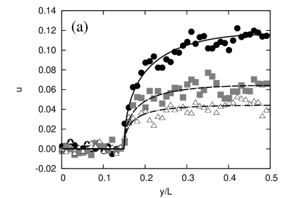
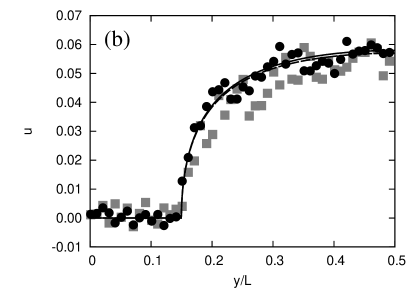
Figure 4: (a) The longitudinal velocity along the wall for a texture with $\phi=0.7$ and different slip lengths: $b/L=0.145$ (circles and solid line), $b/L=0.071$ (squares and dashed line), and $b/L=0.047$ (triangles and dash-dotted line). Symbols are simulation data and lines are numerical results. (b) Comparison of the transverse velocity ($v[y,z=0,\beta(y)]$) and longitudinal velocity for nearly double local slip length ($\frac{1}{2}u_{d}[y,z=0,2\beta(y)]$, see Eq. (28)). The simulation and numerical results for longitudinal stripes of $b/L=0.147$ are shown in circles and solid line, respectively. Squares and dashed line correspond to transverse stripes of $b/L=0.071$.

V Concluding Remarks

In conclusion, we have investigated shear flow past “weakly” slipping super-hydrophobic stripes, focusing in particular on edge effects associated with steplike discontinuities in the local slip length. The essential conclusion from our analysis is that such step effects reduce the effective slip below the surface-averaged value and induce anisotropy. In practice, this means that the flow does not align with the applied shear stress. Thus, it should be possible to generate transverse hydrodynamic phenomena (like in  Stone et al. (2004); Vinogradova and Belyaev (2011)) even with such “weakly” slipping anisotropic textures. This may also have relevance for transverse electrokinetic phenomena Bahga et al. (2010); Vinogradova and Belyaev (2011); Squires (2008); Belyaev and Vinogradova (2011). As a side remark, our analytical result opens the possibility of solving analytically many fundamental problems involving “weakly” slipping heterogeneous surfaces, including hydrodynamic interactions.

Finally, we note that even though our discussion has been limited to “weakly” slipping heterogeneities, our model is much more general. Every result in this work could be used for describing “weakly” rough or porous surfaces since at large distances from the wall, the boundary condition at the rough interface or fluid-porous interface may be approximated by a slip model Beavers and Joseph (1967); Taylor (1971); Richardson (1971); Kunert and Harting (2007); Kunert et al. (2010); Lecoq et al. (2004). In particular, our results allows one to interpret recent experiments with hydrophilic grooves, where even at small $e/L$ the model of “average height” significantly overestimated measured data Mongruel et al. (2013).

Appendix A Divergence of the expansion (6), (7) for a discontinuous local slip length

We consider periodic textures with $\beta\left(y\right)$ being an even function, so that the slip length can be expanded as a cosine Fourier series:

$$\beta=\frac{\widetilde{\beta}^{0}}{2}+\sum\limits_{n=1}^{\infty}\widetilde{\beta}^{n}\cos\left(2\pi ny\right),$$ (36)

$$\widetilde{\beta}^{n}=2\int_{-1/2}^{1/2}\beta\left(y\right)\cos\left(2\pi ny\right)dy.$$ (37)

The expansions of the effective slip lengths up to second order in $\varepsilon$ are then given by Kamrin et al. (2010)

$$b_{\mathrm{eff}}^{||}/L = \varepsilon\frac{\widetilde{\beta}^{0}}{2}-\varepsilon^{2}\pi\sum\limits_{n=1}^{\infty}n\left|\widetilde{\beta}^{n}\right|^{2},$$ (38)

$$b_{\mathrm{eff}}^{\bot}/L = \varepsilon\frac{\widetilde{\beta}^{0}}{2}-\varepsilon^{2}2\pi\sum\limits_{n=1}^{\infty}n\left|\widetilde{\beta}^{n}\right|^{2}.$$ (39)

The first-order terms are the isotropic part of the effective slip, Eq. (1), since $\widetilde{\beta}^{0}=2\,\langle\beta(y)\rangle$. The second-order terms, which can be neglected for a “weakly” slipping patterns, are expected to introduce the influence of the surface structure, and are responsible for the anisotropy of the flow.

The expansion (6), (7) implicitly assumes that the infinite sums over $n$ in the higher-order expansion coefficients converge, which implies that the Fourier series, Eq. (36), can be differentiated infinitely often with respect to $y$. In cases of discontinuous slip, where $\beta(y)$ exhibits jumps, this is no longer correct and the argument breaks down.

The Fourier coefficients for the striped texture follow from Eq. (37)

$$\widetilde{\beta}^{0}=2\phi,$$ (40)

$$n>0:\quad\widetilde{\beta}^{n}=\frac{2\sin\left(\pi n\phi\right)}{\pi n}.$$

This implies that series in Eqs. (38) and (39),

$$\sum\limits_{n=1}^{\infty}n\left|\widetilde{\beta}^{n}\right|^{2}=\frac{2}{\pi^{2}}\sum\limits_{n=1}^{\infty}\frac{1-\cos\left(2\pi n\phi\right)}{n},$$ (41)

diverge, since their terms decay as $n^{-1}$ at $n\rightarrow\infty$ (large $n$ correspond to small length scales). The slow decay of $\left|\widetilde{\beta}^{n}\right|^{2}$ with $n$ and the divergence of the series indicate that the expansion (6) does not resolve properly the solution at small length scales.

Appendix B DPD Simulation

To simulate the flow near striped superhydrophobic surfaces, we use a DPD version without conservative interactions Soddemann et al. (2003) and combine that with a tunable-slip method Smiatek et al. (2008) which allows one to implement arbitrary hydrodynamic boundary condition.

For two particles $i$ and $j$, we denote their relative displacement as $\mbox{\boldmath${r}$}_{ij}=\mbox{\boldmath${r}$}_{i}-\mbox{\boldmath${r}$}_{j}$, and their relative velocity $\mbox{\boldmath${v}$}_{ij}=\mbox{\boldmath${v}$}_{i}-\mbox{\boldmath${v}$}_{j}$. We also introduce the distance between two particles $r_{ij}=|\mbox{\boldmath${r}$}_{ij}|$ and the unit vector $\hat{\mbox{\boldmath${r}$}}_{ij}=\mbox{\boldmath${r}$}_{ij}/r_{ij}$. The basic DPD equations involve pair interaction between fluid particles. The force exerted by particle $j$ on particle $i$ is given by

$$\mbox{\boldmath${F}$}_{ij}^{DPD}=\mbox{\boldmath${F}$}_{ij}^{D}+\mbox{\boldmath${F}$}_{ij}^{R}.$$ (42)

The dissipative part $\mbox{\boldmath${F}$}_{ij}^{D}$ is proportional to the relative velocity between two particles,

$$\mbox{\boldmath${F}$}_{ij}^{D}=-\gamma_{DPD}\,\omega_{D}(r_{ij})(\mbox{\boldmath${v}$}_{ij}\cdot\hat{\mbox{\boldmath${r}$}}_{ij})\hat{\mbox{\boldmath${r}$}}_{ij}$$ (43)

with a friction coefficient $\gamma_{DPD}$. The weight function $\omega_{D}(r_{ij})$ is a monotonically decreasing function of $r_{ij}$, and vanishes at a given cutoff $r_{c}$. The random force $\mbox{\boldmath${F}$}_{ij}^{R}$ has the form

$$\mbox{\boldmath${F}$}_{ij}^{R}=\sqrt{2k_{B}T\gamma_{DPD}\,\omega_{D}(r_{ij})}\xi_{ij}\hat{\mbox{\boldmath${r}$}}_{ij},$$ (44)

where $\xi_{ij}=\xi_{ji}$ are symmetric, but otherwise uncorrelated random functions with zero mean and variance $\langle\xi_{ij}(t)\xi_{ij}(t^{\prime})\rangle=\delta(t-t^{\prime})$ (here $\delta(t)$ is Dirac’s delta function). The magnitude of the stochastic contribution is related to the dissipative part by the fluctuation-dissipation theorem to ensure correct equilibrium statistics. The pair forces between two particles satisfy Newton’s third law, $\mbox{\boldmath${F}$}_{ij}=-\mbox{\boldmath${F}$}_{ji}$, and hence the momentum is conserved. This leads to correct (i.e. Navier-Stokes) long-time hydrodynamic behavior.

The wall interaction is introduced in the same spirit. The force on particle $i$ from the channel wall is given by

$$\mbox{\boldmath${F}$}_{i}^{wall}=\mbox{\boldmath${F}$}_{i}^{WCA}+\mbox{\boldmath${F}$}_{i}^{D}+\mbox{\boldmath${F}$}_{i}^{R}.$$ (45)

The first one is a repulsive interaction to prevent the fluid particles from penetrating the wall. It can be written in terms of the gradient of a Weeks-Chandler-Andersen (WCA) potential Weeks et al. (1971)

$$\mbox{\boldmath${F}$}_{i}^{WCA} = -\nabla\cdot V(z),$$

$$V(z) = \left\{\begin{array}[]{cl}4\epsilon[(\frac{\sigma}{z})^{12}-(\frac{\sigma}{z})^{6}+\frac{1}{4}]&z<2^{1/6}\sigma\\ 0&z\geq 2^{1/6}\sigma\end{array}\right.$$ (48)

where $z$ is the distance between the fluid particle and the wall. The energy and length units are denoted by $\varepsilon$ and $\sigma$, respectively. The dissipative contribution is similar to Eq. (43), with the velocity difference $\mbox{\boldmath${v}$}_{ij}$ replaced by the particle velocity relative to the wall,

$$\mbox{\boldmath${F}$}_{i}^{D}=-\gamma_{L}\omega_{L}(z)(\mbox{\boldmath${v}$}_{i}-\mbox{\boldmath${v}$}_{wall}).$$ (49)

The parameter $\gamma_{L}$ characterizes the strength of the wall friction and can be used to tune the value of the slip length. For example, $\gamma_{L}=0$ corresponds to perfectly slippery wall, while a positive value of $\gamma_{L}$ leads to a finite slip length. The weight function $\omega_{L}(z)$ is a monotonically decreasing function of $z$, and vanishes at a given cutoff $z_{c}$. The random term has the form

$$\mbox{\boldmath${F}$}_{i}^{R}=\sqrt{2k_{B}T\gamma_{L}\omega_{L}(z)}\boldsymbol{\xi}_{i},$$ (50)

where each component of $\boldsymbol{\xi}_{i}$ is an independent random variable function with zero mean and variance $\langle\xi_{i,\alpha}(t)\xi_{i,\alpha}(t^{\prime})\rangle=\delta(t-t^{\prime})$.

The simulations are carried out using the open source simulation package ESPResSo Limbach et al. (2006). We use a quadratically decaying weight function $\omega_{D}(r_{ij})$ and a linearly decaying weight function $\omega_{L}(z)$. Table 1 summarizes the simulation parameters. The most important quantity is the slip length $b$, which can be estimated from the simulation parameters using an analytical formula due to Smiatek et al. (2008). However, the accuracy of the analytic prediction is not satisfactory for “weakly” slipping surfaces. We simulated plane Poiseuille and Couette flows with various $\gamma_{L}$ to obtain the slip length and the position of the hydrodynamic boundary (see Smiatek et al. (2008) for details). Poiseuille flow was implemented by applying a constant body force of the order $10^{-4}\epsilon/\sigma$ to all particles.

Table 1: Parameters used in the DPD simulations.

Fluid density $\rho$		$3.75\sigma^{-3}$
Friction coefficient for DPD interaction $\gamma_{DPD}$		$5.0\sqrt{m\epsilon}/\sigma$
Cutoff for DPD interaction $r_{c}$		1.0 $\sigma$
Coefficient $\gamma_{L}$ for no-slip boundaries		$5.26\sqrt{m\epsilon}/\sigma$
Cutoff for wall interaction		2.0 $\sigma$
Coefficients $\gamma_{L}$ for slip boundaries		$\{0.5,\,0.4,\,0.3,\,0.2,\,0.1\}\,\sqrt{m\epsilon}/\sigma$
Corresponding slip lengths $b$		$\{2.6,\,3.4,\,4.7,\,7.1,\,14.5\}\,\pm 0.1\,\sigma$
Shear viscosity $\eta_{s}$		$1.35\pm 0.01\sqrt{m\epsilon}/\sigma^{2}$
Position of hydrodynamic boundary		$1.06\pm 0.12\sigma$
Temperature $k_{B}T$		$1.0\epsilon$

In the simulations, the patterned surface has a stripe spacing of $L=100\sigma$. The simulation box is a rectangular cuboid of size $20\sigma\times 100\sigma\times 102\sigma$. With a density of $3.0\,\sigma^{-3}$, this results in $6\times 10^{5}$ particles in the simulation box. Periodic boundary conditions are used in the $xy$ plane. The integration time step is $0.01\sqrt{m/\epsilon}\sigma$. Due to the large system size, the time for reaching a steady state is also quite large (over $10^{6}$ time steps). For “weakly” slipping surfaces, the flow velocity near the wall is small compared to the thermal fluctuations; thus long simulation times are also required to obtain enough statistics. In this work, velocity profiles have been averaged over $2\times 10^{5}$ time steps. The error bars of the simulation data are obtained from averaging over six independent runs.