Real and Complex
Monotone Communication Games

Abstract

Noncooperative game-theoretic tools have been increasingly used to study many important resource allocation problems in communications, networking, smart grids, and portfolio optimization. In this paper, we consider a general class of convex Nash Equilibrium Problems (NEPs), where each player aims at solving an arbitrary smooth convex optimization problem. Differently from most of current works, we do not assume any specific structure for the players’ problems, and we allow the optimization variables of the players to be matrices in the complex domain. Our main contribution is the design of a novel class of distributed (asynchronous) best-response- algorithms suitable for solving the proposed NEPs, even in the presence of multiple solutions. The new methods, whose convergence analysis is based on Variational Inequality (VI) techniques, can select, among all the equilibria of a game, those that optimize a given performance criterion, at the cost of limited signaling among the players. This is a major departure from existing best-response algorithms, whose convergence conditions imply the uniqueness of the NE. Some of our results hinge on the use of VI problems directly in the complex domain; the study of these new kind of VIs also represents a noteworthy innovative contribution. We then apply the developed methods to solve some new generalizations of SISO and MIMO games in cognitive radio systems, showing a considerable performance improvement over classical pure noncooperative schemes.

1 Introduction and Motivation

In recent years, there has been a growing interest in the use of noncooperative games to model and solve resource allocation problems in communications and networking, wherein the interaction among several agents is by no means negligible and centralized approaches are not suitable. Examples are power control and resource sharing in wireless/wired peer-to-peer networks, cognitive radio systems (e.g., [1, 2, 3, 4, 5, 6, 7, 8, 9, 10, 11, 12]), distributed routing, flow and congestion control, and load balancing in communication networks (e.g., [13, 14, 15] and references therein), and smart grids (see [16, 17] and references therein). Two recent special issues on the subject are [18, 19].

Among the variety of models and solution concepts proposed in the literature, the Nash Equilibrium Problem (NEP) plays a central role and has been used mostly to model interactions among individuals competing selfishly for scarce resources. In a NEP there is a finite number $I$ of players; each player $i$ makes decisions on a set of variables $\mathbf{x}_{i}$ belonging to a given feasible set $\mathbf{x}_{i}\in\mathcal{Q}_{i}$. The goal of each player $i$ is to minimize his own objective function $f_{i}(\mathbf{x}_{i},\mathbf{x}_{-i})$ over $\mathcal{Q}_{i}$ while anticipating the reactions $\mathbf{x}_{-i}\triangleq(\mathbf{x}_{j})_{j\neq i=1}^{I}$ from the rivals:

$$\begin{array}[]{ll}\mathop{\mathrm{m}inimize}\limits_{\mathbf{x}_{i}}&f_{i}(\mathbf{x}_{i},\,\mathbf{x}_{-i})\\[5.0pt] \text{subject to}&\mathbf{x}_{i}\in{\cal Q}_{i}.\end{array}$$ (1)

The NEP is the problem of finding a vector $\mathbf{x}^{\star}\triangleq(\mathbf{x}_{i}^{\star})_{i=1}^{I}$ such that each $\mathbf{x}_{i}^{\star}$ belongs to $\mathcal{Q}_{i}$ and solves the player’s problem (given $\mathbf{x}_{-i}^{\star}$):

$$f_{i}(\mathbf{x}_{i}^{\star},\,\mathbf{x}_{-i}^{\star})\leq f_{i}(\mathbf{x}_{i},\,\mathbf{x}_{-i}^{\star}),\quad\forall\mathbf{x}_{i}\in\mathcal{Q}_{i}.$$ (2)

Such a point $\mathbf{x}^{\star}$ is called a Nash Equilibrium (NE) or, more simply, a solution of the NEP. In words, a NE is a feasible strategy profile $\mathbf{x}^{\star}$ such that no single player can benefit from a unilateral deviation from $\mathbf{x}_{i}^{\star}$.

In this paper we focus on NEPs in the general form (1), in the following setting: i) the optimization variables of each player can be either real vectors or complex matrices; ii) each optimization problem in (1) is convex for any given feasible $\mathbf{x}_{-i}$; and iii) players’ objective functions are continuously differentiable in all the variables (more precisely, functions of complex variables are assumed to be $\mathbb{R}$-differentiable, see Sec. 5). We will term such a game (real or complex) player-convex NEP. Note that assumptions ii) and iii) are mild and quite standard in the literature, see for example [1, 2, 3, 4, 5, 6, 7, 8, 9, 10, 11, 18, 19] where special instances of the player-convex NEP (1) are studied. The convexity assumption ii) makes the NEP numerically tractable (a NE may not even exist otherwise) while, to date, the differentiability of the players’ functions seems indispensable to analyze distributed solution methods [20, 21], unless the game has a very specific structure, like in potential or supermodular games; see, e.g., [22, 23, 24] and references therein. Motivated by recent applications of noncooperative models in MIMO communications [7, 8, 10, 11, 25], we also allow, according to i), players’ optimization variables to be complex matrices, which significantly enlarges the range of applicability of model (1). To the best of our knowledge, this is the first work where a complex NEP in the general form (1) is considered.

While the solution analysis (e.g., solution existence) of a real player-convex NEP relies on standard results in game theory (see, e.g., the seminal work [26], or [20] for more recent results), the development of distributed solution algorithms is much more involved. The goal of this paper is to address this difficult task in the broad setting described above. We are interested in the design and analysis of (possibly) asynchronous iterative best-response algorithms, suitable for solving real and complex player-convex NEPs, even in the presence of multiple NEs. By “best-response” algorithms we mean iterative schemes where the players iteratively choose the (feasible) strategy that minimizes their cost functions, given the actions of the other players; the reason for our emphasis on best-response schemes will be described shorty.

1.1 Literature review

The study of iterative algorithms for (special cases of) player-convex NEPs has been addressed in a number of papers, under different settings and assumptions; the main features and limitations of current state-of-the-art approaches are discussed next.

A first class of papers is composed of works motivated by specific applications, some examples are [1, 2, 3, 4, 5, 7, 8, 9, 10, 11], where different resource allocation problems in communications are modelled as noncooperative games and solved via iterative algorithms; all these formulations are special cases of the NEP (1). A key feature of all these models is that the best-response of each player (i.e., the optimal solution of each player’s optimization problem) is unique and can be expressed in closed form; this simplifies enormously the application of standard fixed-point arguments to the study of the convergence of best-response algorithms. A monotonicity-based approach is instead used in [27, 28]. Even though algorithms in [29, 30, 27] do not require a closed form solution of players’ optimization problems, they can be computationally very demanding and the convergence conditions are based on assumption whose verification for games arising from realistic applications remains elusive. Last but not least, convergence conditions of the algorithms proposed in all the aforementioned papers imply the uniqueness of the NE.

A more general and powerful methodology suitable for studying noncooperative games is offered by the theory of finite-dimensional Variational Inequalities (VIs) [31]. VI and complementarity problems have a long history and have been well documented in the literature of operation research [31], but only recently they have been brought to the attention of the signal processing, communications, and networking communities [2, 4, 6, 10, 32, 33]. Given a subset $\mathcal{K}$ of $\mathbb{R}^{n}$ and a vector-valued function $\mathbf{F}:\mathcal{K}\rightarrow\mathbb{R}^{n}$, the VI problem, denoted by VI$(\mathcal{K},\mathbf{F})$, consists in finding a point $\mathbf{x}^{\star}\in\mathcal{K}$ such that

$$\left(\mathbf{x}-\mathbf{x}^{\star}\right)^{T}\mathbf{F}(\mathbf{x}^{\star})\geq 0\quad\forall\mathbf{x}\in\mathcal{K}.$$ (3)

The VI approach to real player-convex NEPs as in (1) hinges on an easy equivalence with the (partitioned) VI problem VI$(\mathcal{K},\mathbf{F})$ in (3), with $\mathcal{K}=\prod_{i=1}^{I}{\cal Q}_{i}$ and $\mathbf{F}=(\nabla_{\mathbf{x}_{i}}f_{i}(\mathbf{x}))_{i=1}^{I}$ (intended to be a column vector), where $\nabla_{\mathbf{x}_{i}}f_{i}(\mathbf{x})$ denotes the gradient of $f_{i}$ with respect to $\mathbf{x}_{i}$. Based on this equivalence, one can solve a real player-convex NEP by focusing on the associated VI problem and taking advantage of the many (centralized and distributed) solution methods available in the literature for partitioned VIs [31, Vol. II].

In the effort of obtaining distributed schemes for NEPs, researchers have focused on so called projection algorithms [31, Ch. 12] for partitioned VIs; see, e.g., [34, 35, 36] (and also [26, 37] for related approaches). However, these solution methods suffer from some drawbacks, which strongly limit their applicability in practice, especially in the design of wireless systems. First, they are not “incentive compatible”, meaning that selfish users may deviate from them, unless they are imposed by some authority as a protocol to follow. Second, and most importantly, they generally converge very slowly; this has been observed in a number of different applications (see, e.g., numerical results in [35, 36, 37] and Fig. 4 in Sec. 7).

A different approach to the design of algorithms for partitioned VIs has been followed in [38, 39], where the authors investigated the local and global convergence of various iterative synchronous methods that decompose the original VI problem into a sequence of simpler lower-dimensional VI subproblems. Unfortunately the convergence analysis in [38, 39], based on contraction arguments, leads to abstract convergence conditions, whose verification in practice seems not possible. Easier conditions to be checked have been obtained recently in [20] for simultaneous best-response algorithms, still using the VI approach. However, conditions in [20, 38, 39] are applicable only to a restricted class of real NEPs; they indeed imply the (uniformly) strongly convexity of the players’ cost functions and the uniqueness of the NE. In the presence of multiple solutions, the distributed computation of even a single NE of real/complex NEPs via best-response algorithms becomes a difficult and unsolved task.

The analysis of the current literature carried out so far leads to the following conclusions: When it comes to distributed computation of NE via best-response dynamics, the following issues arise: i) the convergence analysis and algorithms apply only to a restricted class of NEPs, whose players’ cost functions and feasible sets have a very specific structure, leaving outside player-convex NEPs in the general form (1); ii) the best-response mapping of each player must be unique and/or is required to be computed in closed form; iii) convergence is obtained only under conditions implying the uniqueness of the NE; and iv) none of current results and VI-based methodologies can be applied to study and solve complex player-convex NEPs, which arise naturally, e.g., from applications in MIMO communications.

1.2 Main contributions

In order to address the key issues listed at the end of the previous subsection, in this paper we introduce several new developments that are summarized next.

1. Building on our recent contributions [20, 21, 32, 40], we develop a VI-based unified theory for the study and design of distributed best-response algorithms for the solution of real player-convex NEPs, having (possibly) multiple solutions. Our unified framework has many desirable properties, such as:
   $-$ It provides a systematic methodology for analyzing old and new algorithms, simplifying greatly the application of game-theoretical models to new problems.
   $-$ It improves on traditional synchronous methods studied in the literature, see e.g. [20, 26, 34, 35, 36, 37], by providing for the first time totally asynchronous and distributed methods for general player-convex NEPs. In spite of their better features, the proposed algorithms converge under weaker conditions than those available in the literature for synchronous best-response schemes; nevertheless, the convergence conditions still imply the uniqueness of the NE.
   $-$ It provides convergent best-response schemes also for NEPs having multiple solutions. Although no centralized control is required, these schemes need some (limited) signaling among the players. Nevertheless, our algorithms are still applicable to a variety of resource allocation problems in wireless systems, such as [1, 2, 3, 4, 5, 7, 8, 9, 10, 11] and constitute the fist class of provable convergent distributed best-response schemes for NEPs with multiple solutions. Moreover, an additional new feature of our methods is that one can also control the quality of the achievable solution by forcing convergence to a NE that optimizes a further performance criterion (thus performing an equilibrium selection). This feature is very appealing in the design of practical wireless systems, where algorithms with unpredictable performance are not acceptable.
   $-$ It does not require the players’ best-response to be unique or given in closed form.
   $-$ It allows us to gauge the trade-off between signaling and characteristic of the resulting algorithms.

2. We develop an entirely new theory for the study of VIs in the complex domain along with new several instrumental technical tools (of independent interest). Once this new theory has been established, one can (almost) effortlessly extend all the aforementioned results to player-convex NEPs whose players’ optimization variables are complex matrices. The resulting algorithms are new to the literature.

To the best of our knowledge the above features constitute a substantial advancement in the distributed solution methods of noncooperative games, which enlarges considerably scope and flexibility of game-theoretical models in wireless distributed (MIMO) networks. In order to illustrate our techniques we consider some new MIMO games over vector Gaussian Interference Channels (ICs), modeling some distributed resource allocation problems in SISO and MIMO CR systems. These games are examples of NEPs that cannot be handled by current methodologies. Numerical results show the superiority of our approach with respect to plain noncooperative solutions as well as good performance with respect to centralized solutions, in spite of very limited signaling among the players.

The paper is organized as follows. Sec. 2 introduces the just mentioned new resource allocations problems. Building on the connection between VIs and NEPs, Sec. 3 focuses on the solution analysis of real convex-player NEPs; special emphasis is given to some classes of vector functions $\mathbf{F}$ and its properties that play a key role also in the convergence analysis of distributed algorithms for NEPs. Sec. 4 and Sec. 5 constitute the core theoretical part of the paper; in Sec. 4 we provide various distributed algorithms for solving real player-convex NEPs in several significant settings along with their convergence properties; Sec. 5 generalizes the main results obtained for real convex-player NEPs (VIs) to the complex case. Sec. 6 shows how to apply the developed machinery to the resource allocation problems introduced in Sec. 2, whereas Sec. 7 provides some numerical results corroborating our theoretical findings. Finally, Sec. 8 draws some conclusions.

2 Motivating Examples: Noncooperative Games Over Gaussian ICs

To motivate and illustrate our new results more in detail, we start introducing some novel resource allocation problems over SISO frequency-selective and MIMO Gaussian ICs, widely extending formulations that have already been studied in the literature. We will show that these problems cannot be analyzed and solved using current results and algorithms, but call for a more general theory.

The IC is suitable to model many practical multiuser systems, such as digital subscriber lines, wireless ad-hoc and Cognitive Radio (CR) networks, peer-to-peer systems, multicell OFDM/TDMA cellular systems, and Femtocell-based networks. We will focus on CR systems; however the proposed techniques can be readily applied also to the other aforementioned network models.

2.1 The SISO case

We consider an $I$-user $N$-parallel Gaussian interference channel, modeling a CR system composed of $I$ secondary users (SUs) and $P$ primary users (PUs). In this model, there are $I$ transmitter-receiver pairs$-$the SUs$-$where each transmitter wants to communicate with its corresponding receiver over a set of $N$ parallel Gaussian subchannels which may represent time or frequency bins (here we consider transmissions over the frequency-selective IC without loss of generality). We denote by $H_{ij}(k)$ the (cross-) channel transfer function over the $k$-th frequency bin between the secondary transmitter $j$ and the receiver $i$, while the channel transfer function of secondary link $i$ is $H_{ii}(k)$. The transmission strategy of each user (pair) $i$ is the power allocation vector $\mathbf{p}_{i}=\{p_{i}(k)\}_{k=1}^{N}$ over the $N$ subcarriers; the power budget of each transmitter $i$ is $\sum_{k=1}^{N}p_{i}(k)\leq P_{i}$. In a CR system, additional power constraints limiting the interference radiated by the SUs need to be imposed. Here we envisage the use of the following general interference constraints: for each SU $i$,

$$\sum_{k=1}^{N}\mathbf{w}_{i}(k)\,p_{i}(k)\leq\boldsymbol{\alpha}_{i},\quad i=1,\ldots,I,\vspace{-0.2cm}$$ (4)

where $\mathbf{w}_{i}(k)\in\mathbb{R}_{+}^{m}$ and $\boldsymbol{\alpha}_{i}\in\mathbb{R}_{+}^{m}$ are nonnegative $m$-length vectors. Note that constraints in the form of (4) are general enough to include, as special cases, for example: i) spectral mask constraints $\mathbf{p}_{i}\leq\mathbf{p}_{i}^{\max}$, where $\mathbf{p}_{i}^{\max}=({p}_{i}^{\max}(k))_{k=1}^{N}$ is the vector of spectral masks over licensed bands; and ii) interference temperature limit-like constraints ${\sum_{k=1}^{N}}|H_{pi}^{(P,S)}(k)|^{2}p_{i}(k)\leq{\displaystyle I_{pi}}$ for $p=1,\ldots,P,$ where $H_{pi}^{(P,S)}(k)$ is the cross-channel transfer function over carrier $k$ between the secondary transmitter $i$ and the primary receiver $p$, and $I_{pi}$ is the maximum level of interference that SU $i$ is allowed to generate. Let us define by

$$\tilde{{\mathcal{P}}}{}_{i}^{\,\texttt{{siso}}}\triangleq\left\{\mathbf{p}_{i}\in\mathbb{R}^{N}\,:\,{\displaystyle{\sum_{k=1}^{N}}p_{i}(k)\leq P_{i},\quad}\mathbf{0}\leq\mathbf{p}_{i}\leq\mathbf{p}_{i}^{\max}\right\},$$ (5)

the set of power budget constraint of SU $i$ including explicitly the power budget and spectral mask constraints.

Under basic information theoretical assumptions (see, e.g., [1, 4]), the maximum achievable rate on link $i$ for a specific power allocation profile $\mathbf{p}_{1},\ldots,\mathbf{p}_{I}$ is

$$r_{i}(\mathbf{p}_{i},\mathbf{p}_{-i})=\sum_{k=1}^{N}\log\left(1+\dfrac{|H_{ii}(k)|^{2}p_{i}(k)}{\sigma_{i}^{2}(k)+\sum_{j\neq i}|H_{ij}(k)|^{2}p_{j}(k)}\right)$$ (6)

where $\mathbf{p}_{-i}\triangleq\left(\mathbf{p}_{1},\ldots,\mathbf{p}_{i-1},\mathbf{p}_{i+1},\ldots,\mathbf{p}_{I}\right)$ is the set of all the users power allocation vectors, except the $i$-th one, and $\sigma_{i}^{2}(k)+\sum_{j\neq i}|H_{ij}(k)|^{2}p_{j}(k)$ is the variance of the noise plus the multiuser interference (MUI) over subcarrier $k$ measured by the receiver $i$, with $\sigma_{i}^{2}(k)$ denoting the power of the thermal noise (possibly including the interference generated by the PUs).

In this setting, the system design is formulated as a NEP: the aim of each player (link) $i$, given the strategy profile $\mathbf{p}_{-i}$ of the others, is to choose a feasible power allocation $\mathbf{p}_{i}$ that maximizes the rate $r_{i}(\mathbf{p}_{i},\mathbf{p}_{-i})$, i.e.,

$$\begin{array}[]{lll}\underset{\mathbf{p}_{i}}{\textnormal{maximize}}&r_{i}(\mathbf{p}_{i},\mathbf{p}_{-i})\\ \textnormal{subject\,\ to}\\ \quad\begin{array}[]{l}\mathbf{(a)}:\vspace{0.3cm}\\ \mathbf{(b)}:\vspace{0.25cm}\end{array}&\left.\begin{array}[]{l}\mathbf{p}_{i}\in\tilde{{\mathcal{P}}}{}_{i}^{\,\texttt{{siso}}},\\ {\displaystyle{\sum_{k=1}^{N}}}\mathbf{w}_{i}(k)\,p_{i}(k)\leq\boldsymbol{\alpha}_{i},\end{array}\right\}\triangleq\mathcal{P}_{i}^{\,\texttt{{siso}}}\end{array}$$ (7)

for all $i=1,\ldots,I$, where $\tilde{{\mathcal{P}}}{}_{i}^{\,\texttt{{siso}}}$ and $r_{i}(\mathbf{p}_{i},\mathbf{p}_{-i})$ are defined in (5) and (6), respectively. We denote the NEP based on (7) by $\mathcal{G}_{\texttt{{siso}}}=\left\langle\mathcal{P}{}^{\,\texttt{{siso}}},\,(r_{i})_{i=1}^{I}\right\rangle$ , with $\mathcal{P}{}^{\,\texttt{{siso}}}\triangleq\prod_{i}\mathcal{P}{}_{i}^{\,\texttt{{siso}}}$ and $\mathcal{P}{}_{i}^{\,\texttt{{siso}}}$ being the feasible set of the optimization problem (7) of SU $i$. Note that $\mathcal{G}_{\texttt{{siso}}}$ is an instance of the real player-convex NEP in (1).

Literature review. Special cases of the NEP in (7) have been extensively studied in the literature in the context of ad-hoc networks, namely when there are only power constraints (a) [1, 2, 4, 5, 41]. In such a simplified setting, given the strategy profile $\mathbf{p}_{-i}$, the optimization problem of each player reduces to:

$$\begin{array}[]{lll}\underset{\mathbf{p}_{i}}{\textnormal{maximize}}&&r_{i}(\mathbf{p}_{i},\mathbf{p}_{-i})\\ \textnormal{subject\,\ to}&&\mathbf{p}_{i}\in\tilde{{\mathcal{P}}}_{i}^{\,\texttt{{siso}}}.\end{array}$$ (8)

We denote the game resulting from (8) by $\tilde{{\mathcal{G}}}_{\texttt{{siso}}}=\left\langle\tilde{{\mathcal{P}}}^{\,\texttt{{siso}}},\,(r_{i})_{i=1}^{I}\right\rangle$, with $\tilde{{\mathcal{P}}}^{\,\texttt{{siso}}}\triangleq\prod_{i}\tilde{{\mathcal{P}}}_{i}^{\,\texttt{{siso}}}$. Introducing the matrices $\mathbf{M}\triangleq(\mathbf{M}_{ij})_{i,\,j=1}^{I}\in\mathbb{R}^{N\,I\times N\,I}$ and $\boldsymbol{\Gamma}\in\mathbb{R}^{I\times I}$ defined respectively as

$$\mathbf{M}_{ij}\triangleq\text{diag}\left\{\left(\dfrac{|H_{ij}(k)|^{2}}{|H_{ii}(k)|^{2}}\right)_{k=1}^{N}\right\}\quad\mbox{and}\quad\left[\boldsymbol{\Gamma}\right]_{ij}\triangleq\left\{\begin{tabular}[]{ll}$0$,&if $i=j$;\\ $\max_{k}\dfrac{|H_{ij}(k)|^{2}}{|H_{ii}(k)|^{2}},$&$\text{otherwise},$\end{tabular}\right.$$ (9)

the state-of-the-art-results on $\tilde{{\mathcal{G}}}_{\texttt{{siso}}}$ can be collected together in the following theorem, where $\rho(\boldsymbol{A})$ denotes the spectral radius of $\mathbf{A}$.

Theorem 1

Given the NEP $\tilde{{\mathcal{G}}}_{\texttt{{siso}}}$ (with no interference constraints), the following hold.

(a)

$\tilde{{\mathcal{G}}}_{\texttt{{siso}}}$ has a nonempty and compact solution set;

(b)

If $\mathbf{M}\succ\mathbf{0}$ then $\tilde{{\mathcal{G}}}_{\texttt{{siso}}}$ has a unique NE [2, 4];

(c)

If $\rho(\boldsymbol{\Gamma})<1$, then $\tilde{{\mathcal{G}}}_{\texttt{{siso}}}$ has a unique NE and the asynchronous Iterative Waterfilling Algorithm (IWFA) based on the waterfilling best-response as proposed in [4] converges to the equilibrium.

Theorem 1 provides a satisfactory characterization of the NEP $\tilde{{\mathcal{G}}}_{\texttt{{siso}}}$ under $\rho(\boldsymbol{\Gamma})<1$ (or $\mathbf{M}$ positive definite). However, condition $\rho(\boldsymbol{\Gamma})<1$ may be too restrictive in practice; indeed there are channel scenarios resulting in games $\tilde{{\mathcal{G}}}_{\texttt{{siso}}}$ having multiple Nash equilibria, resulting thus in $\rho(\boldsymbol{\Gamma})>1$. In such cases, the IWFA is no longer guaranteed to converge and there are no algorithms available in the literature solving the game $\tilde{{\mathcal{G}}}_{\texttt{{siso}}}$. Moreover, the results in Theorem 1 as well as the mathematical tools used in [1, 2, 4, 5, 41] to study $\tilde{{\mathcal{G}}}_{\texttt{{siso}}}$ cannot be applied to the more general $\mathcal{G}_{\texttt{{siso}}}$, even in the case of unique NE. The theoretical analysis of $\mathcal{G}_{\texttt{{siso}}}$ is then an open problem, which will be addressed in Sec. 6, based on the general framework that we introduce in the forthcoming sections.

2.2 The MIMO case

In a MIMO setting, the secondary transceivers are equipped with multiple antennas and are allowed to transmit over a multidimensional space, whose coordinates may represent time slots, frequency bins, or angles. In this setting, we envisage the use of the following very general interference constraints:

-

Null constraints:

$$\mathbf{U}_{i}^{H}\mathbf{Q}{}_{i}=\mathbf{0},$$

where $\mathbf{Q}_{i}\in\mathbf{\mathbb{C}}^{n_{T_{i}}\times n_{T_{i}}}$ is the transmit covariance matrix of SU $i$ with $n_{T_{i}}$ being the number of transmit antennas and $\mathbf{U}_{i}\in\mathbf{\mathbb{C}}^{n_{T_{i}}\times r_{U_{i}}}$ is a tall matrix whose columns represent the “directions” along with user $i$ is not allowed to transmit. We assume, without loss of generality (w.l.o.g.) that each matrix $\mathbf{U}_{i}$ is full-column rank and, to avoid the trivial solution $\mathbf{Q}_{i}=\mathbf{0}$, $r_{U_{i}}<n_{T_{i}}$.

-

Soft and peak power shaping constraints:

$$\text{{tr}}\left(\mathbf{G}_{pi}^{H}\mathbf{Q}{}_{i}\mathbf{G}_{pi}\right)\leq I_{pi}^{\mathop{\mathrm{a}ve}}\quad\mbox{and}\quad\lambda_{\max}\left(\mathbf{F}_{pi}^{H}\mathbf{Q}{}_{i}\mathbf{F}_{pi}\right)\leq I_{pi}^{\mathop{\mathrm{p}eak}},\quad p=1,2,\ldots,$$

which represent a relaxed version of the null constraints by limiting the total average and peak average power radiated along the range space of matrices $\mathbf{G}_{pi}\in\mathbf{\mathbb{C}}^{n_{T_{i}}\times n_{G_{p}}}$ and $\mathbf{F}_{pi}\in\mathbf{\mathbb{C}}^{n_{T_{i}}\times n_{F_{p}}}$, where $I_{pi}^{\mathop{\mathrm{a}ve}}$ and $I_{pi}^{\mathop{\mathrm{p}eak}}$ are the maximum average and average peak power respectively that can be transmitted along the directions spanned by $\mathbf{G}_{pi}$ and $\mathbf{F}_{pi}$.

Null constraints are enforced to prevent SUs from transmitting over prescribed subspaces (the range space of $\mathbf{U}_{i}$), which for example can identify portion of licensed spectrum, time slots used by the PUs, and/or angular directions identifying the primary receivers as observed from the secondary transmitters. Soft shaping constraints can be used instead to control the (average and peak average) power radiated by the SUs along prescribed time/frequency/angular “directions” (those spanned by the columns of matrices $\mathbf{G}_{pi}$ and $\mathbf{F}_{pi}$); for instance, classical power constraints, such as per-antenna power constraints $[\mathbf{Q}_{i}]_{kk}\leq\beta_{ik}$ with $k=1,,\ldots n_{T_{i}}$, or power budget constraints tr$(\mathbf{Q}_{i})\leq P_{i}$ are example of soft-shaping constraints.

Under basic information theoretical assumptions (see, e.g., [8]), the maximum information rate on secondary link $i$ for a given set of user covariance matrices $\mathbf{Q}_{1},\ldots,\mathbf{Q}_{I}$, is

$$R_{i}(\mathbf{Q}_{i},\mathbf{Q}_{-i})=\log\det\left(\mathbf{I}+\mathbf{H}_{ii}^{H}\mathbf{R}_{\mathbf{-}i}(\mathbf{Q}_{-i})^{-1}\mathbf{H}_{ii}\mathbf{Q}_{i}\right)$$ (10)

where $\mathbf{R}_{-i}(\mathbf{Q}_{-i})\triangleq\mathbf{R}_{n_{i}}+\sum\limits_{j\neq i}\mathbf{H}_{ij}\mathbf{Q}_{j}\mathbf{H}_{ij}^{H}$ is the covariance matrix of the noise plus MUI, with $\mathbf{R}_{n_{i}}\in\mathbb{C}^{n_{R_{i}}\times n_{R_{i}}}$ denoting the covariance matrix of the thermal Gaussian zero mean noise (possibly including the interference generated by the PUs), and assumed to be positive definite; $\mathbf{Q}_{-i}\triangleq\left(\mathbf{Q}_{j}\right)_{j\neq i}$ is the set of all the users covariance matrices, except the $i$-th one; $\mathbf{H}_{ii}\mathbf{\in}$ $\mathbf{\mathbb{C}}^{n_{R_{i}}\times n_{T_{i}}}$ is the channel matrix between the $i$-th secondary transmitter and the intended receiver, whereas $\mathbf{H}_{ij}\mathbf{\in}$ $\mathbf{\mathbb{C}}^{n_{R_{i}}\times n_{T_{j}}}$ is the cross-channel matrix between secondary source $j$ and destination $i$. Within the above setup, the game theoretical formulation is: for each SU $i=1,\ldots,I$,

$$\begin{array}[]{ll}\underset{\mathbf{Q}_{i}\succeq\mathbf{0}}{\textnormal{maximize}}&R_{i}(\mathbf{Q}_{i},\mathbf{Q}_{-i})\\ \textnormal{subject\,\ to}\\ \begin{array}[]{c}\qquad\mathbf{(a)}:\\ \qquad\mathbf{(b)}:\\ \qquad\mathbf{(c)}:\\ \qquad\mathbf{(d)}:\end{array}&\left.\begin{array}[]{l}\text{{tr}}\left(\mathbf{Q}{}_{i}\right)\leq P_{i},\\ \mathbf{U}_{i}^{H}\mathbf{Q}{}_{i}=\mathbf{0},\\ \text{{tr}}\left(\mathbf{G}_{pi}^{H}\mathbf{Q}{}_{i}\mathbf{G}_{pi}\right)\leq I_{pi}^{\mathop{\mathrm{a}ve}},\quad\lambda_{\max}\left(\mathbf{F}_{pi}^{H}\mathbf{Q}{}_{i}\mathbf{F}_{pi}\right)\leq I_{pi}^{\mathop{\mathrm{p}eak}},\quad\quad p=1,2,\ldots,\\ \mathbf{Q}_{i}\in\mathcal{Q}_{i},\end{array}\right\}\triangleq\mathcal{P}_{i}^{\text{\,{{mimo}}}}\end{array}$$ (11)

where $\mathcal{Q}_{i}\subseteq\mathbb{C}^{n_{T_{i}}\times n_{T_{i}}}$ is an abstract set that can accommodate (possibly) additional constraints on the covariance matrix $\mathbf{Q}_{i}$, on top of the power and interference constraints; we only make the (blanket) assumption that each $\mathcal{Q}_{i}$ is closed and convex. We refer to the NEP based on (11) as $\mathcal{G}_{\texttt{{mimo}}}=\left\langle\mathcal{P}^{\texttt{{mimo}}},\,(R_{i})_{i=1}^{I}\right\rangle$, with ${\mathcal{P}}^{\texttt{{mimo}}}\triangleq\prod_{i}{\mathcal{P}}_{i}^{\texttt{{mimo}}}$ and $\mathcal{P}_{i}^{\texttt{{mimo}}}$ defined in (11). Note that $\mathcal{G}_{\texttt{{mimo}}}$ is an instance of the complex NEP (1).

Literature review. The design of MIMO CR systems under different interference-power/interference-temperature constraints has been addressed in a number of papers. Distributed algorithms (mostly) for ad-hoc networks based on game theoretical formulations have been proposed in [25, 7, 42, 8, 11]; the state-of-the-art result is the asynchronous MIMO IWFA solving the NEP in (11), in the presence of constraints (a) [8] and (b) [11] only. Results in these papers are strongly based on the specific structure of the optimization problem and the resulting solution$-$the MIMO waterfilling-like expression$-$and thus are not applicable to the general NEP (11). $\mathcal{G}_{\texttt{{mimo}}}$ is thus an other example of a novel game whose solution analysis requires new mathematical tools, which is the goal of this paper. The study of $\mathcal{G}_{\texttt{{mimo}}}$ is addressed in Sec. 6.2 and will result as a direct application of the framework developed in the forthcoming sections for complex NEPs.

3 Nash Equilibrium Problems

In a standard real NEP there are $I$ players each controlling a variable $\mathbf{x}_{i}\in\mathbb{R}^{n_{i}}$ that must belong to the player’s feasible set $\mathcal{Q}_{i}$, which is assumed to be closed and convex: $\mathbf{x}_{i}\in\mathcal{Q}_{i}$. In what follows we denote by $\mathbf{x}\triangleq(\mathbf{x}_{1},\ldots,\mathbf{x}_{I})$, the vector of all players’ variables, while $\mathbf{x}_{-i}\triangleq\left(\mathbf{x}_{1},\ldots,\mathbf{x}_{i-1},\mathbf{x}_{i+1},\ldots,\right.$ $\left.\mathbf{x}_{I}\right)$ denote the vector of all players’ strategies variables except that of player $i$. The aim of player $i$, given the other players’ strategies $\mathbf{x}_{-i}$, is to choose an $\mathbf{x}_{i}\in\mathcal{Q}_{i}$ that minimizes his cost function $f_{i}(\mathbf{x}_{i},\mathbf{x}_{-i})$, i.e.,

$$\begin{array}[]{ll}\mathop{\mathrm{m}inimize}\limits_{\mathbf{x}_{i}}&f_{i}(\mathbf{x}_{i},\,\mathbf{x}_{-i})\\[5.0pt] \text{subject to}&\mathbf{x}_{i}\in{\cal Q}_{i}.\end{array}$$ (12)

Note that the players’ optimization problem are coupled since the players’ objective function (may) depend on the other players’ choices. Define the joint strategy set of the NEP by $\mathcal{Q}=\prod_{i=1}^{I}\mathcal{Q}_{i}$, whereas $\mathcal{Q}_{-i}\triangleq\prod_{j\neq i}\mathcal{Q}_{j}$, and set $\mathbf{f\triangleq}(f_{i})_{i=1}^{I}$. The NEP is formally defined by the tuple $\mathcal{G}=\left\langle\mathcal{Q},\mathbf{f}\right\rangle$. A solution of the NEP is the well-known Nash Equilibrium (NE), which is formally defined in (2).

We recall that a solution of (12), given $\mathbf{x}_{-i}$, is also called best-response of user $i$. A useful way to see a NE is as a fixed-point of the best-response mapping for each player; this suggests the use of (iterative) best-response-based algorithms to solve the game. Given the limitations of classical fixed-point results in the study of convergence of best-response based algorithms (cf. Sec. 1), we address this issue by reducing the NEP to a VI problem. The main advantage of this reformulation is algorithmic, since once it has been carried out, we can build on the well-developed VI theory [31] in order to design new solution methods for NEPs. In the rest of this paper, we freely use some basic results from VI theory. Since this theory is not widely known in the information theory, communications, and signal processing communities, for the reader convenience we summarize the VI results used in this paper in Appendix A.

3.1 Connection to variational inequalities

At the basis of the VI approach to NEPs there is an easy equivalence between a real NEP and a suitably defined partitioned VI. This equivalence follows readily from the minimum principle for convex problems and the Cartesian structure of the joint strategy set $\mathcal{Q}$ [31, Prop. 1.4.2].

Proposition 2

Given the real NEP $\mathcal{G}=\left\langle\mathcal{Q},\mathbf{f}\right\rangle$, suppose that for each player $i$ the following hold:

i)

the (nonempty) strategy set $\mathcal{Q}_{i}$ is closed and convex;

ii)

the payoff function $f_{i}(\mathbf{x}_{i},\mathbf{x}_{-i})$ is convex and continuously differentiable in $\mathbf{x}_{i}$ for every fixed $\mathbf{x}_{-i}$.

Then, the game $\mathcal{G}$ is equivalent to the $\mathop{\mathrm{V}I}(\mathcal{Q},\mathbf{F})$, where $\mathbf{F}(\mathbf{x})\triangleq\left(\nabla_{\mathbf{x}_{i}}f_{i}(\mathbf{x})\right)_{i=1}^{I}$.

In the sequel we refer to the VI$(\mathcal{Q},\mathbf{F})$ defined in previous proposition as the VI associated to the NEP $\mathcal{G}$. It is possible to relax the assumptions in Proposition 2 and still get useful connections between games and VIs [20]; but since our aims are mainly computational, we do not pursue this topic further. Indeed, throughout the paper, we will make the following blanket convexity/smoothness assumptions, unless stated otherwise.

Assumption 1. For each $i=1,\ldots,I$, the set $\mathcal{Q}_{i}$ is a nonempty, closed, and convex subset of $\mathbb{R}^{n_{i}}$ and the function $f_{i}(\mathbf{x}_{i},\mathbf{x}_{-i})$ is continuously differentiable on $\mathcal{Q}=\prod_{i}\mathcal{Q}_{i}$ and convex in $\mathbf{x}_{i}$ for every fixed $\mathbf{x}_{-i}\in\mathcal{Q}_{-i}$.

Assumption 2. For each $i=1,\ldots,I$, each function $f_{i}(\mathbf{x})$ is twice continuously differentiable with bounded derivatives on $\mathcal{Q}=\prod_{i}\mathcal{Q}_{i}$.

3.2 Existence and uniqueness of a NE

Building on the VI reformulation in the previous section and the existence/uniqueness results for VIs (see Theorem 41 in Appendix A), we can easily state the following theorem that needs no further proof.

Theorem 3

Given the real NEP $\mathcal{G}=\left\langle\mathcal{Q},\mathbf{f}\right\rangle$, suppose that $\mathcal{G}$ satisfies Assumption 1 and let $\mathbf{F}(\mathbf{x})\triangleq\left(\nabla_{\mathbf{x}_{i}}f_{i}(\mathbf{x})\right)_{i=1}^{I}$. Then, the following statements hold:

(a)

Suppose that for every $i$ the strategy set $\mathcal{Q}_{i}$ is bounded. Then the NEP has a nonempty and compact solution set;

(b)

Suppose that $\mathbf{F}$ is a monotone function on $\mathcal{Q}$. Then the NEP has a convex (possibly empty) solution set;

(c)

Suppose that $\mathbf{F}$ is a P (or strictly monotone) function on $\mathcal{Q}$. Then the NEP has at most one solution;

(d)

Suppose that $\mathbf{F}$ is a uniformly-P (or strongly monotone) function on $\mathcal{Q}$. Then the NEP has a unique solution.

The above theorem and many of the algorithmic developments to follow hinge critically on the monotonicity or P properties of the function $\mathbf{F}$. However, checking such properties by using directly the definition (see Def. 40 in Appendix A) is in general not possible. It is then useful to derive more practical conditions to establish whether the aforementioned properties hold. It is well known that when $\mathcal{Q}$ is an open set and $\mathbf{F}$ is continuously differentiable on $\mathcal{Q}$, with Jacobian matrix denoted by $\mbox{{J}}\mathbf{F}$, it holds that [31, Prop. 2.3.2]:

$$\begin{array}[]{lll}\mathbf{F}(\mathbf{x})\mbox{ is monotone on $\mathcal{Q}$}&\quad\Leftrightarrow&\mathbf{JF(x)}\succeq\mathbf{0},\,\,\forall\mathbf{x}\in\mathcal{Q};\\ \mathbf{F}(\mathbf{x})\mbox{ is strictly monotone on $\mathcal{Q}$}&\quad\Leftarrow&\mathbf{JF(x)}\succ\mathbf{0},\,\,\forall\mathbf{x}\in\mathcal{Q};\\ \mathbf{F}(\mathbf{x})\mbox{ is strongly monotone on $\mathcal{Q}$}&\quad\Leftrightarrow&\mathbf{JF}-c_{\text{{sm}}}\,\mathbf{I}\succeq\mathbf{0},\,\,\forall\mathbf{x}\in\mathcal{Q};\end{array}$$ (13)

where $\mathbf{A}\succeq\mathbf{0}$ ($\mathbf{A}\succ\mathbf{0}$) means that $\mathbf{A}$ is a positive semidefinite (definite) matrix. The verification of these kind of conditions is often difficult and, furthermore, in many practical instances their verification cannot easily be linked to physical characteristics of the systems being studied. Therefore, our aim in the remaining part of this subsection is developing some (conceptually) simpler and new conditions that permit to deduce the desired $\mathbf{F}$ properties and that, at least in some instances, can give some further insight into the problem at hand. The conditions we introduce here capture some kind of “diagonal dominance” property of $\mathbf{JF}$, and will play a key role in the convergence theory of the algorithms introduced in Sec. 4.

Let us define the matrix $\mathbf{JF}_{\text{{low}}}$ having the same dimension as $\mathbf{JF}(\mathbf{x})$:

$$\left[\mathbf{JF}_{\text{{low}}}\right]_{rs}\,\triangleq\,\left\{\begin{array}[]{lcl}\underset{\mathbf{x}\in\mathcal{Q}}{\inf}\left[\mathbf{B}^{T}\,\mathbf{JF}(\mathbf{x})\,\mathbf{B}\right]_{rr},&&\mbox{if }r=s,\\ -\,\underset{\mathbf{x}\in\mathcal{Q}}{\sup}\left|\left[\mathbf{B}^{T}\,\mathbf{JF}(\mathbf{x})\,\mathbf{B}\right]_{rs}\right|,&&\mbox{otherwise,}\end{array}\right.$$ (14)

where $\mathbf{B}\in\mathbb{R}^{n\times n}$ is an arbitrary nonsingular matrix. A case that is relevant in the analysis of NEPs is that of partitioned VIs. This corresponds to the set ${\cal Q}$ being a Cartesian product of lower-dimensional sets: $\mathcal{Q}\triangleq\prod_{i=1}^{I}\mathcal{Q}_{i}$, with each $\mathcal{Q}_{i}\subseteq\mathbb{R}^{n_{i}}$ being nonempty, closed, and convex and with $n\triangleq\sum_{i=1}^{I}n_{i}$. When this structure arises it will be quite natural to partition both $\mathbf{F}$ and $\mathbf{x}$ accordingly and therefore write $\mathbf{F}(\mathbf{x})=(\mathbf{F}_{i}(\mathbf{x}))_{i=1}^{I}$ and $\mathbf{x}=(\mathbf{x})_{i=1}^{I}$, where $\mathbf{F}_{i}:\mathcal{Q}\to\mathbb{R}^{n_{i}}$ is the $i$th-component block function of $\mathbf{F}$ and $\mathbf{x}_{i}\in\mathbb{R}^{n_{i}}$ is the $i$th-component block of $\mathbf{x}$. In the case of partitioned VIs, let us introduce the “condensed” $I\times I$ real matrices $\mathbf{\boldsymbol{\Upsilon}}_{\mathbf{F}}$ and $\boldsymbol{\Gamma}_{\mathbf{F}}$:

$$\left[\mathbf{\boldsymbol{\Upsilon}}_{\mathbf{F}}\right]_{ij}\,\triangleq\,\left\{\begin{array}[]{lcl}\alpha_{i}^{\min},&&\mbox{if }i=j,\\ -\beta_{ij}^{\max},&&\mbox{otherwise},\end{array}\right.\quad\mbox{and}\quad\left[\mathbf{\boldsymbol{\Gamma}_{F}}\right]_{ij}\,\triangleq\,\left\{\begin{array}[]{lcl}0,&&\mbox{if }i=j,\\ {\beta_{ij}^{\max}}/\alpha_{i}^{\min},&&\mbox{otherwise,}\end{array}\right.$$ (15)

with

$$\alpha_{i}^{\min}\,\triangleq\,\inf_{\mathbf{x}\in\mathcal{Q}}\,\lambda_{\text{{least}}}\left(\mathbf{C}_{i}^{T}\,\mathbf{J}_{i}\mathbf{F}_{i}(\mathbf{x})\,\mathbf{C}_{i}\right)\,\quad\mbox{and}\quad\beta_{ij}^{\max}\,\triangleq\,\sup_{\mathbf{x}\in\mathcal{Q}}\,\left\|\mathbf{C}_{i}^{T}\,\mathbf{J}_{j}\mathbf{F}_{i}(\mathbf{x})\,\mathbf{C}_{j}\right\|,$$ (16)

where $\lambda_{\text{{least}}}\left(\mathbf{A}\right)$ denotes the smallest eigenvalue of $\frac{{1}}{2}(\mathbf{A}+\mathbf{A}^{T})$ (the symmetric part of $\mathbf{A}$), $\mathbf{J}_{j}\mathbf{F}_{i}(\mathbf{x})$ is the Jacobian of $\mathbf{F}_{i}(\mathbf{x})$ with respect to $\mathbf{x}_{j}$, and $\mathbf{C}_{i}\in\mathbb{R}^{n_{i}\times n_{i}}$ with $i=1,\ldots,I$, is a set of arbitrary nonsingular matrices. Note that in the definition of $\mathbf{\boldsymbol{\Gamma}_{F}}$ we tacitly assumed all $\alpha_{i}^{\min}\neq 0$ and $\beta_{ij}^{\max}$ are finite; the latter condition is equivalent to the boundedness of $\mathbf{J}_{j}\mathbf{F}_{i}(\mathbf{x})$ on $\mathcal{Q}$. Matrices $\mathbf{B}$ and $\mathbf{C}_{i}$’s provide an additional degree of freedom in obtaining conditions for monotonicity and P properties of $\mathbf{F}$ that can be linked to physical characteristics of the systems being studied (see Sec. 6 for some examples). In order to explore the relationship between the two matrices $\mathbf{\boldsymbol{\Upsilon}}_{\mathbf{F}}$ and $\boldsymbol{\Gamma}_{F}$, we need the following definition (see, e.g., [43, 44]).

Definition 4

A matrix $\mathbf{M}\in\mathbb{R}^{n\times n}$ is called P matrix if every principal minor of $\mathbf{M}$ is positive.

Any positive definite matrix is obviously a P-matrix, but the reverse does not hold (unless the matrix is symmetric). Furthermore, building on the properties of the P-matrices [43, Lemma 13.14], one can show that $\boldsymbol{\Upsilon}_{\mathbf{F}}$ is a P-matrix if and only if $\rho(\boldsymbol{\Gamma}_{\mathbf{F}})<1$, where $\rho(\mathbf{A})$ denotes the spectral radius of $\mathbf{A}$ (see, e.g., [5]).

Matrices $\mathbf{J}\textbf{F}_{\text{{low}}}$ and $\mathbf{\boldsymbol{\Upsilon}}_{\mathbf{F}}$ are useful to obtain sufficient conditions for the monotonicity and P property of the mapping $\mathbf{F}$, as given next.

Proposition 5

Let $\mathbf{F}:\mathcal{Q}\mathcal{\rightarrow\mathbb{R}}^{n}$ be continuously differentiable with bounded derivatives on the closed and convex set $\mathcal{Q}$. The following statements hold:

(a)

If $\mathbf{J}\mathbf{F}_{\text{low}}$ is copositive, then $\mathbf{F}$ is monotone on $\mathcal{Q}$;

(b)

If $\mathbf{J}\mathbf{F}_{\text{{low}}}$ is strictly copositive,² then $\mathbf{F}$ is strictly monotone on $\mathcal{Q}$;

(c)

If $\mathbf{J}\mathbf{F}_{\text{{low}}}$ is positive definite, then $\mathbf{F}$ is strongly monotone on $\mathcal{Q}$ with strong monotonicity constant given by $c_{\mathop{\mathrm{s}m}}=\lambda_{\text{{least}}}\left(\mathcal{\mathbf{J}\textbf{F}_{\text{{low}}}}\right)$ [or $c_{\mathop{\mathrm{s}m}}=\lambda_{\mathcal{\text{{least}}}}\left(\boldsymbol{{\Upsilon}_{F}}\right)$].

If we assume a Cartesian product structure, i.e. $\mathbf{F}=(\mathbf{F}_{i}(\mathbf{x}))_{i=1}^{I}$ and $\mathcal{Q}=\prod_{i}\mathcal{Q}_{i}$, then:

(d)

If $\mathbf{\boldsymbol{\Upsilon}}_{\mathbf{F}}$ is positive semidefinite/P₀-matrix, then $\mathbf{F}$ is a monotone/P₀ function on $\mathcal{Q}$;

(e)

If $\mathbf{\boldsymbol{\Upsilon}}_{\mathbf{F}}$ is a P-matrix [which is equivalent to $\rho(\boldsymbol{\Gamma}_{\mathbf{F}})<1$], then $\mathbf{F}$ is a uniformly P-function on $\mathcal{Q}$ with uniform P constant given by

$$\hat{c}_{\mathop{\mathrm{u}P}}(\mathbf{F})\,=\,{\displaystyle\frac{\delta(\boldsymbol{\Upsilon}_{\mathbf{F}})}{I\cdot\left(1+\zeta(\boldsymbol{\Upsilon}_{\mathbf{F}})/\delta(\boldsymbol{\Upsilon}_{\mathbf{F}})\right)^{2(I-1)}\cdot\max_{i=1,\ldots,I}\lambda_{\max}(\mathbf{C}_{i}^{T}\mathbf{C}_{i})},}$$ (17)

where $\zeta(\boldsymbol{\Upsilon}_{\mathbf{F}})\triangleq\max_{r\neq q}|[\boldsymbol{\Upsilon}_{\mathbf{F}}]_{rq}|$, and $\delta(\boldsymbol{\Upsilon}_{\mathbf{F}})\triangleq\min\{\sigma([\boldsymbol{\Upsilon}_{\mathbf{F}}]_{\alpha\,\alpha})\,:\,\alpha\subseteq\{1,\ldots,I\}\}$, with $\sigma([\mathbf{M}]_{\alpha\,\alpha})$ denoting the smallest of the real eigenvalues (if any exists) of the principal submatrix of $\mathbf{M}$ of order $\alpha$.

Proof. See Appendix B.  

Remark 6 (On the uniqueness conditions)

Under the assumption that $\mathbf{F}(\mathbf{x})=\left(\nabla_{\mathbf{x}_{i}}f_{i}(\mathbf{x})\right)_{i=1}^{I}$ is continuously differentiable with bounded derivatives on $\mathcal{Q}$ (Assumption 2), a sufficient condition for the uniqueness of the NE is that the matrix $\boldsymbol{\Upsilon}_{\mathbf{F}}$ defined in (15) be a P matrix [cf. Theorem 3(d) and Proposition 5(e)]. It turns out that this condition is sufficient also for global convergence of best-response asynchronous distributed algorithms described in Sec. 4. Note that if $\boldsymbol{\Upsilon}_{\mathbf{F}}$ is a P matrix, it must be $\alpha_{i}^{\min}=\inf_{\mathbf{z}\in\mathcal{Q}}\left[\lambda_{\text{{min}}}(\nabla_{\mathbf{x}_{i}}^{2}f_{i}(\mathbf{z}))\right]>0$ for all $i$, where $\lambda_{\text{{min}}}(\nabla_{\mathbf{x}_{i}}^{2}f_{i}(\mathbf{z}))$ denotes the minimum eigenvalue of $\nabla_{\mathbf{x}_{i}}^{2}f_{i}(\mathbf{z})$. Thus an implicit consequence of the P assumption on the matrix $\boldsymbol{\Upsilon}_{\mathbf{F}}$ is the uniform positive definiteness of the matrices $\nabla_{\mathbf{x}_{1}}^{2}f_{i}$ on $\mathcal{Q}$, which implies the uniformly strong convexity of $f_{i}(\cdot,\,\mathbf{x}_{-i})$ for any given $\mathbf{x}_{-i}\in\mathcal{Q}_{-i}$ and thus the uniqueness of the solution of the $i$-th player’s optimization problem, for any given $\mathbf{x}_{-i}\in\mathcal{Q}_{-i}$.

The $\beta$’s in the definition of the matrix $\boldsymbol{\Upsilon}_{\mathbf{F}}$ measure the coupling of the players’ optimization problems: the larger the $\beta$’s, the more coupled the players’ subproblems are. Indeed, if all the $\beta$’s were 0, the game $\mathcal{G=<}\mathcal{Q},\,\mathbf{f}\mathcal{>}$ would decompose into $I$ uncoupled optimization problems; in such a case, requiring the matrix $\boldsymbol{\Upsilon}_{\mathbf{F}}$ to be P simply amounts to requiring all $\alpha$’s to be positive, which obviously implies uniqueness of the solution. It is reasonable that if the $\beta$’s increase from zero but remain small enough with respect to the $\alpha$’s, the game will still have a unique solution. The P property quantifies how large the $\beta$’s can grow while still preserving the uniqueness of the solution. $\square$

We conclude this subsection providing a sufficient condition for the matrix $\boldsymbol{\Upsilon}_{\mathbf{F}}$ in (15) to be a P (positive definite) matrix, which can be derived by elementary diagonal dominance arguments.

Proposition 7

The matrix $\boldsymbol{\Upsilon}_{\mathbf{F}}$ in (15) is a P-matrix if one of the following two sets of conditions are satisfied: for some $\mathbf{w}=(w_{i})_{i=1}^{I}>\mathbf{0}$,

$$\frac{1}{w_{i}}\mathop{\displaystyle\sum}\limits_{j\neq i}w_{j}\dfrac{{\beta_{ij}^{\max}}}{\alpha_{i}^{\min}}<1,\,\,\forall i=1,\cdots,I,\qquad\frac{1}{w_{j}}\mathop{\displaystyle\sum}\limits_{i\neq j}w_{i}\dfrac{{\beta_{ij}^{\max}}}{\alpha_{j}^{\min}}<1,\,\,\forall j=1,\cdots,I.$$ (18)

If actually both conditions in (18) are satisfied, then $\boldsymbol{\Upsilon}_{\mathbf{F}}$ is positive definite.

The sufficient conditions in Proposition 7 will be shown in Sec. 6 to have an interesting physical interpretation in the context of power control problems in CR systems.

3.3 Problem classes

Based on the previous results, it is natural to introduce the following classes of real NEPs.

Definition 8

A real NEP $\mathcal{G}=\left\langle\mathcal{Q},\mathbf{f}\right\rangle$ is:

i)

a monotone NEP if Assumption 1 holds and the associated VI$(\mathcal{Q},\mathbf{F})$ is monotone;

ii)

a uniformly P NEP if Assumption 1 holds and the associated VI$(\mathcal{Q},\mathbf{F})$ is uniformly P;

iii)

a $P{}_{\boldsymbol{\Upsilon}}$ NEP if Assumptions 1 and 2 hold and the matrix $\boldsymbol{\Upsilon}_{\mathbf{F}}$ of the associated VI$(\mathcal{Q},\mathbf{F})$ is P.

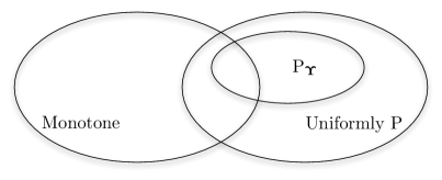
Figure 1: Relation among NEP classes.

Figure 1 summarizes the relations between these classes of problems. Note that a monotone NEP is not necessarily uniformly P; it is enough to observe that monotone NEPs may have multiple NE (see Example #1 in Sec. 7), whereas uniformly P NEPs have only one solution [cf. Theorem 3(d)]. Similarly, $P{}_{\boldsymbol{\Upsilon}}$ NEPs (and thus uniformly P NEPs) are not a subclass of monotone NEPs, as shown by the following example.

Example 9 (A P_Υ NEP which is not monotone)

Consider a real NEP with two players, each controlling one scalar variable: $x_{1}$ and $x_{2}$. The players’ problems are

$$\begin{array}[]{rl}{\displaystyle{\hbox{minimize}_{x_{1}}}}&\dfrac{1}{2}x_{1}^{2}+4x_{1}x_{2}\\[5.0pt] {\mathrm{s}ubject\,to}&x_{1}\,\in\,[0,10]\end{array}\qquad\qquad\begin{array}[]{rl}{\displaystyle{\hbox{minimize}_{x_{2}}}}&\dfrac{1}{2}x_{2}^{2}-\dfrac{1}{8}x_{1}x_{2}\\[5.0pt] \hbox{subject\, to\,}&x_{2}\,\in\,[-2,2]\end{array}\vspace{-.1cm}$$

The VI associated to this NEP is VI$([0,10]\times[-2,2],\mathbf{F})$, with $\mathbf{F}=[x_{1}+4x_{2},x_{2}-(1/8)x_{1}]^{T}$. The symmetric part of $\mathbf{J}\mathbf{F}$, $\mathbf{J}\mathbf{F}_{s}$, and the matrix $\boldsymbol{\Upsilon}_{\mathbf{F}}$ are given by:

$$\mathbf{J}\mathbf{F}_{s}\,=\,\left[\begin{array}[]{cc}1&31/16\\ 31/16&1\end{array}\right],\qquad\qquad\boldsymbol{\Upsilon}_{\mathbf{F}}\,=\,\left[\begin{array}[]{cc}1&-4\\ -1/8&1\end{array}\right].$$

Since $\mathbf{J}\mathbf{F}_{s}$ has a negative determinant, $\mathbf{F}$ cannot be monotone; on the other hand it is easy to check that the two principal minors of $\boldsymbol{\Upsilon}_{\mathbf{F}}$ are positive, implying that $\mathcal{G}$ is a P NEP.

Centralized algorithms for monotone and uniformly $P{}_{\boldsymbol{\Upsilon}}$ NEPs, based on VI theory, are well-known [31, vol II]; in this paper, we focus on the more challenging issue of devising distributed (and possibly asynchronous) solution schemes for NEPs, which is the topic of the next section.

4 Distributed Algorithms for NEPs

This section along with the next one constitute the core theoretical part of the paper. We develop here a novel theory that allows devising distributed algorithms for computing Nash equilibria in several significant settings. More specifically, we will provide novel distributed (asynchronous) algorithms for the solution of: (a) $P{}_{\boldsymbol{\Upsilon}}$ NEPs; and (b) monotone NEPs.

Since monotone NEPs may have multiple solutions, in case (a) we will further consider both the situations in which one is interested in computing any one solution, and the situations in which one wants to select the best solution, according to a given criterion. In each of the settings above we will provide best-response-based distributed algorithms along with their convergence properties; the proposed algorithms differ in: i) the computational effort; ii) the players’ synchronization/signaling requirements; and iii) the convergence speed. Note that while centralized solution methods are known for uniformly P NEPs, the development of distributed algorithms for this class of games is at the time of this writing an open problem.

This section is organized in three parts. Sec. 4.1 and Sec. 4.2 focus on algorithms for $P{}_{\boldsymbol{\Upsilon}}$ and monotone NEPs, respectively; results in this sections will be the building blocks for the more difficult issue of equilibrium selection problem addressed in Sec. 4.3.

4.1 Best-response distributed algorithms for $P{}_{\boldsymbol{\Upsilon}}$ NEPs

Since in a NEP every player is trying to minimize his own objective function, a natural approach to compute a solution of a NEP is to consider an iterative algorithm wherein all the players, given the strategies of the others and according to a given scheduling (e.g., sequentially or simultaneously), update their own strategy by solving their optimization problem (12). Here, we focus on a very general class of best-response-based algorithms, namely the totally asynchronous best-response algorithms (in the sense specified in [45]). In these schemes, some players may update their strategies more frequently than others and they may even use an outdated information about the strategy profile used by the others; which is very appealing in many practical multiuser communication systems, such as wireless ad-hoc networks or CR systems wherein synchronization requirements are hard to enforce.

To provide a formal description of the algorithm, we need to introduce some preliminary definitions. In an asynchronous scheme, the users may not update their own strategies at each iteration; let denote then by $\mathcal{T}_{i}\subseteq\mathcal{T}\subseteq\left\{0,1,2,\ldots\right\}$ the set of times at which player $i$ updates his own strategy $\mathbf{x}_{i}$, denoted by $\mathbf{x}_{i}^{(n)}$ (thus, implying that, at time $n\notin\mathcal{T}_{i}$, $\mathbf{x}_{i}^{(n)}$ is left unchanged). Moreover, in computing their optimal strategy, the users can use an outdated version of the others’ strategies; let then $\tau_{j}^{i}(n)$ be the most recent time at which the strategy profile of player $j$ is perceived by player $i$ at the $n$-$th$ iteration (observe that $\tau_{j}^{i}(n)$ satisfies $0\leq\tau_{j}^{i}(n)\leq n$). Hence, if player $i$ updates its strategy at the $n$-th iteration, then he minimizes his cost function using the following (possibly) outdated strategy profile of the other players:

$$\mathbf{x}_{-i}^{(\mathbf{\boldsymbol{{\tau}}}^{i}(n))}\triangleq\left(\mathbf{x}_{1}^{(\tau_{1}^{i}(n))},\ldots,\mathbf{x}_{i-1}^{(\tau_{i-1}^{i}(n))},\mathbf{x}_{i+1}^{(\tau_{i+1}^{i}(n))},\ldots,\mathbf{x}_{I}^{(\tau_{I}^{i}(n))}\right).$$ (19)

Some standard conditions in asynchronous convergence theory, which are fulfilled in any practical implementation, need to be satisfied by the schedule $\mathcal{T}_{i}$’s and $\tau_{j}^{i}(n)$’s, namely for each $i$:

A1)

$0\leq\tau_{j}^{i}(n)\leq n$ (at any given iteration $n$, each player $i$ can use only the strategy profile $\mathbf{x}_{-i}^{(\mathbf{\tau}^{i}(n))}$ adopted by the other players in the previous iterations );

A2)

$\lim_{k\rightarrow\infty}\tau_{j}^{i}(n_{k})=+\infty$, where $\{n_{k}\}$ is a sequence of elements in $\mathcal{T}_{i}$ that tends to infinity [for any given iteration index $n_{k}$, the values of the components of $\mathbf{x}_{-i}^{(\mathbf{\tau}^{i}(n))}$ in (19) generated prior to $n_{k}$ are not used in the updates of $\mathbf{x}_{i}^{(n)}$, when $n$ becomes sufficiently larger than $n_{k}$];

A3)

$\left|\mathcal{T}_{i}\right|=\infty$ (no player fails to update his own strategy as time $n$ goes on).

Using the above definitions, the totally asynchronous algorithm based on the best-responses of the players is described in Algorithm 20. The convergence properties of the algorithm are given in Theorem 10.

 Algorithm 1: Asynchronous Best-Response Algorithm

 $\mbox{(\mbox{S.0})}:$ Choose any feasible $\mathbf{x}^{(0)}\in\mathcal{Q}$ and set $n=0$.

$\mbox{(S.1)}:$ If $\mathbf{x}^{(n)}$ satisfies a suitable termination criterion: STOP

$\mbox{(S.2)}:$ for $i=1,\ldots,I$, compute

$$\mathbf{x}_{i}^{(n+1)}=\left\{\begin{array}[]{lll}\mathbf{x}_{i}^{\star}\in\underset{\mathbf{x}_{i}\in\mathcal{Q}_{i}}{\text{{argmin}}}f_{i}\left(\mathbf{x}_{i},\,\mathbf{x}_{-i}^{(\boldsymbol{{\tau}}^{i}(n))}\right),&&\mbox{if }n\in\mathcal{T}_{i}\vskip 6.0pt plus 2.0pt minus 2.0pt\\ \mathbf{x}_{i}^{(n)},&&\mbox{otherwise}\end{array}\right.$$ (20)

$\mbox{(S.3)}:$ $n\leftarrow n+1$; go to (S.1).

 

Theorem 10

Let $\mathcal{G}=\left\langle\mathcal{Q},\,\mathbf{f}\right\rangle$ be a $P{}_{\boldsymbol{\Upsilon}}$ NEP. Any sequence $\{\mathbf{x}^{(n)}\}_{n=0}^{\infty}$ generated by Algorithm 20 converges to the unique NE of ${\mathcal{G}}$, for any given updating schedule of the players satisfying assumptions A1-A3.

Proof. See Appendix C.  

Remark 11 (Flexibility of the algorithm)

Algorithm 20 contains as special cases a large number of algorithms, each one obtained by a possible choice of the schedule of the users in the updating procedure (i.e., the parameters $\{\tau_{j}^{i}(n)\}$ and $\{\mathcal{T}_{i}\}$). Examples are the simultaneous (Jacobi scheme) and sequential (Gauss-Seidel scheme) updates, where the players update their own strategies simultaneously and sequentially, respectively. Indeed, the Jacobi update corresponds to the schedule $\tau_{j}^{i}(n)=n$ and $\mathcal{T}_{i}=\{1,2,\ldots\}$ for all $i$ and $j$, whereas the Gauss-Seidel scheme is obtained by taking $\tau_{j}^{i}(n)=n$ and $\mathcal{T}_{i}=\{i,\,i+I,\,i+2I,\ldots\}$ for all $i$ and $j$. Moreover, variations of such a totally asynchronous scheme, e.g., including constraints on the maximum tolerable delay in the updating and on the use of the outdated information (which leads to the so-called partially asynchronous algorithms), can also be considered [45]. An important result stated in Theorem 10 is that all the algorithms resulting as special cases of Algorithm 20 are guaranteed to reach the unique NE of the NEP, under the same set of convergence conditions, since the matrix $\boldsymbol{{\Upsilon}}_{\mathbf{F}}$ does not depend on the particular choice of $\{\tau_{j}^{i}(n)\}$ and $\{\mathcal{T}_{i}\}$. Note that all the algorithms coming from Algorithm 20 are robust against missing or outdated updates of the players. This feature strongly relaxes the constraints on the synchronization of the players’ updates; which makes this class of algorithms appealing in many practical distributed systems.

Note that the (synchronous) projection-response algorithms for monotone VIs (and thus NEPs) proposed in [35] and [31, 34] are not guaranteed to converge if applied to a P_Υ NEP that is not monotone. $\square$

Remark 12 (On the convergence conditions)

Global convergence of Algorithm 20 is guaranteed under the P property of $\boldsymbol{\Upsilon}_{\mathbf{F}}$ (or equivalently $\rho(\boldsymbol{\Gamma}_{\mathbf{F}})<1$). However, we have already pointed out in Remark 6 that such a condition cannot be satisfied if there is a player whose cost function has a singular Hessian, even in just one point. In fact, if this is the case, we have, $\alpha_{i}^{\min}=0$ for some $i$, let us say $i=1$, which implies that $\boldsymbol{\Gamma}_{\mathbf{F}}$ has a 1 in the left-upper corner. Since $\boldsymbol{\Gamma}_{\mathbf{F}}$ is nonnegative, we have that this implies $\rho(\boldsymbol{\Gamma_{\mathbf{F}}})\geq 1$ [46, Th. 1.7..4]. Assuming that the element 1 is contained in an irreducible principal matrix, we will actually have $\rho(\boldsymbol{\Gamma_{\mathbf{F}}})>1$. Note that the irreducibility assumption is extremely weak and trivially satisfied if $\boldsymbol{\Gamma_{\mathbf{F}}}$ is positive, which is true in many applications. In the next section we discuss a remedy for this issue. $\square$

Remark 13 (On the convergence rate)

As shown in Proposition 42 in Appendix C, in the setting of Theorem 10 the best-response mapping [see (95)] is a contraction. Building on this and choosing for notational simplicity in (16) $\mathbf{C}_{i}=\mathbf{I}$ for all $i$, it is straightforward to show that the convergence rate of the synchronous Jacobi version of Algorithm 20 is geometric with factor $\left\|\boldsymbol{{\Gamma_{\mathbf{F}}}}\right\|<1$ (see, e.g., [45, Prop. 1.1]). Therefore, one can readily determine how many iterations are needed to surely achieve a desired accuracy $\varepsilon>0$:

$$\left\|\mathbf{x}^{n}-\mathbf{x}^{\star}\right\|\leq\varepsilon\quad\mbox{for}\,\,\mbox{any}\,\,\mbox{positive}\,\,n\geq\overline{{n}}\triangleq\log\left(\dfrac{{\varepsilon\,\left(1-\left\|\boldsymbol{{\Gamma_{\mathbf{F}}}}\right\|\right)}}{\left\|\mathbf{x}^{(1)}-\mathbf{x}^{(0)}\right\|}\right)/\log\left(\left\|\boldsymbol{{\Gamma_{\mathbf{F}}}}\right\|\right),$$ (21)

where $\mathbf{x}^{\star}$ is the unique NE of $\mathcal{G}$ and $\left\|\boldsymbol{{\Gamma_{\mathbf{F}}}}\right\|<1$ is the best-response contraction constant, with $\boldsymbol{{\Gamma_{\mathbf{F}}}}$ defined in (15). Note that when the joint feasible set $\mathcal{Q}$ is bounded with diameter $d_{\mathcal{Q}}$, we can obtain an overestimate of $\overline{{n}}$ that is independent on $\mathbf{x}^{(1)}$ and $\mathbf{x}^{(2)}$: $\overline{{n}}\leq\log\left({\varepsilon\,\left(1-\left\|\boldsymbol{{\Gamma_{\mathbf{F}}}}\right\|\right)}/d_{\mathcal{Q}}\right)/\log\left(\left\|\boldsymbol{{\Gamma_{\mathbf{F}}}}\right\|\right)$.

The case of asynchronous implementations is conceptually similar but necessarily more complex; we refer the interested reader to [45, Sec. 6.3.5]. $\square$

4.2 Proximal distributed algorithms for monotone NEPs

In this section we deal with monotone NEPs (see Definition 8). Since monotone NEPs in general have multiple NE, Algorithm 20 solving $P{}_{\boldsymbol{\Upsilon}}$ (or uniformly P) NEPs may fail to converge. There is a host of solution methods available in the literature to solve monotone real VIs and thus monotone NEPs (see, e.g., [31, Vol. II]), but these algorithms are centralized. Recently, in [35], the authors proposed some distributed synchronous schemes for solving monotone VIs, based on the gradient-response mapping; we have already discussed the main drawbacks of these algorithms, see Sec. 1 (see also Sec. 6 for some numerical results).

The development of distributed best-response algorithms for solving monotone NEPs with (possibly) multiple solutions is a challenging task; in this subsection, we cope with this issue building on a regularization technique known as proximal algorithms, see [31, Ch 12] for an introduction to proximal point methods for VIs. The proposed approach is to reduce the solution of a single monotone NEP to the solution of a sequence of $P{}_{\boldsymbol{\Upsilon}}$ NEPs with a particular structure. The advantage of this method is that we can efficiently solve each of the $P{}_{\boldsymbol{\Upsilon}}$ NEPs with convergence guarantee using Algorithm 1 (cf. Sec. 4.1); the disadvantage is that, to recover the solution of the original monotone NEP, one has to solve a (possibly infinite) number of $P{}_{\boldsymbol{\Upsilon}}$ NEPs. However, it is important to remark from the outset that this potential drawback is greatly mitigated by the fact that, as we discuss shortly, (i) one only needs to solve these $P{}_{\boldsymbol{\Upsilon}}$ NEPs inaccurately; (ii) the (inaccurate) solution of the $P{}_{\boldsymbol{\Upsilon}}$ NEPs usually requires little computational effort; and (iii) in practice, a fairly accurate solution of the original NEP is obtained after solving a limited number of $P{}_{\boldsymbol{\Upsilon}}$ NEPs.

Before introducing the formal description of the algorithm, let us begin with some simple observations motivating how the sequence of $P{}_{\boldsymbol{\Upsilon}}$ NEPs is built. Let $\mathcal{G}=\left\langle\mathcal{Q},\mathbf{f}\right\rangle$ be a monotone NEP; consider a perturbation of this game defined as $\mathcal{G}_{\tau,\mathbf{y}}=\left\langle\mathcal{Q},\,(f_{i}+(\tau/2)\|\bullet-\mathbf{y}_{i}\|^{2})_{i=1}^{I}\right\rangle$, where $\tau$ is a positive parameter and $\mathbf{y}=(\mathbf{y}_{i})_{i=1}^{I}$ is a given vector in $\mathbb{R}^{n}$, with each $\mathbf{y}_{i}\in\mathbb{R}^{n_{i}}$; we term $\mathbf{y}$ center of the regularization. Note that $\mathcal{G}_{\tau,\mathbf{y}}$ is the game wherein each player $i$, anticipating $\mathbf{x}_{-i}\in\mathcal{Q}_{-i}$, solves the following convex optimization problem:

$$\begin{array}[]{ll}\mathop{\mathrm{m}inimize}\limits_{\mathbf{x}_{i}}&f_{i}(\mathbf{x}_{i},\,\mathbf{x}_{-i})+\frac{\tau}{2}\|\mathbf{x}_{i}-\mathbf{y}_{i}\|^{2}\\[5.0pt] \text{subject to}&\mathbf{x}_{i}\in{\cal Q}_{i}.\end{array}$$ (22)

Let us consider now the VI reformulations of $\mathcal{G}$ and $\mathcal{G}_{\tau,\mathbf{y}}$, given by $\mathop{\mathrm{V}I}(\mathcal{Q},\mathbf{F})$ and $\mathop{\mathrm{V}I}(\mathcal{Q},\mathbf{F}_{\tau,\mathbf{y}})$ respectively, where $\mathbf{F}(\mathbf{x})\triangleq\left(\nabla_{\mathbf{x}_{i}}f_{i}(\mathbf{x})\right)_{i=1}^{I}$ and $\mathbf{F}_{\tau,\mathbf{y}}(\mathbf{x})=\mathbf{F}(\mathbf{x})+\tau\,(\mathbf{x}-\mathbf{y})$, and let us introduce the matrices $\boldsymbol{\Upsilon}_{\mathbf{F}}$ and $\boldsymbol{\Upsilon}_{\mathbf{F}_{\tau,\mathbf{y}}}$ associated to $\mathcal{G}$ and $\mathcal{G}_{\tau,\mathbf{y}}$, respectively [see (15)]. It is not difficult to check that

$$\boldsymbol{\Upsilon}_{\mathbf{F}_{\tau,\mathbf{y}}}=\boldsymbol{\Upsilon}_{\mathbf{F}}+\tau\mathbf{I}.\vspace{-0.1cm}$$ (23)

Note that $\boldsymbol{\Upsilon}_{\mathbf{F}_{\tau,\mathbf{y}}}$ does not depend on $\mathbf{y}$. It follows readily from (23) that if $\tau$ is large enough, $\Upsilon_{\mathbf{F}_{\tau,\mathbf{y}}}$ is a P matrix, meaning that $\mathcal{G}_{\tau,\mathbf{y}}$ is a $P{}_{\boldsymbol{\Upsilon}}$ NEP, for any given $\mathbf{y}\in\mathbb{\mathbb{R}}^{n}$. More specifically, using the definitions of $\beta_{ij}^{\max}$’s and $\alpha_{i}^{\min}$’s as given in (16), we have the following.

Lemma 14

For any given $\mathbf{y}\in\mathbb{R}^{n}$, the game $\mathcal{G}_{\tau,\mathbf{y}}=\left\langle\mathcal{Q},\,(f_{i}+(\tau/2)\cdot\right.$ $\left.\|\bullet-\mathbf{y}_{i}\|^{2})_{i=1}^{I}\right\rangle$ is a $P{}_{\boldsymbol{\Upsilon}}$ NEP for every $\tau$ larger than $\bar{\tau}$ (independent of $\mathbf{y}$), with

$$\bar{\tau}\triangleq\max_{1\leq i\leq I}\left\{\sum_{j\neq i}\beta_{ij}^{\max}-\alpha_{i}^{\min}\right\}.$$ (24)

Nice as it is, the result above would be of no practical interest if we were not able to connect the solutions of $\mathcal{G}_{\tau,\mathbf{y}}$ to those of $\mathcal{G}$. Indeed, the solutions of $\mathcal{G}$ and $\mathcal{G}_{\tau,\mathbf{y}}$ are in general different but, nevertheless, there exists a connection between them: a point $\mathbf{x}^{\star}$ is a solution of $\mathcal{G}$ if and only if $\mathbf{x}^{\star}$ is a solution of $\mathcal{G}_{\tau,\mathbf{x}^{\star}}$.

Proposition 15

Let $\mathcal{G}=\left\langle\mathcal{Q},\mathbf{f}\right\rangle$ be a monotone NEP. For any given $\tau>0$, $\mathbf{x}^{\star}\in\mathcal{Q}$ is a solution of $\mathcal{G}$ if and only if $\mathbf{x}^{\star}$ is a solution of $\mathcal{G}_{\tau,\mathbf{x}^{\star}}$.

Proof. See Appendix D. 

Lemma 14 and Proposition 15 open the way to the design of convergent distributed algorithms for monotone NEPs, as shown next. Let us choose $\tau$ being large enough so that $\mathcal{G}_{\tau,\mathbf{y}}$ is a $P{}_{\boldsymbol{\Upsilon}}$ NEP (cf. Lemma 14). It follows from Theorem 3 that $\mathcal{G}_{\tau,\mathbf{y}}$ has a unique solution, denoted by $\mathbf{S}_{\tau}(\mathbf{y})$. Using $\mathbf{S}_{\tau}(\mathbf{y})$, Proposition 15 can be restated as follows: $\mathbf{x}^{\star}$ is a solution of $\mathcal{G}$ if and only if it is a fixed point of $\mathbf{S}_{\tau}(\mathbf{\bullet})$, i.e., $\mathbf{x}^{\star}=\mathbf{S}_{\tau}(\mathbf{x}^{\star})$. It seems then natural to compute the solutions of $\mathcal{G}$ using the fixed-point-type iteration $\mathbf{x}^{(n+1)}=\mathbf{S}_{\tau}(\mathbf{\mathbf{x}}^{(n)})$, starting from a feasible point $\mathbf{x}^{(0)}$; which corresponds to solving the sequence of NEPs $\mathcal{G}_{\tau,\mathbf{x}^{(n)}}$ for $n=0,1,\ldots$. If $\tau$ is sufficiently large [e.g., as in (24)], each $\mathcal{G}_{\tau,\mathbf{x}^{(n)}}$ is a $P{}_{\boldsymbol{\Upsilon}}$ NEP (cf. Lemma 14), and thus its unique solution can be computed in a distributed way with convergence guarantee by the asynchronous best-response algorithm described in Algorithm 20 (cf. Theorem 10). The above discussion motivates the following algorithm for computing the solutions of a monotone NEP, whose convergence properties are given in Theorem 16 below.

 Algorithm 2: Proximal Decomposition Algorithm (PDA)

 $\textbf{Data}:$ Let $\tau>0$ be given.

$\mbox{(\mbox{S.0})}:$ Choose any feasible $\mathbf{x}^{(0)}\in\mathcal{Q}$ and set $n=0$.

$\mbox{(S.1)}:$ If $\mathbf{x}^{(n)}$ satisfies a suitable termination criterion: STOP.

$\mbox{(S.2)}:$ Solve the game $\mathcal{G}_{\tau,\mathbf{x}^{(n)}}$ and set $\mathbf{x}^{(n+1)}\triangleq\mathbf{S}_{\tau}(\mathbf{x}^{(n)})$

$\mbox{(S.3)}:$ $n\leftarrow n+1$; go to $\mbox{(S.1)}.$

 

Theorem 16

Let $\mathcal{G}=\left\langle\mathcal{Q},\,\mathbf{f}\right\rangle$ be a monotone NEP with a nonempty solution set. Suppose that $\tau$ is large enough so that $\boldsymbol{\Upsilon}_{\mathbf{F}_{\tau,\,\mathbf{y}}}$ is a P matrix. Then, Algorithm 4.2 is well defined, and the sequence $\{\mathbf{x}^{(n)}\}_{n=0}^{\infty}$ generated by the algorithm converges to a solution of the game $\mathcal{G}$.

Algorithm 4.2 is of great conceptual interest, but its applicability is limited, unless one is able to easily compute $\mathbf{S}_{\tau}(\mathbf{x}^{(n)})$. Although there are interesting problems in which this can be done efficiently (see Sec. 6), in general one is expected to solve a number of $P{}_{\boldsymbol{\Upsilon}}$ NEPs, each of them requiring an infinite iterative method to compute each $\mathbf{S}_{\tau}(\mathbf{x}^{(n)})$. To overcome this issue, we propose next a variant of Algorithm 4.2, in which suitable approximations of $\mathbf{S}_{\tau}(\mathbf{x}^{(n)})$ can be used. Algorithm 4.2 below describes such a variant, where we have added a further degree of freedom in the updating rule: the new iteration $\mathbf{x}^{(n+1)}$ is not necessarily given by (an approximation of) $\mathbf{S}_{\tau}(\mathbf{x}^{(n)})$, but lies instead on the line connecting the old iteration $\mathbf{x}^{(n)}$ to (the approximation of) $\mathbf{S}_{\tau}(\mathbf{x}^{(n)})$.

 Algorithm 3: Approximate Proximal Decomposition Algorithm (APDA)

 $\textbf{Data}:$ Let $\{\varepsilon^{(n)}\}_{n=0}^{\infty}$, $\{\eta^{(n)}\}_{n=0}^{\infty}$ and $\tau>0$ be given.

$\mbox{(\mbox{S.0})}:$ Choose any feasible $\mathbf{x}^{(0)}\in\mathcal{Q}$ and set $n=0$.

$\mbox{(S.1)}:$ If $\mathbf{x}^{(n)}$ satisfies a suitable termination criterion: STOP.

$\mbox{(S.2)}:$ Solve the game $\mathcal{G}_{\tau,\mathbf{x}^{(n)}}$ within the accuracy $\varepsilon^{(n)}$: Find a $\mathbf{z}^{(n)}$ s.t. $\|\mathbf{z}^{(n)}-\mathbf{S}_{\tau}(\mathbf{x}^{(n)})\|\leq\varepsilon^{(n)}$.

$\mbox{(S.3)}:$ Set $\mathbf{x}^{(n+1)}\triangleq(1-\eta^{(n)})\mathbf{x}^{(n)}+\eta^{(n)}\mathbf{z}^{(n)}$.

$\mbox{(S.4)}:$ $n\leftarrow n+1$; go to $\mbox{(S.1)}.$

 

The error term $\varepsilon^{(n)}$ measures the accuracy used at iteration $n$ in computing the solution $\mathbf{S}_{\tau}(\mathbf{x}^{(n)})$ of $\mathcal{G}_{\tau,\mathbf{x}^{(n)}}$. The parameter $\eta^{(n)}$ instead, introduces a memory in the updating rule, it establishes where exactly we move along the line passing through the old iterations $\mathbf{x}^{(n)}$ and $\mathbf{z}^{(n)}$. Note that if we take $\varepsilon^{(n)}=0$ and $\eta^{(n)}=1$ for all $n$, Algorithm 4.2 reduces to Algorithm 4.2. The advantage of Algorithm 4.2 with respect to Algorithm 4.2 is that $\mathbf{z}^{(n)}$ can be computed in a finite number of steps, so that Algorithm 4.2 becomes implementable in practice. Obviously, the errors $\varepsilon^{(n)}$’s and the parameters $\eta^{(n)}$’s must be chosen according to some suitable conditions, if one wants to guarantee convergence. These conditions are established in the following theorem.

Theorem 17

Let $\mathcal{G}=\left\langle\mathcal{Q},\,\mathbf{f}\right\rangle$ be a monotone NEP with a nonempty solution set. Suppose that $\tau$ is large enough so that $\boldsymbol{\Upsilon}_{\mathbf{F}_{\tau,\,\mathbf{y}}}$ is a P-matrix. Choose $\{\varepsilon^{(n)}\}\subset[0,\infty)$ such that $\sum_{n=1}^{\infty}\varepsilon^{(n)}<\infty$ and $\{\eta^{(n)}\}\subset[R_{m},R_{M}]$, with $0<R_{m}\leq R_{M}<2$. Then, Algorithm 4.2 is well defined, and the sequence $\{\mathbf{x}^{(n)}\}_{n=0}^{\infty}$ generated by the algorithm converges to a solution of $\mathcal{G}$.

The proof of Theorem 17 (and thus also Theorem 16) is a consequence of the following facts and thus is omitted: i) [31, Th. 12..3.9]; ii) The observation that $\mathcal{G}$ is equivalent to the VI$(\mathcal{Q},\mathbf{F})$ (Proposition 2), with $\mathbf{F}=(\nabla_{\mathbf{x}_{i}}f_{i})_{i=1}^{I}$, and the VI$(\mathcal{Q},\mathbf{F})$ has a solution; and iii) Under the P property of $\boldsymbol{\Upsilon}_{\mathbf{F}_{\tau,\,\mathbf{y}}}$, Step S.2 of Algorithm 4.2 (and Algorithm 4.2) is well defined (Theorem 10).

It is interesting to remark that for sake of simplicity we assumed $\tau$ to be a fixed number. However, $\tau$ can be varied from iteration to iteration provided that $\tau\in(\bar{{\tau}},\tau^{\max}]$, where $\tau^{\max}$ is any finite number. We also note that the sequence $\{\mathbf{x}^{(n)}\}$ generated by Algorithm 4.2 may not be feasible, but all the limit points are feasible. If one is interested in maintaining feasibility throughout the iterates, it is enough to choose $\eta^{(n)}\leq 1$ and compute in Step 2 a feasible $\mathbf{z}^{(n)}$, which can be done, e.g., by applying Algorithm 20 to $\mathcal{G}_{\tau,\mathbf{x}^{(n)}}$.

While the utility of having possibly inexact solutions in Step S.2 of Algorithm 4.2 is apparent, the usefulness of Step S.3 is less evident. This kind of “averaging” is known as over-relaxation and has its roots in classical successive over-relaxation methods for solving systems of linear equations [47, Sec. 7.4]. In our context, the extra degree of freedom offered by Step S.3 can bring numerical improvements; see, e.g., [31].

Algorithm 4.2 is conceptually a double loop scheme wherein at each (outer) iteration $n$, given $\mathbf{x}^{(n)}$, one needs to compute the approximation $\mathbf{z}^{(n)}$, which requires an inner iterative process. Since the condition $\sum_{n=1}^{\infty}\varepsilon^{(n)}<\infty$ implies $\varepsilon^{(n)}\downarrow 0$, when the iterations progress, $\mathbf{S}_{\tau}(\mathbf{x}^{(n)})$ has to be estimated with an increasing accuracy. However, in practice, this is not a problem since when iterations progress, $\{\mathbf{x}^{(n)}\}$ usually converges, implying $\|\mathbf{x}^{(n+1)}-\mathbf{x}^{(n)}\|\to 0$. One can then use $\mathbf{x}^{(n)}$ as a good approximation to initialize any (inner) procedure in Step 2 to compute $\mathbf{z}^{(n)}$. It turns out that, in spite of the increasing precision requirements, in practice a suitable $\mathbf{z}^{(n)}$ in Step 2 can be computed very easily.

Finally, observe that a natural choice for computing $\mathbf{z}^{(n)}$ in Step 2 of Algorithm 4.2 is Algorithm 20. When this choice is made, Algorithm 4.2 also becomes an asynchronous method, having all the desired features described in the previous section (see Remark 11). The only difference with Algorithm 20 is that, in Algorithm 4.2, “from time to time” (precisely when the inner termination test $\|\mathbf{z}^{(n)}-\mathbf{S}_{\tau}(\mathbf{x}^{(n)})\|\leq\varepsilon^{(n)}$ in Step 2 is satisfied) the objective function of the players are changed by updating the regularizing term from $\frac{\tau}{2}\|\mathbf{x}_{i}-\mathbf{x}_{i}^{(n)}\|^{2}$ to $\frac{\tau}{2}\|\mathbf{x}_{i}-\mathbf{x}_{i}^{(n+1)}\|^{2}$, which generally requires some coordination among the players to establish when a satisfactory approximation $\mathbf{z}^{(n)}$ has been reached. The remark below discusses issues related to this aspect.

Remark 18 (On the inner termination criterion)

We have seen that, in Step 2 of Algorithm 4.2, the players must be able to decide whether $\|\mathbf{z}^{(n)}-\mathbf{S}_{\tau}(\mathbf{x}^{(n)})\|\,\leq\,\varepsilon^{(n)}$ holds. This can be easily done if one uses a synchronous Jacobi version of Algorithm 20; in fact one can readily estimate the number of iterations needed to achieve the accuracy $\varepsilon^{(n)}$ using (21), where $\boldsymbol{{\Gamma}}_{\mathbf{F}}$ is replaced by $\boldsymbol{{\Gamma}}_{\mathbf{F}_{\tau}}$. However, this estimate can be very conservative and, in any case, it is not applicable if an asynchronous version of Algorithm 20 is used. In the following we suggest a different, simple, distributed protocol to decide whether $\|\mathbf{z}^{(n)}-\mathbf{S}_{\tau}(\mathbf{x}^{(n)})\|\,\leq\,\varepsilon^{(n)}$, which can be used in both synchronous and asynchronous implementations of Algorithm 20.

Observe preliminarily that an error bound on the distance of the current iteration $\mathbf{z}^{(n)}$ from the solution $\mathbf{S}_{\tau}(\mathbf{x}^{(n)})$ of $\mathcal{G}_{\tau,\mathbf{x}^{(n)}}$ can be obtained by solving a convex (quadratic) problem (see, e.g., [31, Prop. 6.3.1], [31, Prop. 6.3.7]). For example, under the P properties of $\boldsymbol{\Upsilon}_{\mathbf{F}_{\tau,\mathbf{x}^{(n)}}}$ defined in (23), the following error bound holds for the game $\mathcal{G}_{\tau,\mathbf{x}^{(n)}}$ [31, Prop. 6.3.1]: a (finite) constant $c>0$ exists such that

$$\|\mathbf{z}-\mathbf{S}_{\tau}(\mathbf{x}^{(n)})\|\,\leq c\,\|\mathbf{F}_{\tau}^{\text{\emph{nat}}}\left(\mathbf{z}\right)\|,\quad\forall\mathbf{z}\in\mathcal{Q},$$ (25)

where $\mathbf{F}_{\tau}^{\text{{nat}}}\left(\mathbf{z}\right)\triangleq\mathbf{z}-\Pi_{\mathcal{Q}}\left(\mathbf{z}-\mathbf{F}(\mathbf{z})-\tau\,\mathbf{z}\right)$, with $\Pi_{\mathcal{Q}}\left(\mathbf{x}\right)$ denoting the Euclidean projection of $\mathbf{x}$ onto the closed and convex set $\mathcal{Q}$. Note that, since $\mathcal{Q}$ has a Cartesian structure, $\mathbf{F}_{\tau}^{\text{{nat}}}\left(\mathbf{z}\right)$ can be partitioned as $\mathbf{F}_{\tau}^{\text{{nat}}}\left(\mathbf{z}\right)=\left(\left[\mathbf{F}_{\tau}^{\text{{nat}}}\left(\mathbf{z}\right)\right]_{i}\right)_{i=1}^{I}$, where each $\left[\mathbf{F}_{\tau}^{\text{{nat}}}\left(\mathbf{z}\right)\right]_{i}=\mathbf{z}_{i}-\Pi_{\mathcal{Q}_{i}}\left(\mathbf{z}_{i}-\mathbf{F}_{i}(\mathbf{z})-\tau\,\mathbf{z}_{i}\right)$ can be locally computed by the associated player $i$ by solving a quadratic program, as long as $\mathbf{F}_{i}(\mathbf{z})$ is available at the player side.

Using (25), the implementation of Step 2 of Algorithm 4.2 can be obtained as follows. Each player $i$ choses preliminarily a suitable local termination sequence $\{\varepsilon_{i}^{(n)}\}_{n}\subset[0,\infty)$ such that $\sum_{n=1}^{\infty}\varepsilon_{i}^{(n)}<\infty$; the termination criterion of each player $i$ becomes then $\left\|\left[\mathbf{F}_{\tau}^{\text{{nat}}}\left(\mathbf{x}^{(n)}\right)\right]_{i}\right\|\leq\varepsilon_{i}^{(n)}$, which can be locally implemented. Once the desired local accuracy is reached by all the players, they can all update the center of their regularization. Note that this protocol guarantees that the requirement on the sequence $\varepsilon^{(n)}$ in Step 2 as stated in Theorem 17 is met, since $\varepsilon^{(n)}\triangleq\sum_{i=1}^{I}\varepsilon_{i}^{(n)}$ satisfies $\sum_{n=1}^{\infty}\varepsilon^{(n)}<\infty$. $\square$

Remark 19 (On the communications overhead)

The last issue to address for a practical implementation of the termination protocols discussed in Remark 18 is how the players can detect the others having reached the desired accuracy in Step 2 of Algorithm 4.2. If one uses a synchronous Jacobi version of Algorithm 20 in Step 2 and the joint feasible set $\mathcal{Q}$ is bounded, conceptually there is no need of any information exchange, since each player can locally estimate the number of iterations needed to reach the accuracy $\varepsilon^{(n)}$ as discussed in Remark 13. However, even when possible, this approach is probably too conservative, since the estimated $\overline{{n}}$ can be unnecessarily large. In practice, and whenever one is not using a synchronous Jacobi method, the termination criterion (25) can be easily implemented, at the cost of limited signaling, performing the following protocol. Each user sends out one bit when $\left\|\left[\mathbf{F}_{\tau}^{\text{{nat}}}\left(\mathbf{x}^{(n)}\right)\right]_{i}\right\|\leq\varepsilon_{i}^{(n)}$. Once one and therefore all players receive bits from all the others, they can update their regularization. Note that in the context of distributed algorithms for the solution of optimization problems, VIs, and games, this is a minimal signaling requirement; see, e.g., [48, 49] and [45, Ch. 1.3, 1.4], [45, Ch. 3.5.7], [45, Ch. 8] for some representative examples. Furthermore, we observe that in many practical applications exchanging one bit is viable. For instance, in the CR systems considered in Sec. 2 and Sec. 6, this can be done using network control channels.

Finally, we conclude this remark suggesting a simple heuristic that does not require any signaling: each user updates its regularization only after experiencing no changes in $\left\|\left[\mathbf{F}_{\tau}^{\text{{nat}}}\left(\mathbf{x}^{(n)}\right)\right]_{i}\right\|$ (or his cost function) for a prescribed number of iterations. While this heuristic does not guarantee theoretical convergence, its effectiveness in many practical scenarios, as those considered in Sec. 6, is rather apparent. $\square$

4.3 Equilibrium selection for monotone NEPs

In the previous section we discussed distributed algorithms for the computation of a solution of monotone NEPs. A feature of these algorithms is that they converge under mild conditions that do not imply the uniqueness of the NE of the NEP. In the presence of multiple equilibria, however, the proposed algorithms do not allow to perform any selection of the solution they reach, but they may converge in principle to any NE of the game; which makes the achievable system performance unpredictable. It would be interesting instead to be able to select, among all the solutions of the game, the one(s) that satisfies some additional criterion. We refer to this problem as equilibrium selection problem. In this section, we address this issue; the outcome will be a novel set of distributed algorithms along with their convergence properties that solve the equilibrium selection problem; this additional feature comes at the price of a (moderate) increase of the complexity in computing the players’ best-response solution and signaling among the players.

Let us introduce first an informal description of the algorithm. Let $\mathcal{G}=<\mathcal{Q},\,\mathbf{f}>$ be a monotone NEP and let $\mathop{\mathrm{S}OL}(\mathcal{Q},\,\mathbf{f})$ denote its solution set, assumed to be nonempty without loss of generality. Recall that since $\mathcal{G}$ is monotone, $\mathop{\mathrm{S}OL}(\mathcal{Q},\,\mathbf{f})$ is always convex (cf. Theorem 3). Stated in mathematical terms, the equilibrium selection problem consists in solving the following bi-level optimization problem:

$$\begin{array}[]{ll}\mathop{\mathrm{m}inimize}\limits_{\mathbf{x}}&\phi(\mathbf{x})\\[5.0pt] \text{subject to}&\mathbf{x}\in\mathop{\mathrm{S}OL}(\mathcal{Q},\,\mathbf{f}),\end{array}\vskip 6.0pt plus 2.0pt minus 2.0pt\vspace{-0.2cm}$$ (26)

where the function $\phi:\mathbb{R}^{n}\rightarrow\mathbb{R}$ is assumed to be continuously differentiable and convex. The function $\phi$ thus defines the additional criterion according to which one wants to select a solution in the set of the NE of $\mathcal{G}$: solving (26) indeed corresponds to choosing the NE of $\mathcal{G}$ that minimizes $\phi$. Note that, under the monotonicity of $\mathcal{G}$, (26) is a convex optimization problem [$\mathop{\mathrm{S}OL}(\mathcal{Q},\,\mathbf{f})$ is convex]. However, standard solution techniques cannot be applied because the feasible set $\mathop{\mathrm{S}OL}(\mathcal{K},\mathbf{f})$ is only implicitly defined and, in general, it is not expressed as a standard system of inequalities. To overcome this difficulty, and in the same spirit of the previous section, instead of attacking problem (26) directly, we propose to solve a sequence of standard regularized NEPs (“standard” means a game whose players’ feasible sets are not of an implicit type, and therefore can be solved by classic methods, like Algorithm 20). Each standard regularized game has the following structure $\mathcal{G}_{\tau,\varepsilon,\mathbf{y}}=\left\langle\mathcal{Q},\,(f_{i}+\varepsilon\,\phi+(\tau/2)\|\bullet-\mathbf{y}_{i}\|^{2})_{i=1}^{I}\right\rangle$, where $\varepsilon$ and $\tau$ are fixed positive constants and $\mathbf{y}\triangleq(\mathbf{y}_{i})_{i=1}^{I}$ is a given point in $\mathbb{R}^{n}$ with each $\mathbf{y}_{i}\in\mathbb{R}^{n_{i}}$; $\mathcal{G}_{\tau,\varepsilon,\mathbf{y}}$ is a NEP wherein each player $i$, anticipating $\mathbf{x}_{-i}\in\mathcal{Q}_{-i}$, solves the following convex optimization problem:

$$\begin{array}[]{ll}\mathop{\mathrm{m}inimize}\limits_{\mathbf{x}_{i}}&f_{i}(\mathbf{x}_{i},\,\mathbf{x}_{-i})+\varepsilon\,\phi(\mathbf{x}_{i},\,\mathbf{x}_{-i})+\frac{\tau}{2}\|\mathbf{x}_{i}-\mathbf{y}_{i}\|^{2}\\[5.0pt] \text{subject to}&\mathbf{x}_{i}\in{\cal Q}_{i}.\end{array}$$ (27)

Note that the players’ problems in this game differ from (22) in the presence of the additional term $\varepsilon\phi(\mathbf{x})$ in the objective function. It is not surprising that $\phi$ appears in the players’ objective functions; roughly speaking, it represents the additional amount of information to be included in the game to “drive” the system toward the desired solution.

Proceeding as in the previous section, we can now establish the connection between the regularized NEPs $\mathcal{G}_{\tau,\varepsilon,\mathbf{y}}$ and the equilibrium selection problem (26). Fist of all note that, in the setting of problem (26), the NEPs $\mathcal{G}_{\tau,\varepsilon,\mathbf{y}}$ is equivalent to the VI$(\mathcal{Q},\mathbf{F}_{\tau,\varepsilon,\mathbf{y}})$ where $\mathbf{F}_{\tau,\varepsilon,\mathbf{y}}\triangleq\mathbf{F}+\varepsilon\,\nabla\phi+\tau\,(\mathbf{I}-\mathbf{y})$ and $\mathbf{I}:\mathbf{x}\mapsto\mathbf{x}$ is the identity map. Denoting by $\boldsymbol{\Upsilon}_{\mathbf{F}_{\tau,\varepsilon,\mathbf{y}}}$ the matrix defined in (15) and associated to $\mathbf{F}_{\tau,\varepsilon,\mathbf{y}}$, Lemma 20 below shows that there exists a sufficiently large $\tau$ such that $\boldsymbol{\Upsilon}_{\mathbf{F}_{\tau,\varepsilon,\mathbf{y}}}$ is a P matrix, implying that $\mathcal{G}_{\tau,\varepsilon,\mathbf{y}}$ is a $P{}_{\boldsymbol{\Upsilon}}$ NEP.

Lemma 20

Let $\mathcal{G}=\left\langle\mathcal{Q},\,\mathbf{f}\right\rangle$ be a monotone NEP; let $\phi:\mathbb{R}^{n}\mapsto\mathbb{R}$ be a continuously differentiable function on $\mathcal{Q}$ whose gradient $\nabla\phi$ is Lipschitz continuous on $\mathcal{Q}$, with constant $L_{\phi}$; and let $\bar{\varepsilon}>0$ be given. For any fixed $\mathbf{y}\in\mathbb{R}^{n}$, the game $\mathcal{G}_{\tau,\varepsilon,\mathbf{y}}=\left\langle\mathcal{Q},\,(f_{i}+\varepsilon\phi+(\tau/2)\|\bullet-\mathbf{y}_{i}\|^{2})_{i=1}^{I}\right\rangle$ with $\varepsilon\in[0,\bar{\varepsilon}]$ is a $P{}_{\boldsymbol{\Upsilon}}$ NEP for every $\tau$ larger than $\bar{\tau}_{\bar{\varepsilon}}$ (independent on $\mathbf{y}$ and $\varepsilon$)

$$\bar{\tau}_{\bar{\varepsilon}}\triangleq\max_{1\leq i\leq I}\left\{\sum_{j\neq i}\beta_{ij}^{\max}-\alpha_{i}^{\min}\right\}+(I-1)\,\bar{\varepsilon}\,L_{\phi},\vspace{-0.2cm}$$ (28)

where $\beta_{ij}^{\max}$’s and $\alpha_{i}^{\min}$’s are defined in (16).

In the setting of Lemma 20, $\mathcal{G}_{\tau,\varepsilon,\mathbf{y}}$ is a $P{}_{\boldsymbol{\Upsilon}}$ NEP and thus has a unique solution, denoted by $\mathbf{S}_{\tau,\varepsilon}(\mathbf{y})$ [cf. Theorem 3]; such a $\mathbf{S}_{\tau,\varepsilon}(\mathbf{y})$ can be computed with convergence guaranteed using Algorithm 20 on $\mathcal{G}_{\tau,\varepsilon,\mathbf{y}}$. The solution of the original equilibrium selection problem (26) can be recovered using the fixed-point-type iteration $\mathbf{x}^{(n+1)}=\mathbf{S}_{\tau,\varepsilon^{(n)}}(\mathbf{\mathbf{x}}^{(n)})$, starting from a feasible point $\mathbf{x}^{(0)}$ and by suitably varying $\varepsilon^{(n)}$; which corresponds to solve the sequence of NEPs $\mathcal{G}_{\tau,\varepsilon^{(n)},\mathbf{x}^{(n)}}$ for $n=0,1,\ldots$. This procedure is made formal in Algorithm 4.3 below.

 Algorithm 4: Proximal-Tikhonov Regularization Algorithm (PTRA)

 $\textbf{Data}:$ Let $\{\varepsilon^{(n)}\}\downarrow 0$ and $\tau>0$ be given.

$\mbox{(\mbox{S.0})}:$ Choose any feasible $\mathbf{x}^{(0)}\in\mathcal{Q}$ and set $n=0$.

$\mbox{(\mbox{S.1})}:$ If $\mathbf{x}^{(n)}$ satisfies a suitable termination criterion, STOP.

$\mbox{(\mbox{S.2})}:$ Set $\mathbf{x}^{(n+1)}$ to be the solution of the game $\mathcal{G}_{\tau,\varepsilon^{(n)},\mathbf{x}^{(n)}}$.

$\mbox{(\mbox{S.3})}:$ Set $n\leftarrow n+1$ and return to (S.1).

 

Note that, since in Algorithm 4.3 the sequence $\{\varepsilon^{(n)}\}$ converges to zero, there always exists an $\bar{\varepsilon}>0$ such that $\varepsilon^{(n)}\in[0,\bar{\varepsilon}]$, implying by Lemma 20 that for a sufficiently large $\tau$ all the games $\mathcal{G}_{\tau,\varepsilon^{(n)},\mathbf{x}^{(n)}}$ in the Step 2 of the algorithm are $P{}_{\boldsymbol{\Upsilon}}$ NEPs and thus have a unique solution; this makes the sequence $\{\mathbf{x}^{(n)}\}_{n=0}^{\infty}$ generated by Algorithm 4.3 well defined. The convergence properties of the algorithm are given in the following theorem.

Theorem 21

Let $\mathcal{G}=\left\langle\mathcal{Q},\,\mathbf{f}\right\rangle$ be a monotone NEP with a nonempty solution set $\mathop{\mathrm{S}OL}(\mathcal{Q},\,\mathbf{f})$. Consider the equilibrium selection problem (26) and suppose that i) $\phi$ is continuously differentiable and convex on $\mathcal{Q}$; ii) the level sets of $\phi$ on $\mathop{\mathrm{S}OL}(\mathcal{Q},\,\mathbf{f})$ are bounded; and iii) $\nabla\phi$ is Lipschitz continuous on $\mathcal{Q}$, with constant $L_{\phi}$. Moreover, suppose that $\tau$ is large enough so that $\mathcal{G}_{\tau,\varepsilon^{(n)},\mathbf{x}^{(n)}}$ is a $P{}_{\boldsymbol{\Upsilon}}$ NEP for any $n$, and choose the sequence $\{\varepsilon^{(n)}\}$ such that $\varepsilon^{(n)}>0$ for all $n$, $\{\varepsilon^{(n)}\}\downarrow 0$, and $\sum_{n=0}^{\infty}\,\varepsilon^{(n)}=\infty$. Then Algorithm 4.3 is well defined; the sequence $\{\mathbf{x}^{(n)}\}_{n=0}^{\infty}$ is bounded; and every of its limit points is a solution of (26).

Proof. See Appendix E.  

Theorem 21 guarantees convergence of the algorithm under mild assumptions. Conditions on $\phi$ are pretty standard; in particular, assumptions i) and ii) together with the monotonicity of $\mathcal{G}$ state that the optimization problem (26) is convex and admits a solution; whereas iii) guarantees that there exists a finite (large enough) $\tau$ such that $\mathcal{G}_{\tau,\varepsilon^{(n)},\mathbf{x}^{(n)}}$ is a $P{}_{\boldsymbol{\Upsilon}}$ NEP (cf. Lemma 20). The assumptions on the sequence $\{\varepsilon^{(n)}\}_{n=1}^{\infty}$ are also rather weak and require $\varepsilon^{(n)}$ to go to zero, but not too fast; which can be satisfied, e.g., by taking $\varepsilon^{(n)}=1/(1+na)$, with $n=0,1,2,\ldots$ and $a$ being any positive constant. This assumption on $\varepsilon^{(n)}$ is not new and has already been used in a few papers dealing with the combination of Tikhonov and proximal regularization; we refer the reader to [50] and references therein for a wider discussion on this point.

The implementation of Algorithm 4.3 requires the ability of solving at each round $n$ the $P{}_{\boldsymbol{\Upsilon}}$ NEP $\mathcal{G}_{\tau,\varepsilon^{(n)},\mathbf{x}^{(n)}}$. If one is interested in distributed solution schemes, Algorithm 20 applied to $\mathcal{G}_{\tau,\varepsilon^{(n)},\mathbf{x}^{(n)}}$ is the natural choice. Note that the convergence conditions of the algorithm applied to $\mathcal{G}_{\tau,\varepsilon^{(n)},\mathbf{x}^{(n)}}$ as stated in Theorem 10 are always met, provided $\tau$ is large enough; see, e.g., (28) in Lemma 20.

As in the previous section, note that, unless one has simple ways to compute the solutions of the games $\mathcal{G}_{\tau,\varepsilon^{(n)},\mathbf{x}^{(n)}}$, Algorithm 4.3 requires at each step the exact computation of the solution of the regularized games $\mathcal{G}_{\tau,\varepsilon^{(n)},\mathbf{x}^{(n)}}$ (inner loop), which in principle requires a conceptually infinite procedure. While in practice this might not be a problem, it still leaves open the question of whether, paralleling the results of the previous section, one can develop versions of Algorithm 4.3 where inexact solutions are used in the Step 2. The answer to this question is positive, but the corresponding theory is rather complex and, for sake of simplicity, we prefer to omit it here; the interest reader can work it out using results in [21].

4.4 A bird’s-eye view

In the previous three sections we proposed several distributed algorithms for real player-convex NEPs, which are applicable to different scenarios. Fig. 2 summarizes the results obtained so far, showing that, in spite of apparent diversities, all the algorithms belong to a same family.

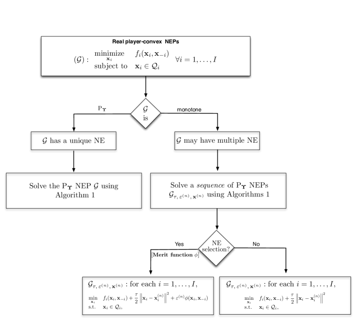
Figure 2: The roadmap of the proposed distributed solution methods for real player-convex NEPs

Conceptually, what we have proposed is indeed a unified algorithm, where the users can explicitly choose the degree of desired cooperation and signaling, converging to solutions having different performance, namely: i) any one NE, when there is no (or very limited) cooperation among users, and ii) the “best” NE (according to an outer merit function $\phi$), at the cost of more coordination. The choice of one scheme in favor to the other as well as the merit function $\phi$ will depend then on the trade-off between signaling and performance that the users are willing to exchange/achieve. The core of the proposed solution methods can be summarized in the following unified updating rule: at iteration $n$, the optimal strategy of each user $i$ is

$$\mathbf{x}_{i}^{(n+1)}=\underset{\mathbf{x}_{i}\in\mathcal{Q}_{i}}{\text{argmin}}\left\{f_{i}\left(\mathbf{x}_{i},\mathbf{x}_{-i}^{(n)}\right)+\pi_{i}^{(\nu_{n})}\left(\mathbf{x}_{i},\,\mathbf{x}_{-i}^{(n)}\right)+\dfrac{\tau}{2}\,\left\|\mathbf{x}_{i}-\mathbf{x}_{i}^{(\nu_{n})}\right\|^{2}\right\}$$ (29)

where the first term $f_{i}(\mathbf{x}_{i},\mathbf{x}_{-i}^{(n)})$ is the usual term in an iterative best-response algorithm, the second term $\pi_{i}^{(\nu_{n})}(\mathbf{x}_{i},\,\mathbf{x}_{-i}^{(n)})$ (whose update is performed at iteration $\nu_{n}$) can be interpreted as a nonlinear pricing in the objective function of the users, and the third term $\dfrac{\tau}{2}\,\left\|\mathbf{x}_{i}-\mathbf{x}_{i}^{(\nu_{n})}\right\|^{2}$ is a (proximal) regularization. Observe that there are two iteration indexes: $n$ is the main discrete-time unit, whereas $\nu_{n}$ is increased every few discrete-time units (e.g., if $\nu_{n}=\left\lfloor n/10\right\rfloor$, then $\nu_{n}$ is updated every 10 discrete-time units).

The price function $\pi_{i}^{(\nu_{n})}$ can be interpreted as a measure of the “altruism/selfishness” of the users and represents the trade-off factor between signaling and performance. Indeed, we may have the following:

• $\pi_{i}^{(\nu_{n})}=0$ (no cooperation): The users are not willing to cooperate; the best one can get is converge to any one solution of the game (i.e., with no control on the quality of the solution); this is guaranteed even in the presence of multiple equilibria if the NEP is monotone ($P{}_{\boldsymbol{\Upsilon}}$);

• $\pi_{i}^{(\nu_{n})}\neq 0$ (some cooperation): The users may exchange some signaling in the form of pricing through the function $\pi_{i}^{(\nu_{n})}(\mathbf{x}_{i},\,\mathbf{x}_{-i}^{(n)})=\varepsilon^{(\nu_{n})}\,\phi(\mathbf{x}_{i},\,\mathbf{x}_{-i}^{(n)})$ and converge to the NE that minimizes the merit function $\phi(\mathbf{x})$; convergence is guaranteed if the NEP is monotone.

Remark 22 (Role of pricing)

It is important to remark that the pricing term $\pi_{i}^{(\nu_{n})}$ does not need to be linear; moreover it has a well understood role in the system optimization. This is a major departure from current literature that uses linear pricing as a heuristic to improve the performance of a NE in power control games (see, e.g., [51] for scalar power control problems); in these works there is neither a proof of convergence of the modified game nor a theoretical explanation of the performance improvement due to pricing. As a direct product of our framework, we obtain instead a clear understanding of the meaning of the pricing; for example, a linear price in the form $\varepsilon^{(\nu_{n})}\,\boldsymbol{{\pi}}_{i}^{T}\mathbf{x}_{i}$, with $\varepsilon^{(\nu_{n})}\rightarrow 0$, corresponds to the selection of a NE that minimizes the linear function $\sum_{i}\boldsymbol{{\pi}}_{i}^{T}\mathbf{x}_{i}$, resulting likely in better system performance.

5 Variational Inequalities and Games in the Complex Domain

The results presented so far apply to real NEPs. However, in many applications, e.g., in digital communications, array processing, and signal processing, the variables involved in the optimization are complex. For instance, in the MIMO problems introduced in Sec. 2, players’ optimization variables are complex matrices. For these applications the reformulation of the problem into the real domain is awkward, very difficult to handle, and generally leads to final conditions that cannot be easily interpreted in terms of the original complex setup. Indeed, this “natural” approach has long been abandoned in the signal processing and communication communities, since it has shown to be inadequate. It seems instead more convenient to work directly in the complex domain. This requires the use of some sophisticated tools hinging on involved analytic developments. However, once one has mastered these tools, the prize is a very smooth and immediate generalization of all the results developed in the previous section, thus easily providing a whole set of new methods for the solution of NEPs in the complex domain.

In order to follow this plan in this section we first recall some basic results about the so-called Wirtinger calculus, prompted by the lack of a well-established notation and definitions for $\mathbb{R}$-matrix derivatives; two good tutorials on the subject are [52, 53]. We then proceed to the development of several new technical tools that are then applied to the study of VIs and NEPs in the complex domain. We start introducing in Sec. 5.2 the minimum principle for constrained convex optimization problems in the domain of complex matrices, generalizing the already known complex gradient-vanishing conditions obtained in [52] for the unconstrained case. As intermediate result, we also introduce a Taylor expansion of real-valued functions of complex matrices that is amenable to our MIMO applications. The second important contribution is given in Sec. 5.3, where, after introducing the VI problem in the complex domain and the associated monotonicity and P properties, we provide new matrix conditions for these properties to hold. These conditions are the natural generalization of those obtained in Sec. 3, provided that a new definition of Jacobian matrix for complex-valued matrix functions as well as a tailored concept of positive (semi-)definiteness are used. Finally, in Sec. 5.5, we establish the connection between VIs and NEPs in the complex domain, and discuss its main implications.

5.1 $\mathbb{R}$-matrix derivatives

In practical applications, we often deal with optimization of real-valued functions $f:\mathbb{C}\ni z\mapsto f(z)\in\mathbb{R}$ of a complex variable $z$ that are not differentiable in $\mathbb{C}$ (termed also $\mathbb{C}$-differentiable or holomorphic). However, the same univariate function $f:\mathbb{C}\rightarrow\mathbb{R}$ can also be viewed as a bivariate function of its real and imaginary components, i.e., $f(z)=g(z_{R},z_{I})$, where $g:\mathbb{R}^{2}\mapsto\mathbb{R}$ is a real-valued function of the real variables $z_{R}\triangleq\text{{Re}}(z)$ and $z_{I}\triangleq\text{{Im}}(z)$. This way, one may be able to replace the nonexistence of the $\mathbb{C}$-derivative of $f$ with the existence of the real partial derivatives of $g(z_{R},z_{I})$, which is actually what one needs to compute a stationary point of the function. This motivates the introduction of the so-called $\mathbb{R}$-derivative and conjugate $\mathbb{R}$-derivative of $f:\mathbb{C}\rightarrow\mathbb{R}$ at $z_{0}\in\mathbb{C}$, formally defined as

$$\frac{{\partial}f}{\partial z}(z_{0})\triangleq\dfrac{{1}}{2}\,\left.\left(\frac{{\partial}f(z)}{\partial z_{R}}-j\frac{{\partial}f(z)}{\partial z_{I}}\right)\right|_{z=z_{0}}\quad\mbox{and}\quad\frac{{\partial}f}{\partial z^{\ast}}(z_{0})\triangleq\dfrac{{1}}{2}\,\left.\left(\frac{{\partial}f(z)}{\partial z_{R}}+j\frac{{\partial}f(z)}{\partial z_{I}}\right)\right|_{z=z_{0}},$$ (30)

respectively, where $j=\sqrt{{-1}}$. Note that the derivatives above must be interpreted formally, because $z$ and its conjugate $z^{\ast}$ in (30) are treated as they were mutually independent; the derivatives $\frac{{\partial}f}{\partial z_{R}}$ and $\frac{{\partial}f}{\partial z_{I}}$ represent instead the true (non-formal) partial derivatives of $f$ viewed as a bivariate function of $z_{R}$ and $z_{I}$, i.e., $f=\check{f}(z_{R},z_{I})$. When $\frac{{\partial}f}{\partial z_{R}}$ and $\frac{{\partial}f}{\partial z_{I}}$ exist (and are continuous), implying that (30) is well-defined, we say that $f$ is $\mathbb{R}$-differentiable (or continuously $\mathbb{R}$-differentiable); similarly to the real case, when we say that a function $f:\mathcal{K}\rightarrow\mathbb{R}$ is $\mathbb{R}$-differentiable (or continuously $\mathbb{R}$-differentiable) on the closed set $\mathcal{K}$, we mean that the function is so on an open set containing $\mathcal{K}$.

The $\mathbb{R}$-derivatives defined in (30) for a real-valued function can be naturally extended to complex-valued functions of a complex argument, that is, $f:\mathbb{C}\rightarrow\mathbb{C}$; formally we still have (30), but now $f(z)=\check{f}(z_{R},z_{I})\triangleq\check{f}_{R}(z_{R},z_{I})+j\cdot\check{f}_{I}(z_{R},z_{I})$, with $\check{f}:\mathbb{R}^{2}\mapsto\mathbb{C}$ and $\check{f}_{R},\check{f}_{I}:\mathbb{R}^{2}\mapsto\mathbb{R}$, and by ${\partial}f/\partial z_{R}$ we mean ${\partial}f/\partial z_{R}\triangleq{\partial}\check{f}_{R}/{\partial}z_{R}+j\cdot{\partial}\check{f}_{I}/{\partial}z_{R}$ (similarly for ${\partial}f/\partial z_{I}$).

When $f$ is a (complex-valued) scalar function of complex matrices, that is $f:\mathbb{C}^{n\times m}\rightarrow\mathbb{C}$, we have $n\cdot m$ component-wise $\mathbb{R}$-derivatives $\frac{{\partial}f}{\partial\left(\mathbf{Z}\right)_{ij}}$ and $n\cdot m$ conjugate $\mathbb{R}$-derivatives $\frac{{\partial}f}{\partial\left(\mathbf{Z}^{\ast}\right)_{ij}}$. The question naturally arises how to order these $n\cdot m$ complex terms; obviously this can be done in many ways. It is worthwhile noticing that, even though they all contain the same $n\cdot m$ derivatives, not all definitions have the same properties; for instance for some of them a useful chain rule does not exist. Next, we introduce two definitions, both useful for our derivations and widely used in the literature [52]; in the former definition, the $n\cdot m$ (conjugate) $\mathbb{R}$-derivatives are displayed in the same order as $(\mathbf{Z})_{ij}$ and $(\mathbf{Z}^{\ast})_{ij}$ appear in $\mathbf{Z}$ and $\mathbf{Z}^{\ast}$, whereas in the latter we arrange all the elements in a row vector. Given $f:\mathbb{C}^{n\times m}\rightarrow\mathbb{C}$, the (matrix) gradient and co(njugate)-gradient of $f$ at $\mathbf{Z}_{0}\in\mathbb{C}^{n\times m}$ are defined as

$$\begin{array}[]{l}\,\,\nabla_{\mathbf{Z}}f(\mathbf{Z}_{0})\triangleq\left.\dfrac{{\partial}\,f(\mathbf{Z})}{\partial\mathbf{Z}}\right|_{\mathbf{Z}=\mathbf{Z}_{0}}\quad\mbox{with}\quad\left[\dfrac{{\partial}\,f}{\partial\mathbf{Z}}\right]_{ij}=\dfrac{{\partial}\,f}{\partial\,(\mathbf{Z})_{ij}},\quad\,\,\,\forall i=1,\ldots,n\quad\mbox{and}\quad j=1,\dots,m\vskip 12.0pt plus 4.0pt minus 4.0pt\\ \nabla_{\mathbf{\mathbf{Z}^{\ast}}}f(\mathbf{Z}_{0})\triangleq\left.\dfrac{{\partial}f(\mathbf{Z})}{\partial\mathbf{Z^{\ast}}}\right|_{\mathbf{Z}=\mathbf{Z}_{0}}\quad\mbox{with}\quad\left[\dfrac{{\partial}\,f}{\partial\mathbf{Z}^{\ast}}\right]_{ij}=\dfrac{{\partial}\,f}{\partial\,(\mathbf{Z}^{\ast})_{ij}},\quad\forall i=1,\ldots,n\quad\mbox{and}\quad j=1,\dots,m,\end{array}$$ (31)

where $\frac{{\partial}f}{\partial(\mathbf{Z})_{ij}}$ and $\frac{{\partial}f}{\partial(\mathbf{Z})_{ij}^{\ast}}$ are the $\mathbb{R}$-derivative and conjugate $\mathbb{R}$-derivative of the complex-valued function $f$ w.r.t. $\left(\mathbf{Z}\right)_{ij}$ and $\left(\mathbf{Z}^{\ast}\right)_{ij}$, respectively. Note that $\nabla_{\mathbf{Z}}f(\mathbf{Z}_{0})$ and $\nabla_{\mathbf{Z}^{\ast}}f(\mathbf{Z}_{0})$ are matrices having the same size of $\mathbf{Z}$. Alternatively, one can arrange the elements $\frac{{\partial}f}{\partial(\mathbf{Z})_{ij}}$ and $\frac{{\partial}f}{\partial(\mathbf{Z}^{\ast})_{ij}}$ in a row vector, and define $D_{\mathbf{Z}}f(\mathbf{Z})$ and $D_{\mathbf{Z^{\ast}}}f(\mathbf{Z})$ at $\mathbf{Z}_{0}\in\mathbb{C}^{n\times m}$ as

$$\begin{array}[]{l}D_{\mathbf{Z}}f(\mathbf{Z}_{0})\triangleq\left.\dfrac{{\partial}\,f(\mathbf{Z})}{\partial\,\text{{vec}}\left(\mathbf{Z}\right)^{T}}\right|_{\mathbf{Z}=\mathbf{Z}_{0}}=\text{{vec}}\left(\nabla_{\mathbf{Z}}f(\mathbf{Z}_{0})\right)^{T}\,\,\mbox{and\,}\,\,D_{\mathbf{Z}^{\ast}}f(\mathbf{Z}_{0})\triangleq\left.\dfrac{{\partial}\,f(\mathbf{Z})}{\partial\,\text{{vec}}\left(\mathbf{Z}^{\ast}\right)^{T}}\right|_{\mathbf{Z}=\mathbf{Z}_{0}}=\text{{vec}}\left(\nabla_{\mathbf{Z}^{\ast}}f(\mathbf{Z}_{0})\right)^{T}\end{array},$$ (32)

where $\text{{vec}}\left(\mathbf{A}\right)^{T}$ stands for $\left(\text{{vec}}\left(\mathbf{A}\right)\right)^{T}$. For (complex-valued) matrix functions of complex matrices, $\mathbf{F}^{\mathbb{C}}:\mathbb{C}^{n\times m}\rightarrow\mathbb{C}^{p\times q}$, we arrange the $pq\cdot nm$ (conjugate) $\mathbb{R}$-derivatives in the following $pq\times nm$ matrices

$$\begin{array}[]{c}D_{\mathbf{Z}}\mathbf{F}^{\mathbb{C}}(\mathbf{Z}_{0})\triangleq\left.\dfrac{{\partial}\,\text{{vec}}\left(\mathbf{F}^{\mathbb{C}}(\mathbf{Z})\right)}{\partial\,\text{{vec}}\left(\mathbf{Z}\right)^{T}}\right|_{\mathbf{Z}=\mathbf{Z}_{0}},\,\,\mbox{with}\,\,\left[\dfrac{{\partial}\,\text{{vec}}\left(\mathbf{F}^{\mathbb{C}}\right)}{\partial\,\text{{vec}}\left(\mathbf{Z}\right)^{T}}\right]_{ij}=\dfrac{{\partial}\,\left[\text{{vec}}\left(\mathbf{F}^{\mathbb{C}}\right)\right]_{i}}{\partial\,\left[\text{{vec}}\left(\mathbf{Z}\right)\right]_{j}},\,\,\forall i=1,\ldots,pq\,\,\mbox{and}\,\,j=1,\dots,nm,\vskip 12.0pt plus 4.0pt minus 4.0pt\\ D_{\mathbf{Z}^{\ast}}\mathbf{F}^{\mathbb{C}}(\mathbf{Z}_{0})\triangleq\left.\dfrac{{\partial}\,\text{{vec}}\left(\mathbf{F}^{\mathbb{C}}(\mathbf{Z})\right)}{\partial\,\text{{vec}}\left(\mathbf{Z}^{\ast}\right)^{T}}\right|_{\mathbf{Z}=\mathbf{Z}_{0}},\,\,\mbox{with}\,\,\left[\dfrac{{\partial}\,\text{{vec}}\left(\mathbf{F}^{\mathbb{C}}\right)}{\partial\,\text{{vec}}\left(\mathbf{Z}^{\ast}\right)^{T}}\right]_{ij}=\dfrac{{\partial}\,\left[\text{{vec}}\left(\mathbf{F}^{\mathbb{C}}\right)\right]_{i}}{\partial\,\left[\text{{vec}}\left(\mathbf{Z}^{\ast}\right)\right]_{j}},\,\,\forall i=1,\ldots,pq\,\,\mbox{and}\,\,j=1,\dots,nm.\end{array}$$ (33)

The $pq\times nm$ matrices $D_{\mathbf{Z}}\mathbf{F}^{\mathbb{C}}$ and $D_{\mathbf{Z}^{\ast}}\mathbf{F}^{\mathbb{C}}$ are called Jacobian and conjugate Jacobian of $\mathbf{F}^{\mathbb{C}}$. Note that when $\mathbf{F}^{\mathbb{C}}$ is a scalar function of $\mathbf{Z}$, i.e., $\mathbf{F}^{\mathbb{C}}(\mathbf{Z})=f(\mathbf{Z})$ with $f:\mathbb{C}^{n\times m}\rightarrow\mathbb{C}$, definitions (33) reduce to (32). Practical rules to compute $\mathbb{R}$-derivatives and conjugate $\mathbb{R}$-derivatives introduced above can be found in [52].

5.2 The minimum principle

Let $\mathbb{C}^{n\times m}$ be the space of complex $n\times m$ matrices, and let $\mathcal{K}\subseteq\mathbb{C}^{n\times m}$ be a closed and convex set. We consider the optimization problem

$$\begin{array}[]{ll}\mathop{\mathrm{m}inimize}\limits_{\mathbf{Z}}&f(\mathbf{Z})\\[5.0pt] \text{subject to}&\mathbf{Z}\in\mathcal{K},\end{array}$$ (34)

where $f:\mathcal{K}\rightarrow\mathbb{R}$ is a real-valued convex and continuously $\mathbb{R}$-differentiable function on $\mathcal{K}$. At the basis of the minimum principle there is the first-order Taylor expansion of $f$ at $\mathbf{Z}_{0}\in\mathcal{K}$ as proved in Appendix F:

$$f(\mathbf{\mathbf{Z}_{0}}+\Delta\mathbf{Z})-f(\mathbf{Z}_{0})\simeq \,\text{2\,\text{{Re}}$\left(\,\text{{tr}}\left(\left(\nabla_{\mathbf{Z}}f(\mathbf{Z}_{0})\right)^{T}\Delta\mathbf{Z}\right)\,\right)$}\triangleq 2\,\left\langle\Delta\mathbf{Z},\,\nabla_{\mathbf{Z}^{\ast}}f(\mathbf{Z}_{0})\right\rangle$$ (35)

where we used $\left(\nabla_{\mathbf{Z}}f\right)^{\ast}=\nabla_{\mathbf{\mathbf{Z}^{\ast}}}f$ since $f$ is real [see (30)], and we introduced the inner product $\left\langle\bullet,\,\bullet\right\rangle:\mathbb{C}^{n\times n}\times\mathbb{C}^{n\times n}\rightarrow\mathbb{R}$, defined as

$$\left\langle\mathbf{A},\,\mathbf{B}\right\rangle\triangleq\text{{Re}}\left(\,\text{{tr}}\left(\mathbf{A}^{H}\mathbf{B}\right)\,\right).$$ (36)

Note that the norm induced by the inner product $\left\langle\bullet,\,\bullet\right\rangle$ is the Frobenius norm, i.e., $\left\langle\mathbf{A},\,\mathbf{A}\right\rangle=\text{Tr}(\mathbf{A}^{H}\mathbf{A})=\left\|\mathbf{A}\right\|_{F}^{2}.$ Using (35) we can now introduce the minimum principle as given next.

Lemma 23

Given the convex optimization problem (34) in the setting above, $\mathbf{X}\in\mathcal{K}$ is an optimal solution of (34) if and only if $\mathbf{X}$ satisfies $\left\langle\mathbf{Z}-\mathbf{X},\,\nabla_{\mathbf{Z}^{\ast}}f\mathbf{(X)}\right\rangle\geq 0$ for all $\mathbf{Z}\in\mathcal{K}$.

Proof. See Appendix F. 

It is interesting to observe that if the optimal solution $\mathbf{X}$ is in the interior of $\mathcal{K}$ [e.g., the optimization problem (34) is unconstrained, implying $\mathcal{K}=\mathbb{C}^{n\times m}$), then the above optimality conditions reduce to $\nabla_{\mathbf{Z}^{\ast}}f\mathbf{(X)}=\mathbf{0}$, or equivalently $\nabla_{\mathbf{Z}}f\mathbf{(X)}=\mathbf{0}$, which are the well-established complex gradient-vanishing conditions obtained in [52] for the unconstrained minimization. We conclude this section with an example of application of the minimum principle, which is instrumental for the analysis in Sec. 6.

Example 24 (An application of the minimum principle)

Consider the following single-user rate maximization problem

$$\begin{array}[]{ll}\mathop{\mathrm{m}aximize}\limits_{\mathbf{Z}}&f(\mathbf{Z})\triangleq\log\det\left(\mathbf{R}_{n}+\mathbf{H}\mathbf{Z}\mathbf{H}^{H}\right)\\[5.0pt] \text{subject to}&\mathbf{Z}\in\mathcal{K},\end{array}$$ (37)

where $\mathbf{R}_{n}\in\mathbb{C}^{m\times m}$ is a positive definite matrix, $\mathbf{H}\in\mathbb{C}^{m\times n}$, and $\mathcal{K}$ is any convex and compact subset of the $n\times n$ complex positive semidefinite matrices (assumed to be nonempty). Note that $f(\mathbf{Z})$ is a concave (real-valued) function on the feasible set $\mathcal{K}$ but is not real if defined on $\mathbb{C}^{n\times n}$. Since we are interested in minimizing $f$ over $\mathcal{K}$, in order to apply the minimum principle, one approach we can follow is to consider without loss of generality the modified function $\tilde{f}:\widetilde{\mathcal{K}}\rightarrow\mathbb{R}$, defined as $\tilde{f}(\mathbf{Z})\triangleq 2\,\text{{Re}}\left(f(\mathbf{Z})\right)$, where $\mathcal{K}\subset\widetilde{\mathcal{K}}\subseteq\mathbb{C}^{n\times n}$ is any open set over which $f(\mathbf{Z})$ is well defined (it is sufficient that $\det\left(\mathbf{R}_{n}+\mathbf{H}\mathbf{Z}\mathbf{H}^{H}\right)\neq 0$); indeed, $\tilde{f}$ coincides with $f$ over $\mathcal{K}$, but it is real everywhere (in its domain). Moreover, $\tilde{f}$ is $\mathbb{R}$-differentiable on $\widetilde{\mathcal{K}}$. The conjugate (matrix) $\mathbb{R}$-derivative of $\tilde{f}$ at $\mathbf{Z}_{0}\in\widetilde{\mathcal{K}}$ is (see Appendix G)

$$\nabla_{\mathbf{\mathbf{Z}^{\ast}}}\tilde{{f}}(\mathbf{Z}_{0})=\mathbf{H}^{H}(\mathbf{R}_{n}+\mathbf{H}\mathbf{Z}_{0}^{H}\mathbf{H}^{H})^{-1}\mathbf{H}.$$ (38)

Introducing $\mathbf{G}:\mathcal{K}\rightarrow\mathbb{C}^{n\times n}$, defined as $\mathbf{G}=\mathbf{G}(\mathbf{Z})\triangleq-\nabla_{\mathbf{\mathbf{Z}^{\ast}}}\tilde{f}(\mathbf{Z})=-\mathbf{H}^{H}(\mathbf{R}_{n}+\mathbf{H}\mathbf{Z}\mathbf{H}^{H})^{-1}\mathbf{H}$ (note that $\mathbf{Z}\in\mathcal{K}$ and thus $\mathbf{Z}=\mathbf{Z}^{H}$), and invoking Lemma 23, the optimization problem (37) is then equivalent to the minimum principle: find a $\mathbf{Z}\in\mathcal{K}$ such that $\left\langle\mathbf{Y}-\mathbf{Z},\,\mathbf{G}(\mathbf{Z})\right\rangle\geq 0$, for all $\mathbf{Y}\in\mathcal{K}$. $\square$

5.3 The VI problem in the complex domain

With the developments of the previous section at hand, we can now introduce the definition of the VI problem in the domain of complex matrices, termed the complex VI problem. Similarly to the real case (cf. Appendix A), one can think of the VI problem as the generalization of the minimum principle (cf. Lemma 23), where the co-gradient $\nabla_{\mathbf{Z}^{\ast}}f$ is replaced with a complex-valued matrix mapping. The formal definition is given next.

Definition 25

Given a convex and closed set $\mathcal{K}\subseteq\mathbb{C}^{n\times m}$ and a complex-valued matrix function $\mathbf{F}^{\mathbb{C}}(\mathbf{Z}):\mathcal{K}\ni\mathbf{Z}\rightarrow\mathbb{C}^{n\times m}$, the complex VI problem, denoted by $\mathcal{\text{\emph{{VI}}}}\left(\mathcal{K},\mathbf{F}^{\mathbb{C}}\right)$, consists in finding a point $\mathbf{Z}\in\mathcal{K}$ such that $\left\langle\mathbf{Y}-\mathbf{Z},\mathbf{\mathbf{F}^{\mathbb{C}}}(\mathbf{Z})\right\rangle\geq 0$ for all $\mathbf{Y}\in\mathcal{K}$. The solution set of the $\text{\emph{{VI}}}\left(\mathcal{K},\mathbf{F}^{\mathbb{C}}\right)$ is denoted by $\mathop{\mathrm{S}OL}\left(\mathcal{K},\mathbf{F}^{\mathbb{C}}\right).$

When $\mathcal{K}$ has a Cartesian structure, i.e., $\mathcal{K}\triangleq\prod_{i=1}^{I}\mathcal{K}_{i}$ with each $\mathcal{K}_{i}\subseteq\mathbb{\mathbb{C}}^{n_{i}\times m_{i}}$, we write $\mathbf{F}^{\mathbb{C}}(\mathbf{Z})\triangleq\left(\mathbf{F}_{i}^{\mathbb{C}}(\mathbf{Z})\right)_{i=1}^{I}$ and $\mathbf{Z}\triangleq(\mathbf{Z}_{i})_{i=1}^{I}$, with $\mathbf{F}_{i}^{\mathbb{C}}(\mathbf{Z}):\mathcal{K}\rightarrow\mathbb{C}^{n_{i}\times m_{i}}$ and $\mathbf{Z}_{i}\in\mathbb{C}^{n_{i}\times m_{i}}$. In such a case, with a slight abuse of notation, we will still use for the partitioned $\text{{VI}}\left(\mathcal{K},\mathbf{\mathbf{F}^{\mathbb{C}}}\right)$ the compact notation $\left\langle\mathbf{Y}-\mathbf{Z},\mathbf{\mathbf{F}^{\mathbb{C}}}(\mathbf{Z})\right\rangle$, by meaning $\sum_{i=1}^{I}\left\langle\mathbf{Y}_{i}-\mathbf{Z}_{i},\mathbf{\mathbf{F}^{\mathbb{C}}}_{i}(\mathbf{Z})\right\rangle$. Moreover, the definitions of $D_{\mathbf{Z}}\mathbf{F}^{\mathbb{C}}(\mathbf{Z})$ and $D_{\mathbf{Z}^{\ast}}\mathbf{F}^{\mathbb{C}}(\mathbf{Z})$ as given in (33) depend in principle on the ordering according to which the components of $\mathbf{F}^{\mathbb{C}}(\mathbf{Z})$ and $\mathbf{Z}$ are grouped in the vec operator. For our purposes, the following ordering is the most convenient, which is tacitly assumed throughout the paper: $\text{{vec}}\left((\mathbf{F}_{i}^{\mathbb{C}}(\mathbf{Z}))_{i=1}^{I}\right)\triangleq\text{\,}\left[\mbox{{vec}}(\mathbf{F}_{1}^{\mathbb{C}}(\mathbf{Z}))^{T},\ldots,\mbox{{vec}}(\mathbf{F}_{I}^{\mathbb{C}}(\mathbf{Z}))^{T}\right]^{T}$ and $\text{{vec}}\left((\mathbf{Z}_{i})_{i=1}^{I}\right)\triangleq\left[\mbox{{vec}}(\mathbf{Z}_{1})^{T},\ldots,\mbox{{vec}}(\mathbf{Z}_{I})^{T}\right]^{T}$.

5.4 Monotonicity and P properties of $\text{{VI}}\left(\mathcal{K},\mathbf{F}^{\mathbb{C}}\right)$

We can now readily extend the definitions of monotonicity and P property for real-valued vector functions (see Definition 40 in Appendix A) to complex-value matrix maps $\mathbf{F}^{\mathbb{C}}$; the aforementioned definitions are in fact formally the same, with the only difference that the scalar product and the Euclidean norm are replaced with the inner product $\left\langle\bullet,\,\bullet\right\rangle$ defined in (36) and the Frobenius norm, respectively. The non-trivial task is instead to derive easy conditions to check guaranteeing these properties. These conditions are indeed instrumental to study convergence of algorithms for complex NEPs. The interesting result we prove next is that we can obtain necessary and sufficient conditions for a continuously ($\mathbb{R}$-)differentiable $\mathbf{F}^{\mathbb{C}}(\mathbf{Z})$ to be a monotone function or (sufficient conditions to be) a P function on $\mathcal{K}$ that are formally equivalent to those obtained for real-valued vector functions $\mathbf{F}(\mathbf{x})$ [cf. (13) and Proposition 5], provided that we introduce a novel definition of Jacobian matrix suitable for complex-valued functions of complex variables; such a Jacobian will contain both $\mathbb{R}$-derivatives and conjugate $\mathbb{R}$-derivatives of $\mathbf{F}^{\mathbb{C}}(\mathbf{Z})$.

Given the complex $\text{{VI}}\left(\mathcal{K},\mathbf{\mathbf{F}^{\mathbb{C}}}\right)$, suppose that $\mathbf{F}^{\mathbb{C}}(\mathbf{Z})$ is a continuously ($\mathbb{R}$-)differentiable matrix function on $\mathcal{K}$. Then, the $nm\times nm$ Jacobian matrices $D_{\mathbf{Z}}\mathbf{F}^{\mathbb{C}}(\mathbf{Z})$ and $D_{\mathbf{Z}^{\ast}}\mathbf{F}^{\mathbb{C}}(\mathbf{Z})$ in (33) are well-defined at $\mathbf{Z}\in\mathcal{K}$. Let us introduce the $2nm\times 2nm$ matrix $\mathbf{JF}^{\mathbb{C}}(\mathbf{Z})$, defined as

$$\mathbf{JF}^{\mathbb{C}}(\mathbf{Z})\triangleq\dfrac{{1}}{2}\,\left[\begin{array}[]{ll}D_{\mathbf{Z}}\mathbf{F}^{\mathbb{C}}(\mathbf{Z})&D_{\mathbf{Z}^{\ast}}\mathbf{F}^{\mathbb{C}}(\mathbf{Z})\\ D_{\mathbf{Z}}\left(\mathbf{F}^{\mathbb{C}}(\mathbf{Z})^{\ast}\right)&D_{\mathbf{Z}^{\ast}}\left(\mathbf{F}^{\mathbb{C}}(\mathbf{Z})^{\ast}\right)\end{array}\right],$$ (39)

which we call “augmented Jacobian” for obvious reasons. For notational simplicity, in the sequel we will write $D_{\mathbf{Z}}\mathbf{F}^{\mathbb{C}}(\mathbf{Z})^{\ast}$ and $D_{\mathbf{Z}^{\ast}}\mathbf{F}^{\mathbb{C}}(\mathbf{Z})^{\ast}$ for $D_{\mathbf{Z}}\left(\mathbf{F}^{\mathbb{C}}(\mathbf{Z})^{\ast}\right)$ and $D_{\mathbf{Z}^{\ast}}\left(\mathbf{F}^{\mathbb{C}}(\mathbf{Z})^{\ast}\right)$, respectively. Note that the following relationships hold between the blocks of $\mathbf{JF}^{\mathbb{C}}(\mathbf{Z})$: $\left(D_{\mathbf{Z}}\mathbf{F}^{\mathbb{C}}(\mathbf{Z})\right)^{\ast}=D_{\mathbf{Z}^{\ast}}\mathbf{F}^{\mathbb{C}}(\mathbf{Z})^{\ast}$ and $\left(D_{\mathbf{Z}^{\ast}}\mathbf{F}^{\mathbb{C}}(\mathbf{Z})\right)^{\ast}=D_{\mathbf{Z}}\mathbf{F}^{\mathbb{C}}(\mathbf{Z})^{\ast}$. Finally, under the assumption that $\mathbf{F}^{\mathbb{C}}(\mathbf{Z})$ and $\mathcal{K}$ have a partitioned structure and $\mathbf{F}^{\mathbb{C}}(\mathbf{Z})$ has bounded ($\mathbb{R}$)-derivatives on $\mathcal{K},$ let us introduce the “condensed” $I\times I$ matrix $\boldsymbol{{\Upsilon}}_{\mathbf{F}^{\mathbb{C}}}$ given by

$$\left[\boldsymbol{{\Upsilon}}_{\mathbf{F}^{\mathbb{C}}}\right]_{ij}\,\triangleq\,\left\{\begin{array}[]{lcl}\kappa_{i}^{\min},&&\mbox{if }i=j,\\ -\xi_{ij}^{\max},&&\mbox{otherwise},\end{array}\right.$$ (40)

with

$$\kappa_{i}^{\min}\,\triangleq\,\inf_{\mathbf{Z}\in\mathcal{K}}\,\lambda_{\text{{least}}}\left(\mathbf{A}_{i}^{H}\,\mathbf{J}_{i}\mathbf{F}_{i}^{\mathbb{C}}(\mathbf{Z})\,\mathbf{A}_{i}\right)\,\quad\mbox{and}\quad\xi_{ij}^{\max}\,\triangleq\,\sup_{\mathbf{Z}\in\mathcal{K}}\,\left\|\mathbf{A}_{i}^{H}\,\mathbf{J}_{j}\mathbf{F}_{i}^{\mathbb{C}}(\mathbf{Z})\,\mathbf{A}_{j}\right\|_{F},$$ (41)

where $\mathbf{J}_{i}\mathbf{F}_{i}^{\mathbb{C}}(\mathbf{Z})$ and $\mathbf{J}_{j}\mathbf{F}_{i}^{\mathbb{C}}(\mathbf{Z})$ represent the augmented Jacobians of $\mathbf{F}_{i}^{\mathbb{C}}(\mathbf{Z})$ as defined in (39), whose $\mathbb{R}$-derivatives are taken with respect to $\mathbf{Z}_{i}$ and $\mathbf{Z}_{j}$ (and their conjugates), respectively; $\mathbf{A}_{i}\in\mathbb{C}^{2n_{i}m_{i}\times 2n_{i}m_{i}}$ are nonsingular arbitrary matrices; and $\left\|\mathbf{A}\right\|_{F}$ denotes the Frobenius norm of $\mathbf{A}$. As we show shortly, $\mathbf{JF}^{\mathbb{C}}(\mathbf{Z})$ and $\boldsymbol{{\Upsilon}}_{\mathbf{F}^{\mathbb{C}}}$ play for complex VIs the same role as $\mathbf{J}\mathbf{F}$ and $\boldsymbol{{\Upsilon}}_{\mathbf{F}}$ introduced in Sec. 3.2 for real VIs.

Before stating the main results (Propositions 27 and 28), we need to introduce a novel relaxed definition of (uniformly) positive (semi-)definiteness for matrices in the form (39), which takes explicitly into account the special structure of those matrices. Instead of checking the sign of the quadratic form $\mathbf{y}^{H}\mathbf{JF}^{\mathbb{C}}(\mathbf{Z})\mathbf{y}$ for arbitrary $\mathbf{y}\in\mathbb{C}^{2nm}$, it turns out that one can restrict the check to structured vectors in the form $\mathbf{y}=[\mathbf{y}_{1},\mathbf{y}_{1}^{\ast}]$ for all $\mathbf{y}_{1}\in\mathbb{C}^{nm}$, which is actually the size of the vector space where $\mathbf{Z}$ lies. This motivates the following definition of “augmented” (uniformly) positive (semi-)definiteness for matrices in the form of (39).

Definition 26

The augmented Jacobian $\mathbf{JF}^{\mathbb{C}}(\mathbf{Z})$ is said to be:

i)

augmented positive semidefinite on $\mathcal{K}$ if for all $\mathbf{Y}\in\mathbb{C}^{n\times m}$ and $\mathbf{Z}\in\mathcal{K}$,

$$\text{\emph{{vec}}}([\mathbf{\mathbf{Y},\mathbf{Y}^{\ast}}])^{H}\mathbf{JF}^{\mathbb{C}}(\mathbf{Z})\,\emph{{vec}}([\mathbf{\mathbf{Y},\mathbf{Y}^{\ast}}])\geq 0;\vspace{-0.2cm}$$ (42)

ii)

augmented positive definite on $\mathcal{K}$ if for all $\mathbf{0}\neq\mathbf{Y}\in\mathbb{C}^{n\times m}$ and $\mathbf{Z}\in\mathcal{K}$, the inequality in (42) is strict;

iii)

uniformly augmented positive definite on $\mathcal{K}$ with constant $c>0$ if for all $\mathbf{Y}\in\mathbb{C}^{n\times m}$ and $\mathbf{Z}\in\mathcal{K}$, there exists a positive constant $c>0$ such that

$$\emph{{vec}}([\mathbf{\mathbf{Y},\mathbf{Y}^{\ast}}])^{H}\mathbf{JF}^{\mathbb{C}}(\mathbf{Z})\,\text{\emph{{vec}}}([\mathbf{\mathbf{Y},\mathbf{Y}^{\ast}}])\geq c\,\left\|\mathbf{Y}\right\|_{F}^{2}.\vspace{-0.2cm}$$ (43)

For i), ii), and iii) we will write $\mathbf{JF}^{\mathbb{C}}(\mathbf{Z})\overset{\mathcal{A}}{\succeq}\mathbf{0}$, $\mathbf{JF}^{\mathbb{C}}(\mathbf{Z})\overset{\mathcal{A}}{\succ}\mathbf{0}$, and $\mathbf{JF}^{\mathbb{C}}(\mathbf{Z})-c\mathbf{I}\overset{\mathcal{A}}{\succeq}\mathbf{0}$, respectively.

Note that $\mathbf{JF}^{\mathbb{C}}(\mathbf{Z})$ is not Hermitian; which implies that $\text{{vec}}(\mathbf{W})^{H}\mathbf{JF}^{\mathbb{C}}(\mathbf{Z})\text{{vec}}(\mathbf{W})$ is generally not a real number for arbitrary $\mathbf{W}\in\mathbb{C}^{n\times 2m}$. However, because of the structure of $\mathbf{JF}^{\mathbb{C}}(\mathbf{Z})$ and $\text{{vec}}([\mathbf{\mathbf{Y},\mathbf{Y}^{\ast}}])$, with $\mathbf{Y}\in\mathbb{C}^{n\times m}$, the quadratic form $\text{{vec}}([\mathbf{\mathbf{Y},\mathbf{Y}^{\ast}}])^{H}\mathbf{JF}^{\mathbb{C}}(\mathbf{Z})\,\text{{vec}}([\mathbf{\mathbf{Y},\mathbf{Y}^{\ast}}])$ introduced in the proposition is always real. Note also that if $\mathbf{JF}^{\mathbb{C}}(\mathbf{Z})$ is positive semidefinite, positive definite, or uniformly positive definite on $\mathcal{K}$ (and thus Hermitian), then it is also augmented positive semidefinite, positive definite, or uniformly positive definite, respectively; but the converse in general is not true (because $\mathbf{JF}^{\mathbb{C}}(\mathbf{Z})$ is not Hermitian). Using Definition 26, we can now establish the connection with the monotonicity properties of $\mathbf{F}^{\mathbb{C}}$.

Proposition 27

Let $\mathbf{F}^{\mathbb{C}}:\mathcal{K}\mathcal{\rightarrow\mathbb{C}}^{n\times m}$ be ($\mathbb{R}$-)continuously differentiable on the convex set $\mathcal{K}$. Suppose that $\mathcal{K}$ has nonempty interior. The following statements hold:

(a)

$\mathbf{F}^{\mathbb{C}}$ is monotone on $\mathcal{K}$ if and only if $\mathbf{JF}^{\mathbb{C}}(\mathbf{Z})$ is augmented positive semidefinite on $\mathcal{K}$;

(b)

If $\mathbf{JF}^{\mathbb{C}}(\mathbf{Z})$ is augmented positive definite on $\mathcal{K}$, then $\mathbf{F}^{\mathbb{C}}$ is strictly monotone on $\mathcal{K}$;

(c)

$\mathbf{F}^{\mathbb{C}}$ is strongly monotone on $\mathcal{K}$ with constant $c_{\text{{sm}}}>0$ if and only if $\mathbf{JF}^{\mathbb{C}}(\mathbf{Z})$ is uniformly augmented positive definite on $\mathcal{K}$ with constant $c_{\text{{sm}}}/2$.

If we assume a Cartesian structure, i.e. $\mathbf{F}^{\mathbb{C}}=(\mathbf{F}_{i}^{\mathbb{C}})_{i=1}^{I}$ and $\mathcal{K}=\prod_{i=1}^{I}\mathcal{K}_{i}$, and bounded ($\mathbb{R}$)-derivatives of $\mathbf{F}^{\mathbb{C}}$ on $\mathcal{K},$ then:

(d)

If $\boldsymbol{{\Upsilon}}_{\mathbf{F}^{\mathbb{C}}}$ is positive semidefinite/P₀-matrix, then $\mathbf{F}^{\mathbb{C}}$ is a monotone/P₀ function on $\mathcal{K}$;

(e)

If $\boldsymbol{{\Upsilon}}_{\mathbf{F}^{\mathbb{C}}}$ is a P-matrix, then $\mathbf{F}^{\mathbb{C}}$ is a uniformly P-function on $\mathcal{K}$.

Proof. See Appendix H. 

The above proposition is the generalization of (13) and Proposition 5 to complex VIs. Note that, if the set $\mathcal{K}$ has empty interior, necessary conditions in (a) and (c) generally do not hold, whereas sufficient conditions in (a)-(c) may be too restrictive. Since some of the optimization problems of our interest have feasible sets that fall into this class [e.g., think of the set of Hermitian matrices], it is worth extending Proposition 27 to sets with empty interior. The next result is valid for arbitrary (nonempty) convex sets.

Proposition 28

Consider the setting of Proposition 27, but with $\mathcal{K}$ being any nonempty convex subset of $\mathbb{C}^{n\times m}$. Let $\mathcal{S}_{\mathcal{K}}$ be the subspace that is parallel to the affine hull of $\mathcal{K}$. The following statements hold:

(a)

$\mathbf{F}^{\mathbb{C}}$ is monotone on $\mathcal{K}$ if and only if for all $\mathbf{Y}\in\mathbb{C}^{n\times m}$ such that $\mathbf{Y}\in\mathcal{S}_{\mathcal{K}}$ and $\mathbf{Z}\in\mathcal{K}$, it holds $\text{\emph{{vec}}}\left([\mathbf{Y},\mathbf{Y}^{\ast}]\right)^{H}\mathbf{JF}^{\mathbb{C}}(\mathbf{Z})\,\text{\emph{{vec}}}\left([\mathbf{Y},\mathbf{Y}^{\ast}]\right)\geq 0$;

(b)

If for all $\mathbf{0}\neq\mathbf{Y}\in\mathbb{C}^{n\times m}$ such that $\mathbf{Y}\in\mathcal{S}_{\mathcal{K}}$ and $\mathbf{Z}\in\mathcal{K}$, it holds $\text{\emph{{vec}}}\left([\mathbf{Y},\mathbf{Y}^{\ast}]\right)^{H}\mathbf{JF}^{\mathbb{C}}(\mathbf{Z})\,\text{\emph{{vec}}}\left([\mathbf{Y},\mathbf{Y}^{\ast}]\right)>0$, then $\mathbf{F}^{\mathbb{C}}$ is strictly monotone on $\mathcal{K}$;

(c)

$\mathbf{F}^{\mathbb{C}}$ is strongly monotone on $\mathcal{K}$ with constant $c_{\text{{sm}}}>0$ if and only for all $\mathbf{Y}\in\mathbb{C}^{n\times m}$ such that $\mathbf{Y}\in\mathcal{S}_{\mathcal{K}}$ and $\mathbf{Z}\in\mathcal{K}$, it holds $\text{\emph{{vec}}}\left([\mathbf{Y},\mathbf{Y}^{\ast}]\right)^{H}\mathbf{JF}^{\mathbb{C}}(\mathbf{Z})\,\text{\emph{{vec}}}\left([\mathbf{Y},\mathbf{Y}^{\ast}]\right)\geq$$\,(c_{\text{{sm}}}/2)\,\left\|\mathbf{Y}\right\|_{F}^{2}$.

If we assume a Cartesian product structure, i.e. $\mathbf{F}^{\mathbb{C}}=(\mathbf{F}_{i}^{\mathbb{C}})_{i=1}^{I}$ and $\mathcal{K}=\prod_{i=1}^{I}\mathcal{K}_{i}$, and bounded ($\mathbb{R}$)-derivatives of $\mathbf{F}^{\mathbb{C}}(\mathbf{Z})$ on $\mathcal{K},$ then statements (d) and (e) of Proposition 27 hold.

Proof. See Appendix H. 

A set $\mathcal{K}$ of special interest for our applications (cf. Sec. 2) is the set of complex $n\times n$ positive semidefinite matrices (and thus Hermitian). This set has empty interior, implying that one needs to use Proposition 28. It is not difficult to see that the affine hull of such a $\mathcal{K}$ is the set of Hermitian matrices, which is already a subspace. Therefore, when Proposition 28 applies to such a $\mathcal{K}$, the matrices $\mathbf{Y}$ are restricted to the set of Hermitian matrices. It is worth observing that, when $\mathcal{K}$ has nonempty interior, Proposition 28 reduces to Proposition 27; indeed, we have $\text{{Aff}}(\mathcal{K})=\mathbb{C}^{n\times m}$, and thus $S_{\mathcal{K}}=\mathbb{C}^{n\times m}$.

Using Proposition 27 (or Proposition 28) and building on the structure of $\mathbf{JF}^{\mathbb{C}}$ one can obtain sufficient conditions for $\mathbf{JF}^{\mathbb{C}}$ to be augmented positive (semi-)definite or uniformly positive semidefinite, similarly to what we have done in Sec. 3.2 for real valued vector functions $\mathbf{F}$; one can then extend the solution analysis and methods developed for the $\text{{VI}}(\mathcal{Q},\mathbf{F})$ to the complex $\text{{VI}}\left(\mathcal{K},\mathbf{\mathbf{F}^{\mathbb{C}}}\right)$; because of the space limitation, we leave these tasks to the reader. In Sec. 6, we will show an instance of these conditions when specialized to the MIMO games along with their physical interpretations.

We conclude this section by applying Proposition 27 (or Proposition 28) to the conjugate gradient of real-valued functions of complex variables [cf. (34)]. The result is a set of novel necessary and sufficient conditions for a (continuously $\mathbb{R}$-differentiable) real-valued function of complex variables to be (strictly) convex or strongly convex, in terms of $\mathbb{R}$-derivatives. This provides an easy way to check convexity directly in the complex domain. In order to apply Propositions 27 or 28, we need the following intermediate result, which can be proved using the Taylor expansion (35) and similar approach used in the real case. Given a continuously $\mathbb{R}$-differentiable real-valued function $f:\mathbb{C}^{n\times m}\rightarrow\mathbb{R}$ , $f$ is convex, strictly convex, or strongly convex on $\mathcal{K}$ if and only if its conjugate gradient $\nabla_{\mathbf{Z}^{\ast}}f$ is monotone, strictly monotone, or strongly monotone on $\mathcal{K}$, respectively. Using Proposition 27 (or Proposition 28), the convexity properties of $f(\mathbf{Z})$ can be then restated in terms of properties of the augmented Jacobian matrix $\mathbf{JF}^{\mathbb{C}}(\mathbf{Z})$ of $\mathbf{\mathbf{F}^{\mathbb{C}}}(\mathbf{Z})$, with $\mathbf{\mathbf{F}^{\mathbb{C}}}(\mathbf{Z})=\nabla_{\mathbf{Z}^{\ast}}f(\mathbf{Z})$, which we term augmented Hessian of $f$, $\mathcal{H}_{\mathbf{Z}\mathbf{Z}^{\ast}}f(\mathbf{Z})$, given by [cf. (39)]:

$$\mathcal{H}_{\mathbf{Z}\mathbf{Z}^{\ast}}f(\mathbf{Z})\triangleq\dfrac{{1}}{2}\,\left[\begin{array}[]{cc}D_{\mathbf{Z}}\left(\nabla_{\mathbf{Z}^{\ast}}f({\mathbf{Z}})\right)&D_{\mathbf{Z}^{\ast}}\left(\nabla_{\mathbf{Z}^{\ast}}f({\mathbf{Z}})\right)\\ D_{\mathbf{Z}}\left(\left(\nabla_{\mathbf{Z}^{\ast}}f({\mathbf{Z}})\right)^{\ast}\right)&D_{\mathbf{Z}^{\ast}}\left(\left(\nabla_{\mathbf{Z}^{\ast}}f({\mathbf{Z}})\right)^{\ast}\right)\end{array}\right]\triangleq\dfrac{{1}}{2}\,\left[\begin{array}[]{ll}\nabla_{\mathbf{Z}\mathbf{Z}^{\ast}}^{2}f({\mathbf{Z}})&\nabla_{\mathbf{Z^{\ast}}\mathbf{Z}^{\ast}}^{2}f({\mathbf{Z}})\\ \nabla_{\mathbf{Z}\mathbf{Z}}^{2}f({\mathbf{Z}})&\nabla_{\mathbf{Z^{\ast}}\mathbf{Z}}^{2}f({\mathbf{Z}})\end{array}\right].\vspace{0.2cm}$$ (44)

Note that [cf. (33)] $\nabla_{\mathbf{Z}\mathbf{Z}^{\ast}}^{2}f({\mathbf{Z}})=\left(\nabla_{\mathbf{Z^{\ast}}\mathbf{Z}}^{2}f({\mathbf{Z}})\right)^{\ast}$ and $\nabla_{\mathbf{Z^{\ast}}\mathbf{Z}^{\ast}}^{2}f({\mathbf{Z}})=\left(\nabla_{\mathbf{Z}\mathbf{Z}}^{2}f({\mathbf{Z}})\right)^{\ast}$. It follows from Proposition 27 applied to $\mathbf{\mathbf{F}^{\mathbb{C}}}(\mathbf{Z})=\nabla_{\mathbf{Z}^{\ast}}f(\mathbf{Z})$ that $\mathcal{H}_{\mathbf{Z}\mathbf{Z}^{\ast}}f(\mathbf{Z})$ plays the role of the classical Hessian matrix of $f$: let $\mathcal{K}\subseteq\mathbb{C}^{n\times m}$ be any convex set with nonempty interior, then

$$\begin{array}[]{lll}f(\mathbf{Z})\mbox{ is convex on $\mathcal{K}$}&\,\,\Leftrightarrow&\mathcal{H}_{\mathbf{Z}\mathbf{Z}^{\ast}}f(\mathbf{Z})\overset{\mathcal{A}}{\succeq}\mathbf{0},\,\,\forall\mathbf{Z}\in\mathcal{K};\\ f(\mathbf{Z})\mbox{ is strictly convex $\mathcal{K}$}&\,\,\Leftarrow&\mathcal{H}_{\mathbf{Z}\mathbf{Z}^{\ast}}f(\mathbf{Z})\overset{\mathcal{A}}{\succ}\mathbf{0},\,\,\forall\mathbf{Z}\in\mathcal{K};\\ f(\mathbf{Z})\mbox{ is strongly convex on $\mathcal{K}$}&\,\,\Leftrightarrow&\mathcal{H}_{\mathbf{Z}\mathbf{Z}^{\ast}}f(\mathbf{Z})-c_{\text{{sm}}}\,\mathbf{I}\overset{\mathcal{A}}{\succeq}\mathbf{0},\,\,\forall\mathbf{Z}\in\mathcal{K}\,\mbox{and some }c_{\text{{sm}}}>0.\end{array}$$ (45)

If the set $\mathcal{K}$ has empty interior, conditions (45) are replaced by those in Proposition 28 applied to $\mathbf{JF}^{\mathbb{C}}(\mathbf{Z})=\mathcal{H}_{\mathbf{Z}\mathbf{Z}^{\ast}}f(\mathbf{Z})$; we leave this easy task to the reader. Note that our conditions in (45) (and Proposition 28) generalize those obtained in [54, Prop. 1.2.6 and Exercise 1.8] for real-valued functions of real variables.

Example 24 Revisited. Going back to the optimization problem (37), we can recover the well-known concavity property of $f(\mathbf{Z})$ on the compact and convex set $\mathcal{K}$ by a direct application of Proposition 28. The expression of the augmented Hessian of $f(\mathbf{Z})$ will be also used in Sec. 6.2 to study MIMO games.

Let $\widetilde{\mathcal{K}}$ be any open set containing $\mathcal{K}$ over which $f(\mathbf{Z})$ is well defined, and let $\tilde{f}:\mathcal{\widetilde{\mathcal{K}}}\rightarrow\mathbb{R}$ be $\tilde{f}(\mathbf{Z})\triangleq 2\,\text{{Re}}\left(f(\mathbf{Z})\right)$. Since $\tilde{f}=f$ on $\mathcal{K}$, concavity of $f$ on $\mathcal{K}$ follows from that of $\tilde{f}$ on $\mathcal{K}$. Since $\mathcal{K}$ has empty interior, one needs to use Proposition 28. Observing that, for the specific set $\mathcal{K}$ under consideration, the set $S_{\mathcal{K}}$ in Proposition 28 is $S_{\mathcal{K}}=\{\mathbf{X}\in\mathbb{C}^{n\times n}\,:\,\mathbf{X}=\mathbf{X}^{H}\}$, it is sufficient to show that

$$-\left[\begin{array}[]{c}\text{{vec}}(\mathbf{Y})\\ \text{{vec}}(\mathbf{Y}^{\ast})\end{array}\right]^{H}\mathcal{H}_{\mathbf{Z}\mathbf{Z}^{\ast}}\tilde{{f}}(\mathbf{Z})\left[\begin{array}[]{c}\text{{vec}}(\mathbf{Y})\\ \text{{vec}}(\mathbf{Y}^{\ast})\end{array}\right]\geq 0,\quad\forall\mathbf{Z}\in\mathcal{K}\,\mbox{and}\,\forall\mathbf{Y}=\mathbf{Y}^{H},$$ (46)

where $\mathcal{H}_{\mathbf{Z}\mathbf{Z}^{\ast}}\tilde{{f}}(\mathbf{Z}_{\mathcal{K}})$ is the augmented Hessian of $\tilde{f}(\mathbf{Z})$. In Appendix G, we show that

$$\mathcal{H}_{\mathbf{Z}\mathbf{Z}^{\ast}}\tilde{{f}}(\mathbf{Z})=-\dfrac{{1}}{2}\,\left[\begin{array}[]{cc}\mathbf{0}&\left[\mathbf{G}(\mathbf{Z})^{T}\otimes\mathbf{G}(\mathbf{Z})\right]\mathbf{K}_{n^{2}n^{2}}\\ \left[\mathbf{G}(\mathbf{Z})^{H}\otimes\mathbf{G}^{\ast}(\mathbf{Z})\right]\mathbf{K}_{n^{2}n^{2}}&\mathbf{0}\end{array}\right]$$ (47)

where $\mathbf{G}(\mathbf{Z})\triangleq\mathbf{H}^{H}\left(\mathbf{R}_{n}+\mathbf{H}\mathbf{Z}^{H}\mathbf{H}^{H}\right)^{-1}\mathbf{H}$ and $\mathbf{K}_{n^{2}n^{2}}$ is an $n^{2}\times n^{2}$ permutation matrix such that $\text{{vec}}(\mathbf{Z}^{T})=\mathbf{K}_{n^{2}n^{2}}\text{{vec}}(\mathbf{Z})$ (also termed commutation matrix [52, Def. 2.9]). Using (47), condition (46) becomes

$$0 \leq\left[\begin{array}[]{c}\text{{vec}}(\mathbf{Y})\\ \text{{vec}}(\mathbf{Y}^{\ast})\end{array}\right]^{H}\left[\begin{array}[]{cc}\mathbf{0}&\mathbf{G}(\mathbf{Z})^{T}\otimes\mathbf{G}(\mathbf{Z})\\ \mathbf{G}(\mathbf{Z})^{H}\otimes\mathbf{G}(\mathbf{Z})^{\ast}&\mathbf{0}\end{array}\right]\left[\begin{array}[]{c}\mathbf{K}_{n^{2}n^{2}}\,\text{{vec}}(\mathbf{Y})\\ \mathbf{K}_{n^{2}n^{2}}\,\text{{vec}}(\mathbf{Y}^{\ast})\end{array}\right]\vskip 6.0pt plus 2.0pt minus 2.0pt$$ (54)

$$=\left[\begin{array}[]{c}\text{{vec}}(\mathbf{Y})\\ \text{{vec}}(\mathbf{Y}^{\ast})\end{array}\right]^{H}\left[\begin{array}[]{cc}\mathbf{G}(\mathbf{Z})^{T}\otimes\mathbf{G}(\mathbf{Z})&\mathbf{0}\\ \mathbf{0}&\mathbf{G}(\mathbf{Z})^{H}\otimes\mathbf{G}(\mathbf{Z})^{\ast}\end{array}\right]\left[\begin{array}[]{c}\text{{vec}}(\mathbf{Y})\\ \text{{vec}}(\mathbf{Y}^{\ast})\end{array}\right],\quad\quad\forall\mathbf{Z}\in\mathcal{K}\,\mbox{and}\,\forall\mathbf{Y}=\mathbf{Y}^{H},$$ (61)

where in the equality we used the property $\mathbf{K}_{n^{2}n^{2}}\text{{vec}}(\mathbf{Z})=\text{{vec}}(\mathbf{Z}^{T})$ and $\mathbf{Y}=\mathbf{Y}^{H}$. It turns our that (61) is satisfied if $\mathbf{G}(\mathbf{Z})^{T}\otimes\mathbf{G}(\mathbf{Z})$ is positive semidefinite for all $\mathbf{Z}\in\mathcal{K}$. Since $\mathbf{G}(\mathbf{Z})^{T}\otimes\mathbf{G}(\mathbf{Z})$ is Hermitian on $\mathcal{K}$, it is sufficient to check that the minimum eigenvalue of $\mathbf{G}(\mathbf{Z})^{T}\otimes\mathbf{G}(\mathbf{Z})$, denoted by $\lambda_{\text{{min}}}\left(\mathbf{G}(\mathbf{Z})^{T}\otimes\mathbf{G}(\mathbf{Z})\right)$, is nonnegative for all $\mathbf{Z}$ on $\mathcal{K}$. The result follows from $\lambda_{\text{{min}}}\left(\mathbf{G}(\mathbf{Z})^{T}\otimes\mathbf{G}(\mathbf{Z})\right)=\lambda_{\text{{min}}}\left(\mathbf{G}(\mathbf{Z})^{T}\right)\cdot\lambda_{\text{{min}}}\left(\mathbf{G}(\mathbf{Z})\right)=\lambda_{\text{{min}}}\left(\mathbf{G}(\mathbf{Z})\right)^{2}\geq 0$ for all $\mathbf{Z}\in\mathcal{K}$, which proves concavity of $\tilde{f}(\mathbf{Z})$ on $\mathcal{K}$ and thus of $f(\mathbf{Z})$ on $\mathcal{K}$.

It is worth observing that while $-\mathcal{H}_{\mathbf{Z}\mathbf{Z}^{\ast}}f(\mathbf{Z})$ satisfies (46) [Proposition 28(a)], it is not positive (semi-) definite, showing that the latter condition may be too restrictive for checking the convexity of a (real-valued) function of complex variables. This strengths the importance of the proposed new concept of augmented positive (semi-)definiteness (Definition 26) and the role of Propositions 27 and 28. $\square$

5.5 NEPs in the complex domain

We can now establish the formal connection between complex NEPs and complex VIs. Let $\mathcal{G}_{\mathbb{C}}\triangleq\left\langle\mathcal{K},\mathbf{f}\right\rangle$ be a complex NEP where each player controls a complex matrix $\mathbf{Z}_{i}\in\mathbb{C}^{n_{i}\times m_{i}}$ that must belong to the player’s feasible set $\mathcal{K}_{i}\subseteq\mathbb{C}^{n_{i}\times m_{i}}$; the cost function of each player is denoted by $f_{i}:\mathcal{K}\rightarrow\mathbb{R}$; and the joint strategy set of the game is $\mathcal{K}=\prod_{i}\mathcal{K}_{i}$. We also write $\mathbf{Z}\triangleq(\mathbf{Z}_{i})_{i=1}^{I}$, $\mathbf{Z}_{-i}\triangleq(\mathbf{Z}_{1},\ldots,\mathbf{Z}_{i-1},\mathbf{Z}_{i+1},\ldots\mathbf{Z}_{I})$, and $\mathcal{K}_{-i}\triangleq\prod_{j\neq i}\mathcal{K}_{j}$. The NEP problem $\mathcal{G}_{\mathbb{C}}$ consists then, for each player $i=1,\ldots,I$, in solving the following convex optimization problem: given $\mathbf{Z}_{-i}\in\mathcal{K}_{-i}$,

$$\begin{array}[]{ll}\mathop{\mathrm{m}inimize}\limits_{\mathbf{Z}_{i}}&f_{i}(\mathbf{Z}_{i},\mathbf{Z}_{-i})\\[5.0pt] \text{subject to}&\mathbf{Z}_{i}\in\mathcal{K}_{i}.\end{array}$$ (62)

Building on Lemma 23, it is not difficult to prove the following.

Proposition 29

Given the complex NEP $\mathcal{G}_{\mathbb{C}}\triangleq\left\langle\mathcal{K},\mathbf{f}\right\rangle$ , suppose that for each player $i$ the following hold:

i)

the (nonempty) strategy set $\mathcal{K}_{i}$ is closed and convex;

ii)

the payoff function $f_{i}(\mathbf{Z}_{i},\mathbf{Z}_{-i})$ is convex and continuously $\mathbb{R}$-differentiable in $\mathbf{Z}_{i}$ for every fixed $\mathbf{Z}_{-i}$.

Then, the complex NEP $\mathcal{G}_{\mathbb{C}}$ is equivalent to the complex VI$(\mathcal{K},\mathbf{G}^{\mathbb{C}})$, where $\mathbf{G}^{\mathbb{C}}(\mathbf{Z})\triangleq\left(\nabla_{\mathbf{Z}_{i}^{\ast}}f_{i}(\mathbf{Z})\right)_{i=1}^{I}$.

We now have all the tools necessary to extend the developments in Sec. 3 and 4 to the solution of the complex $\mathcal{G}_{\mathbb{C}}$. In fact, by using the results in this section about monotonicity/P properties of $\text{{VI}}(\mathcal{K},\mathbf{G}^{\mathbb{C}})$ we can verbatim mimic the developments of Sec. 3 and 4. We remark that this possibility was not obvious and is instead a result of careful choices about the way to deal with complex functions. Because of space limitations, we do not provide here all the analytic developments; however, in the next section we will illustrate them on the specific MIMO games introduced in Sec. 2.2.

6 Noncooperative Games Over Interference Channels Revisited

In this section, we focus on the application of the general theory developed in the previous sections to some concrete examples of practical interest. In particular, we show how the real/complex NEPs introduced in Sec. 2 can be naturally casted in the proposed framework and thus efficiently solved. The main result in the SISO case is a novel iterative water-filling like algorithm where the users can choose the degree of desired cooperation via local pricing, converging to solutions having different performance/signaling trade-off; we also prove that the best-response of each player has a multi-level waterfilling-like expression and provide an efficient algorithm for its computation. We then extend our analysis to MIMO games and obtain similar results. Numerical experiments show the superiority of our novel distributed algorithms with respect to plain noncooperative solutions as well as very good performance with respect to centralized schemes.

6.1 The SISO case

We study here the game $\mathcal{G}_{\texttt{{siso}}}=\left\langle\mathcal{P^{\,\texttt{{siso}}}},\,(r_{i})_{i=1}^{I}\right\rangle$ introduced in (7). The VI function associated with $\mathcal{G}_{\texttt{siso}}$ is $\mathbf{G}(\mathbf{p})\triangleq(\mathbf{G}_{i}(\mathbf{p}))_{i=1}^{I}:\mathcal{P^{\,\texttt{{siso}}}}\rightarrow\mathbb{R}^{N\,I}$ , where each $\mathbf{G}_{i}(\mathbf{p})$ is defined as

$$\mathbf{G}_{i}(\mathbf{p})\triangleq-\nabla_{\mathbf{p}_{i}}r_{i}(\mathbf{p})=\left(-\dfrac{{|H_{ii}(k)|^{2}}}{\sigma_{i}^{2}(k)+\sum_{j\neq i}|H_{ij}(k)|^{2}p_{j}(k)}\right)_{k=1}^{N}.$$ (63)

Note that in this section, due to the nature of the problems at hand, we called the VI mapping $\mathbf{G}$ instead of $\mathbf{F}$ used previously, and the VI variables $\mathbf{p}$ instead of $\mathbf{x}$ as used previously.

According to Proposition 5, the monotonicity/P properties of $\mathbf{G}$ are related to the matrices $\mathbf{{J}}\mathbf{G}_{\text{{low}}}$ and $\mathbf{\boldsymbol{\Upsilon}}_{\mathbf{G}}$ defined in (14) and (15). We recall that the matrices $\mathbf{B}$ and $\mathbf{C}_{i}$’s in the definition of $\mathbf{{J}}\mathbf{G}_{\text{{low}}}$ and $\mathbf{\boldsymbol{\Upsilon}}_{\mathbf{G}}$ represent a degree of freedom that one can use; in this case it is convenient to make the following choices. Let us rearrange the components of $\mathbf{p}$ by subcarriers, meaning that the vector $\mathbf{p}=(\mathbf{p}_{i})_{i=1}^{I}$ is permuted into $\mathbf{\bar{{\mathbf{p}}}}=(\bar{{\mathbf{p}}}(k))_{k=1}^{N}$, with $\bar{{\mathbf{p}}}(k)=(p_{i}(k))_{i=1}^{I}$; it is not difficult to see that $\bar{{\mathbf{p}}}$ can be written as $\bar{{\mathbf{p}}}=\mathbf{P}\mathbf{p}$, where $\mathbf{P}$ is a permutation matrix such that $[\mathbf{P}]_{ij}=1$ if $j=[(i\,\text{{mod}\,\ }I)-1]N+\left\lceil i/I\right\rceil\,\text{{mod}}(I\cdot N)$, and $[\mathbf{P}]_{ij}=0$ otherwise. Using this new ordering for the variables, matrix $\mathbf{{J}}\mathbf{G}$ becomes $\mathbf{P}^{T}\mathbf{{J}}\mathbf{G}\mathbf{P}$; $\mathbf{{J}}\mathbf{G}_{\text{{low}}}$ is then obtained from $\mathbf{P}^{T}\mathbf{{J}}\mathbf{G}\mathbf{P}$ according to (14), where $\mathbf{B}\triangleq\text{{Diag}}\{\left(\mathbf{B}(k)\right)_{k=1}^{N}\}$ is a block diagonal matrix, with each block $\mathbf{B}(k)\in\mathbb{R}^{I\times I}$ being a positive diagonal matrix with the $i$-th entry equal to $\left[\mathbf{B}(k)\right]_{ii}\triangleq\sigma_{i}^{2}(k)/|H_{ii}(k)|^{2}+$ $\sum_{j}(|H_{ij}(k)|^{2}/|H_{ii}(k)|^{2})p_{j}^{\max}(k)$. Matrix $\mathbf{\boldsymbol{\Upsilon}}_{\mathbf{G}}$ comes directly from the original $\mathbf{{J}}\mathbf{G}$ by choosing each $\mathbf{C}_{i}\in\mathbb{R}^{N\times N}$ as a diagonal matrix, defined as $\mathbf{C}_{i}\triangleq{\mbox{Diag}}\left\{\left(\left(\sigma_{i}^{2}(k)+\sum_{j}|H_{ij}(k)|^{2}p_{j}^{\max}(k)\right)/|H_{ii}(k)|^{2}\right)_{k=1}^{N}\right\}$. The explicit expressions of $\mathbf{{J}}\mathbf{G}_{\text{{low}}}$ and $\mathbf{\boldsymbol{\Upsilon}}_{\mathbf{G}}$ are the following: $\mathbf{{J}}\mathbf{G}_{\text{{low}}}\triangleq\mathbf{\text{{Diag}}}\{(\mathbf{{J}}\mathbf{G}_{\text{{low}}}(k))_{k=1}^{N}\}\in\mathbb{R}^{N\,I\times N\,I}$ is a block diagonal matrix, whose $k$-th diagonal block $\mathbf{{J}}\mathbf{G}_{\text{{low}}}(k)\in\mathbb{R}^{I\times I}$ is

$$[\,\mathbf{{J}}\mathbf{G}_{\text{{low}}}(k)\,]_{ij}\,\,\triangleq\,\left\{\begin{array}[]{ll}1,&\mbox{if $i=j$}\\[5.0pt] {\displaystyle-\dfrac{\left|H_{ij}(k)\right|^{2}}{\left|H_{jj}(k)\right|^{2}}\cdot{\textsf{innr}}{}_{ij}(k),}&\mbox{if $i\neq j$},\end{array}\right.$$ (64)

and ${\boldsymbol{\Upsilon}}_{\mathbf{G}}\in\mathbb{R}^{I\times I}$ is given by

$$[\,{\boldsymbol{\Upsilon}}_{\mathbf{G}}\,]_{ij}\,\,\triangleq\,\left\{\begin{array}[]{ll}1&\mbox{if $i=j$}\\[5.0pt] -{\displaystyle{\max_{1\leq\,k\,\leq N}}\,\left\{\dfrac{\left|H_{ij}(k)\right|^{2}}{\left|H_{jj}(k)\right|^{2}}\cdot{\textsf{innr}}{}_{ij}(k)\right\}}&\mbox{if $i\neq j$},\end{array}\right.$$ (65)

with

$${\textsf{innr}}{}_{ij}(k)\triangleq\dfrac{\sigma_{j}^{2}(k)+\sum_{r}|H_{jr}(k)|^{2}p_{r}^{\max}(k)}{\sigma_{i}^{2}(k)}.$$ (66)

Using the above definitions along with Proposition 5, Theorem 3, and Corollary 7, the main properties of $\mathcal{G}$ are then given in the following proposition; Corollary 31 follows from Proposition 7.

Proposition 30

Given the real convex-player NEP $\mathcal{G}_{\texttt{{siso}}}=\left\langle\mathcal{\mathcal{P^{\,\texttt{{siso}}}}},\,(r_{i})_{i=1}^{I}\right\rangle$, the following hold.

(a)

$\mathcal{G}_{\texttt{{siso}}}$ is equivalent to the VI$(\mathcal{P^{\,\texttt{{siso}}}},\mathbf{G})$, which has a nonempty and compact solution set;

(b)

Suppose that $\mathbf{{J}}\mathbf{G}_{\text{{low}}}$ is positive semidefinite (positive definite). Then $\mathbf{G}$ is monotone (strongly monotone) on $\mathcal{P^{\,\texttt{{siso}}}}$; therefore $\mathcal{G}_{\texttt{{siso}}}$ is a monotone NEP;

(c)

Suppose that ${\boldsymbol{\Upsilon}}_{\mathbf{G}}$ is a P-matrix (positive definite matrix). Then $\mathbf{G}$ is a uniformly P-function (strongly monotone function) on $\mathcal{P^{\,\texttt{{siso}}}}$; therefore $\mathcal{G}_{\texttt{{siso}}}$ is a $P{}_{\boldsymbol{\Upsilon}}$ NEP and has a unique NE.

Corollary 31

The matrix ${\boldsymbol{\Upsilon}}_{\mathbf{G}}$ in (65) is a P-matrix (or a positive definite matrix) if one (or both) of the following two sets of conditions are satisfied: for some $\mathbf{w}=(w_{i})_{i=1}^{I}>\mathbf{0}$,

$$\begin{array}[]{rll}\mbox{\emph{Low}\,\ \emph{received}\,\ \emph{MUI}\emph{:}}&\dfrac{{1}}{w_{i}}\,\mathop{\displaystyle\sum}\limits_{j\neq i}w_{j}{\displaystyle{\max_{1\leq\,k\,\leq N}}\,\left\{\dfrac{\left|H_{ij}(k)\right|^{2}}{\left|H_{jj}(k)\right|^{2}}\cdot\mathcal{\textsf{\emph{innr}}}{}_{ij}(k)\right\}}<1,&\forall i=1,\cdots,I,\vskip 6.0pt plus 2.0pt minus 2.0pt\\ \mbox{\emph{Low}\,\ \emph{generated}\,\ \emph{MUI}\emph{:}}&\dfrac{{1}}{w_{j}}\mathop{\displaystyle\sum}\limits_{i\neq j}w_{i}{\displaystyle{\max_{1\leq\,k\,\leq N}}\,}\left\{\dfrac{\left|H_{ij}(k)\right|^{2}}{\left|H_{jj}(k)\right|^{2}}\cdot{\textsf{\emph{innr}}}{}_{ij}(k)\right\}<1,&\forall j=1,\cdots,I\vspace{-0.1cm}\end{array}$$ (67)

Similar sufficient conditions can be obtained for $\mathbf{{J}}\mathbf{G}_{\text{{low}}}(k)$ to be positive semidefinite.

These conditions have an interesting physical interpretation: the uniqueness of the NE is ensured if the interference among the SUs is sufficiently small; this is clearly shown by Corollary 31. Specifically, the first condition in (67) can be interpreted as a constraint on the maximum amount of interference that each receiver can tolerate, whereas the second condition introduces an upper bound on the maximum level of interference that each transmitter is allowed to generate. We will show shortly that these conditions play a role also in the convergence of the proposed distributed iterative algorithms. Moreover, depending on the level of interference in the network, the NEP $\mathcal{G}_{\texttt{{siso}}}$ is a $P{}_{\boldsymbol{\Upsilon}}$ or monotone NEP, implying different properties and solution schemes of the game, as described next; we classify these two scenarios as low-interference and medium/high-interference regime, respectively.

The case of $P{}_{\boldsymbol{\Upsilon}}$ NEP (low-interference regime). When the matrix ${\boldsymbol{\Upsilon}}_{\mathbf{G}}$ is a P matrix (or positive definite), the NEP $\mathcal{G}_{\texttt{{siso}}}$ is a $P{}_{\boldsymbol{\Upsilon}}$ NEP [Proposition 30 (c)]. Invoking Theorem 10, the unique NE of the game can be computed with convergence guarantee using Algorithm 20 on $\mathcal{G}_{\texttt{{siso}}}$, as stated in the next theorem.

Theorem 32

Suppose that $\mathcal{G}_{\texttt{{siso}}}$ is a P_Υ real NEP. Then, any sequence $\{\mathbf{p}^{(n)}\}_{n=0}^{\infty}$ generated by Algorithm 20 applied to $\mathcal{G}_{\texttt{{siso}}}$ converges to the unique NE of the NEP, for any given updating schedule of the players satisfying assumptions A1)-A3).

When implementing Algorithm 20, each user needs to compute his best-response solution, given the interference generated by the others. In Sec. 6.1.1 (cf. Lemma 34), we prove that the best-response for the game $\mathcal{G}_{\texttt{{siso}}}$ has a multi-level waterfilling-like expression, implying that each user can compute his optimal solution locally and very efficiently (he only needs to measure the overall MUI experienced at his receiver and “waterfill” over it). Therefore, Algorithm 20 results to be totally distributed and computationally efficient, which makes it appealing for practical implementation in CR scenarios.

The case of monotone NEP (medium/high-interference regime). When $\mathbf{{J}}\mathbf{G}_{\text{{low}}}$ is positive semidefinite, the NEP $\mathcal{G}_{\texttt{{siso}}}$ is a monotone NEP, having in general multiple solutions. In such a case, to compute a solution of $\mathcal{G}_{\texttt{{siso}}}$ with convergence guarantee, there are two available options, namely: PDAs (either in their exact or inexact form) and PTRA. The former are the only feasible choice when the SUs are not willing to cooperate; whereas the latter requires some (albeit very limited) cooperation among the SUs in favor of better performance (one can perform equilibrium selection). To the best of our knowledge, the above algorithms are in the signal processing and communication literature the first example of distributed power control schemes that converge even in the presence of multiple Nash equilibria. Note that, in all the aforementioned algorithms, the best-response of the SUs can be efficiently computed via a multi-level waterfilling expression (cf. Sec. 6.1.1). We provide next an instance of the PTRA along with its convergence conditions; PDAs are obtained as special cases of the PTRA, and thus its description is omitted.

Equilibrium Selection via Proximal-Tikhonov Regularization Algorithm. The first step is to choose a merit function that quantifies the quality of a NE of $\mathcal{G}_{\texttt{{siso}}}$. Different heuristics can be used; as an example, here we focus on the following merit function: given the vector $\mathbf{w}\triangleq(w_{i})_{i=1}^{I}\geq 0$, let

$$\phi(\mathbf{p})\triangleq\sum_{i=1}^{I}w_{i}\,\sum_{j\neq i}\,\sum_{k=1}^{N}|H_{ij}(k)|^{2}\,p_{\,i}(k).$$ (68)

This choice is motivated by the intuition that among all the solutions of $\mathcal{G}_{\texttt{{siso}}}$, a good candidate is the one that minimizes the overall interference among the users, measured by $\phi(\mathbf{p})$, likely resulting in an “higher” sum-rate $\sum_{i=1}^{I}r_{i}(\mathbf{p})$. The NE selection problem based on the merit function $\phi$ can be then formulated as:

$$\begin{array}[]{ll}\mathop{\mathrm{m}inimize}\limits_{\mathbf{p}}&\phi(\mathbf{p})\\[5.0pt] \text{subject to}&\mathbf{p}\,\in\,\mathop{\mathrm{S}OL}(\mathcal{\mathcal{P^{\,\texttt{{siso}}}}},\,\mathbf{r}).\end{array}$$ (69)

Problem (69) is an instance of (26); we can then solve it by applying Algorithm 4.3 (cf. Sec. 4.3); which corresponds to solving a sequence of perturbed $P{}_{\boldsymbol{\Upsilon}}$ NEPs given by $\mathcal{G}_{\tau,\,\varepsilon^{(n)},\bar{{\mathbf{p}}}}=\left\langle\mathcal{\mathcal{P^{\,\texttt{{siso}}}}},\,(-r_{i}(\mathbf{p})+\right.$ $\left.\varepsilon^{(n)}\,\boldsymbol{{\gamma}}_{i}^{T}\mathbf{p}_{i}+\dfrac{\tau}{2}\,\,\left\|\mathbf{p}_{i}-\bar{{\mathbf{p}}}_{i}\right\|^{2})_{i-1}^{I}\right\rangle$, whose player $i$’s optimization problem is: given $\mathbf{p}_{-i}$, $\bar{{\mathbf{p}}}$, and $\varepsilon^{(n)}>0$,

$$\begin{array}[]{l}\underset{\mathbf{p}_{i}\in\mathcal{P}_{i}^{\,\texttt{{siso}}}}{\textnormal{maximize}}\quad r_{i}(\mathbf{p}_{i},\mathbf{p}_{-i})-\varepsilon^{(n)}\,\boldsymbol{{\gamma}}_{i}^{T}\mathbf{p}_{i}-\dfrac{\tau}{2}\,\,\left\|\mathbf{p}_{i}-\bar{{\mathbf{p}}}_{i}\right\|^{2}\end{array}\vspace{-0.3cm}$$ (70)

where $\boldsymbol{\gamma}\triangleq(\boldsymbol{\gamma}_{i})_{i=1}^{I}$, with each $\boldsymbol{\gamma}_{i}\triangleq(\sum_{j\neq i}w_{i}|H_{ji}(k)|^{2})_{k=1}^{N}$. A partially asynchronous version of Algorithm 4.3 applied to (69) is described in Algorithm 72 below, and its convergence conditions are given in Theorem 33, which is a direct application of results in Theorem 10 and Theorem 21.

 Algorithm 5: NE selection for the real NEP $\mathcal{G}_{\texttt{{siso}}}$

 $\mbox{(\mbox{Data})}:$ $\{\varepsilon^{(n)}\}\downarrow 0$ and $\tau>0$.

(S.0): Choose any $\mathbf{p}^{(0)}\in\mathcal{\,\mathcal{P}}^{\,\texttt{{siso}}}$ and a center $\bar{{\mathbf{p}}}\geq\mathbf{0}$ of the regularization; set $\bar{{\varepsilon}}=\varepsilon^{(0)}$ and $n=0$.

(S.1): If $\mathbf{p}^{(n)}$ satisfies a suitable termination criterion, STOP.

(S.2): For each $i=1,\ldots,I$, compute $\mathbf{p}_{i}^{(n+1)}$ as

$$\mathbf{p}_{i}^{(n+1)}=\left\{\begin{array}[]{lll}\mathbf{p}_{i}^{\star}\in\underset{\mathbf{p}_{i}\in\mathcal{\,\mathcal{P}}_{i}^{\,\texttt{{siso}}}}{\text{{argmax}}}\left\{r_{i}\left(\mathbf{p}_{i},\mathbf{p}_{-i}^{(\boldsymbol{{\tau}}_{-i}(n))}\right)-\bar{{\varepsilon}}\,\boldsymbol{{\gamma}}_{i}^{T}\mathbf{p}_{i}-\dfrac{\tau}{2}\,\,\left\|\mathbf{p}_{i}-\bar{{\mathbf{p}}}_{i}\right\|^{2}\right\},&&\mbox{if }n\in\mathcal{T}_{i}\vskip 12.0pt plus 4.0pt minus 4.0pt\\ \mathbf{p}_{i}^{(n)},&&\mbox{otherwise}\end{array}\right.$$ (71)

$\mbox{(\mbox{S.3})}:$ If $\mathbf{p}^{(n+1)}$ is a NE of $\mathcal{G}_{\tau,\,\varepsilon^{(n)},\bar{{\mathbf{p}}}}$, then update $\bar{{\varepsilon}}$ and the center $\bar{{\mathbf{p}}}$:

$$\bar{{\varepsilon}}={\varepsilon}^{(n+1)}\quad\mbox{and}\quad\bar{{\mathbf{p}}}_{i}=\mathbf{p}_{i}^{(n+1)}\,\,\,\,\,\forall i=1,\ldots,I;\vspace{-0.1cm}$$ (72)

$\mbox{(\mbox{S.4})}:$ $n\leftarrow n+1$ and return to (S.1).

 

Theorem 33

Suppose that: i) $\mathcal{G}_{\texttt{{siso}}}$ is a monotone NEP; ii) $\{\varepsilon^{(n)}\}$ is such that $\varepsilon^{(n)}\rightarrow 0$ and $\sum_{n=0}^{\infty}\,\varepsilon^{(n)}=\infty$; and iii) $\tau$ is chosen so that ${\boldsymbol{\Upsilon}}_{\mathbf{G}}+\tau\,\mathbf{I}$ is a P matrix. Then, the sequence $\{\mathbf{p}^{(n)}\}_{n=0}^{\infty}$ generated by Algorithm 72 has a limit point and every such limit point is a solution of the optimization problem (69).

A sufficient condition for matrix ${\boldsymbol{\Upsilon}}_{\mathbf{G}}+\tau\,\mathbf{I}$ in Theorem 33 to be P is

$$\tau\,>\,{\displaystyle{\max_{1\leq i\leq I}}\,\left\{{\displaystyle{\sum_{j\neq i}}{\displaystyle{\max_{1\leq k\leq N}}\left\{\dfrac{|H_{ij}(k)|^{2}}{|H_{ii}(k)|^{2}}\,{\textsf{innr}}{}_{ij}(k)\right\}}}\right\}-1.}$$ (73)

Algorithm 72 shows that, in the presence of multiple equilibria, one can still have converge even when best-response based schemes (cf. Algorithm 20) fail, provided that the SUs play a “sequence" of games rather than a one-shot game; moreover, to reach the NE that minimizes the overall MUI among the users, the players’ objective functions need to be modified in order to contain an additional term$-$the linear term $\varepsilon^{(n)}\boldsymbol{\gamma}_{i}^{T}\mathbf{p}_{i}-$whose task is to “measure" on the way the quality of the solution that the algorithm is going to reach. Such a term has also a physical interpretation: it represents a punishment imposed to the users for using too much power and thus generating too much MUI.

Note that the computation of the optimal power allocations of the users in Algorithm 72 can be performed locally and distributively by the users as previously discussed for the $P{}_{\boldsymbol{\Upsilon}}$ NEP, once $\varepsilon^{(n)}$ and $\boldsymbol{\gamma}_{i}$ are given. The computation of $\boldsymbol{\gamma}_{i}$ requires an estimate from each user $i$ of the cross-channel between its transmitter and the receivers of all SUs being in the coverage radius of user $i$. This estimate needs to be computed only once (before running the algorithm) and updated at the rate of the coherence time of the channel. When the computation of $\boldsymbol{\gamma}_{i}$ is not possible, one can still use Algorithm 72, setting $\boldsymbol{\gamma}_{i}=\mathbf{0}$ in (71), which corresponds to solving the optimization problem (69) with $\phi(\mathbf{p})=0$, and thus computing just one of the solutions of $\mathcal{G}_{\texttt{{siso}}}$; Theorem 33 still guarantees convergence of the algorithm, even in the presence of multiple equilibria.

6.1.1 Efficient computation of the SISO proximal best-response solutions

In this section, we provide an efficient method for computing the best-response solutions of the rate maximization problems introduced in the previous section. Motivated also by other resource allocation problems, such as [55], we introduce next a very general formulation that encompasses the optimization problems studied in this paper, whose optimal solution is proved to have a multi-level waterfilling-like expression, and provide an efficient algorithm to compute the optimal water-levels (dual variables).

Given $\{H_{k}\}_{k=1}^{N}$, $\boldsymbol{{\lambda}}=(\lambda_{k})_{k=1}^{N}$, $\mathbf{c}=(c_{k})_{k=1}^{N}$, $\mathbf{w}_{k}\triangleq(w_{ki})_{i=1}^{N_{c}}$, $\mathbf{p}^{\max}\triangleq(p_{k}^{\max})_{k=1}^{N}$, and $\boldsymbol{\alpha}\in\mathbb{R}_{++}^{N_{c}}$, and $\tau>0$, with each $H_{k}>0$ and $\lambda_{k}>0$, consider the following optimization problem

$$\begin{array}[]{lcl}\underset{\mathbf{p}}{\textnormal{maximize}}&&\sum_{k=1}^{N}\left[\log\left(1+H_{k}\,p_{k}\right)-\lambda_{k}p_{k}\right]-\frac{\tau}{2}\left\|\mathbf{p}-\mathbf{c}\right\|^{2}\\ &&\sum_{k=1}^{N}\mathbf{w}_{k}\,p_{k}\leq\boldsymbol{\alpha}\\ &&\mathbf{0}\leq\mathbf{p}\leq\mathbf{p}^{\max}.\end{array}$$ (74)

We will tacitly assume w.l.o.g. that: $\mathbf{0}<(H_{k})_{k=1}^{N}<\infty$; $\mathbf{0}\leq\mathbf{w}_{k}\triangleq(w_{ki})_{i=1}^{N_{c}}<\infty$ for all $k=1,\ldots,N$, and linearly independent; $\mathbf{0}\leq(\lambda_{k})_{k=1}^{N}<\infty$; $\mathbf{0}\leq(c_{k})_{k=1}^{N}<\infty$; $\mathbf{0}<\mathbf{p}^{\max}<\infty$; and $\sum_{k=1}^{N}\mathbf{w}_{k}\,p_{k}^{\max}>\boldsymbol{\alpha}$.

Problem (74) is a convex problem with a polyhedral feasible set; the KKT are then necessary and sufficient conditions for the optimality. By solving the KKT system one can prove the following result, whose proof is omitted because of the space limitation; see [56, Sec. 7.1.1].

Lemma 34

The optimal solution of the optimization problem (74) is given by

$$p_{k}^{\star}=\left[\frac{1}{2}\left(c_{k}-\frac{1}{H_{k}}\right)-\frac{1}{2\tau}\left[\tilde{\mu}_{k}-\sqrt{\left[\tilde{\mu}_{k}-\tau\left(c_{k}+\frac{1}{H_{k}}\right)\right]^{2}+4\tau}\right]\right]_{0}^{p_{k}^{\max}}\qquad k=1,\ldots,N$$ (75)

where $[x]_{a}^{b}$ denotes the Euclidean projection of $x$ onto $[a,\,b]$, i.e., $[x]_{a}^{b}\triangleq\max(a,\min(x,b))$, each $\tilde{\mu}_{k}\triangleq\lambda_{k}+\boldsymbol{\mu}^{T}\mathbf{w}_{k}$, and the water-level vector $\boldsymbol{\mu}$ has to be chosen to satisfy the complementarity conditions

$$0 \leq \mu_{i}\perp\alpha_{i}-\sum_{k=1}^{N}w_{ki}\,p_{k}^{\star}\,\geq 0,\qquad\forall i=1,\ldots,N_{c}.$$ (76)

The computation of the water-level $\boldsymbol{\mu}$ in (75) so that the complementarity conditions in (76) are satisfied can be done efficiently using the multiple nested bisection method described in Algorithm 6.1.1.

The basic idea of the algorithm is to employ a bisection algorithm in $\mu_{1}$; then, for a given $\mu_{1}$, use a bisection algorithm in $\mu_{2}$; then in $\mu_{3}$, and so on. For the $i$th bisection level, the interval can be chosen as $\left[0,\max_{k}\left\{\left(H_{k}-\tau c_{k}-\lambda_{k}-\sum_{j<i}\mu_{j}w_{kj}\right)/w_{ki}\right\}\right]$. The convergence of the nested bisection method is given in the following proposition, whose proof is omitted and can be found in [56, Sec. 7.1.1].

Proposition 35

Algorithm 6.1.1 converges in no more than

$$\prod_{i}\left\lceil\log_{2}\left(\max_{k}\left\{\left(H_{k}-\tau c_{k}-\lambda_{k}\right)/w_{ki}\right\}/\epsilon\right)\right\rceil$$

iterations, where $\epsilon$ is the desired accuracy in the computation of the parameter $\boldsymbol{\mu}$.

 Algorithm 6: Multiple nested bisection algorithm for the computation of the proximal best-response in (75).

 $\mbox{(\mbox{S.0})}:$ Choose some accuracy $\epsilon$.

$\mbox{(S.1)}:$ Set $\underline{\mu}_{1}=0$ and $\overline{\mu}_{1}=\max_{k}\left\{\left(H_{k}-\tau c_{k}-\lambda_{k}\right)/w_{k1}\right\}$.

$\mbox{(S.2)}:$ Set $\mu_{1}=\left(\underline{\mu}_{1}+\overline{\mu}_{1}\right)/2$.

$\mbox{(S.3)}:$ Solve for $\mu_{2},\ldots$

$\mbox{(S-2.1)}:$ Set $\underline{\mu}_{2}=0$ and $\overline{\mu}_{2}=\max_{k}\left\{\left(H_{k}-\tau c_{k}-\lambda_{k}-\sum_{j<2}w_{kj}\mu_{j}\right)/w_{k2}\right\}$.

$\mbox{(S-2.2)}:$ Set $\mu_{2}=\left(\underline{\mu}_{2}+\overline{\mu}_{2}\right)/2$.

$\mbox{(S-2.3)}:$ Solve for $\mu_{3},\ldots$

$\mbox{(S-3.1)}:$ Set $\underline{\mu}_{3}=0$ and

$\overline{\mu}_{3}=\max_{k}\left\{\left(H_{k}-\tau c_{k}-\lambda_{k}-\sum_{j<3}w_{kj}\mu_{j}\right)/w_{k3}\right\}$.

$\mbox{(S-3.2)}:$ Set $\mu_{3}=\left(\underline{\mu}_{3}+\overline{\mu}_{3}\right)/2$.

$\mbox{(S-3.3)}:$ Solve for $\mu_{4},\ldots$

                                                                  ⋮

$\mbox{(S-3.4)}:$ Using (75), if $\sum_{k=1}^{N}w_{k3}p_{k}^{\star}<\alpha_{3}$ then set $\overline{\mu}_{3}=\mu_{3}$, otherwise set $\underline{\mu}_{3}=\mu_{3}$.

$\mbox{(S-3.5)}:$ If $\overline{\mu}_{3}-\underline{\mu}_{3}>\epsilon$, then go to (S-3.2).

$\mbox{(S-2.4)}:$ Using (75), if $\sum_{k=1}^{N}w_{k2}p_{k}^{\star}<\alpha_{2}$ then set $\overline{\mu}_{2}=\mu_{2}$, otherwise set $\underline{\mu}_{2}=\mu_{2}$.

$\mbox{(S-2.5)}:$ If $\overline{\mu}_{2}-\underline{\mu}_{2}>\epsilon$, then go to (S-2.2).

$\mbox{(S.4)}:$ Using (75), if $\sum_{k=1}^{N}w_{k1}p_{k}^{\star}<\alpha_{1}$ then set $\overline{\mu}_{1}=\mu_{1}$, otherwise set $\underline{\mu}_{1}=\mu_{1}$.

$\mbox{(S.5)}:$ If $\overline{\mu}_{1}-\underline{\mu}_{1}>\epsilon$ then go to (S.2); otherwise STOP.

 

6.2 The MIMO case

Let us consider now MIMO games. Given $\mathcal{G}_{\texttt{{mimo}}}$, let us assume w.l.o.g. that all the matrices $\mathbf{Q}_{i}$ in the game have the same dimensions $n_{T}\times n_{T}$. It follows from Proposition 23 (see also Example 24) that $\mathcal{G}_{\texttt{{mimo}}}$ is equivalent to the complex VI$(\mathcal{P}^{\texttt{{mimo}}},\mathbf{F^{\mathbb{C}}})$ where $\mathbf{F^{\mathbb{C}}}(\mathbf{Q})\triangleq\left(\mathbf{F}_{i}^{\mathbb{C}}(\mathbf{Q})\right)_{i=1}^{I}:\mathcal{P}^{\texttt{{mimo}}}\rightarrow\mathbb{C}^{Qn_{T}\times n_{T}}$, with each

$$\mathbf{F}_{i}^{\mathbb{C}}(\mathbf{Q})\triangleq-\left(\nabla_{\mathbf{Q}_{i}}R_{i}(\mathbf{Q})\right)^{\ast}=-\mathbf{H}_{ii}^{H}\left(\mathbf{R}_{n_{i}}+\sum\limits_{j=1}^{I}\mathbf{H}_{ij}\mathbf{Q}_{j}\mathbf{H}_{ij}^{H}\right)^{{}^{-1}}\mathbf{H}_{ii}.$$ (77)

According to Proposition 27, the monotonicity/P properties of $\mathbf{F}^{\mathbb{C}}(\mathbf{Q})$ on $\mathcal{P}^{\texttt{{mimo}}}$ are related to the properties of the augmented Jacobian matrix $\mathbf{JF}^{\mathbb{C}}(\mathbf{Q})$. To obtain sufficient conditions easy to be checked, let us introduce the following $I\times I$ matrix $\boldsymbol{{\Upsilon}}_{\mathbf{F}^{\mathbb{C}}}^{\text{{{mimo}}}}\in\mathbb{R}^{I\times I}$ obtained by properly “condensing” $\mathbf{JF}^{\mathbb{C}}(\mathbf{Q})$ (see Appendix I), and defined as (we implicitly assume that all the channel matrices $\mathbf{H}_{ii}$ are full column rank):

$$[\,\boldsymbol{{\Upsilon}}_{\mathbf{F}^{\mathbb{C}}}^{\text{{{mimo}}}}\,]_{ij}\,\,\triangleq\,\left\{\begin{array}[]{ll}1&\mbox{if $i=j$}\\[5.0pt] -{\displaystyle\rho\left(\mathbf{H}_{ii}^{\dagger H}\mathbf{H}_{ij}^{H}\mathbf{H}_{ij}\mathbf{H}_{ii}^{\dagger}\right)\cdot{\textsf{INNR}}{}_{ij}}&\mbox{if $i\neq j$},\end{array}\right.$$ (78)

where $\mathbf{A}^{\dagger}$ denotes the Moore–Penrose pseudoinverse of $\mathbf{A}$ [since $\mathbf{H}_{ii}$ are full column rank, we have $\mathbf{H}_{ii}^{\dagger}=\left(\mathbf{H}_{ii}^{H}\mathbf{H}_{ii}\right)^{-1}\mathbf{H}_{ii}^{H}$], and ${\textsf{INNR}}{}_{ij}$ is defined as

$${\textsf{INNR}}{}_{ij}\triangleq\dfrac{\rho\left(\mathbf{R}_{n_{i}}+\sum\limits_{j=1}^{I}P_{j}\mathbf{H}_{ij}\mathbf{H}_{ij}^{H}\right)}{\lambda_{\mbox{least}}(\mathbf{R}_{n_{i}})}.$$ (79)

Using Proposition 23 and Proposition 27, we obtain the following characterization for $\mathcal{G}_{\texttt{{mimo}}}$.

Proposition 36

Given the complex NEP $\mathcal{G}_{\texttt{{mimo}}}=\left\langle\mathcal{\mathcal{P}^{\texttt{{mimo}}}},\,(R_{i})_{i=1}^{I}\right\rangle$, the following hold.

(a)

$\mathcal{G}_{\texttt{{mimo}}}$ is equivalent to the complex $\text{{VI}}(\mathcal{P}^{\texttt{{mimo}}},\,\mathbf{\mathbf{F}^{\mathbb{C}}})$, which has a nonempty and compact solution set;

(b)

Suppose that $\boldsymbol{{\Upsilon}}_{\mathbf{F}^{\mathbb{C}}}^{\text{{{mimo}}}}$ is positive semidefinite. Then $\mathbf{F}^{\mathbb{C}}$ is monotone on $\mathcal{P}^{\texttt{{mimo}}}$; therefore, $\mathcal{G}_{\texttt{{mimo}}}$ is a monotone complex NEP;

(c)

Suppose that $\boldsymbol{{\Upsilon}}_{\mathbf{F}^{\mathbb{C}}}^{\text{{{mimo}}}}$ is a P-matrix (positive definite matrix). Then $\mathbf{F}^{\mathbb{C}}$ is a uniformly P-function (strongly monotone function) on $\mathcal{P}^{\texttt{{mimo}}}$; therefore, $\mathcal{G}_{\texttt{{mimo}}}$ is a complex P_Υ NEP and thus has a unique NE.

Proof. See Appendix I.  

Corollary 37

The matrix $\boldsymbol{{\Upsilon}}_{\mathbf{F}^{\mathbb{C}}}^{\text{{{mimo}}}}$ is a P (or positive definite) matrix if one (or both) of the following two sets of conditions are satisfied: for some $\mathbf{w}=(w_{i})_{i=1}^{I}>\mathbf{0}$,

$$\begin{array}[]{rl}\mbox{\mbox{\emph{Low}\,\ \emph{received}\,\ \emph{MUI}\emph{:}}\quad}&\dfrac{{1}}{w_{i}}\,\sum\limits_{j\neq i}w_{j}\,\left\{{\displaystyle\rho\left(\mathbf{H}_{ii}^{\dagger H}\mathbf{H}_{ij}^{H}\mathbf{H}_{ij}\mathbf{H}_{ii}^{\dagger}\right)\cdot\textsf{\emph{INNR}}{}_{ij}}\right\}<1,\quad\forall i=1,\ldots,I\vskip 6.0pt plus 2.0pt minus 2.0pt\\ \mbox{\emph{Low}\,\ \emph{generated}\,\ \emph{MUI}\emph{:\quad}}&\dfrac{{1}}{w_{j}}\,\sum\limits_{i\neq j}w_{i}\,\left\{{\displaystyle\rho\left(\mathbf{H}_{ii}^{\dagger H}\mathbf{H}_{ij}^{H}\mathbf{H}_{ij}\mathbf{H}_{ii}^{\dagger}\right)\cdot\textsf{\emph{INNR}}{}_{ij}}\right\}<1,\quad\forall j=1,\ldots,I\vspace{-0.3cm}\end{array}$$ (80)

It is interesting to observe that conditions for $\mathbf{F}^{\mathbb{C}}$ to be a uniformly P-function on $\mathcal{P}^{\texttt{{mimo}}}$ are the natural generalization of those obtained for $\mathcal{G}_{\texttt{{siso}}}$ to be a P_Υ game; they thus have the same physical interpretation, for which we refer the reader to Sec. 6.1. Based on that, in Proposition 36 we used the same terminology as in Definition 8, namely: $\mathcal{G}_{\texttt{{mimo}}}$ is a complex P_Υ NEP if $\boldsymbol{{\Upsilon}}_{\mathbf{F}^{\mathbb{C}}}^{\text{{{mimo}}}}$ is a P matrix, whereas is a complex monotone NEP if $\boldsymbol{{\Upsilon}}_{\mathbf{F}^{\mathbb{C}}}^{\text{{{mimo}}}}$ is a semidefinite matrix. For these two classes of NEPs we can devise distributed algorithms having the same convergence properties and features of those developed in Sec. 4.1 and Sec. 4.2 for real P_Υ and monotone NEPs, respectively. The main results are briefly listed next; proofs are based on the same techniques used to prove Lemma 23 and Proposition 36, and thus are omitted.

The case of $P{}_{\boldsymbol{\Upsilon}}$ NEP $\mathcal{G}_{\texttt{{mimo}}}$ (low-interference regime). When the matrix $\boldsymbol{{\Upsilon}}_{\mathbf{F}^{\mathbb{C}}}^{\text{{{mimo}}}}$ is a P matrix, the unique NE of the game can be computed using Algorithm 20 on $\mathcal{G}_{\texttt{{mimo}}}$, as stated in the next theorem.

Theorem 38

Suppose that $\mathcal{G}_{\texttt{{mimo}}}$ is a complex P_Υ NEP. Then, any sequence $\{\mathbf{Q}^{(n)}\}_{n=0}^{\infty}$ generated by Algorithm 20 applied to $\mathcal{G}_{\texttt{{mimo}}}$ converges to the unique NE of the NEP, for any given updating schedule of the players satisfying assumptions A1)-A3).

The algorithm has the same desired features as the one obtained for the SISO case; see Sec. 6.1.

The case of monotone NEP $\mathcal{G}_{\texttt{{mimo}}}$ (medium-interference regime). When $\boldsymbol{{\Upsilon}}_{\mathbf{F}^{\mathbb{C}}}^{\text{{{mimo}}}}\succeq\mathbf{0}$, $\mathcal{G}_{\texttt{{mimo}}}$ is a monotone complex NEP; in the presence of multiple solutions, we need to choose a merit function assessing the quality of a NE of $\mathcal{G}_{\texttt{{mimo}}}$; similarly to the SISO case, we consider the overall interference generated by all the SUs:

$$\phi(\mathbf{Q})\triangleq\sum_{i=1}^{I}w_{i}\,\sum_{j\neq i}\text{{tr}}\left(\mathbf{H}_{ij}\mathbf{Q}{}_{j}\mathbf{H}_{ij}^{H}\right),$$ (81)

where $w_{i}$’s are given positive weights. Building on the equivalence between the game $\mathcal{G}_{\texttt{{mimo}}}$ and the $\text{{VI}}(\mathcal{P}^{\texttt{{mimo}}},$ $\,\mathbf{F}^{\mathbb{C}})$ (Lemma 23), the NE selection problem based on the merit function $\phi$ becomes:

$$\begin{array}[]{ll}\mathop{\mathrm{m}inimize}\limits_{\mathbf{Q}}&\phi(\mathbf{Q})\\[5.0pt] \text{subject to}&\mathbf{Q}\,\in\,\mathop{\mathrm{S}OL}_{\mathbb{C}}(\mathcal{P}^{\texttt{{mimo}}},\,\mathbf{F}^{\mathbb{C}}).\end{array}$$ (82)

A solution of (82) can be computed in a distributed way using Algorithm 4.3 applied to (82); the interested reader can find the lengthy details in [56, Sec. 6.2]. The convergence result is stated in the following theorem.

Theorem 39

Given the optimization problem (82), suppose that: i) $\mathcal{G}_{\texttt{{mimo}}}$ is a complex monotone NEP; ii) $\{\varepsilon^{(n)}\}$ is such that $\varepsilon^{(n)}\rightarrow 0$ and $\sum_{n=0}^{\infty}\,\varepsilon^{(n)}=\infty$; and iii) $\tau$ is chosen so that $\boldsymbol{{\Upsilon}}_{\mathbf{F}^{\mathbb{C}}}^{\text{{{mimo}}}}+\tau\,\mathbf{I}$ is a P matrix. Then, the sequence $\{\mathbf{Q}^{(n)}\}_{n=0}^{\infty}$ generated by Algorithm 4.3 applied to (82) has a limit point and every such point is a solution of (82).

A sufficient condition for matrix $\boldsymbol{{\Upsilon}}_{\mathbf{F}^{\mathbb{C}}}^{\text{{{mimo}}}}+\tau\,\mathbf{I}$ in Theorem 39 to be P is

$$\tau\,>\,{\displaystyle{\max_{1\leq i\leq I}}\,\left\{{\displaystyle{\sum_{j\neq i}}{\displaystyle\rho\left(\mathbf{H}_{ii}^{\dagger H}\mathbf{H}_{ij}^{H}\mathbf{H}_{ij}\mathbf{H}_{ii}^{\dagger}\right)\cdot{\textsf{INNR}}{}_{ij}}}\right\}-1.}$$ (83)

7 Numerical Results

In this section, we compare some of the proposed algorithms solving NEP $\mathcal{G}_{\texttt{{siso}}}$ in (7) and $\mathcal{G}_{\texttt{{mimo}}}$ in (11) in terms of achievable rates and convergence speed. We also compare the performance of our distributed schemes with those achievable computing a stationary solution of the related sum-rate optimization problem (under the same power and interference constraints). For the latter, we considered the pricing-based algorithm proposed in [55] for the SISO case, and the solution methods proposed in [55, 57] for the MIMO setting; we slight modified the schemes in [55, 57] in order to include the interference constraints we have proposed in this paper. Algorithms in [55, 57] are the benchmark methods for this kind of problems. Finally, we contrast our best-response schemes with gradient-response ones [35].

Example #1 (NE selection vs. no selection). In Fig. 3(a), we plot the SUs’ sum-rate $\sum_{i=1}^{I}r_{i}(\mathbf{p})$ versus inner iterations (i.e., number of overall iterations required by the algorithm to converge), achieved by the following algorithms applied to the NEP $\mathcal{G}_{\texttt{{siso}}}$: i) The Jacobi version of the proximal decomposition algorithm described in Algorithm 4.2 (green line curve); ii) the Jacobi version of Algorithm 72 (blue line curve), where $\phi(\mathbf{p})$ is given by (68); iii) the same Algorithm 72 applied to (69), where $\phi(\mathbf{p})$ in (68) is replaced by $-\phi(\mathbf{p})$ (red line curve); and iv) the Jacobi Dynamic Pricing-based Algorithm (DPA) reaching a stationary solution of the sum-rate maximization problem (black line curve) [55]. The choice of the merit function $-\phi(\mathbf{p})$ leads to the selection of the NE solution that maximizes the overall MUI in the system, which provides a benchmark of the sum-rate variability and an estimate of the worst-case performance over the set of the Nash equilibria of the game. Any best-response solution involved in the optimization problems is computed using the waterfilling-like expression introduced in Sec. 6.1.1.

The above algorithms are tested in the following setting. We considered a CR network modeled as a Gaussian parallel IC, composed of $I=25$ active users and two PUs; all the users are randomly placed within an hexagonal cell; the channels of all the links are simulated as FIR filter of order $L=10$, where each tap is a zero mean complex Gaussian random variable with variance equal to $1/L$; the number of carriers is $N=128$.. We focused on two scenarios, namely low interference regime (corresponding to $\boldsymbol{{\mathbf{\Upsilon}}}_{\mathbf{G}}$ being a P matrix) and high interference regime (corresponding to $\mathbf{J}\mathbf{G}_{\text{{low}}}$ being positive semidefinite). The thermal noise variance ${\sigma_{i}}^{2}(k)$ is set to one for all $k$ and $i$, and the Signal-to-Noise-Ratio (SNR) of each user is set to $\text{SNR}_{i}\triangleq 10\,\log_{10}\left(P_{i}/{\sigma_{i}}^{2}(k)\right)=5$dB for all $i$ and $k$. In the interference-temperature limit constraints, for the sake of simplicity, we set the same interference thresholds $\boldsymbol{{\alpha}}_{i}=\alpha\,\mathbf{1}$ for all the SUs, with $\alpha=10^{-3}$ (this choice of $\alpha$ is such that the power budget constraints of the SUs are not active at any optimal solution). All the algorithms are initialized by the same starting point, chosen randomly in the set $\mathcal{P}^{\,\texttt{{siso}}}$, and are terminated when the Euclidean norm of the error in two consecutive iterations becomes smaller than $10^{-6}$. In the PTDA, we chose the center $\bar{{\mathbf{p}}}$ of the regularization randomly in $\mathcal{P}^{\,\texttt{{siso}}}$, $\tau=3.5$, and $\varepsilon^{(n)}=\varepsilon^{(0)}/(1+10\,n)$, where $\varepsilon^{(0)}=0.5$; in all the algorithms, the termination criterion of the inner loop, if any, is the same as the outer loop. The above choice of the free parameters is the result of some preliminary tests; however we remark that the proposed algorithm has been observed to be robust against the variation of such parameters.

The following comments are in order from Fig. 3(a). In the case of multiple NE, the sum-rate performance of the network can vary significantly over the set of the NE; the relative sum-rate gap between the “worst” and “best” NE is more than $90\%$. As expected, Algorithm 72 outperforms Algorithm 4.2, which validates the use of criterion (68) in choosing the NE. Moreover the sum-rate loss with respect to the DPA is very limited, and more than acceptable if one takes into account that, to be implemented, the DPA requires a significant signaling among the users at each iteration. There are scenarios where such a signaling exchange is not feasible (e.g., when the users are heterogeneous systems that are not willing to cooperate); in all these cases Algorithm 72 is a good candidate. When the NE of the game is unique [$\boldsymbol{{\Upsilon}}_{\mathbf{G}}$ is a P matrix], as expected, both Algorithms 4.2 and 72 converge to the same sum-rate solution. Interestingly, this solution seems to coincide also with the one achieved by the DPA. Finally, note that our algorithms converge quite fast.

Fig. 3(b) shows the average performance of algorithms i)-iii) considered in Fig. 3(a). We plotted the average sum-rate versus the $\text{SNR}\triangleq P$, with $P_{i}=P$ and ${\sigma_{i}^{2}(k)}=1$ for all $i$ and $k$, achievable at the NE reached by Algorithm 4.2 and Algorithm 72. The curves are averages over $5000$ random channel realization chosen so that the $\mathbf{J}\mathbf{G}_{\text{{low}}}\succeq\mathbf{0}$. The rest of the parameters are the same as in Fig. 3(a). Fig. 3(b) confirms the superior performance of Algorithm 72 with respect to Algorithm 4.2 that does not perform any equilibrium selection. Finally, it is worth observing that projection-response algorithms proposed in [35] and [31, 34] cannot be used to solve the P_Υ NEP $\mathcal{G}_{\texttt{{siso}}}$ (unless it is also monotone), even if the game has a unique NE.

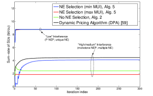
(a) Sum-rate of the SUs versus inner iterations

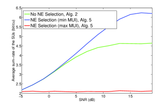
(b) Average sum-rate of the SUs versus the SNR

Figure 3: Comparison of distributed algorithms solving $\mathcal{G}_{\texttt{{siso}}}$.

Example #2 (Comparison with gradient-response algorithms for monotone VIs). In Fig. 4 we compare some algorithms solving the game $\mathcal{G}_{\texttt{{siso}}}$ under the monotonicity assumption ($\mathcal{G}_{\texttt{{siso}}}$ is a monotone NEP); the setup is the same of Fig. 3. More specifically, we plot the SUs rates versus the iteration index achieved by Algorithm 2 and the Iterative Tikhonov Algorithm recently proposed in [35] for solving monotone VIs. In the latter algorithm we chose the variable step-size sequences $\gamma_{n}=n^{-0.4}$ and $\delta_{n}=n^{-0.49}$ so that (sufficient) conditions for the convergence given in [34, Prop. 15.1] are satisfied (we use the same notation as in [35]; see therein for the details). The figure clearly shows that our best-response-based scheme converges in a very few iterations, whereas the gradient-response algorithm needs much more iterations (two orders of magnitude more) to reach comparable performance. The same convergence properties as in Fig. 4 has been experienced for all the channel realizations we simulated.

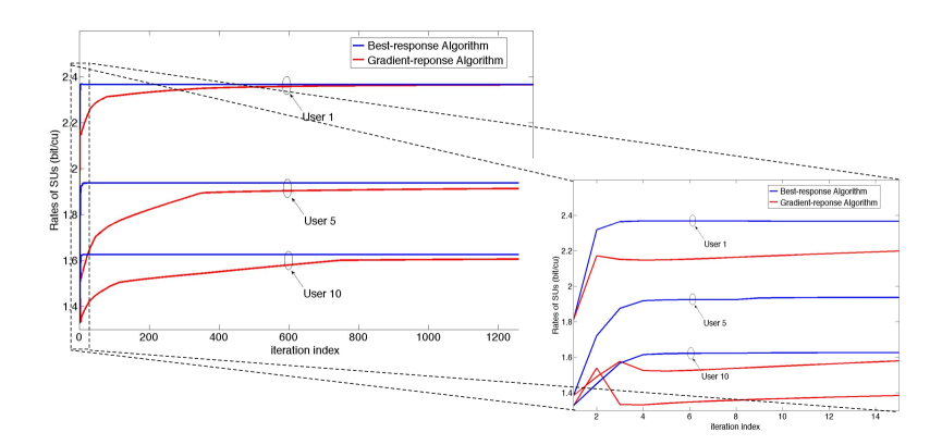
Figure 4: Typical behavior of gradient-response versus best-response algorithms solving the monotone NEP $\mathcal{G}_{\texttt{{siso}}}$: rate of three out 25 users versus the iterations achievable by the gradient-response algorithm [35] (red-line curves) and the simultaneous best-response algorithm described in Algorithm 1 (blue-line curves).

Example #3 (NE selection vs. stationary solutions: the MIMO case). We compare here some of the proposed algorithms in the MIMO setting. We consider the same scenario as in Fig. 3(a), with the only difference that now all the transceivers are equipped with three antennas and there are $I=5$ active SUs. The channels are MIMO frequency-selective (the order of the channels is $L=10$ and the number of subcarriers is $N=128$) and are generated in order to guarantee that the matrix $\boldsymbol{{\Upsilon}}_{\mathbf{F}^{\mathbb{C}}}$ in (78) is positive semidefinite, resulting thus in a monotone NEP $\mathcal{G}^{\texttt{{mimo}}}$. Soft average power shaping interference constraints are imposed to each SU along the direction of the primary transmitters; all the interference threshold are assumed to be equal and set to $I_{pi}^{\mathop{\mathrm{a}ve}}=10^{-3}$. The best-response of each user cannot be computed in closed form (unless the proximal regularization is not included in the objective function), but can be efficiently computed using any nonlinear programming solvers (each player’s optimization problem is strongly convex). In Fig. 5 we plot the sum-rate versus the inner iteration index achieved by the Jacobi version of Algorithm 2 (green-line curve), Algorithm 4.3 based on the merit function $\phi(\mathbf{Q})$ defined in (81) (blue line curve); and iii) the Gauss-Seidel based algorithm proposed in [57] to compute stationary solutions of the sum-rate problem (we adapted the algorithm in [57] including the interference constraints in the feasible set of the optimization problem). Fig. 5 shows the trade-off between performance and signaling that is achievable by the three algorithms: Algorithm 7 implementing a NE selection leads to better sum-rates than Algorithm 2 at the cost of almost the same signaling among the SUs of classical MIMO IWFAs (a constant price depending on the cross-channel matrices needs to be computing by each SU before running the algorithms); higher sum-rates can be achieved using algorithm in [57] but at the cost of more signaling among the SUs (note that in the MIMO case, the scheme [57] requires the SUs to exchange matrix informations at each iteration).

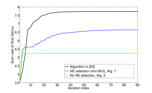
Figure 5: Comparison of distributed algorithms solving $\mathcal{G}_{\texttt{{mimo}}}$: Sum-rate of the SUs versus inner iterations.

8 Conclusions

In this paper, we have proposed a novel method based on VIs suitable to study and solve general real or complex player-convex NEPs, having (possibly) multiple solutions. The proposed framework has many desirable new features, such as: i) it can be applied to real and complex NEPs having no specific structure and for which the best-response mapping is not available in closed form or unique; ii) the algorithms proposed for computing a NE converge under mild conditions that do not imply the uniqueness of the equilibrium; and iii) in the presence of multiple equilibria, one can control the quality of the computed solution by guaranteeing convergence to the “best” NE (according to some prescribed criterion), at the cost of some signaling among the players. These features make the proposed algorithms applicable to a variety of scenarios in different fields; the choice of one scheme with respect to the other will depend on the trade-off between signaling and performance that the users are willing to exchange/achieve. The analysis of algorithms for complex NEPs hinges on the definition of the VI problem in the complex domain; this new class of VIs along with their properties are introduced and studied for the fist time in this paper.

Finally, to have suitable case studies, we applied the proposed framework to solve some novel NEPs modeling various resource allocation problems in SISO/MIMO CR systems. The resulting distributed best-response algorithms were shown to converge even when current schemes proposed in the literature for related problems fail. Numerical results showed the superiority of our (distributed) approach with respect to plain noncooperative solutions as well as good performance with respect to centralized solutions.

Appendix

Appendix A (Partitioned) Variational Inequalities

The simplest way to see a VI is as a generalization of the minimum principle for convex optimization problems, which is recalled next. Consider a convex optimization problem (in the minimization form), whose objective function $f:\mathcal{Q}\mapsto\mathbb{R}$ is convex and continuously differentiable on the feasible set $\mathcal{Q}\subseteq\mathbb{R}^{n}$, which is a convex and closed subset of $\mathbb{R}^{n}$. A point $\mathbf{x}^{\star}\in\mathcal{Q}$ is an optimal solution of the optimization problem if and only if

$$\left(\mathbf{x}-\mathbf{x}^{\star}\right)^{T}\nabla f\left(\mathbf{x}^{\star}\right)\geq 0,\qquad\forall\mathbf{x}\in\mathcal{Q}.$$ (84)

The VI problem is a generalization of the minimum principle (84) where the gradient $\nabla f$ is substituted by a general real-valued vector function $\mathbf{F}$. More formally, we have the following. Let $\mathcal{Q}\subseteq\mathbb{R}^{n}$ be a nonempty, closed, and convex set and let $\mathbf{F}:$ $\mathcal{Q}\to$ $\mathbb{R}$ⁿ be a vector-valued real function. The VI ($\mathcal{Q},$ $\mathbb{\mathbf{F)}}$ is the problem of finding a feasible point $\mathbf{x}^{\star}\in\mathcal{Q}$ such that [31, Def. 1.1.1]

$$\left(\mathbf{x}-\mathbf{x}^{\star}\right)^{T}\mathbf{F}\left(\mathbf{x}^{\star}\right)\geq 0,\qquad\forall\mathbf{x}\in\mathcal{Q}.$$ (85)

The set of solutions to this problem is denoted by $\mathop{\mathrm{S}OL}(\mathcal{Q},\mathbf{F})$.

Several standard problems in nonlinear programming, game theory, and nonlinear analysis can be naturally formulated as a VI problem; many examples can be found in [31, Ch. 1], [33], and [34]. Below we summarize some known facts and definitions about VI.

A.1 Solution analysis

In order to present results about the existence and the structure of the solution set of a VI, we introduce some function classes.

Definition 40

A mapping $\mathbf{F}:\mathcal{Q}\mathcal{\rightarrow}\mathbb{R}^{n}$, with $\mathcal{Q}$ closed and convex, is said to be

(i)

monotone on $\mathcal{Q}$ if for all pairs $\mathbf{x}$ and $\mathbf{y}$ in $\mathcal{Q}$,

$$(\,\mathbf{x}-\mathbf{y}\,)^{T}(\,\mathbf{F}(\mathbf{x})-\mathbf{F}(\mathbf{y})\,)\,\geq 0;$$ (86)

(ii)

strictly monotone if for all pairs $\mathbf{x}\neq\mathbf{y}$ in $\mathcal{Q}$ the inequality in (86) is strict;

(iii)

strongly monotone on $\mathcal{Q}$ if there exists a constant $c_{\mathop{\mathrm{s}m}}>0$ such that for all pairs $\mathbf{x}$ and $\mathbf{y}$ in $\mathcal{Q}$,

$${\displaystyle(\,\mathbf{x}-\mathbf{y}\,)^{T}(\,\mathbf{F}(\mathbf{x})-\mathbf{F}(\mathbf{y})\,)\,\geq\,c_{\mathop{\mathrm{s}m}}\,\|\,\mathbf{x}-\mathbf{y}\,\|^{2}.}$$ (87)

The constant $c_{\mathop{\mathrm{s}m}}$ is called strong monotonicity constant.

If we assume a Cartesian product structure, i.e. $\mathbf{F}=(\mathbf{F}_{i}(\mathbf{x}))_{i=1}^{I}$ and $\mathcal{Q}=\prod_{i}\mathcal{Q}_{i}$, then $\mathbf{F}$ is said to be

(iv)

a P₀ function on $\mathcal{Q}$ if for all pairs of distinct tuples $\mathbf{x}=(\mathbf{x}_{i})_{i=1}^{I}$ and $\mathbf{y}=(\mathbf{y}_{i})_{i=1}^{I}$ in $\mathcal{Q}$, an index $i$ exists such that $\mathbf{x}_{i}\neq\mathbf{y}_{i}$ and

$$(\,\mathbf{x}_{i}-\mathbf{y}_{i}\,)^{T}\left(\,\mathbf{F}_{i}(\mathbf{x})-\mathbf{F}_{i}(\mathbf{y})\,\right)\,\geq\,0;$$ (88)

(v)

a P function on $\mathcal{Q}$ if for all pairs of distinct tuples $\mathbf{x}=(\mathbf{x}_{i})_{i=1}^{I}$ and $\mathbf{y}=(\mathbf{y}_{i})_{i=1}^{I}$ in $\mathcal{Q}$, the inequality in (88) is strict;

(vi)

a uniformly P function on $\mathcal{Q}$ if there exists a constant $c_{\mathop{\mathrm{u}P}}>0$ such that for all pairs $\mathbf{x}=(\mathbf{x}_{i})_{i=1}^{I}$ and $\mathbf{y}=(\mathbf{y}_{i})_{i=1}^{I}$ in $\mathcal{Q}$,

$${\displaystyle{\max_{1\leq\,i\,\leq Q}}\,(\,\mathbf{x}_{i}-\mathbf{\mathbf{y}}_{i}\,)^{T}(\,\mathbf{F}_{i}(\mathbf{x})-\mathbf{F}_{i}(\mathbf{y})\,)\,\geq\,c_{\mathop{\mathrm{u}P}}\,\|\,\mathbf{x}-\mathbf{y}\,\|^{2}.}$$ (89)

The constant $c_{\mathop{\mathrm{u}P}}$ is called uniformly P constant.

If a function $\mathbf{F}$ enjoys one of the properties above, we will also say that the corresponding VI $(\mathcal{Q},\mathbf{F})$ enjoys the property (i.e., if $\mathbf{F}$ is monotone, we say that the VI is monotone, etc…).

Note that in the case of affine functions, $\mathbf{F}(\mathbf{x})=\mathbf{M}\mathbf{x}+\mathbf{b}$, there is no difference between strict monotonicity and strongly monotonicity, and the uniform P property coincides with the P property. Monotonicity properties play in the VI realm the same role that convex functions play in optimization. In fact, we recall that a differentiable function $f$ is convex, strictly, strongly convex on a convex set $\mathcal{Q}$ if and only if its gradient is monotone, strictly, strongly monotone on $\mathcal{Q}$. The P properties can be viewed as an extension of the monotonicity properties tailored to the possible partitioned structure of the VI; when the partitioned VI has only one block, i.e., $I=1$, the P properties collapse to the corresponding monotonicity properties. In Fig. 6 we summarize in a pictorial way some well established relations between these various classes along with some of their consequences. Theorem 41 provides instead a formal statement of some existence and uniqueness results that will be used throughout the paper.

strongly monotone	$\Rightarrow$	strictly monotone	$\Rightarrow$	monotone	$\Rightarrow$	convex solution set
$\Downarrow$		$\Downarrow$		$\Downarrow$
uniformly P	$\Rightarrow$	P	$\Rightarrow$	P0
$\Downarrow$		$\Downarrow$
unique solution	$\Rightarrow$	at most one solution

Figure 6: Monotonicity and their consequences on VIs.

Theorem 41

Given the VI $(\mathcal{Q},\,\mathbf{F})$, suppose that $\mathcal{Q}$ is closed and convex and $\mathbf{F}$ is continuous on $\mathcal{Q}$. The following statements hold:

(a)

The VI$(\mathcal{Q},\mathbf{F})$ has a (possibly empty) closed solution set. If $\mathcal{Q}$ is bounded, the solution set is nonempty and thus compact [31, Cor. 2.2.5];

(b)

If $\mathbf{F}$ is monotone on $\mathcal{Q}$, then the VI$(\mathcal{Q},\mathbf{F})$ has a (possibly empty) convex solution set [31, Th. 2.3.5];

(c)

If $\mathbf{F}$ is strictly monotone on $\mathcal{Q}$, then the VI$(\mathcal{Q},\mathbf{F})$ has at most one solution [31, Th. 2.3.3(a)]; the same conclusion holds if the VI$(\mathcal{Q},\mathbf{F})$ is partitioned and $\mathbf{F}$ is a P function on $\mathcal{Q}$ [31, Prop. 3.5.10(a)];

(d)

If $\mathbf{F}$ is strongly monotone on $\mathcal{Q}$, then the VI$(\mathcal{Q},\mathbf{F})$ has a unique solution [31, Th. 2.3.3(b)]; the same conclusion holds if the VI$(\mathcal{Q},\mathbf{F})$ is partitioned and $\mathbf{F}$ is a uniformly P function on $\mathcal{Q}$ [31, Prop. 3.5.10(b)].

Appendix B Proof of Proposition 5

Because of space limitation, we prove only (e); the proof of (a)-(d) follows similar ideas.

Given $\mathbf{x}\triangleq(\mathbf{x}_{i})_{i=1}^{I},\mathbf{y}\triangleq(\mathbf{y}_{i})_{i=1}^{I}\in\mathcal{Q}$, with $\mathbf{x}\neq\mathbf{y}$, let define the univariate continuously differentiable function $\Phi_{i}\,:\,[0,1]\ni t\,\mapsto\mathbb{R}$ as $\Phi_{i}(t)\triangleq\left(\mathbf{x}_{i}-\mathbf{y}_{i}\right)^{T}\left(\mathbf{F}_{i}\left(t\,\mathbf{x}+(1-t)\,\mathbf{y}\right)\right).$ Then, by the mean-value theorem it follows that there exists some $\bar{t}{}_{i}\in(0,1)$ such that, denoting by $\mathbf{z}_{\bar{{t}}_{i}}=\bar{{t}}_{i}\mathbf{x}+\left(1-\bar{{t}}_{i}\right)\mathbf{y}$, we have

$$\left(\mathbf{x}_{i}-\mathbf{y}_{i}\right)^{T}\left(\mathbf{F}_{i}(\mathbf{x})-\mathbf{F}_{i}(\mathbf{y})\right)=\left.\frac{d\Phi_{i}(t)}{dt}\right|_{t=\bar{{t}}_{i}}=\left(\mathbf{x}_{i}-\mathbf{y}_{i}\right)^{T}\,\sum\limits_{j=1}^{I}\mbox{J}_{i}\mathbf{F}_{j}(\mathbf{z}_{\bar{t}_{i}})\,\left(\mathbf{x}_{j}-\mathbf{y}_{j}\right)$$

$$\geq \left(\mathbf{x}_{i}-\mathbf{y}_{i}\right)^{T}\,\mbox{J}_{i}\mathbf{F}_{i}(\mathbf{z}_{\bar{t}_{i}})\,\left(\mathbf{x}_{i}-\mathbf{y}_{i}\right)-\left|\left(\mathbf{x}_{i}-\mathbf{y}_{i}\right)^{T}\,\sum\limits_{j\neq i}\mbox{J}_{i}\mathbf{F}_{j}(\mathbf{z}_{\bar{t}_{i}})\,\left(\mathbf{x}_{j}-\mathbf{y}_{j}\right)\right|$$ (90)

$$\geq \left\|\mathbf{C}_{i}^{-T}\left(\mathbf{x}_{i}-\mathbf{y}_{i}\right)\right\|^{2}\,\alpha_{i}^{\min}\,-\left\|\mathbf{C}_{i}^{-T}\left(\mathbf{x}_{i}-\mathbf{y}_{i}\right)\right\|\sum\limits_{j\neq i}\beta_{ij}^{\max}\left\|\mathbf{C}_{j}^{-T}\left(\mathbf{x}_{j}-\mathbf{y}_{j}\right)\right\|,$$

where last inequality follows from the definition of $\alpha_{i}^{\min}$ and $\beta_{ij}^{\max}$ as given in (16), and $\mathbf{C}_{i}$’s are the set of nonsingular matrices coming from (16). Introducing $\mathbf{e}=(e_{i})_{i=1}^{I}$, with each $e_{i}\triangleq\left\|\mathbf{C}_{i}^{-1}(\mathbf{x}_{i}-\mathbf{y}_{i})\right\|$, and using the definition of $\mathbf{\boldsymbol{\Upsilon}}_{\mathbf{F}}$, (90) can be written as

$$\left(\mathbf{x}_{i}-\mathbf{y}_{i}\right)^{T}\left(\mathbf{F}_{i}(\mathbf{x})-\mathbf{F}_{i}(\mathbf{y})\right)\geq e_{i}\left(\mathbf{\boldsymbol{\Upsilon}}_{\mathbf{F}}\mathbf{e}\right)_{i}.$$

Since $\mathbf{\boldsymbol{\Upsilon}}_{\mathbf{F}}$ is a P-matrix, it follows from [43, Th. 3.3.4(b)] that $c(\mathbf{\boldsymbol{\Upsilon}}_{\mathbf{F}})\triangleq\min_{\left\|\mathbf{y}\triangleq(y_{i})_{i=1}^{I}\right\|^{2}=1}\max_{i}\,y_{i}(\mathbf{\boldsymbol{\Upsilon}}_{\mathbf{F}}\,\mathbf{y})_{i}>0$. Therefore, we have

$$\max_{i=1,\ldots,I}\left(\mathbf{x}_{i}-\mathbf{y}_{i}\right)^{T}\left(\mathbf{F}_{i}(\mathbf{x})-\mathbf{F}_{i}(\mathbf{y})\right)\geq\max_{i=1,\ldots,I}\,e_{i}(\mathbf{\boldsymbol{\Upsilon}}_{\mathbf{F}}\mathbf{e})_{i}\geq\dfrac{c(\mathbf{\boldsymbol{\Upsilon}}_{\mathbf{F}})}{\max_{i=1,\ldots,I}\lambda_{\max}(\mathbf{C}_{i}^{T}\mathbf{C}_{i})}\,{\left\|\mathbf{x}-\mathbf{y}\right\|^{2}}.$$ (91)

Finally the lower bound in (17) can be proved using [43, Ex. 5.11.19], from which one can readily obtain $c(\mathbf{\boldsymbol{\Upsilon}}_{\mathbf{F}})\geq{\displaystyle\delta(\boldsymbol{\Upsilon}_{\mathbf{F}})/(I\cdot(1+\zeta(\boldsymbol{\Upsilon}_{\mathbf{F}})/\delta(\boldsymbol{\Upsilon}_{\mathbf{F}}))^{2(I-1)})}$. This completes the proof of (e). $\square$.

Appendix C Proof of Theorem 10

It is sufficient to show that, under the assumptions of the theorem, the best-response mapping is a block-contraction (i.e., a contraction with respect to some block-maximum norm); the latter property indeed guarantees that conditions of the asynchronous convergence theorem in [45, Prop. 2.1] are satisfied by the asynchronous best-response algorithm described in Algorithm 20.

We introduce first the following norms: Given the set of nonsingular matrices $\mathbf{C}_{i}$’s coming from (16), the block-maximum norm on $\mathbb{\mathbb{R}}^{n},$ with $n=n_{1}+\ldots+n_{I},$ is defined as

$$\left\|\mathbf{x}\right\|_{\text{block}}^{\mathbf{w}}\triangleq\max_{i=1,\ldots,I}\frac{\left\|\mathbf{C}_{i}^{-1}\mathbf{x}_{i}\right\|}{c_{i}},\quad\mbox{for}\quad\mathbf{x}=(\mathbf{x}_{i})_{i=1}^{I}\in\mathbb{R}^{n},$$ (92)

where $\left\|\mathbf{\bullet}\right\|$ is the Euclidean norm on $\mathbb{R}^{n_{i}}$ and $\mathbf{c}\triangleq[c_{1},\ldots,c_{I}]^{T}>\mathbf{0}$ is any positive weight vector; the (weighted) maximum norm on $\mathbb{\mathbb{R}}^{I}$ is defined as (see, e.g., [45])

$$\left\|\mathbf{x}\right\|_{\infty,\text{vec}}^{\mathbf{c}}\triangleq\max_{i=1,\ldots,I}\frac{\left|x_{i}\right|}{c_{i}},\quad\mbox{for}\quad\mathbf{x\in\mathbb{R}}^{I};$$ (93)

and the matrix norm $\left\|\mathbf{\cdot}\right\|_{\infty,\text{mat}}^{\mathbf{c}}$ on $\mathbb{R}^{I\times I}$ induced by $\left\|\cdot\right\|_{\infty,\text{vec}}^{\mathbf{c}}$ is given by

$$\left\|\mathbf{A}\right\|_{\infty,\text{mat}}^{\mathbf{c}}\triangleq\max_{i}\frac{1}{c_{i}}\mathop{\displaystyle\sum}\limits_{j=1}^{I}\left|[\mathbf{A}]_{ij}\right|c_{j},\quad\mbox{for}\quad\mathbf{A\in\mathbb{R}}^{I\times I}.$$ (94)

Under the under the P property of $\boldsymbol{{\Upsilon}}_{\mathbf{F}}$, let us introduce the best-response mapping

$$\mathcal{B}(\mathbf{x})\triangleq(\mathcal{B}_{i}(\mathbf{x}_{-i}))_{i=1}^{I}:\mathcal{Q}\ni\mathbf{x}\mapsto\mathcal{Q},\qquad\mbox{with}\qquad\mathcal{B}_{i}(\mathbf{x}_{-i})\triangleq\mbox{argmin}_{\mathbf{x}_{i}\in\mathcal{Q}_{i}}f_{i}(\mathbf{x}_{i},\,\mathbf{x}_{-i}).$$ (95)

The contraction properties of $\mathcal{B}(\mathbf{x})$ are given in the following, where $\mathbf{\boldsymbol{\Gamma}_{\mathbf{F}}}$ is defined in (15) [note that the P property of $\boldsymbol{{\Upsilon}}_{\mathbf{F}}$, implies the strong convexity of each $f_{i}(\cdot,\mathbf{x}_{-i})$ for any $\mathbf{x}_{-i}\in\mathcal{Q}_{-i}$, and thus $\alpha_{i}^{\min}>0$ for all $i$; hence, $\boldsymbol{\Gamma}_{\mathbf{F}}$ is well-defined].

Proposition 42

Suppose that $\boldsymbol{{\Upsilon}}_{\mathbf{F}}$ in (15) is a P matrix. Then, the best-response mapping $\mathcal{B}(\mathbf{x})$ is a block-contraction, i.e., there there exists some $\mathbf{c}>\mathbf{0}$ such that

$$\left\|\mathcal{B}(\mathbf{x})-\mathcal{B}(\mathbf{y})\right\|_{\text{\emph{block}}}^{\mathbf{c}}\leq\alpha_{\mathbf{c}}\left\|\mathbf{x}-\mathbf{y}\right\|_{\text{\emph{block}}}^{\mathbf{c}}\qquad\forall\mathbf{x},\mathbf{y}\in\mathcal{Q}$$ (96)

with $\alpha_{\mathbf{c}}\triangleq\left\|\mathbf{\boldsymbol{\Gamma}_{\mathbf{F}}}\right\|_{\infty,\text{\emph{mat}}}^{\mathbf{c}}<1$.

Proof. For any two vectors $\mathbf{x},\mathbf{y}\in\mathcal{Q}$ we have by the minimum principle

$$\begin{array}[]{c}\left(\mathbf{z}_{i}-\mathcal{B}_{i}(\mathbf{x})\right)^{T}\nabla_{\mathbf{x}_{i}}f_{i}\left(\mathcal{B}_{i}(\mathbf{x}),\,\mathbf{x}_{-i}\right)\geq 0\qquad\forall\mathbf{z}_{i}\in\mathcal{Q}_{i},\quad i=1,\ldots,I,\\ \left(\mathbf{z}_{i}-\mathcal{B}_{i}(\mathbf{y})\right)^{T}\nabla_{\mathbf{x}_{i}}f_{i}\left(\mathcal{B}_{i}(\mathbf{y}),\,\mathbf{y}_{-i}\right)\geq 0\qquad\forall\mathbf{z}_{i}\in\mathcal{Q}_{i},\quad i=1,\ldots,I.\end{array}$$ (97)

Substituting $\mathbf{z}_{i}=\mathcal{B}_{i}(\mathbf{y})$ into the former inequality and $\mathbf{z}_{i}=\mathcal{B}_{i}(\mathbf{x})$ into the latter, adding the two resulting inequalities we obtain with $\hat{\mathbf{z}}{}_{i}\triangleq t_{i}(\mathcal{B}_{i}(\mathbf{y}),\mathbf{y}_{-i})+(1-t_{i})(\mathcal{B}_{i}(\mathbf{x}),\mathbf{x}_{-i})$ and some $t_{i}\in(0,1)$:

$$0 \leq \left(\mathcal{B}_{i}(\mathbf{x})-\mathcal{B}_{i}(\mathbf{y})\right)^{T}\left(\nabla_{\mathbf{x}_{i}}f_{i}\left(\mathcal{B}_{i}(\mathbf{y}),\,\mathbf{y}_{-i}\right)-\nabla_{\mathbf{x}_{i}}f_{i}\left(\mathcal{B}_{i}(\mathbf{x}),\,\mathbf{x}_{-i}\right)\right)$$ (98)

$$= \left(\mathcal{B}_{i}(\mathbf{x})-\mathcal{B}_{i}(\mathbf{y})\right)^{T}\nabla_{\mathbf{x}_{i}\mathbf{x}_{i}}^{2}f_{i}\left(\hat{\mathbf{z}}\right)\left(\mathcal{B}_{i}(\mathbf{y})-\mathcal{B}_{i}(\mathbf{x})\right)+\left(\mathcal{B}_{i}(\mathbf{x})-\mathcal{B}_{i}(\mathbf{y})\right)^{T}\sum_{j\neq i}\nabla_{\mathbf{x}_{i}\mathbf{x}_{j}}^{2}f_{i}\left(\hat{\mathbf{z}}\right)\left(\mathbf{y}_{j}-\mathbf{x}_{j}\right)$$

where the equality follows from the application of the main-value theorem to the univariate, differentiable, scalar function

$$[0,\,1]\ni t_{i}\mapsto\left(\mathcal{B}_{i}(\mathbf{x})-\mathcal{B}_{i}(\mathbf{y})\right)^{T}\nabla_{\mathbf{x}_{i}}f_{i}\left(t_{i}(\mathcal{B}_{i}(\mathbf{y}),\mathbf{y}_{-i})+(1-t_{i})(\mathcal{B}_{i}(\mathbf{x}),\mathbf{x}_{-i})\right).$$ (99)

Using the definition of $\alpha_{i}^{\min}$ and $\beta_{ij}^{\max}$ as given in (16), we deduce from the inequality in (98)

$$\left\|\mathcal{B}_{i}(\mathbf{x})-\mathcal{B}_{i}(\mathbf{y})\right\|_{i}\alpha_{i}^{\min}\leq\sum_{j\neq i}\beta_{ij}^{\max}\left\|\mathbf{x}_{j}-\mathbf{y}_{j}\right\|_{j},\qquad i=1,\ldots,I,$$ (100)

(the inequality in (98) is trivially satisfied if $\left\|\mathcal{B}_{i}(\mathbf{x})-\mathcal{B}_{i}(\mathbf{y})\right\|_{i}=0$). Introducing the vectors $\mathbf{e}_{\mathcal{B}}\triangleq(e_{\mathcal{B}_{i}})_{i=1}^{I}$ and $\mathbf{e}\triangleq(e_{i})_{i=1}^{I}$ with $e_{\mathcal{B}_{i}}\triangleq\left\|\mathcal{B}_{i}(\mathbf{x})-\mathcal{B}_{i}(\mathbf{y})\right\|_{i}$ and $e_{i}=\left\|\mathbf{x}_{i}-\mathbf{y}_{i}\right\|_{i}$, using the definition of $\boldsymbol{\Gamma}_{\mathbf{F}}$ in (15), and the fact that $\alpha_{i}^{\min}>0$ for all $i$, (100) can be written in vectorial form as

$$\mathbf{e}_{\mathcal{B}}\leq\boldsymbol{{\Gamma}}_{\mathbf{F}}\,\mathbf{e},\qquad\forall\mathbf{x},\mathbf{y\in\mathcal{Q}}.$$ (101)

It follows from (101) that, for any given $\mathbf{c}>0$, we have

$$\left\|\mathcal{B}(\mathbf{x})-\mathcal{B}(\mathbf{y})\right\|_{\text{{block}}}^{\mathbf{c}}=\left\|\mathbf{e}_{\mathcal{B}}\right\|_{\infty,\text{{vec}}}^{\mathbf{c}}\leq\left\|\boldsymbol{{\Gamma}}_{\mathbf{F}}\right\|_{\infty,\text{{mat}}}^{\mathbf{c}}\left\|\mathbf{e}\right\|_{\infty,\text{{vec}}}^{\mathbf{c}}=\left\|\boldsymbol{{\Gamma}}_{\mathbf{F}}\right\|_{\infty,\text{{mat}}}^{\mathbf{c}}\left\|\mathbf{x}-\mathbf{y}\right\|_{\text{{block}}}^{\mathbf{c}}$$ (102)

which proves the inequality in (96). To complete the proof we need to show that $\left\|\boldsymbol{{\Gamma}}_{\mathbf{F}}\right\|_{\infty,\mbox{mat}}^{\mathbf{c}}<1$ for some $\mathbf{c}>0$. Invoking [43, Lemma 13.14] and [45, Cor. 6.1], we obtain the desired result:

$$\boldsymbol{{\Upsilon}}_{\mathbf{F}}\mbox{ is a P-matrix}\qquad\Leftrightarrow\qquad\exists\,\bar{{\mathbf{c}}}>0\quad\mbox{such that }\left\|\mathbf{\boldsymbol{{\Gamma}}_{\mathbf{F}}}\right\|_{\infty,\text{mat}}^{\bar{{\mathbf{c}}}}<1.$$ (103)

 

Appendix D Proof of Proposition 15

Since $\mathcal{G}$ is a monotone NEP, the VI associated with the NEP $\mathcal{G}_{\tau,\mathbf{y}}-$the VI$(\mathcal{Q},\mathbf{F}+\tau(\mathbf{I}-\mathbf{y}))$ with $\mathbf{F}=(\nabla_{\mathbf{x}_{i}}f_{i})_{i=1}^{I}-$is strongly monotone on $\mathcal{Q}$; it follows by Theorem 3(d) that $\mathcal{G}_{\tau,\mathbf{y}}$ has a unique NE for any given $\tau>0$ and $\mathbf{y}\in\mathbb{R}^{n}$. Let us denote such a unique NE by $\mathbf{S}_{\tau}(\mathbf{y})\triangleq\mathop{\mathrm{S}OL}(\mathcal{Q},\mathbf{F}+\tau(\mathbf{I}-\mathbf{y}))$.

Necessity: Let $\mathbf{x}^{\star}\in\mathcal{Q}$ be a NE of the monotone NEP $\mathcal{G}$. By Proposition 2, $\mathbf{x}^{\star}\in\mathop{\mathrm{S}OL}(\mathcal{Q},\mathbf{F})$; then the following hold: $\forall\mathbf{x}\in\mathcal{Q}$,

$$\left(\mathbf{x}-\mathbf{x}^{\star}\right)^{T}\mathbf{F}(\mathbf{x}^{\star}) \geq 0\,\,\,\Leftrightarrow\,\,\,\left(\mathbf{x}-\mathbf{x}^{\star}\right)^{T}\left(\mathbf{F}(\mathbf{x}^{\star})+\tau(\mathbf{x}^{\star}-\mathbf{x}^{\star})\right)\geq 0\,\,\,\Rightarrow\,\,\,\mathbf{x}^{\star}=\mathop{\mathrm{S}OL}\left(\mathcal{Q},\mathbf{F}+\tau(\mathbf{I}-\mathbf{x}^{\star})\right)=\mathbf{S}_{\tau}(\mathbf{x}^{\star}),$$

implying that $\mathbf{x}^{\star}$ is the unique NE of $\mathcal{G}_{\tau,\mathbf{x}^{\star}}$.

Sufficiency: Let $\mathbf{x}^{\star}$ be a NE of $\mathcal{G}_{\tau,\mathbf{x}^{\star}}$. Then, we have $\mathbf{x}^{\star}=\mathbf{S}_{\tau}(\mathbf{x}^{\star})$, which leads to the desired result: $\forall\mathbf{x}\in\mathcal{Q}$,

$$\left(\mathbf{x}-\mathbf{S}_{\tau}(\mathbf{x}^{\star})\right)^{T}\left(\mathbf{F}\left(\mathbf{S}_{\tau}(\mathbf{x}^{\star})\right)+\tau(\mathbf{S}_{\tau}(\mathbf{x}^{\star})-\mathbf{x}^{\star})\right)\geq 0\,\,\,\Leftrightarrow\,\,\,\left(\mathbf{x}-\mathbf{x}^{\star}\right)^{T}\mathbf{F}(\mathbf{x}^{\star}) \geq 0.$$

Appendix E Proof of Theorem 21

To prove the theorem we hinge on the theory of VIs. We preliminary observe that the game $\mathcal{G}$ is equivalent to the VI$(\mathcal{Q},\mathbf{F})$, with $\mathbf{F}=(\nabla_{\mathbf{x}_{i}}f_{i})_{i=1}^{I}$ (Proposition 2); $\mathop{\mathrm{S}OL}(\mathcal{Q},\mathbf{f})$ is thus also the solution set of the VI, i.e., $\mathop{\mathrm{S}OL}(\mathcal{Q},\mathbf{F})=\mathop{\mathrm{S}OL}(\mathcal{Q},\mathbf{f})$. Moreover, still invoking Proposition 2, we have that the game $\mathcal{G}_{\tau,\varepsilon^{(n)},\mathbf{x}^{(n)}}$ in Step 2 of Algorithm 4.3 is equivalent to the VI$(\mathcal{Q},\mathbf{F}^{(n)})$, where

$$\mathbf{F}^{(n)}(\mathbf{x})\triangleq\mathbf{F}(\mathbf{x})+\varepsilon^{(n)}\nabla\phi(\mathbf{x})+\tau\,(\mathbf{x}-\mathbf{x}^{(n)}).$$ (104)

Observe that, under the assumptions of the theorem, $\mathbf{F}^{(n)}$ is strongly monotone [Definition 40(iii)], implying that the VI$(\mathcal{Q},\mathbf{F}^{(n)})$ has a unique solution [Theorem 41(c)] and thus $\mathbf{x}^{(n+1)}$ in Step 2 of Algorithm 4.3 is well defined at each iteration. Moreover, denoting by $\mathcal{S}$ the solution set of (26), assumptions of the theorem, ensure that $\mathcal{S}$ is nonempty, bounded, and convex. Let us introduce for each $n$,

$$\delta^{(n)}\,\triangleq\,\dfrac{1}{2}\,\text{{dist}}(\mathbf{x}^{(n)},\mathcal{S})\,=\dfrac{1}{2}\,\|\mathbf{x}^{(n)}-{P}_{\mathcal{S}}(\mathbf{x}^{(n)})\|^{2},$$

where $P_{\mathcal{S}}(\mathbf{y})\triangleq\text{argmin}_{\mathbf{x}\in\mathcal{S}}\|\mathbf{x}-\mathbf{y}\|$ denotes the Euclidean projection on the nonempty, closed, and convex set $\mathcal{S}$. Then, to prove the theorem it suffices to show that the sequence $\{\delta^{(n)}\}$ converges to zero. Observe first that, since $\mathbf{x}^{(n+1)}$ at Step 2 is the solution of the game $\mathcal{G}_{\tau,\varepsilon^{(n)},\mathbf{x}^{(n)}}$$-$the VI$(\mathcal{K},\mathbf{F}^{(n)})$$-$we get, for any $\mathbf{y}\in\mathcal{Q}$,

$$\left[\,\mathbf{F}(\mathbf{x}^{(n+1)})+\varepsilon^{(n)}\nabla\phi(\mathbf{x}^{(n+1)})\,\right]^{T}(\,\mathbf{y}-\mathbf{x}^{(n+1)}\,)\geq\,\tau\,(\,\mathbf{x}^{(n)}-\mathbf{x}^{(n+1)}\,)^{T}(\,\mathbf{y}-\mathbf{x}^{(n+1)}\,).$$ (105)

We can write

$$\begin{array}[]{lll}\delta^{(n+1)}-\delta^{(n)}&=&\dfrac{1}{2}\,\|\,\mathbf{x}^{(n+1)}-P_{\mathcal{S}}(\mathbf{x}^{(n+1)})\,\|^{2}-\dfrac{1}{2}\,\|\,\mathbf{x}^{(n)}-P_{\mathcal{S}}(\mathbf{x}^{(n)})\,\|^{2}\vskip 3.0pt plus 1.0pt minus 1.0pt\\ &\overset{(a)}{\leq}&\dfrac{1}{2}\,\|\mathbf{x}^{(n+1)}-P_{\mathcal{S}}(\mathbf{x}^{(n)})\|^{2}-\dfrac{1}{2}\,\|\,\mathbf{x}^{(n)}-P_{\mathcal{S}}(\mathbf{x}^{(n)})\,\|^{2}\vskip 3.0pt plus 1.0pt minus 1.0pt\\ &=&-\dfrac{1}{2}\|\mathbf{x}^{(n+1)}-\mathbf{x}^{(n)}\|^{2}+\,(\mathbf{x}^{(n)}-\mathbf{x}^{(n+1)})^{T}(P_{\mathcal{S}}(\mathbf{x}^{(n)})-\mathbf{x}^{(n+1)})\vskip 3.0pt plus 1.0pt minus 1.0pt\\ &\overset{(b)}{\leq}&-\,\dfrac{1}{2}\,\|\mathbf{x}^{(n+1)}-\mathbf{x}^{(n)}\|^{2}+{\displaystyle{\dfrac{1}{\tau}}\,\mathbf{F}(\mathbf{x}^{(n+1)})^{T}(P_{\mathcal{S}}(\mathbf{x}^{(n)})-\mathbf{x}^{(n+1)})}+\,{\dfrac{\varepsilon^{(n)}}{\tau}}\,\nabla\phi(\mathbf{x}^{(n+1)})^{T}(P_{\mathcal{S}}(\mathbf{x}^{(n)})-\mathbf{x}^{(n+1)})\,\vskip 3.0pt plus 1.0pt minus 1.0pt\\ &\overset{(c)}{\leq}&-\dfrac{1}{2}\,\|\mathbf{x}^{(n+1)}-\mathbf{x}^{(n)}\|^{2}+\,{\displaystyle{\dfrac{\varepsilon^{(n)}}{\tau}}\,\underbrace{\nabla\phi(\mathbf{x}^{(n+1)})^{T}\,(P_{\mathcal{S}}(\mathbf{x}^{(n)})-\mathbf{x}^{(n+1)})}_{V^{(n+1)}}}\end{array}$$ (111)

where: (a) follows readily from the definition of projection; (b) comes from (105) evaluated at $\mathbf{y}=P_{\mathcal{S}}(\mathbf{x}^{(n)})\in\mathcal{Q}$; and (c) can be obtained by observing that since $P_{\mathcal{S}}(\mathbf{x}^{(n)})\in\mathcal{S}\subseteq\mathop{\mathrm{S}OL}(\mathcal{Q},\mathbf{F})$ and $\mathbf{x}^{(n+1)}\in\mathcal{Q}$, we have $\mathbf{F}(P_{\mathcal{S}}(\mathbf{x}^{(n)}))^{T}\,(\mathbf{x}^{(n+1)}-P_{\mathcal{S}}(\mathbf{x}^{(n)}))\geq 0$, which yields in turn, by the monotonicity of $\mathbf{F}$ [Definition 40(i)], $\mathbf{F}(\mathbf{x}^{(n+1)})^{T}\,(P_{\mathcal{S}}(\mathbf{x}^{(n)})-\mathbf{x}^{(n+1)})\leq 0$. We now distinguish three cases.

Case 1: Eventually, $V^{(n+1)}\leq 0$.

In this case the nonnegative sequence $\{\delta^{(n)}\}$ is (eventually) non-increasing and therefore convergent. Let us denote by $n_{0}$ the index from which all $V^{(n)}$ are non positive, and let us consider $n\geq n_{0}$ without loss of generality. Since $\mathcal{S}$ is bounded, this implies that also $\{\mathbf{x}^{(n)}\}$ is bounded. Furthermore, it follows from (111) that $\{\delta^{(n+1)}-\delta^{(n)}\}$ converges to zero and $\delta^{(n+1)}-\delta^{(n)}\,\leq\,-({1}/{2})\,\|\mathbf{x}^{(n+1)}-\mathbf{x}^{(n)}\|^{2},$ which shows that

$$\lim_{n\to\infty}\,\|\mathbf{x}^{(n+1)}-\mathbf{x}^{(n)}\|\,=\,0.$$ (112)

Summing (111) from $n_{0}$ to $n-1$, we get

$$\delta^{(n)}-\delta^{(n_{0})}\,\leq\,\dfrac{1}{\tau}\sum_{i=n_{0}}^{n-1}\varepsilon^{(i)}V^{(i+1)}.$$

Since $\{\delta^{(n)}\}$ converges and $V^{(n)}\leq 0$ and $\sum_{n}\varepsilon^{(n)}=\infty$ in the theorem implies that ${\displaystyle{\limsup_{n\to\infty}}\,V^{(n)}=0}$. Then, there exists a subsequence $J$ such that

$${\displaystyle{\lim_{{{n\in J}\atop{n\to\infty}}}}\,V^{(n)}\,=\,0.}$$ (113)

Since $\{\mathbf{x}^{(n)}\}$ is bounded we may assume, without loss of generality, that $\lim_{{{n\in J}\atop{n\to\infty}}}\mathbf{x}^{(n)}\,=\,\widetilde{\mathbf{x}}.$ Note that, since $\mathcal{Q}$ is closed, $\widetilde{\mathbf{x}}\in\mathcal{Q}$. We show that actually $\widetilde{\mathbf{x}}\in\mathop{\mathrm{S}OL}(\mathcal{Q},\mathbf{F})$. If this is not so, there exists a point $\mathbf{y}\in\mathcal{Q}$ such that $\mathbf{F}(\widetilde{\mathbf{x}})^{T}(\mathbf{y}-\widetilde{\mathbf{x}})<0$. Since $\mathbf{x}^{(n)}$ is the solution of the VI$(\mathcal{K},\mathbf{F}^{(n)})$ in Step 2 of the algorithm, we can write,

$$\left[\,\mathbf{F}(\mathbf{x}^{(n)})+\tau\,(\,\mathbf{x}^{(n)}-\mathbf{x}^{(n-1)}\,)\,\right]^{T}(\,\mathbf{y}-\mathbf{x}^{(n)}\,)+\,\varepsilon^{(n-1)}\,\nabla\phi\left(\mathbf{x}^{(n)}\right)^{T}(\,\mathbf{y}-\mathbf{x}^{(n)}\,)\,\geq\,0.$$ (114)

By continuity, the definition of $\mathbf{y}$, the boundedness of $\{\mathbf{x}^{(n)}\}$, and (112), we have, without loss of generality (after a suitable renumeration),

$$\lim_{{{n\in J}\atop{n\to\infty}}}\mathbf{F}(\mathbf{x}^{(n)})^{T}(\mathbf{y}-\mathbf{x}^{(n)})\,<\,0,\quad\lim_{{{n\in J}\atop{n\to\infty}}}\tau(\mathbf{x}^{(n)}-\mathbf{x}^{(n-1)})^{T}(\mathbf{y}-\mathbf{x}^{(n)})\,=\,0,\quad\lim_{{{n\in J}\atop{n\to\infty}}}\varepsilon^{(n-1)}\nabla\phi(\mathbf{x}^{(n)})^{T}(\,\mathbf{y}-\mathbf{x}^{(n)}\,)\,=\,0,$$

which contradicts (114). Therefore $\widetilde{\mathbf{x}}\in\mathop{\mathrm{S}OL}(\mathcal{Q},\mathbf{F})$.

Thanks to (112) we have ${\displaystyle{\lim_{n\in J,n\to\infty}}\,\mathbf{x}^{(n-1)}=\widetilde{\mathbf{x}}}$. Therefore, by (113) and continuity, we get $\nabla\phi(\widetilde{\mathbf{x}})^{T}(P_{\mathcal{S}}(\widetilde{\mathbf{x}})-\widetilde{\mathbf{x}})=0$. But the convexity of $\phi$ implies that $\phi(P_{\mathcal{S}}(\widetilde{\mathbf{x}}))\,\geq\,\phi(\widetilde{\mathbf{x}})+\nabla\phi(\widetilde{\mathbf{x}})^{T}(P_{\mathcal{S}}(\widetilde{\mathbf{x}})-\widetilde{\mathbf{x}})\,=\,\phi(\widetilde{\mathbf{x}}),$ thus showing that $\widetilde{\mathbf{x}}\in\mathcal{S}$. Therefore we get $\lim_{{{n\in J}\atop{n\to\infty}}}\delta^{(n)}\,=\,0.$ But since the whole sequence $\{\delta^{(n)}\}$ is convergent, this implies that the entire sequence $\{\delta^{(n)}\}$ converges to 0, thus concluding the analysis of Case 1.

Case 2: The two index sets $J$ and $\bar{J}$ are both infinite, where $J\,\triangleq\,\left\{\,n\,\mid\,V^{(n)}>0\,\right\}$ and

$$\bar{J}\,\triangleq\,\left\{\,n\,\in\,J\,\mid\,-\dfrac{1}{2}\,\|\,\mathbf{x}^{(n)}-\mathbf{x}^{(n-1)}\,\|^{2}+{\displaystyle{\dfrac{\varepsilon^{(n-1)}}{\tau}}\,V^{(n)}\,>\,0\,}\right\}.$$

By (111), if $n\in\bar{J}$ it might happen that $\delta^{(n)}>\delta^{(n-1)}$, while if $n\not\in\bar{J}$ then necessarily $\delta^{(n)}\leq\delta^{(n-1)}$. Therefore, since $\bar{J}$ is infinite, to prove that $\{\delta^{(n)}\}$ goes to zero it is enough to show that the subsequence $\{\delta^{(n)}\}_{\bar{J}}$ converges to zero. To this end, first observe that for every $n\in\bar{J}$ it holds that

$$\varepsilon^{(n-1)}V^{(n)}\,>\,\dfrac{\tau}{2}\,\|\mathbf{x}^{(n)}-\mathbf{x}^{(n-1)}\|^{2}.$$ (115)

The sequence $\{\mathbf{x}^{(n)}\}_{\bar{J}}$ is bounded since the definition of $V^{(n)}$, (115) and convexity imply $\phi(P_{\mathcal{S}}(\mathbf{x}^{(n-1)}))\,\geq\,\phi(\mathbf{x}^{(n)}).$ But $\phi(P_{\mathcal{S}}(\mathbf{x}^{(n-1)}))$ is the optimal value of (26) and therefore is a number, say $\beta$, that does not depend on the iteration $n$. Therefore, since $\mathbf{x}^{(n-1)}$ belongs to $\mathcal{Q}$, we have that $\{\mathbf{x}^{(n)}\}_{\bar{J}}$ is bounded. By continuity, also $\{V^{(n)}\}_{\bar{J}}$ is bounded. Hence, since $\{\varepsilon^{(n)}\}$ converges to $0$, (115) yields

$$\lim_{{{n\in\bar{J}}\atop{n\to\infty}}}\,\|\mathbf{x}^{(n)}-\mathbf{x}^{(n-1)}\|\,=\,0.$$ (116)

Since $\{\mathbf{x}^{(n)}\}_{\bar{J}}$ is bounded, it has limit points. Let $\tilde{J}\subseteq\bar{J}$ be a subsequence such that $\lim_{{{n\in\tilde{J}}\atop{n\to\infty}}}\,=\,\widetilde{\mathbf{x}}.$ Reasoning exactly as in Case 1, (the only difference is that instead of (112) we use (116)), we may deduce that $\widetilde{\mathbf{x}}\in\mathop{\mathrm{S}OL}(\mathcal{Q},\mathbf{F})$. By continuity, $\nabla\phi(\widetilde{\mathbf{x}})^{T}(P_{\mathcal{S}}(\widetilde{\mathbf{x}})-\widetilde{\mathbf{x}})\geq 0$. Thus $\widetilde{\mathbf{x}}\in\mathcal{S}$; hence ${\lim_{{{n\in\tilde{J}}\atop{n\to\infty}}}}\delta^{(n)}=0$. Since this reasoning can be repeated for every convergent subsequence of $\{{\mathbf{x}}^{(n)}\}_{\bar{J}}$, we conclude that ${\lim_{{{n\in\bar{J}}\atop{n\to\infty}}}}\,\delta^{(n)}=0$, thus concluding the analysis of this case.

Case 3: The index set $J$ is infinite while $\bar{J}$ is finite. In this case, the sequence $\{\delta^{(n)}\}$ is non-increasing eventually. Therefore $\{\delta^{(n)}\}$ converges, implying that $\{\mathbf{x}^{(n)}\}$ is bounded, $\{\delta^{(n+1)}-\delta^{(n)}\}$ converges to zero and therefore, by (111), also (112) holds. At this point, we can proceed exactly as in Case 1 and Case 2 to prove that $\{\delta^{(n)}\}$ converges to zero, thus concluding the proof of the theorem. $\square$

Appendix F Proof of Lemma 23

To prove the lemma it is sufficient to show that the first-order Taylor expansion as given in (35) holds for the function $f$; the rest of the proof follows similar steps as those used to prove the minimum principle for (real-valued) functions of real variables and thus is omitted; see e.g., [54].

Before proving the lemma, it is useful to introduce a real-coordinate representation of real-valued functions of complex matrices and establish the connection between standard derivatives of this representation and the $\mathbb{R}$-derivatives of the original functions of complex variables.

The complex space $\mathbb{C}^{n\times m}$ of dimension $n\cdot m$ has a natural structure of a real space $\mathbb{R}^{2nm}$ of dimensions $2n\cdot m$; this comes readily, e.g., from the following isomorphic transformation:

$$\mathbb{C}^{n\times m}\ni\mathbf{Z}\Longleftrightarrow\check{\mathbf{z}}\triangleq\left[\begin{array}[]{c}\text{{vec}}\left(\text{{Re}}(\textbf{Z})\right)\\ \text{{vec}}\left(\text{{Im}}(\textbf{Z})\right)\end{array}\right]\in\mathbb{R}^{2nm}.$$ (117)

For the sake of simplicity, in the following, we will denote by $\mathcal{Z}\triangleq\mathbb{C}^{n\times m}$ the original complex space and by $\mathbf{Z}$ the elements of $\mathcal{Z}$; $\mathcal{R}\triangleq\mathbb{R}^{2nm}$ will be the $2n\cdot m$-dimensional space of real vectors in the form $\check{\mathbf{z}}$, i.e.,

$$\mathcal{R}\triangleq\left\{\check{\mathbf{z}}\in\mathbb{R}^{2nm}\,:\,\check{\mathbf{z}}\triangleq\left[\begin{array}[]{c}\check{\mathbf{z}}_{R}\\ \check{\mathbf{z}}_{I}\end{array}\right]\triangleq\left[\begin{array}[]{c}\text{{vec}}\left(\text{{Re}}(\textbf{Z})\right)\\ \text{{vec}}\left(\text{{Im}}(\textbf{Z})\right)\end{array}\right],\,\mbox{for some }\mathbf{Z}\in\mathcal{Z}\right\};$$ (118)

elements of $\mathcal{R}$ will be denoted by $\check{\mathbf{z}}$, and partitioned as in (118).

Given a real-valued function of complex matrices $f:\mathcal{Z}\rightarrow\mathbb{R}$, the representation of $f(\mathbf{Z})$ under the isomorphic transformation (117) is denoted by $\check{f}(\check{\mathbf{z}})=f(\mathbf{Z})$. Note that if $f(\mathbf{Z})$ is $\mathbb{R}$-(continuously) differentiable on $\mathcal{Z}$ then $\check{f}(\check{\mathbf{z}})$ is (continuously) differentiable on $\mathcal{R}$. Moreover, we can easily establish the connection between the Jacobian of $\check{f}(\check{\mathbf{z}})$ and the Jacobian and conjugate Jacobian of $f(\mathbf{Z})$ [cf. (32)], as shown next. By definition, for any $\check{\mathbf{z}}\in\mathcal{R}$, the Jacobian of $\check{f}(\check{\mathbf{z}})$ is

$$D_{\check{\mathbf{z}}}\check{f}(\check{\mathbf{z}})\triangleq\left(\nabla_{\check{\mathbf{z}}}\check{f}(\check{\mathbf{z}})\right)^{T}=\left[\dfrac{{\partial}\check{f}(\check{\mathbf{z}})}{{\partial}\check{\mathbf{z}}_{R}^{T}},\,\dfrac{{\partial}\check{f}(\check{\mathbf{z}})}{{\partial}\check{\mathbf{z}}_{I}^{T}}\right]\triangleq\left[D_{\check{\mathbf{z}}_{R}}\check{f}(\check{\mathbf{z}}),\,D_{\check{\mathbf{z}}_{I}}\check{f}(\check{\mathbf{z}})\right].$$ (119)

Using (30) and (32), it is not difficult to see that, for any given $\mathcal{Z}\ni\mathbf{Z}\Longleftrightarrow\check{\mathbf{z}}\in\mathcal{R}$, the following hold

$$D{}_{\mathbf{Z}}f\left(\mathbf{Z}\right) \triangleq\dfrac{{\partial}f\left(\mathbf{Z}\right)}{{\partial}\text{{vec}}\left(\mathbf{Z}\right)^{T}}=\dfrac{{1}}{2}\,\left[D_{\check{\mathbf{z}}_{R}}\check{f}(\check{\mathbf{z}})-j\cdot D_{\check{\mathbf{z}}_{I}}\check{f}(\check{\mathbf{z}})\right],$$ (120)

$$D{}_{\mathbf{Z}^{\ast}}f\left(\mathbf{Z}\right) \triangleq\dfrac{{\partial}f\left(\mathbf{Z}\right)}{{\partial}\text{{vec}}\left(\mathbf{Z}^{\ast}\right)^{T}}=\dfrac{{1}}{2}\,\left[D_{\check{\mathbf{z}}_{R}}\check{f}(\check{\mathbf{z}})+j\cdot D_{\check{\mathbf{z}}_{I}}\check{f}(\check{\mathbf{z}})\right],$$ (121)

which provides the desired relationship between $D_{\check{\mathbf{z}}}\check{f}(\check{\mathbf{z}})$ and $D{}_{\mathbf{Z}}f\left(\mathbf{Z}\right)$ and $D{}_{\mathbf{Z}^{\ast}}f\left(\mathbf{Z}\right)$.

Exploring the above equivalences, we can now readily prove Lemma 23 leveraging on standard real calculus results. Given a real-valued convex and continuously $\mathbb{R}$-differentiable function $f:\mathcal{K}\rightarrow\mathbb{R}$ on $\mathcal{K}$, the first-order Taylor expansion of $f(\mathbf{Z})=\check{f}(\check{\mathbf{z}})$ at $\mathcal{K}\ni\mathbf{Z}_{0}(\Leftrightarrow\check{\mathbf{z}}_{0})$ exists and it is given by:

$$f(\mathbf{\mathbf{Z}_{0}}+\Delta\mathbf{Z})-f(\mathbf{Z}_{0})\,= \,\check{f}(\check{\mathbf{z}}_{0}+\Delta\check{\mathbf{z}})-\check{f}(\check{\mathbf{z}}_{0})$$

$$\simeq \,D_{\check{\mathbf{z}}}\check{f}(\check{\mathbf{z}}_{0})\cdot\text{$\Delta\check{\mathbf{z}}$}$$ (122)

$$= \,2\,\text{{Re}}\left\{D{}_{\mathbf{Z}}f\left(\mathbf{Z}_{0}\right)\text{{vec}}\left(\Delta\mathbf{Z}\right)\right\}$$ (123)

$$= \,2\,\text{{Re}}\left\{\text{{tr}}\left(\left(\nabla_{\mathbf{Z}}f(\mathbf{Z}_{0})\right)^{T}\Delta\mathbf{Z}\right)\right\}$$ (124)

$$= \,\,2\,\left\langle\Delta\mathbf{Z},\,\nabla_{\mathbf{Z}^{\ast}}f(\mathbf{Z}_{0})\right\rangle,$$ (125)

where (122) follows from the first-order Taylor expansion of real-valued functions of real vectors (see, e.g., [54]); (123) follows from (120); (124) is due to $D{}_{\mathbf{Z}}f\left(\mathbf{Z}_{0}\right)=\text{{vec}}\left(\nabla_{\mathbf{Z}}f(\mathbf{Z}_{o})\right)^{T}$ and the property $\text{{vec}}\left(\mathbf{A}\right)^{T}\text{{vec}}\left(\mathbf{B}\right)=\text{{tr}}\left(\mathbf{A}^{T}\mathbf{B}\right)$ for any $\mathbf{A},\mathbf{B}\in\mathbb{C}^{n\times m}$; and in (125) we used the fact that $f$ is real and thus $\left(\nabla_{\mathbf{Z}}f(\mathbf{Z}_{o})\right)^{\ast}=\nabla_{\mathbf{Z}^{\ast}}f(\mathbf{Z}_{o})$. This completes the proof. $\square$

Appendix G Complex Matrix Derivatives in Example 24

We derive here the expressions of the (conjugate) derivatives used in the Example 24 and Example 24 revisited.

In order to obtain the expression of the augmented Hessian $\mathcal{H}_{\mathbf{Z}\mathbf{Z}^{\ast}}\tilde{{f}}(\mathbf{Z})$, we need to compute $\nabla_{\mathbf{Z}\mathbf{Z}^{\ast}}^{2}\tilde{{f}}({\mathbf{Z}})$ $\triangleq D_{\mathbf{Z}}\left(\nabla_{\mathbf{Z}^{\ast}}\tilde{{f}}({\mathbf{Z}})\right)$ and $\nabla_{\mathbf{Z^{\ast}}\mathbf{Z}^{\ast}}^{2}\tilde{{f}}({\mathbf{Z}})\triangleq D_{\mathbf{Z}^{\ast}}\left(\nabla_{\mathbf{Z}^{\ast}}\tilde{{f}}({\mathbf{Z}})\right)$. We preliminary compute $\nabla_{\mathbf{\mathbf{Z}}}{f}(\mathbf{Z})$ and $\nabla_{\mathbf{\mathbf{Z}^{\ast}}}{f}(\mathbf{Z})$.

Recalling that [52, Prop. 3.12] $d\ln\det\left(\mathbf{Z}\right)=\textrm{Tr}\left(\mathbf{Z}^{-1}d\mathbf{Z}\right)$ for all $\mathbf{Z}$ such that $\det\mathbf{Z}\neq 0$, with $d\ln\det\left(\mathbf{Z}\right)$ being the (complex) differential of $\ln\det\left(\mathbf{Z}\right)$, we have (up to a constant positive factor)

$$df(\mathbf{Z}) = \textrm{Tr}\left(\left(\mathbf{R}_{n}+\mathbf{HZH}^{H}\right)^{-1}\mathbf{H}d\mathbf{Z}\mathbf{H}^{H}\right)=\textrm{vec}^{T}\left(\left(\mathbf{H}^{H}\left(\mathbf{R}_{n}+\mathbf{HZH}^{H}\right)^{-1}\mathbf{H}\right)^{T}\right)\text{{vec}}(d\mathbf{Z})\vspace{-0.2cm}$$ (126)

which, using the identification rule as given in [52, Table 3.3], leads to the following Jacobian matrices of $f$:

$$D_{\mathbf{Z}}f(\mathbf{Z}) = \textrm{vec}^{T}\left(\left(\mathbf{H}^{H}\left(\mathbf{R}_{n}+\mathbf{HZH}^{H}\right)^{-1}\mathbf{H}\right)^{T}\right)\quad\mbox{and}\quad D_{\mathbf{Z^{\ast}}}f(\mathbf{Z})=\mathbf{0},$$ (127)

and thus [cf. (32)]

$$\nabla_{\mathbf{Z}}f(\mathbf{Z})=\left(\mathbf{H}^{H}\left(\mathbf{R}_{n}+\mathbf{HZH}^{H}\right)^{-1}\mathbf{H}\right)^{T}\quad\mbox{and}\quad\nabla_{\mathbf{Z^{\ast}}}f(\mathbf{Z})=\mathbf{0}.$$ (128)

It follows from (128) that

$$\nabla_{\mathbf{Z^{\ast}}}\tilde{{f}}({\mathbf{Z}})=\nabla_{\mathbf{\mathbf{Z}^{\ast}}}{f}(\mathbf{Z})+\nabla_{\mathbf{\mathbf{Z}^{\ast}}}{f}(\mathbf{Z})^{\ast}=\left(\nabla_{\mathbf{\mathbf{Z}}}{f}(\mathbf{Z})\right)^{\ast}=\mathbf{H}^{H}\left(\mathbf{R}_{n}+\mathbf{H}\mathbf{Z}^{H}\mathbf{H}^{H}\right)^{-1}\mathbf{H}.$$ (129)

Given (129), we can now compute $\nabla_{\mathbf{Z}\mathbf{Z}^{\ast}}^{2}\tilde{{f}}({\mathbf{Z}})$ and $\nabla_{\mathbf{Z^{\ast}}\mathbf{Z}^{\ast}}^{2}\tilde{{f}}({\mathbf{Z}})$. The differential of $\nabla_{\mathbf{Z^{\ast}}}\tilde{{f}}(\mathbf{Z})$ is:

$$\text{{vec}}\left[d\left(\nabla_{\mathbf{Z^{\ast}}}\tilde{{f}}(\mathbf{Z}^{\ast})\right)\right] = \textrm{vec}\left[\mathbf{H}^{H}d\left(\mathbf{R}_{n}+\mathbf{H}\mathbf{Z}^{H}\mathbf{H}^{H}\right)^{-1}\mathbf{H}\right]$$ (130)

$$= -\underset{\mathbf{G}(\mathbf{Z})\triangleq\mathbf{H}^{H}\left(\mathbf{R}_{n}+\mathbf{H}\mathbf{Z}^{H}\mathbf{H}^{H}\right)^{-1}\mathbf{H}}{\underbrace{\textrm{vec}\left[\mathbf{G}(\mathbf{Z})(d\mathbf{Z})^{H}\mathbf{G}(\mathbf{Z})\right]}}$$ (131)

$$= -\left[\mathbf{G}(\mathbf{Z})^{T}\otimes\mathbf{G}(\mathbf{Z})\right]\textrm{vec}\left[(d\mathbf{Z}^{\ast})^{T}\right]$$ (132)

$$= -\left[\mathbf{G}(\mathbf{Z})^{T}\otimes\mathbf{G}(\mathbf{Z})\right]\mathbf{K}_{n^{2}n^{2}}\textrm{vec}\left[(d\mathbf{Z}^{\ast})\right]$$ (133)

where in (131) we used the rule $d\mathbf{Z}^{-1}=-\mathbf{Z}^{-1}(d\mathbf{Z})\mathbf{Z}^{-1}$ [52, Prop. 3.8]; (132) follows from the property $\text{{vec}}(\mathbf{A}\mathbf{B}\mathbf{C})=(\mathbf{C}^{T}\otimes\mathbf{A})\,\text{{vec}}(\mathbf{B})$ [52, Lemma 2.11]; and in the last equality we introduced the commutation matrix $\mathbf{K}_{n^{2}n^{2}}$, which is the $n^{2}\times n^{2}$ permutation matrix such that $\text{{vec}}(\mathbf{A}^{T})=\mathbf{K}_{n^{2}n^{2}}\text{{vec}}(\mathbf{A})$ [52, Def. 1.8].

It follows from (133) and the identification rule [52, Table 3.3] that

$$\nabla_{\mathbf{Z}^{*}\mathbf{Z}^{\ast}}^{2}\widetilde{f}(\mathbf{Z}) = \nabla_{\mathbf{Z}\mathbf{Z}^{*}}^{2}\widetilde{f}(\mathbf{Z})-\left[\mathbf{G}(\mathbf{Z})^{T}\otimes\mathbf{G}(\mathbf{Z})\right]\mathbf{K}_{n^{2}n^{2}}\quad\mbox{and}\quad\nabla_{\mathbf{Z}\mathbf{Z}^{*}}^{2}\widetilde{f}(\mathbf{Z})=\mathbf{0},$$ (134)

which leads to the expression of the augmented Hessian $\mathcal{H}_{\mathbf{Z}\mathbf{Z}^{\ast}}\tilde{{f}}(\mathbf{Z})$ as given in (47).

Appendix H Proof of Propositions 27 and 28

It is sufficient to prove only Proposition 28; Proposition 27 is just a special case. To do that, we need the following intermediate result.

H.1 Mean-value theorem for functions of complex variables

We provide here a version of the mean-value theorem that is suitable for real-valued functions of complex matrices. We focus directly on the specific function that we need to prove Proposition 28.

Given a continuously $\mathbb{R}$-differentiable matrix function $\mathbf{F}^{\mathbb{C}}:\mathcal{K}\rightarrow\mathbb{C}^{n\times m}$ on the convex and closed set $\mathcal{K}\subseteq\mathbb{C}^{n\times m}$ and a point $\Delta\mathbf{Y}\in\mathbb{C}^{n\times m}$, let us consider the real-valued function of complex matrix variables

$$g(\mathbf{Z})\triangleq\left\langle\Delta\mathbf{Y},\,\mathbf{\mathbf{F}^{\mathbb{C}}}(\mathbf{Z})\right\rangle.$$ (135)

For every two points $\mathbf{Z}_{1},\mathbf{Z}_{2}\in\mathcal{K}$, with $\Delta\mathbf{Z}\triangleq\mathbf{Z}_{2}-\mathbf{Z}_{1}$, let $h(t):[0,1]\rightarrow\mathbb{R}$ be the real-valued scalar function, defined as $[0,1]\ni t\mapsto h(t)\triangleq\left\langle\Delta\mathbf{Y},\,\mathbf{\mathbf{F}^{\mathbb{C}}}\left(\mathbf{Z}(t)\right)\right\rangle,$ with $\mathbf{Z}(t)\triangleq\mathbf{Z}_{1}+t\,\Delta\mathbf{Z}$. For some $\bar{{t}}\in(0,1)$, we have

$$g(\mathbf{Z}_{2})-g(\mathbf{Z}_{1}) =h(1)-h(0)=h^{{}^{\prime}}(\bar{{t}})$$ (136)

where $h^{{}^{\prime}}({t})$ is the first order derivative of $h(t)$ [note that $h$ is continuously differentiable on $(0,1)$], and the last equality in (136) follows from the mean-value theorem applied to the function $h(t)$. To compute $h^{{}^{\prime}}(t)$ we use the chain rule for complex matrix derivatives [52] as shown next. Rewriting $h(t)$ as

$$h(t)=\dfrac{{1}}{2}\,\text{{tr}}\left(\Delta\textbf{Y}^{H}\,\mathbf{\mathbf{F}^{\mathbb{C}}}\left(\mathbf{Z}(t)\right)\right)+\dfrac{{1}}{2}\,\text{{tr}}\left(\Delta\textbf{Y}^{T}\,\mathbf{\mathbf{F}^{\mathbb{C}}}\left(\mathbf{Z}(t)\right)^{\ast}\right)\vspace{-0.2cm}$$ (137)

and using

$$\begin{array}[]{ll}D{}_{\mathbf{Z}}\,\text{{tr}}\left(\Delta\textbf{Y}^{H}\,\mathbf{\mathbf{F}^{\mathbb{C}}}\left(\mathbf{Z}\right)\right)=\text{{vec}}\left(\Delta\textbf{Y}^{\ast}\right)^{T}D{}_{\mathbf{Z}}\mathbf{\mathbf{F}^{\mathbb{C}}}\left(\mathbf{Z}\right)&D{}_{\mathbf{Z^{\ast}}}\,\text{{tr}}\left(\Delta\textbf{Y}^{H}\,\mathbf{\mathbf{F}^{\mathbb{C}}}\left(\mathbf{Z}\right)\right)=\text{{vec}}\left(\Delta\textbf{Y}^{\ast}\right)^{T}D{}_{\mathbf{Z}^{\ast}}\mathbf{F}^{\mathbb{C}}\left(\mathbf{Z}\right)\vskip 12.0pt plus 4.0pt minus 4.0pt\\ D{}_{\mathbf{Z}}\,\text{{tr}}\left(\Delta\textbf{Y}^{T}\,\mathbf{\mathbf{F}^{\mathbb{C}}}\left(\mathbf{Z}\right)^{\ast}\right)=\left(D{}_{\mathbf{Z^{\ast}}}\,\text{{tr}}\left(\Delta\textbf{Y}^{H}\,\mathbf{\mathbf{F}^{\mathbb{C}}}\left(\mathbf{Z}\right)\right)\right)^{\ast}&D{}_{\mathbf{Z}^{\ast}}\,\text{{tr}}\left(\Delta\textbf{Y}^{T}\,\mathbf{\mathbf{F}^{\mathbb{C}}}\left(\mathbf{Z}\right)^{\ast}\right)=\left(D{}_{\mathbf{Z}}\,\text{{tr}}\left(\Delta\textbf{Y}^{H}\,\mathbf{\mathbf{F}^{\mathbb{C}}}\left(\mathbf{Z}\right)\right)\right)^{\ast}\end{array}$$

we have

$$h^{{}^{\prime}}(t) =D{}_{\mathbf{Z}(t)}h(t)\,D{}_{t}\mathbf{Z}(t)+D{}_{\mathbf{Z}(t)^{\ast}}h(t)\,D{}_{t}\mathbf{Z}(t)^{\ast}\vskip 6.0pt plus 2.0pt minus 2.0pt$$ (138)

$$=\dfrac{{1}}{2}\,\text{{vec}}\left(\Delta\textbf{Y}^{\ast}\right)^{T}D{}_{\mathbf{Z}}\mathbf{F}^{\mathbb{C}}\left(\mathbf{Z}(t)\right)\text{{vec}}\left(\Delta\mathbf{Z}\right)+\dfrac{{1}}{2}\,\text{{vec}}\left(\Delta\textbf{Y}\right)^{T}D{}_{\mathbf{Z}}\mathbf{\mathbf{F}^{\mathbb{C}}}\left(\mathbf{Z}(t)\right)^{\ast}\text{{vec}}\left(\Delta\mathbf{Z}\right)$$

$$\quad+\dfrac{{1}}{2}\,\text{{vec}}\left(\Delta\textbf{Y}^{\ast}\right)^{T}D{}_{\mathbf{Z}^{\ast}}\mathbf{\mathbf{F}^{\mathbb{C}}}\left(\mathbf{Z}(t)\right)\text{{vec}}\left(\Delta\mathbf{Z}^{\ast}\right)+\dfrac{{1}}{2}\,\text{{vec}}\left(\Delta\textbf{Y}\right)^{T}D{}_{\mathbf{Z^{\ast}}}\mathbf{\mathbf{F}^{\mathbb{C}}}\left(\mathbf{Z}(t)\right)^{\ast}\text{{vec}}\left(\Delta\mathbf{Z}^{\ast}\right)$$

$$=\dfrac{{1}}{2}\,\text{{vec}}\left(\left[\Delta\textbf{Y},\,\Delta\textbf{Y}^{\ast}\right]\right)^{H}\left[\begin{array}[]{ll}D_{\mathbf{Z}}\mathbf{F}^{\mathbb{C}}(\mathbf{Z}(t))&D_{\mathbf{Z}^{\ast}}\mathbf{F}^{\mathbb{C}}(\mathbf{Z}(t))\\ D_{\mathbf{Z}}\mathbf{F}^{\mathbb{C}}(\mathbf{Z}(t))^{\ast}&D_{\mathbf{Z}^{\ast}}\mathbf{F}^{\mathbb{C}}(\mathbf{Z}(t))^{\ast}\end{array}\right]\text{{vec}}\left(\left[\Delta\textbf{Z},\,\Delta\textbf{Z}^{\ast}\right]\right),$$ (141)

where in (138) we used the chain rule [52, Th. 3.1]. Using (141) and the augmented Jacobian matrix $\mathbf{JF}^{\mathbb{C}}(\mathbf{Z})$ introduced in (39), we can rewrite (136) in a compact form as

$$g(\mathbf{Z}_{2})-g(\mathbf{Z}_{1})=\,\text{{vec}}\left(\left[\Delta\textbf{Y},\,\Delta\textbf{Y}^{\ast}\right]\right)^{H}\mathbf{JF}^{\mathbb{C}}(\mathbf{Z}(\bar{{t}}))\,\text{{vec}}\left(\left[\Delta\textbf{Z},\,\Delta\textbf{Z}^{\ast}\right]\right).$$ (142)

which is the desired result.

H.2 Proof of Proposition 28

We prove only (a)-(c); the proof of (d)-(e) follows similar steps.

Sufficiency part. For (a)-(c), it is enough to prove only (c). Given two points $\mathbf{Z}_{1},\mathbf{Z}_{2}\in\mathcal{K}$, let us define $\Delta\textbf{Z}\triangleq\mathbf{Z}_{2}-\mathbf{Z}_{1}$; we have, for some $\bar{{t}}\in(0,1)$,

$$\left\langle\mathbf{Z}_{2}-\mathbf{Z}_{1},\,\mathbf{\mathbf{F}^{\mathbb{C}}}\left(\mathbf{Z}_{2}\right)-\mathbf{\mathbf{F}^{\mathbb{C}}}\left(\mathbf{Z}_{1}\right)\right\rangle =\text{{vec}}\left(\left[\Delta\textbf{Z},\,\Delta\textbf{Z}^{\ast}\right]\right)^{H}\mathbf{JF}^{\mathbb{C}}(\mathbf{Z}(\bar{{t}}))\,\text{{vec}}\left(\left[\Delta\textbf{Z},\,\Delta\textbf{Z}^{\ast}\right]\right),$$ (143)

where the equality follows from (142). Since $\mathbf{Z}_{1},\mathbf{Z}_{2}\in\mathcal{K}$, we have that $\Delta\mathbf{Z}\in S_{\mathcal{K}}$; moreover $\mathbf{Z}(\bar{{t}})\in\mathcal{K}$ (due to the convexity of $\mathcal{K}$). It follows from (143) that if there exists a constant $c_{\text{{sm}}}$ such that $\text{{vec}}\left([\mathbf{Y},\mathbf{Y}^{\ast}]\right)^{H}\mathbf{JF}^{\mathbb{C}}(\mathbf{Z})$ $\text{\text{{vec}}}\left([\mathbf{Y},\mathbf{Y}^{\ast}]\right)\geq$$\,(c_{\text{{sm}}}/2)\,\left\|\mathbf{Y}\right\|_{F}^{2}$ for all $\mathbf{Y}\in\mathcal{S}_{\mathcal{K}}$ and $\mathbf{Z}\in\mathcal{K}$, then $\mathbf{\mathbf{F}^{\mathbb{C}}}\left(\mathbf{Z}\right)$ is strongly monotone on $\mathcal{K}$.

Necessity part. Let us focus on the strongly monotonicity property only; monotonicity is obtained in a similar way. Suppose that $\mathbf{\mathbf{F}^{\mathbb{C}}}\left(\mathbf{Z}\right)$ is strongly monotone on $\mathcal{K}$ with constant $c_{\text{{sm}}}>0$. Let us show first that $\text{{vec}}\left([\mathbf{Y},\mathbf{Y}^{\ast}]\right)^{H}\mathbf{JF}^{\mathbb{C}}(\mathbf{Z})\text{{vec}}\left([\mathbf{Y},\mathbf{Y}^{\ast}]\right)\geq(c_{\text{{sm}}}/2)\,\left\|\mathbf{Y}\right\|_{F}^{2}$ for all $\mathbf{Y}\in S_{\mathcal{K}}$ and $\mathbf{Z}\in\text{{ri}}(\mathcal{K})$, where $\text{{ri}}(\mathcal{K})$ denotes the relative interior of $\mathcal{K}$ (see [54, Ch. 1.4] for the definition of $\text{{ri}}(\mathcal{K})$ and its main properties). Then, we have

$$\text{{vec}}\left([\mathbf{Y},\mathbf{Y}^{\ast}]\right)^{H}\mathbf{JF}^{\mathbb{C}}(\mathbf{Z})\text{{vec}}\left([\mathbf{Y},\mathbf{Y}^{\ast}]\right) =\dfrac{{1}}{2}\,\text{{vec}}\left([\mathbf{Y},\mathbf{Y}^{\ast}]\right)^{H}\lim_{t\downarrow 0}\dfrac{{1}}{t}\left[\begin{array}[]{c}\text{{vec}}\left(\mathbf{F}^{\mathbb{C}}(\mathbf{Z}+t\mathbf{Y})-\mathbf{F}^{\mathbb{C}}(\mathbf{Z})\right)\\ \text{{vec}}\left(\mathbf{F}^{\mathbb{C}}(\mathbf{Z}+t\mathbf{Y})-\mathbf{F}^{\mathbb{C}}(\mathbf{Z})\right)^{\ast}\end{array}\right]$$ (146)

$$=\dfrac{{1}}{2}\,\lim_{t\downarrow 0}\dfrac{{1}}{t^{2}}\,\left\langle t\mathbf{Y},\mathbf{F}^{\mathbb{C}}(\mathbf{Z}+t\mathbf{Y})-\mathbf{F}^{\mathbb{C}}(\mathbf{Z})\right\rangle$$ (147)

$$\geq\dfrac{c_{\text{{sm}}}}{2}\,\lim_{t\downarrow 0}\dfrac{{1}}{t^{2}}\,\left\|t\mathbf{Y}\right\|_{F}^{2}=\dfrac{c_{\text{{sm}}}}{2}\,\left\|\mathbf{Y}\right\|_{F}^{2},\quad\forall\mathbf{Y}\in S_{\mathcal{K}}\,\mbox{and}\,\mathbf{Z}\in\text{{ri}}(\mathcal{K}),$$ (148)

where the equality in (146) follows from the ($\mathbb{R}$-)differentiability of $\mathbf{\mathbf{F}^{\mathbb{C}}}\left(\mathbf{Z}\right)$ on $\mathcal{K}$ [(146) can be proved using the same approach as in the proof of Lemma 23 but applied to $\text{{vec}}\left(\mathbf{F}^{\mathbb{C}}(\mathbf{Z})\right)$]; in (147) we used the definition of inner product (36); and in (148) we used i) the fact that for sufficiently small $t>0$, $\mathbf{Z}+t\mathbf{Y}\in\mathcal{K}$ [since $\mathbf{Z}\in\text{{ri}}(\mathcal{K})$], and ii) the strongly monotonicity of $\mathbf{F}^{\mathbb{C}}(\mathbf{Z})$ on $\mathcal{K}$.

Next, let $\mathbf{Z}\in\mathcal{K}$ but $\mathbf{Z}\notin\text{{ri}}(\mathcal{K})$; by [54, Proposition 1.4.1(a)] there exists a sequence $\{\mathbf{Z}_{k}\}\subset\text{{ri}}(\mathcal{K})$ such that $\mathbf{Z}_{k}\rightarrow\mathbf{Z}$. By (148) evaluated in each $\mathbf{Z}_{k}\in\text{{ri}}(\mathcal{K})$ and the continuity of $\mathbf{JF}^{\mathbb{C}}(\mathbf{Z})$, it is follows that

$$\text{{vec}}\left([\mathbf{Y},\mathbf{Y}^{\ast}]\right)^{H}\mathbf{JF}^{\mathbb{C}}(\mathbf{Z})\text{{vec}}\left([\mathbf{Y},\mathbf{Y}^{\ast}]\right)=\lim_{k\rightarrow\infty}\text{{vec}}\left([\mathbf{Y},\mathbf{Y}^{\ast}]\right)^{H}\mathbf{JF}^{\mathbb{C}}(\mathbf{Z}_{k})\text{{vec}}\left([\mathbf{Y},\mathbf{Y}^{\ast}]\right)\geq\dfrac{c_{\text{{sm}}}}{2}\,\left\|\mathbf{Y}\right\|_{F}^{2},$$

for all $\mathbf{Y}\in S_{\mathcal{K}}.$ This completes the proof of the necessity part.

Note that Proposition 28 reduces to Proposition 27 if the set $\mathcal{K}$ has nonempy interior. Indeed, when this happens, $\text{{Aff}}(\mathcal{K})=\mathbb{C}^{n\times m}$ and thus $S_{\mathcal{K}}=\mathbb{C}^{n\times m}$.

Appendix I Proof of Proposition 36

Statement (a) follows from Proposition 29; for (b) and (c), we prove only (b).

According to Proposition 27(a), we need to show that, under the assumption that $\boldsymbol{{\Upsilon}}_{\mathbf{F}^{\mathbb{C}}}^{\text{{{mimo}}}}$ in (78) is positive semidefinite, the augmented Jacobian matrix $\mathbf{JF}^{\mathbb{C}}(\mathbf{Q})$ associated to $\mathbf{F}^{\mathbb{C}}(\mathbf{Q})$ in (77) is augmented positive semidefinite on $\mathcal{P}^{\texttt{{mimo}}}$. Given (77), $D_{\mathbf{Q}^{\star}}\mathbf{F}^{\mathbb{C}}(\mathbf{Q})=\mathbf{0}$, implying that $\mathbf{JF}^{\mathbb{C}}(\mathbf{Q})$ is a block diagonal matrix:

$$\mathbf{JF}^{\mathbb{C}}(\mathbf{Q})=\,\dfrac{{1}}{2}\,\left[\begin{array}[]{cc}D_{\mathbf{Q}}\mathbf{F}^{\mathbb{C}}(\mathbf{Q})&\mathbf{0}\\ \mathbf{0}&\left(D_{\mathbf{Q}}\mathbf{F}^{\mathbb{C}}(\mathbf{Q})\right)^{\ast}\end{array}\right]$$ (149)

with $D_{\mathbf{Q}}\mathbf{F}^{\mathbb{C}}(\mathbf{Q})$ given by (see Appendix G for a similar computation):

$$D_{\mathbf{Q}}\mathbf{F}^{\mathbb{C}}(\mathbf{Q}) =\left[\begin{array}[]{ccc}D_{\mathbf{Q}_{1}}\mathbf{F}_{1}^{\mathbb{C}}(\mathbf{Q},)&\cdots&D_{\mathbf{Q}_{I}}\mathbf{F}_{1}^{\mathbb{C}}(\mathbf{Q})\\ \vdots&\ddots&\vdots\\ D_{\mathbf{Q}_{1}}\mathbf{F}_{I}^{\mathbb{C}}(\mathbf{Q})&\cdots&D_{\mathbf{Q}_{Q}}\mathbf{F}_{I}^{\mathbb{C}}(\mathbf{Q})\end{array}\right]=\left[\begin{array}[]{ccc}\boldsymbol{{\Psi}}_{11}(\mathbf{Q})^{\ast}\otimes\boldsymbol{{\Psi}}_{11}(\mathbf{Q})&\cdots&\boldsymbol{{\Psi}}_{1I}(\mathbf{Q})^{\ast}\otimes\boldsymbol{{\Psi}}_{1I}(\mathbf{Q})\\ \vdots&\ddots&\vdots\\ \boldsymbol{{\Psi}}_{I1}(\mathbf{Q})^{\ast}\otimes\boldsymbol{{\Psi}}_{I1}(\mathbf{Q})&\cdots&\boldsymbol{{\Psi}}_{II}(\mathbf{Q})^{\ast}\otimes\boldsymbol{{\Psi}}_{II}(\mathbf{Q})\end{array}\right]$$

with

$$\boldsymbol{{\Psi}}_{ij}(\mathbf{Q})\triangleq\mathbf{H}_{ii}^{H}\underset{\triangleq\mathbf{S}_{i}(\mathbf{Q})}{\underbrace{\left(\mathbf{R}_{n_{i}}+\sum\limits_{j=1}^{Q}\mathbf{H}_{ij}\mathbf{Q}_{j}\mathbf{H}_{ij}^{H}\right)^{{}^{-1}}}}\mathbf{H}_{ij}=\mathbf{H}_{ii}^{H}\mathbf{S}_{i}(\mathbf{Q})\mathbf{H}_{ij}.$$ (150)

We will denote by $\boldsymbol{{\Psi}}_{ii}^{1/2}(\mathbf{Q})$ the square root of the positive definite matrix $\boldsymbol{{\Psi}}_{ii}(\mathbf{Q})$ (recall that the channel matrices $\mathbf{H}_{ii}$ are assumed to be full-column rank), i.e., $\boldsymbol{{\Psi}}_{ii}(\mathbf{Q})=\boldsymbol{{\Psi}}_{ii}^{H/2}(\mathbf{Q})\,\boldsymbol{{\Psi}}_{ii}^{1/2}(\mathbf{Q})$.

Therefore, $\mathbf{JF}^{\mathbb{C}}(\mathbf{Q})$ is augmented positive semidefinite on $\mathcal{P}^{\texttt{{mimo}}}$ if and only if $D_{\mathbf{Q}}\mathbf{F}^{\mathbb{C}}(\mathbf{Q})$ is positive semidefinite on $\mathcal{P}^{\texttt{{mimo}}}$, or equivalently the following matrix is so:

$$\left[\begin{array}[]{ccc}\mathbf{I}&\cdots&\left(\boldsymbol{{\Psi}}_{11}^{-H/2}\boldsymbol{{\Psi}}_{1I}\boldsymbol{{\Psi}}_{11}^{-1/2}\right)^{\ast}\otimes\left(\boldsymbol{{\Psi}}_{11}^{-H/2}\boldsymbol{{\Psi}}_{1I}\boldsymbol{{\Psi}}_{11}^{-1/2}\right)\\ \vdots&\ddots&\vdots\\ \left(\boldsymbol{{\Psi}}_{II}^{-H/2}\boldsymbol{{\Psi}}_{I1}\boldsymbol{{\Psi}}_{II}^{-1/2}\right)^{\ast}\otimes\left(\boldsymbol{{\Psi}}_{II}^{-H/2}\boldsymbol{{\Psi}}_{I1}\boldsymbol{{\Psi}}_{II}^{-1/2}\right)&\cdots&\mathbf{I}\end{array}\right]$$ (151)

where for notational simplicity we omitted the dependence on $\mathbf{Q}$ and write $\boldsymbol{{\Psi}}_{ij}$, instead of $\boldsymbol{{\Psi}}_{ij}(\mathbf{Q})$. The condensed matrix associated to (151) is the following $I\times I$ matrix

$$\left[\begin{array}[]{ccc}1&\cdots&\left\|\left(\boldsymbol{{\Psi}}_{11}^{-H/2}\boldsymbol{{\Psi}}_{1Q}\boldsymbol{{\Psi}}_{11}^{-1/2}\right)^{\ast}\otimes\left(\boldsymbol{{\Psi}}_{11}^{-H/2}\boldsymbol{{\Psi}}_{1Q}\boldsymbol{{\Psi}}_{11}^{-1/2}\right)\right\|_{2}\\ \vdots&\ddots&\vdots\\ \left\|\left(\boldsymbol{{\Psi}}_{II}^{-H/2}\boldsymbol{{\Psi}}_{I1}\boldsymbol{{\Psi}}_{II}^{-1/2}\right)^{\ast}\otimes\left(\boldsymbol{{\Psi}}_{II}^{-H/2}\boldsymbol{{\Psi}}_{I1}\boldsymbol{{\Psi}}_{II}^{-1/2}\right)\right\|_{2}&\cdots&1\end{array}\right],$$ (152)

where $\left\|\mathbf{A}\right\|_{2}\triangleq\sqrt{{\rho(\mathbf{A}^{H}\mathbf{A})}}$ is the spectral norm of $\mathbf{A}$. Note that we can rewrite each of the off-diagonal terms of (152) as: with $\widetilde{\boldsymbol{{\Psi}}}_{ij}\triangleq\boldsymbol{{\Psi}}_{ii}^{-H/2}\boldsymbol{{\Psi}}_{ij}\boldsymbol{{\Psi}}_{ii}^{-1/2}$,

$$\left\|\left(\boldsymbol{{\Psi}}_{ii}^{-H/2}\boldsymbol{{\Psi}}_{ij}\boldsymbol{{\Psi}}_{ii}^{-1/2}\right)^{\ast}\otimes\left(\boldsymbol{{\Psi}}_{ii}^{-H/2}\boldsymbol{{\Psi}}_{ij}\boldsymbol{{\Psi}}_{ii}^{-1/2}\right)\right\|_{2} =\left\|\widetilde{\boldsymbol{{\Psi}}}_{ij}^{\ast}\otimes\widetilde{\boldsymbol{{\Psi}}}_{ij}\right\|_{2}=\left[\rho\left(\widetilde{\boldsymbol{{\Psi}}}_{ij}^{T}\,\widetilde{\boldsymbol{{\Psi}}}_{ij}^{\ast}\otimes\widetilde{\boldsymbol{{\Psi}}}_{ij}^{H}\,\widetilde{\boldsymbol{{\Psi}}}_{ij}\right)\right]^{1/2}=\rho\left(\widetilde{\boldsymbol{{\Psi}}}_{ij}^{H}\,\widetilde{\boldsymbol{{\Psi}}}_{ij}\right),$$ (153)

where in the last equality we used the property $\rho\left(\mathbf{A}^{T}\mathbf{A}^{\ast}\otimes\mathbf{A}^{H}\mathbf{A}\right)=\rho\left(\mathbf{A}^{T}\mathbf{A}^{\ast}\right)\rho\left(\mathbf{A}^{H}\mathbf{A}\right)$ and the fact that the eigenvalues of $\mathbf{A}^{T}\mathbf{A}^{\ast}$ coincide with those of $\mathbf{A}^{H}\mathbf{A}$. Using (153), we can now introduce the so-called comparison matrix $\boldsymbol{{\Upsilon}}_{\mathbf{F}^{\mathbb{C}}}^{\text{{{mimo}}}}(\mathbf{Q})$ associated to (152) and defined as

$$\left[\boldsymbol{{\Upsilon}}_{\mathbf{F}^{\mathbb{C}}}^{\text{{{mimo}}}}(\mathbf{Q})\right]_{ij}\triangleq\left\{\begin{array}[]{ll}1,&\mbox{if }i=j\\ -\rho\left(\widetilde{\boldsymbol{{\Psi}}}_{ij}^{H}(\mathbf{Q})\,\widetilde{\boldsymbol{{\Psi}}}_{ij}(\mathbf{Q})\right)&\mbox{otherwise}.\end{array}\right.$$

It is indeed not difficult to see that if $\boldsymbol{{\Upsilon}}_{\mathbf{F}^{\mathbb{C}}}^{\text{{{mimo}}}}(\mathbf{Q})$ is positive semidefinite on $\mathcal{P}^{\texttt{{mimo}}}$ then so is the matrix (152) and thus also $D_{\mathbf{Q}}\mathbf{F}^{\mathbb{C}}(\mathbf{Q})$. To conclude the proof, it is enough to show that $\boldsymbol{{\Upsilon}}_{\mathbf{F}^{\mathbb{C}}}^{\text{{{mimo}}}}(\mathbf{Q})\geq\boldsymbol{{\Upsilon}}_{\mathbf{F}^{\mathbb{C}}}^{\text{{{mimo}}}}$ for all $\mathbf{Q}\in\mathcal{P}^{\texttt{{mimo}}}$, where $\boldsymbol{{\Upsilon}}_{\mathbf{F}^{\mathbb{C}}}^{\text{{{mimo}}}}$ is defined in (78) and the inequality has to be intended component-wise. The latter properties indeed implies that if $\boldsymbol{{\Upsilon}}_{\mathbf{F}^{\mathbb{C}}}^{\text{{{mimo}}}}$ is positive semidefinite then so is $\boldsymbol{{\Upsilon}}_{\mathbf{F}^{\mathbb{C}}}^{\text{{{mimo}}}}(\mathbf{Q})$ on $\mathcal{P}^{\texttt{{mimo}}}$. To this end, we focus next on the off-diagonal terms $\rho(\widetilde{\boldsymbol{{\Psi}}}_{ij}^{H}(\mathbf{Q})\,\widetilde{\boldsymbol{{\Psi}}}_{ij}(\mathbf{Q}))$ of $\boldsymbol{{\Upsilon}}_{\mathbf{F}^{\mathbb{C}}}^{\text{{{mimo}}}}(\mathbf{Q})$ and prove that $|[\boldsymbol{{\Upsilon}}_{\mathbf{F}^{\mathbb{C}}}^{\text{{{mimo}}}}(\mathbf{Q})]_{ij}|\leq|[\boldsymbol{{\Upsilon}}_{\mathbf{F}^{\mathbb{C}}}^{\text{{{mimo}}}}]_{ij}|$ for all $\mathbf{Q}\in\mathcal{P}^{\texttt{{mimo}}}$ and $i\neq j$. Denoting by $\mathbf{S}_{i}^{1/2}(\mathbf{Q})$ the square root of the positive definite matrix $\mathbf{S}_{i}(\mathbf{Q})$ defined in (150) [i.e., $\mathbf{S}_{i}(\mathbf{Q})=\boldsymbol{\mathbf{S}}_{i}^{H/2}(\mathbf{Q})\,\mathbf{S}_{i}^{1/2}(\mathbf{Q})$], and using $\widetilde{\boldsymbol{{\Psi}}}_{ij}(\mathbf{Q})\triangleq\boldsymbol{{\Psi}}_{ii}^{-H/2}(\mathbf{Q})\boldsymbol{{\Psi}}_{ij}(\mathbf{Q})\boldsymbol{{\Psi}}_{ii}^{-1/2}(\mathbf{Q})$, we have the following chain of equalities/inequalities: for all $\mathbf{Q}\in\mathcal{P}^{\texttt{{mimo}}}$ and $i\neq j$,

$$\left|\left[\boldsymbol{{\Upsilon}}_{\mathbf{F}^{\mathbb{C}}}^{\text{{{mimo}}}}(\mathbf{Q})\right]_{ij}\right| =\rho\left(\widetilde{\boldsymbol{{\Psi}}}_{ij}^{H}(\mathbf{Q})\,\widetilde{\boldsymbol{{\Psi}}}_{ij}(\mathbf{Q})\right)=\rho\left(\boldsymbol{{\Psi}}_{ij}^{H}(\mathbf{Q})\boldsymbol{{\Psi}}_{ii}^{-1}(\mathbf{Q})\boldsymbol{{\Psi}}_{ij}(\mathbf{Q})\boldsymbol{{\Psi}}_{ii}^{-1}(\mathbf{Q})\right)$$

$$=\rho\left(\boldsymbol{{\Psi}}_{ii}^{-H/2}(\mathbf{Q})\mathbf{H}_{ij}^{H}\mathbf{S}_{i}(\mathbf{Q})\mathbf{H}_{ii}\left(\mathbf{H}_{ii}^{H}\mathbf{S}_{i}(\mathbf{Q})\mathbf{H}_{ii}\right)^{-1}\mathbf{H}_{ii}^{H}\mathbf{S}_{i}(\mathbf{Q})\mathbf{H}_{ij}\boldsymbol{{\Psi}}_{ii}^{-1/2}(\mathbf{Q})\right)$$

$$=\rho\left(\boldsymbol{{\Psi}}_{ii}^{-H/2}(\mathbf{Q})\mathbf{H}_{ij}^{H}\mathbf{S}_{i}^{H/2}(\mathbf{Q})\,\right.\underset{\triangleq\mathbf{P}_{\mathcal{R}(\mathbf{H}_{ii})}\preceq\,\mathbf{I}}{\underbrace{\mathbf{S}_{i}^{1/2}(\mathbf{Q})\mathbf{H}_{ii}\left(\mathbf{H}_{ii}^{H}\mathbf{S}_{i}(\mathbf{Q})\mathbf{H}_{ii}\right)^{-1}\mathbf{H}_{ii}^{H}\mathbf{S}_{i}^{H/2}(\mathbf{Q})}}\,\left.\mathbf{S}_{i}^{1/2}(\mathbf{Q})\mathbf{H}_{ij}\boldsymbol{{\Psi}}_{ii}^{-1/2}(\mathbf{Q})\right)$$ (154)

$$\leq\rho\left(\mathbf{S}_{i}^{1/2}(\mathbf{Q})\mathbf{H}_{ij}\boldsymbol{{\Psi}}_{ii}^{-1}(\mathbf{Q})\mathbf{H}_{ij}^{H}\mathbf{S}_{i}^{H/2}(\mathbf{Q})\right)=\rho\left(\mathbf{S}_{i}^{1/2}(\mathbf{Q})\mathbf{H}_{ij}\left(\mathbf{H}_{ii}^{H}\mathbf{S}_{i}(\mathbf{Q})\mathbf{H}_{ii}\right)^{-1}\mathbf{H}_{ij}^{H}\mathbf{S}_{i}^{H/2}(\mathbf{Q})\right)$$ (155)

$$\leq\rho\left(\mathbf{S}_{i}^{1/2}(\mathbf{Q})\mathbf{H}_{ij}\mathbf{H}_{ii}^{\dagger}\mathbf{S}_{i}^{-1}(\mathbf{Q})\mathbf{H}_{ii}^{\dagger H}\mathbf{H}_{ij}^{H}\mathbf{S}_{i}^{H/2}(\mathbf{Q})\right)$$ (156)

$$\leq\rho\left(\mathbf{S}_{i}^{-1}(\mathbf{Q})\right)\cdot\rho\left(\mathbf{S}_{i}(\mathbf{Q})\right)\cdot\rho\left(\mathbf{H}_{ii}^{\dagger H}\mathbf{H}_{ij}^{H}\mathbf{H}_{ij}\mathbf{H}_{ii}^{\dagger}\right)$$ (157)

$$\leq\texttt{\text{{INNR}}}_{ij}\cdot\rho\left(\mathbf{H}_{ii}^{\dagger H}\mathbf{H}_{ij}^{H}\mathbf{H}_{ij}\mathbf{H}_{ii}^{\dagger}\right)=\left|\left[\boldsymbol{{\Upsilon}}_{\mathbf{F}^{\mathbb{C}}}^{\text{{{mimo}}}}\right]_{ij}\right|$$ (158)

where in (154), $\mathbf{P}_{\mathcal{R}(\mathbf{H}_{ii})}\triangleq\mathbf{S}_{i}^{1/2}(\mathbf{Q})\mathbf{H}_{ii}\left(\mathbf{H}_{ii}^{H}\mathbf{S}_{i}(\mathbf{Q})\mathbf{H}_{ii}\right)^{-1}\mathbf{H}_{ii}^{H}\mathbf{S}_{i}^{H/2}(\mathbf{Q})$ is the orthogonal projection onto the range space of $\mathbf{H}_{ii}$; in (155) we used the property of the projection $\mathbf{P}_{\mathcal{R}(\mathbf{H}_{ii})}\preceq\,\mathbf{I}$ and the spectral radius inequality $\rho(\mathbf{A}^{H}\mathbf{B}\mathbf{A})\leq\rho(\mathbf{A}^{H}\mathbf{C}\mathbf{A})$ for all $\mathbf{0}\preceq\mathbf{B}\preceq\mathbf{C}$; (156) follows from the property $\left(\mathbf{X}^{H}\mathbf{A}\mathbf{X}\right)^{-1}\preceq\mathbf{X}^{\dagger}\mathbf{A}^{-1}\mathbf{X}^{\dagger H}$, valid for all positive definite $n\times n$ matrices $\mathbf{A}$ and $n\times k$ full-column rank matrices $\mathbf{X}$; in (157) we used $\mathbf{A}\preceq\rho\left(\mathbf{A}\right)\cdot\mathbf{I}$ and the spectral radius inequality as in (155); and finally (158) follows from $\rho\left(\mathbf{S}_{i}^{-1}(\mathbf{Q})\right)\cdot\rho\left(\mathbf{S}_{i}(\mathbf{Q})\right)\leq\texttt{\text{{INNR}}}_{ij}$, with $\texttt{\text{{INNR}}}_{ij}$ defined in (79).

The above chain of inequalities proves the desired relationship between $\boldsymbol{{\Upsilon}}_{\mathbf{F}^{\mathbb{C}}}^{\text{{{mimo}}}}(\mathbf{Q})$ and $\boldsymbol{{\Upsilon}}_{\mathbf{F}^{\mathbb{C}}}^{\text{{{mimo}}}}$, which completes the proof. $\square$

References

- [1] W. Yu, G. Ginis, and J. M. Cioffi, “Distributed multiuser power control for digital subscriber lines,” IEEE Jour. on Selected Areas in Communications, vol. 20, no. 5, pp. 1105–1115, June 2002.
- [2] Z.-Q. Luo and J.-S. Pang, “Analysis of iterative waterfilling algorithm for multiuser power control in digital subscriber lines,” EURASIP Jour. on Applied Signal Processing, vol. 2006, pp. 1–10, May 2006.
- [3] K. W. Shum, K.-K. Leung, and C. W. Sung, “Convergence of iterative waterfilling algorithm for Gaussian interference channels,” IEEE J. Selected Areas in Comm., vol. 25, no. 6, pp. 1091–1100, Aug. 2007.
- [4] G. Scutari, D. P. Palomar, and S. Barbarossa, “Optimal linear precoding strategies for wideband noncooperative systems based on game theory—part III: Nash equilibria and distributed algorithms,” IEEE Trans. on Signal Processing, vol. 56, no. 3, pp. 1230–1267, March 2008.
- [5] ——, “Asynchronous iterative water-filling for Gaussian frequency-selective interference channels,” IEEE Trans. on Information Theory, vol. 54, no. 7, pp. 2868–2878, July 2008.
- [6] J.-S. Pang, G. Scutari, F. Facchinei, and C. Wang, “Distributed power allocation with rate constraints in Gaussian parallel interference channels,” IEEE Trans. on Information Theory, vol. 54, no. 8, pp. 3471–3489, Aug. 2008.
- [7] G. Scutari, D. P. Palomar, and S. Barbarossa, “Competitive design of multiuser MIMO systems based on game theory: A unified view,” IEEE Jour. on Selected Areas in Communications, vol. 26, no. 7, pp. 1089–1103, Sept. 2008.
- [8] ——, “The MIMO iterative waterfilling algorithm,” IEEE Trans. on Signal Processing, vol. 57, no. 5, May 2009.
- [9] ——, “Cognitive MIMO radio: Competitive optimality design based on subspace projections,” IEEE Signal Processing Magazine, vol. 25, no. 6, pp. 46–59, Nov. 2008.
- [10] G. Scutari, D. Palomar, F. Facchinei, and J.-S. Pang, “Flexible design of cognitive radio wireless systems: From game theory to variational inequality theory,” IEEE Signal Processing Magazine, vol. 26, no. 5, pp. 107–123, September 2009.
- [11] G. Scutari and D. P. Palomar, “MIMO cognitive radio: A game theoretical approach,” IEEE Trans. on Signal Processing, vol. 58, no. 2, pp. 761–780, February 2010.
- [12] M. Razaviyayn, Z.-Q. Luo, P. Tseng, and J.-S. Pang, “A stackelberg game approach to distributed spectrum management,” Mathematical Programming, Series B, Special Issue on "Large Scale Optimization: Analysis, Algorithms and Applications", vol. 129, no. 2.
- [13] E. Altman and L. Wynter, “Equilibrium, games, and pricing in transportation and telecommunications networks,” Networks and Spacial Economics, vol. 4, no. 1, pp. 7–21, March 2004.
- [14] E. Altman, T. Boulogne, R. E. Azouzi, T. Jimenez, and L. Wynter, “A survey on networking games,” Computers and Operations Research, vol. 33, pp. 286–311, 2006.
- [15] R. Cendrillon, J. Huang, M. Chiang, and M. Moonen, “Autonomous spectrum balancing for digital subscriber lines,” IEEE Trans. on Signal Processing, vol. 55, no. 8, pp. 4241–4257, Aug. 2007.
- [16] W. Saad, Z. Han, H. Poor, and T. Basar, “Game theoretic methods for the smart grid,” IEEE Signal Processing Magazine, vol. 29, no. 5, pp. 86–105, September 2012.
- [17] I. Atzeni, L. G. Ordonez, G. Scutari, and D. P. Palomar, “Demand-side management via distributed energy generation and storage optimization,” IEEE Trans. on Smart Grid, vol. 4, no. 2, pp. 866–876, June 2013.
- [18] J. Huang, D. P. Palomar, N. Mandayam, J. Walrand, S. Wicker, and T. Basar, eds., (Special Issue on Game Theory in Communication Systems), IEEE J. Selected Areas in Comm., vol. 26, no. 7, Sept 2008.
- [19] E. Jorswieck, E. G. Larsson, M. Luise, , and V. H. Poor, eds., (Special Issue on Game Theory in Signal Processing and Communications), IEEE Signal Processing Mag., vol. 26, no. 5, Sept 2009.
- [20] F. Facchinei and J.-S. Pang, “Nash equilibria: The variational approach,” in Convex Optimization in Signal Processing and Communications, D. P. Palomar and Y. C. Eldar, Eds. London: Cambridge University Press, 2009, ch. 12.
- [21] F. Facchinei, J.-S. Pang, G. Scutari, and L. Lampariello, “VI-constrained hemivariational inequalities: Distributed algorithms and power control in ad-hoc networks,” Math Program., DOI 10.1007/s10107-013-0640-5, Feb. 2013.
- [22] F. Facchinei, V. Piccialli, and M. Sciandrone, “Decomposition algorithms for generalized potential games,” Computational Optimization and Applications, vol. 50, no. 2, pp. 237–262, 2011.
- [23] J. Huang, R. Berry, and M. L. Honig, “Distributed interference compensation for wireless networks,” IEEE Jour. on Selected Areas in Communications, vol. 24, no. 5, pp. 1074–1084, May 2006.
- [24] F. Facchinei and C. Kanzow, “Generalized Nash equilibrium problems,” A Quarterly Journal of Operations Research (OR), vol. 5, no. 3, pp. 173–210, Sept. 2007.
- [25] G. Arslan, M. F. Demirkol, and Y. Song, “Equilibrium efficiency improvement in MIMO interference systems: a decentralized stream control approach,” IEEE Trans. on Wireless Communications, vol. 6, no. 8, pp. 2984–2993, Aug. 2007.
- [26] J. Rosen, “Existence and uniqueness of equilibrium points for concave n-person games,” Econometrica, vol. 33, no. 3, pp. 520–534, July 1965.
- [27] S. Uryasev and R. Y. Rubinstein, “On relaxation algorithms in computation of noncooperative equilibria,” IEEE Trans. on Automatic Control, vol. 39, no. 6, pp. 1263–1267, 1994.
- [28] R. D. Yates, “A framework for uplink power control in cellular radio systems,” IEEE Jour. on Selected Areas in Communications, vol. 52, no. 7, pp. 1341–1347, Sept. 1995.
- [29] T. Basar and G. J. Olsder, Dynamic noncooperative game theory. 2nd ed. Academic Press, London, 1989.
- [30] S. Li and T. Basar, “Distributed algorithms for the computation of noncooperative equilibria,” Automatica, vol. 23, no. 4, pp. 523–533, June 1987.
- [31] F. Facchinei and J.-S. Pang, Finite-Dimensional Variational Inequalities and Complementarity Problem. Springer-Verlag, New York, 2003.
- [32] J.-S. Pang, G. Scutari, D. P. Palomar, and F. Facchinei, “Design of cognitive radio systems under temperature-interference constraints: A variational inequality approach,” IEEE Trans. on Signal Processing, vol. 58, no. 6, pp. 3251–3271, June 2010.
- [33] G. Scutari, D. Palomar, F. Facchinei, and J.-S. Pang, “Convex optimization, game theory, and variational inequality theory in multiuser communication systems,” IEEE Signal Processing Magazine, vol. 27, no. 3, pp. 35–49, May 2010.
- [34] I. V. Konnov, Equilibrium Models and Variational Inequalities. Elsevier B.V., Amsterdam, 2007.
- [35] H. Yin, U. Shanbhag, and P. G. Mehta, “Nash equilibrium problems with congestion costs and shared constraints,” IEEE Trans. on Automatic Control, vol. 56, no. 7, pp. 1702–1708, July 2011.
- [36] A. Kannan and U. Shanbhag, “Distributed computation of equilibria in monotone nash games via iterative regularization techniques,” SIAM Journal of Optimization, (under review). [Online]. Available: https://netfiles.uiuc.edu/udaybag/www/Papers/sioptiterfinalsubmitted.pdf
- [37] J. S. Shamma and G. Arslan, “Dynamic fictitious play, dynamic gradient play, and distributed convergence to nash equilibria,” IEEE Trans. on Automatic Control, vol. 50, no. 3, pp. 312–327, March 2005.
- [38] J.-S. Pang, “Asymmetric variational inequality problems over product sets: Applications and iterative methods,” Mathematical Programming, vol. 31, no. 2, pp. 206–219, June 1985.
- [39] J.-S. Pang and D. Chan, “Iterative methods for variational and complementarity problems,” Mathematical Programming, vol. 24, no. 1, pp. 284–313, Dec. 1982.
- [40] G. Scutari, F. Facchinei, J.-S. Pang, and L. Lampariello, “Equilibrium selection in power control games on the interference channel,” in Proc. of the 31st Annual IEEE International Conference on Computer Communications (IEEE INFOCOM 2012), Orlando, Florida, USA, Mach 25-30 2012.
- [41] R. Cendrillon, J. Huang, M. Chiang, and M. Moonen, “Autonomous spectrum balancing for digital subscriber lines,” IEEE Trans. on Signal Processing, vol. 55, no. 8, pp. 4241–4257, Aug. 2007.
- [42] E. Larsson and E. Jorswieck, “Competition versus collaboration on the MISO interference channel,” IEEE Jour. on Selected Areas in Communications, vol. 26, no. 7, pp. 1059–1069, Sept. 2008.
- [43] R. W. Cottle, J.-S. Pang, and R. E. Stone, The Linear Complementarity Problem. SIAM Classics in Applied Mathematics 60, Philadelphia (2009) [Originally published by Academic Press, Boston (1992)].
- [44] A. Berman and R. J. Plemmons, Nonnegative Matrices in the Mathematical Sciences. Society for Industrial Mathematics (SIAM), 1987.
- [45] D. P. Bertsekas and J. N. Tsitsiklis, Parallel and Distributed Computation: Numerical Methods, 2nd ed. Athena Scientific Press, 1989.
- [46] R. B. Bapat and T. E. S. Raghavan, Nonnegative Matrices and Applications. Cambridge University Press, 1997.
- [47] J. M. Ortega and W. C. Rheinboldt, Iterative Solution of Nonlinear Equations in Several Variables. Society for Industrial Mathematics (SIAM), Phila, USA, 1987.
- [48] D. P. Palomar and M. Chiang, “Alternative distributed algorithms for network utility maximization: Framework and applications,” IEEE Trans. on Automatic Control, vol. 52, no. 12, pp. 2254–2269, Dec. 2007.
- [49] M. Chiang, S. Low, A. Calderbank, and J. Doyle, “Layering as optimization decomposition: A mathematical theory of network architectures,” Proc. IEEE, vol. 95, no. 1, pp. 255–312, Jan. 2007.
- [50] A. Cabot, “Proximal point algorithm controlled by a slowly vanishing term: applications to hierarchical minimization,” SIAM J. on Optimization, vol. 15, no. 2, pp. 555–572, 2005.
- [51] C. U. Saraydar, N. B. Mandayam, and D. J. Goodman, “Efficient power control via pricing in wireless data networks,” IEEE Trans. on Communications, vol. 50, no. 2, pp. 291–303, Feb. 2002.
- [52] A. Hjorungnes, Complex-Valued Matrix Derivatives With Applications in Signal Processing and Communications. London: Cambridge University Press, May 2011.
- [53] K. Kreutz-Delgado, “The complex gradient operator and the CR-calculus,” Electrical and Computer Engineering, Jacobs School of Engineering, University of California, San Diego, Tech. Rep., July 2009.
- [54] D. Bertsekas, A. Nedic, and A. Ozdaglar, Convex Analysis and Optimization. Belmont, MA, USA: Athena Scientific, 2003.
- [55] G. Scutari, D. P. Palomar, F. Facchinei, and J.-S. Pang, “Distributed dynamic pricing for mimo interfering multiuser systems: A unified approach,” in Proc. of International Conference on NETwork Games, COntrol and OPtimization (NetGCooP 2011), Paris, France, October 2011, pp. 12–14.
- [56] G. Scutari, F. Facchieni, J.-S. Pang, and D. P. Palomar, “Real and complex monotone communication games,” Department of Electrical Engineering, State University of New York at Buffalo, Buffalo, NY, USA, Tech. Rep., Nov. 2011. [Online]. Available: http://arxiv.org/abs/1212.6235
- [57] S.-J. Kim and G. B. Giannakis, “Optimal resource allocation for MIMO ad hoc cognitive radio networks,” IEEE Trans. on Information Theory, vol. 57, no. 5, pp. 3117–3131, May 2011.