On Spectral Line Profiles in Type Ia Supernova Spectra

Abstract

We present a detailed analysis of spectral line profiles in Type Ia supernova (SN Ia) spectra. We focus on the feature at $\sim\!\!$ 3500 – 4000 Å, which is commonly thought to be caused by blueshifted absorption of Ca H&K. Unlike some other spectral features in SN Ia spectra, this feature often has two overlapping (blue and red) components. It is accepted that the red component comes from photospheric calcium. However, it has been proposed that the blue component is caused by either high-velocity calcium (from either abundance or density enhancements above the photosphere of the SN) or Si ii $\lambda 3858$. By looking at multiple data sets and model spectra, we conclude that the blue component of the Ca H&K feature is caused by Si ii $\lambda 3858$ for most SNe Ia. The strength of the Si ii $\lambda 3858$ feature varies strongly with the light-curve shape of a SN. As a result, the velocity measured from a single-Gaussian fit to the full line profile correlates with light-curve shape. The velocity of the Ca H&K component of the profile does not correlate with light-curve shape, contrary to previous claims. We detail the pitfalls of assuming that the blue component of the Ca H&K feature is caused by calcium, with implications for our understanding of SN Ia progenitors, explosions, and cosmology.

1 Introduction

The spectral-energy distribution (SED) of a Type Ia supernova (SN Ia) near maximum brightness is relatively similar to that of a hot star. An SN SED is predominantly a black body with line blanketing in the ultraviolet. There are also prominent spectral features associated with absorption and emission from elements primarily generated in the SN explosion. These features typically have broad P-Cygni profiles, although overlapping lines can produce larger and more complicated profiles.

The exact SED of a SN Ia depends on the velocity and density structure of the SN ejecta (e.g., Branch et al., 1985). Since broad-band filters sample portions of the SED, and measurements in such filters are used to determine SN distances to ultimately measure cosmological parameters (e.g., Conley et al., 2011; Suzuki et al., 2012), understanding SN Ia spectral features is important for precise cosmological measurements.

SN spectra also provide detailed information about the SN explosion, progenitor composition, circumbinary environment, and reddening law (e.g., Höflich et al., 1998; Lentz et al., 2001; Mazzali et al., 2005a; Tanaka et al., 2008; Wang et al., 2009a; Foley et al., 2012d; Hachinger et al., 2012; Röpke et al., 2012). Furthermore, there is evidence that one can estimate the intrinsic colour of SNe Ia, and thus improve distance measurements through a better estimate of the dust reddening by measuring the ejecta velocity of SNe Ia (Foley & Kasen, 2011). Ejecta velocity is measured from the blueshifted position of spectral features. For both cosmology and SN physics, it is important to have a precise understanding of SN Ia SEDs.

At optical wavelengths, the two most prominent features in a maximum-light spectrum of a SN Ia are at $\sim\!\!$ 3750 and 6100 Å, respectively. The latter is thought to be from Si ii $\lambda\lambda 6347$, 6371 ($gf$-weighted rest wavelength of 6355 Å), and is the hallmark spectral feature of a SN Ia. The former, at rest-frame wavelengths of $\sim\!\!$ 3500 – 4000 Å, is generally attributed to blueshifted absorption from Ca H&K ($gf$-weighted rest wavelength of 3945 Å). However, the line profile of this feature is complicated, often times displaying shoulders, a flat bottom, a “split” profile, and/or two distinct absorption components. There is broad consensus that the red component of the profile is from Ca H&K at a “photospheric” velocity, i.e., a velocity similar to that of the ejecta at close to the $\tau=2/3$ surface, which is typically about 12000  km s^-1 near maximum light. However, there is no clear consensus to the origin of the blue component. Previous studies have attributed the blue absorption component to either “high-velocity” (HV) Ca H&K absorption ($\sim\!\!$ 18,000  km s^-1; e.g., Hatano et al., 1999; Garavini et al., 2004; Branch et al., 2005, 2007; Stanishev et al., 2007; Chornock & Filippenko, 2008; Tanaka et al., 2008, 2011; Parrent et al., 2012), where the absorption comes from a region at high velocity within the SN ejecta that has high-density calcium, and to Si ii $\lambda\lambda 3854$, 3856, 2863 ($gf$-weighted rest wavelength of 3858 Å; e.g., Kirshner et al., 1993; Höflich, 1995; Nugent et al., 1997; Lentz et al., 2000; Wang et al., 2003; Altavilla et al., 2007). Since calcium and silicon produce the strongest features in SN Ia spectra near maximum brightness, both interpretations are worth investigation. For convenience, we will generally refer to this feature as the “Ca H&K feature.”

There are several cases of clear HV material in SNe Ia. Observations showing multiple components to the Si ii $\lambda 6355$ line profile (e.g., Mazzali et al., 2005b; Altavilla et al., 2007; Garavini et al., 2007; Stanishev et al., 2007; Wang et al., 2009b; Foley et al., 2012b) or strong and quickly varying HV O i $\lambda 7774$ (Altavilla et al., 2007; Nugent et al., 2011) are perhaps the cleanest way to detect HV material since there are no other strong lines just blueward of Si ii $\lambda 6355$ and O i $\lambda 7774$. Other detections have been made by observing the Ca NIR triplet, often through spectropolarimetry (e.g., Hatano et al., 1999; Li et al., 2001; Kasen et al., 2003; Wang et al., 2003; Gerardy et al., 2004; Mazzali et al., 2005a), however there are several subtleties to this feature.

HV features must be caused by abundance and/or density enhancements in layers of the ejecta above the SN photosphere. Two distinct “layers” of material within a smooth density profile (i.e., an abundance enhancement) would necessarily be caused by the explosion, and observations of HV features could therefore restrict the possible explosion models. However, Mazzali et al. (2005b) suggested that abundance differences alone cannot reproduce the strength of the HV features, and therefore there must be a density enhancement. Density enhancements may be either caused by the explosion causing over-dense blobs or shells of material or by sweeping up circumbinary material (e.g., Gerardy et al., 2004; Mazzali et al., 2005a; Quimby et al., 2006). Spectropolarimetric observations have indicated that HV Ca NIR triplet features are probably caused from the explosion (e.g., Kasen et al., 2003; Wang et al., 2003; Chornock & Filippenko, 2008). Because of its wavelength, it is difficult to obtain high-quality spectropolarimetric measurements of the Ca H&K feature. None the less, Wang et al. (2003) was able to make such a measurement, and the polarization spectrum suggested that the blue component of the Ca H&K feature was from Si ii $\lambda 3858$ for SN 2001el.

Using the large CfA sample of SN Ia spectra (Blondin et al., 2012b), Foley, Sanders, & Kirshner (2011) determined that the velocity of Si ii $\lambda 6355$, $v_{\rm Si\,II}$, and the velocity of the red component of the Ca H&K feature, $v_{\rm Ca\,H\&K}$, at maximum light correlated with intrinsic colour, but did not correlate with light-curve shape (and thus luminosity). However, they did not find statistically significant evidence of a linear correlation between the pseudo-equivalent width of the Ca H&K feature and intrinsic colour. Using SDSS–II Supernova Survey and Supernova Legacy Survey data, Foley (2012) confirmed these trends with high-redshift SNe Ia. They also noted a slight (2.4-$\sigma$ significant) trend between the maximum-light $v_{\rm Ca\,H\&K}$ ($v_{\rm Ca\,H\&K}^{0}$) and host-galaxy mass.

Maguire et al. (2012, hereafter M12) presented a sample of maximum-light low-redshift SN Ia spectra obtained with the Hubble Space Telescope (HST). After various quality cuts, the sample consisted of 16 spectra of 16 SNe Ia. These spectra covered the Ca H&K feature, but did not cover wavelengths near Si ii $\lambda 6355$. Unlike Foley et al. (2011) and Foley (2012), which presumed that the red component of the Ca H&K feature was representative of photospheric calcium (and thus the wavelength of the maximum absorption of this component represented $v_{\rm Ca\,H\&K}$), M12 fit a single Gaussian to the entire profile to measure $v_{\rm Ca\,H\&K}$. Among other claims, M12 reported a linear relationship between $v_{\rm Ca\,H\&K}$ and light-curve shape (3.4-$\sigma$ significant). Furthermore, they claimed that after correcting for the relation between light-curve shape and $v_{\rm Ca\,H\&K}$, there is no correlation between $v_{\rm Ca\,H\&K}$ and host-galaxy mass.

In this paper, we examine the claims of M12 with particular scrutiny to the details of the Ca H&K profile. In Section 2, we re-examine the M12 sample. We confirm a difference in the Ca H&K line profile for SNe Ia with different light-curve shapes, but show that the difference is primarily in the blue component. We also conclude that single-Gaussian fits to the Ca H&K feature give biased, unphysical velocity measurements. In Section 3, we provide simple models of calcium and silicon features in a SN Ia spectrum. Trends in the spectra indicate that the blue component of the Ca H&K feature is likely from Si ii $\lambda 3858$. In Section 4, we perform further analysis with the M12 sample, finding systematic biases in single-Gaussian velocity measurements appear to be present in the M12 analysis. In Section 5, we re-examine the CfA spectral sample, providing further evidence that (1) the blue component of the Ca H&K feature is from Si ii $\lambda 3858$ absorption and (2) there is no evidence for a correlation between $v_{\rm Ca\,H\&K}$ and light-curve shape. Finally, we examine the spectra of the well-observed SN 2011fe and SN 2010ae, a very low-velocity SN Iax, in Section 6. Although one cannot uniquely claim that the blue component of the Ca H&K profile is from Si ii $\lambda 3858$ for SN 2011fe, it must be the the case for SN 2010ae. We discuss implications of this result and conclude in Section 7.

2 The Ca H&K Line Profile

As noted above, the spectral feature at rest-frame wavelengths of $\sim\!\!$ 3500 – 4000 Å in SN Ia spectra often has structure such as shoulders and multiple components. The main absorption is thought to be from Ca H&K (from the photosphere and possibly from a HV component) and Si ii $\lambda 3858$. We will refer to this feature as the Ca H&K feature, although there may be additional species contributing to it.

In this section, we will examine the Ca H&K feature in detail. To do this, we use the M12 spectra. After testing their claims of differences in the profile shape with light-curve shape, we examine the different results one gets depending on the method of fitting the line profile.

M12 suggested that $v_{\rm Ca\,H\&K}^{0}$ depends on the light-cure shape (and therefore peak luminosity) of the SN. Using the WISERep database (Yaron & Gal-Yam, 2012), we obtained most of the spectra presented by M12. We exclude all SNe that M12 do not use in their final analysis, including PTF10ufj, which only has a redshift determined by SN spectral feature matching. In total, there are 14 spectra of 14 SNe Ia in the final M12 sample. In Figure 1, we present median spectra from the M12 sample. The Ca H&K feature has two clear minima (at $\sim\!\!$ 3720 and 3800 Å, respectively) in the median spectrum. These data appear to be an excellent sample for studying the Ca H&K profile shape.

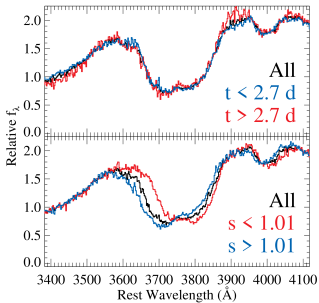
Figure 1: Median spectra from the M12 sample. The black curve is the median spectrum from their full sample. In the top panel, the blue and red curves represent the median spectra taken from early and late subsamples, respectively, while in the bottom panel, they represent low and high stretch (corresponding to low and high luminosity) subsamples, respectively.

We also generated median spectra for subsets of the full sample. First, we split the sample by phase. Since the velocity of SN features typically decreases monotonically with time because of the receding photosphere, one expects lower velocity features at later times. The phase-split median spectra do not appear to be significantly different from each other or the median spectrum from the full sample. This is likely the result of the M12 sample having a very narrow phase range.

We also split the sample by light-curve shape. We split the sample by $s=1.01$ to match what was done by M12. Here, we see the same result that M12 found and shows in their Figures 5 and 7. Namely, the low-stretch (corresponding to faster-declines and lower luminosity) SNe have narrower, seemingly lower velocity features than those of high-stretch SNe.

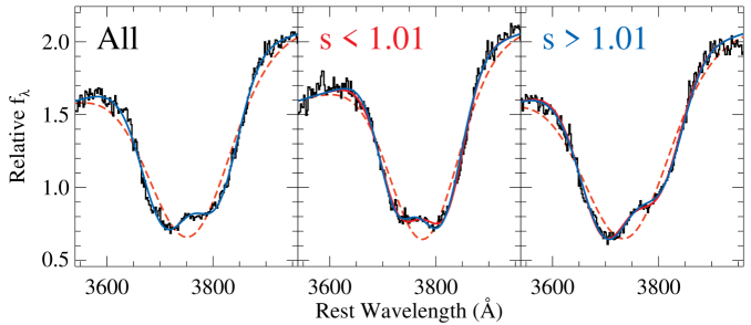
Figure 2: Median spectra from the M12 sample. The left, center, and right panels show the median spectra from the full sample, the low-stretch subsample, and the high-stretch subsample, respectively. The blue and red curves are double-Gaussian fits to the data. The blue curve in the left panel and the red curves in the middle and right panels are the best fits with all parameters allowed to vary. The blue curves in the middle and right panels represent fits where the centroid and width of the redder Gaussian were fixed to the best-fitting values for the full sample. The orange dashed curves are single-Gaussian fits.

Given the above difference, it is worth a detailed look at the line profiles. Despite coming from P-Cygni profiles, the line profiles appear to be similar to the sum of two Gaussians, and performing such a fit resulted in excellent matches to the profiles. The absorption component of a P-Cygni profile is very similar to a Gaussian, so using Gaussians to fit the absorption is a reasonable choice. In Figure 2, we display the median spectra for the full sample and the low/high-stretch subsamples. We also display the best-fitting double-Gaussian fits (after removing a linear pseudo-continuum) to each line profile. For each case, we performed a six–parameter fit, allowing the centroid, width, and height of each Gaussian to vary. The centroid of each Gaussian corresponds roughly to the characteristic velocity of that component. Similarly, the width of each feature corresponds to the velocity-width of the absorbing region for that feature. Finally, the height of each feature is roughly related to the amount of absorbing material at a given velocity. The six–parameter double-Gaussian fits to each profile are represented by the blue lines in Figure 2.

We also fit the low/high-stretch subsamples with two parameters fixed and four allowed to vary. The centroid and width (the parameters related to velocity) of the redder Gaussian was fixed to match the best-fitting values for the full-sample median spectrum, and the remaining parameters (all parameters for the bluer Gaussian and the height of the redder Gaussian) were allowed to vary. These fits are represented by the red lines in Figure 2. Visually, the six–parameter fit is not a significantly better representation of the data than the four–parameter fit. The reduced $\chi^{2}$ decreases by 0.10 and 0.06 when changing from the six–parameter to the four–parameter fit for the low and high-stretch subsamples, respectively. That is, the four–parameter fit has a smaller reduced $\chi^{2}$ than the six–parameter fit (although only marginally smaller), and thus, the subsamples and the full sample are completely consistent with all having the same velocity for the red component.

M12 argued that the difference in the red edge of the Ca H&K line profile was evidence that the subsamples have different ejecta velocities. But we have shown that simply varying the height of the redder Gaussian (and the bluer Gaussian) are sufficient to produce the red edge of the profile. That is, the apparent different in the red edge can be explained by different line strengths rather than different line velocities, and thus a difference in the red edge is not sufficient to distinguish different velocity features.

We also attempted to fix the parameters of the bluer Gaussian, but that did not result in good fits. From these tests, we see that (1) the red component does not necessarily have a different centroid (and thus velocity) for the two subsamples and (2) the blue component does have a different centroid.

We now turn to the difficulty of reducing these profiles to a single parameter, namely velocity. There have been two approaches to measure velocities. The first fits a single Gaussian to a line profile and ascribes the centroid of the Gaussian to the velocity of the feature. This method is used by many studies, including M12. The alternative is to measure the wavelength of maximum absorption (usually after some smoothing) to represent the velocity of the feature. This is the method described by Blondin et al. (2006) and used by Foley et al. (2011) and Foley (2012). Although there are many arguments to use either method, we will focus on the potential systematic errors of using these methods when a feature has multiple components like the Ca H&K feature.

In Figure 2, we also show a single-Gaussian fit to the Ca H&K feature. Besides being a poor representation of the data, the centroid of the Gaussian is consistently intermediate to the two components. Usually, one wants to measure the photospheric velocity for a given feature. With that goal, the single Gaussian clearly fails. A single Gaussian, by measuring something intermediate to the two components, measures nothing physical. Furthermore, the centroid of the single Gaussian is significantly affected by the blue component. The single Gaussian fits for the subsamples indicate that the low-stretch SNe have significantly lower velocities than the high-stretch SNe. However, the double-Gaussian fits show that this is not the case for the photospheric component.

To investigate the importance of the blue component to the measured $v_{\rm Ca\,H\&K}$ from these two methods, we created artificial, but realistic, line profiles. In Figure 3, we again show the median spectrum from the M12 sample. We created a double-Gaussian line profile to mimic the profile of the median spectrum. We then varied the height of the bluer Gaussian, but left all other parameters fixed. We display several example line profiles in Figure 3. Visually, all of these line profiles appear physically possible and represented in nature. The full sample of line profiles vary from having no blue component to having a blue component that is about twice as strong as the red component.

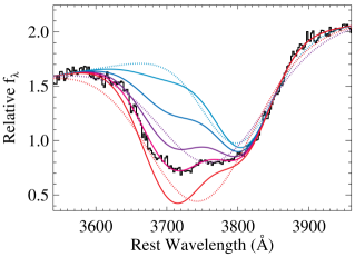
Figure 3: Ca H&K line profiles. The black curve is the median spectrum from the full M12 sample. The solid lines are artificial line profiles created from two Gaussians where only the height of the blue component varies. The dotted lines are single-Gaussian fits to the artificial profiles.

We fit single Gaussians to all artificial line profiles. We display a subset of these fits in Figure 3 (those that match the subset of profiles displayed). As expected, the stronger the blue component, the bluer the centroid of the Gaussian. In Figure 4, we show the measured $v_{\rm Ca\,H\&K}$ from these Gaussian fits. Over the range we explore (from no blue component to a blue component that is twice as strong as the red component), the measured $v_{\rm Ca\,H\&K}$ changes by more than 5000  km s^-1. Even when the blue component is about a third as strong as the red component, the measured $v_{\rm Ca\,H\&K}$ is $\sim\!\!$ 1000  km s^-1 different from the true $v_{\rm Ca\,H\&K}$.

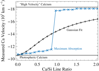
Figure 4: Measured velocity for artificial line profiles. The horizontal black lines represent the velocity of the two components (as measured from their centroid and assuming a rest wavelength of 3945 Å), with the lower and higher velocity components labelled “Photospheric Calcium” and “‘High Velocity’ Calcium,” respectively. The black crosses represent the measured $v_{\rm Ca\,H\&K}$ from a single Gaussian to fit the profiles. The blue X’s represent the measured $v_{\rm Ca\,H\&K}$ from the wavelength of maximum absorption.

We also measured the wavelength of maximum absorption. This wavelength is associated with the blue component when it is stronger and quickly transition its association to the red component as the blue component becomes weaker. The measured $v_{\rm Ca\,H\&K}$ for our artificial line profiles is shown in Figure 4. Although this method fails dramatically for strong blue components, the measured $v_{\rm Ca\,H\&K}$ is relatively constant for line ratios less than one, with all measured velocities $<$1000  km s^-1 for all such cases. There is a slight bias ($\sim\!\!$ 150  km s^-1) for these measurements, some of which can be explained by increasing flux of the pseudo-continuum with wavelength. Correcting for the pseudo-continuum removes much of the bias, with the remaining bias related to the strength of the blue component.

For cases where the red component is stronger than the blue component, measuring the wavelength of maximum absorption is significantly better at measuring the photospheric velocity than using a Gaussian fit to the full profile. In this regime, the wavelength of maximum absorption is only minimally affected by the strength of the blue component, while the Gaussian fit is significantly affected. In the regime of having a stronger blue component, the wavelength of maximum absorption fails. However, in this regime, the Gaussian fit also fails, producing unphysical and significantly biased results.

Using the Foley et al. (2011) method of culling $v_{\rm Ca\,H\&K}$ measurements that are not representative of the photospheric velocity, one should have reliable $v_{\rm Ca\,H\&K}$ measurements, but will necessarily have an incomplete sample. A potential way to avoid this bias would be to perform a double-Gaussian fit. We have not investigated how this method performs with noisy data.

3 SYNOW Models

To further understand the nature of the Ca H&K feature, we use the SN spectrum-synthesis code SYNOW (Fisher et al., 1997) to create simple SYNOW spectral models. We specifically use these models to test how temperature can affect the profile and look for trends between the Ca H&K profile shape and other spectral features. Although SYNOW has a simple, parametric approach to creating synthetic spectra, it can provide insight on basic trends in SN SEDs. To generate a synthetic spectrum, one inputs a blackbody temperature ($T_{\rm BB}$), a photospheric velocity ($v_{\rm ph}$), and for each involved ion, an optical depth at a reference line, an excitation temperature ($T_{\rm exc}$), the maximum velocity of the opacity distribution ($v_{\rm max}$), and a velocity scale ($v_{e}$). This last variable assumes that the optical depth declines exponentially for velocities above $v_{\rm ph}$ with an $e$-folding scale of $v_{e}$. The strengths of the lines for each ion are determined by oscillator strengths and the approximation of a Boltzmann distribution of the lower-level populations with a temperature of $T_{\rm exc}$.

We produced models consisting of only Ca ii and with only Si ii and Ca ii to isolate their affect on the profile of the Ca H&K feature. For all models, we set $T_{\rm BB}=10000$ K, $v_{\rm ph}=10000$  km s^-1, $v_{\rm max}=80000$  km s^-1, and $v_{e}=3000$ (for Si ii) and 2000  km s^-1 (for Ca ii). We chose $\tau=5$ and 4 for Si ii and Ca ii, respectively. These parameters were chosen such that when $T_{\rm exc}=10000$ K, the model Ca H&K line profile was visually similar to that of the median spectrum of the M12 sample. Keeping all other parameters fixed, we varied $T_{\rm exc}$ from 5000 to 20000 K. A subset of the models spanning this range are presented in Figure 5.

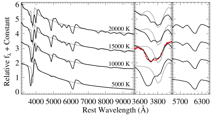
Figure 5: SYNOW model spectra. The dashed and solid curves represent models including only Ca ii and both Si ii and Ca ii, respectively. The models only vary in their excitation temperature, which is labelled. The middle and left panels show detailed views of the Ca H&K feature and the redder Si ii complex, respectively. The median spectrum from the M12 sample is shown in the middle panel to demonstrate that the $T_{\rm exc}=10$,000 K model has a similar Ca H&K profile shape.

As seen in Figure 5, the inclusion of Si ii dramatically changes the Ca H&K profile shape, making it stronger, broader, and bluer. Although the Si ii $\lambda 3858$ feature may be stronger in the models than in real SN spectra, the Si ii $\lambda 6355$ and the Ca H&K features appear to have reasonable strengths.

There is a clear spectral progression as the temperature changes. We note that for SYNOW, $T_{\rm bb}$ only changes the continuum shape of the models and does not affect the strength of features. Since SYNOW uses Ca H&K as the reference calcium line, the strength of the Ca H&K absorption by definition does not change much with $T_{\rm exc}$, and the entire calcium spectrum does not change much over the temperatures probed. Meanwhile the Si ii spectrum changes significantly with varying $T_{\rm exc}$. The strength of the Ca H&K absorption within the Ca H&K feature (i.e., the strength of the red component) does change slightly with $T_{\rm exc}$ because of the strength of the Si ii $\lambda 3858$ emission changing the apparent Ca H&K absorption.

In the red, there is the expected change in the ratio of the Si ii $\lambda 5972$ and $\lambda 6355$ lines. This ratio, $\mathcal{R}$(Si), is highly correlated with luminosity and light-curve shape (Nugent et al., 1995). As the Si ii $\lambda 5972$ feature becomes stronger, the Si ii $\lambda 3858$ feature becomes weaker. For the SYNOW models, $\mathcal{R}$(Si) increases with increasing $T_{\rm exc}$, while for SNe Ia, $\mathcal{R}$(Si) increases with decreasing $T$; this has been previously noted (e.g., Bongard et al., 2008), and is likely the result of not simultaneously changing the opacity with $T_{\rm exc}$ and/or non-local thermodynamic equilibrium effects. However, the Ca ii spectrum does not change significantly with $T_{\rm exc}$ and other model spectra show the same relation between Si ii $\lambda 3858$ and Si ii $\lambda 5972$ (e.g., Kasen & Plewa, 2007; Blondin et al., 2012a). We therefore consider the qualitative changes in the spectra to be correct, although the corresponding temperatures may not be. All models show that the strength of Si ii $\lambda 3858$ and Si ii $\lambda 5972$ are anti-correlated; we will use this relation as the primary model prediction. We will later use $\mathcal{R}$(Si) as a proxy for light-curve shape.

The excitation energy for the various Si ii lines also explain the correlations between the various Si ii features. The Si ii $\lambda 3858$, Si ii $\lambda 5972$, and Si ii $\lambda 6355$ features have excitation energies of 6.9, 10.0, and 8.1 eV, respectively. Because the Si ii $\lambda 3858$ and Si ii $\lambda 5972$ features have very different excitation energies and Si ii $\lambda 6355$ has an excitation energy intermediate to the other two features, the strengths of the Si ii $\lambda 3858$ and Si ii $\lambda 5972$ features should change in opposite directions with changing temperature. This also explains the SYNOW results since SYNOW fixes the strength of the reference feature, Si ii $\lambda 6355$.

In the middle and right-hand panels of Figure 5, we show the Ca H&K feature and redder Si ii complex in detail. Again, it is clear that both $\mathcal{R}$(Si) and the strength of the Si ii $\lambda 3858$ feature change in the way described above.

A SN photosphere is, of course, more complicated than the simple SYNOW model. Specifically, as the temperature changes over the relevant range, the ionization of silicon (specifically the amount of singly and doubly ionized silicon) changes. Additionally, certain features may be saturated (and possibly for only certain temperatures). Specifically, it is thought that Si ii $\lambda 6355$ is usually saturated. However, it seems unlikely that the other Si ii features are saturated. Therefore, these additional complexities should not change our interpretation that the strengths of the Si ii $\lambda 3858$ and Si ii $\lambda 5972$ features are anti-correlated and change with temperature.

We fit the Si ii $\lambda 4130$, $\lambda 5972$, and $\lambda 6355$ features in each model spectrum with single Gaussians. Although the line profiles are not exactly Gaussian, the fits are reasonable approximations of the data, and the process is similar to what is done in practice. We also fit the Ca H&K feature with both a single Gaussian and a double Gaussian. We show the measured velocity in Figure 6.

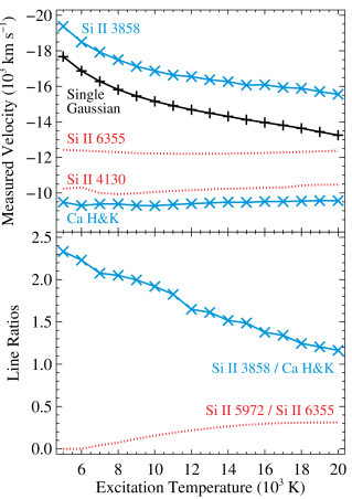
Figure 6: Top Panel: Measured velocity as a function of excitation temperature for SYNOW model spectra. The red dotted lines represent the velocities measured with a single Gaussian for the Si ii $\lambda 4130$ and $\lambda 6355$ lines. The black crosses represent velocities measured with a single-Gaussian fit to the Ca H&K feature. The blue X’s represent velocities measured with a double-Gaussian fit to the Ca H&K feature, where the Si ii $\lambda 3858$ velocity is measured assuming its rest wavelength is 3945 Å. Bottom Panel: The $\mathcal{R}$(Si) (red dotted line) and Si/Ca (blue X’s) line ratios as a function of excitation temperature for the SYNOW model spectra.

The measured Si ii $\lambda 4130$, and $\lambda 6355$ velocities differ by at most 530 and 220  km s^-1 over the entire temperature range, respectively. At the lowest $T_{\rm exc}$, the Si ii $\lambda 5972$ feature is not strong enough to measure a reliable velocity, but for the other temperatures, it differs by at most 440  km s^-1. These differences are encouraging since the photospheric velocities did not change.

Fitting two Gaussians to the Ca H&K feature, which should be better at recovering the true velocity (see Section 2), we see that the red component, corresponding to Ca H&K, has a measured velocity range similarly small to that of the Si ii features noted above. Specifically, the maximum difference of measured Ca H&K velocities over all temperatures probed is only 290  km s^-1. However, the measured velocity for the Si ii $\lambda 3858$ feature changes significantly with temperature. Over the full temperature range probed, the measured Si ii $\lambda 3858$ velocity ranges from $-15$,550 to $-19,$380  km s^-1 – a difference of 3820  km s^-1, or roughly an order of magnitude greater than that of the other features.

A single-Gaussian fit performs even worse. Because of the changing Si ii $\lambda 3858$ velocity and its varying strength, a single-Gaussian fit to the Ca H&K feature results in a $v_{\rm Ca\,H\&K}$ range of $-13$,250 to $-17,670$  km s^-1 over our chosen temperature range for a maximum difference of 4420  km s^-1. Since the $v_{\rm Ca\,H\&K}$ measured using a single Gaussian can have dramatic differences even when there is no change in physical velocities, this is even more reason to avoid this technique.

Figure 6 also shows the Si ii $\lambda 5972$ to Si ii $\lambda 6355$ ($\mathcal{R}$(Si)) and Si ii $\lambda 3858$ to Ca H&K ratios, which we will call the Si/Ca ratio. The range for $\mathcal{R}$(Si), from effectively zero (when Si ii $\lambda 5972$ is difficult to discern) to $\sim\!\!$ 0.3, is approximately the range seen by all SNe Ia except SN 1991bg-like objects (e.g., Blondin et al., 2012b; Silverman et al., 2012). The Ca/Si ratio has a range of 1.2 to 2.3. The ratio is affected by both the strength of the Si ii $\lambda 3858$ absorption and the Si ii $\lambda 3858$ emission, which fills in some of the Ca H&K absorption. As noted above, the strength of the Si ii $\lambda 3858$ feature can have a large affect on the Ca H&K line profile, and even dominates for many temperatures.

Since Si ii $\lambda 5972$ and $\lambda 6355$ do not show significant velocity differences with temperature, are relatively free of contamination from other species, and $\mathcal{R}$(Si) is a good indication of light-curve shape, we can use it as a proxy for light-curve shape for our models. Figure 7 shows $v_{\rm Ca\,H\&K}$ measured with a single Gaussian as a function of $\mathcal{R}$(Si). The measured $v_{\rm Ca\,H\&K}$ decreases in amplitude with increasing $\mathcal{R}$(Si), which corresponds to decreasing stretch and luminosity.

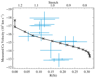
Figure 7: Velocities measured with a single-Gaussian fit to the Ca H&K feature as a function of $\mathcal{R}$(Si) for the SYNOW model spectra. The M12 data are also plotted in blue where the measured stretch is converted to $\mathcal{R}$(Si) with the top axis showing the scaling.

Converting stretch to $\mathcal{R}$(Si), we can plot the M12 measurements on Figure 7. The M12 spectra do not cover the redder Si ii features, so a direct measurement could not be made. The M12 values, which use a single Gaussian to fit the Ca H&K feature, span a similar range of $v_{\rm Ca\,H\&K}$ and inferred $\mathcal{R}$(Si) as the models, with the model trend going through the middle of the data values. The claimed trend of $v_{\rm Ca\,H\&K}$ with light-curve shape is clear using the M12 values. However, this trend is similar to the trend generated by simply changing the temperature in the SYNOW models. We emphasize that the true $v_{\rm Ca\,H\&K}$ is fixed for all models and the $v_{\rm Ca\,H\&K}$ measured using a double-Gaussian fit varies only slightly over all models. The trend shown in Figure 7 is solely the result of the method for measuring the velocity. The underlying physical effect is the changing strength of Si ii $\lambda 3858$ with temperature, and thus light-curve shape.

There will undoubtedly be a true range of velocities in the data. We have not explored how the SYNOW models change when varying several parameters, but it is clearly possible to reproduce the M12 trend through a combination of single Gaussian fitting, an inherent velocity range, and relations between the Ca H&K profile shape with temperature and velocity.

4 The M12 Sample

With the insights of the above analysis, we re-analyse the individual M12 spectra. In Section 2, we showed that fitting the Ca H&K profile with a single Gaussian results in an imprecise, biased, and unphysical measurement of the photospheric velocity. Instead, we fit the Ca H&K profiles of the M12 spectra with two Gaussians. As suggested above, this method should provide relatively unbiased measurements of the Si ii $\lambda 3858$ feature and the Ca H&K feature.

We provide the best-fitting velocities for Si ii $\lambda 3858$ assuming that it is “HV” Ca H&K and Ca H&K in Table 1. We also provide the Si/Ca ratio in Table 1.

Figure 8 compares the velocities measured with the double-Gaussian fit to those reported by M12. The $v_{\rm Ca\,H\&K}$ is systematically lower than the M12 value for the same SNe. Similarly, the Si ii $\lambda 3858$ (when treated as HV Ca H&K) is systematically higher than the M12 value for the same SNe. Performing a Bayesian Monte-Carlo linear regression on the M12–Si ii and M12–Ca H&K data sets (Kelly, 2007), we find that 99.8 and 86.8 per cent of the realizations have positive slopes, respectively, corresponding to 3.1-$\sigma$ and 1.5-$\sigma$ results, respectively. That is, there is significant evidence for a linear relation between the M12 $v_{\rm Ca\,H\&K}$ measurements and the Si ii $\lambda 3858$ velocity, but no evidence for a linear relation between the M12 $v_{\rm Ca\,H\&K}$ measurements and the velocity of the red component corresponding to absorption from photospheric calcium.

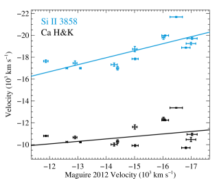
Figure 8: M12 Ca H&K velocities measured using a single-Gaussian fit to the Ca H&K feature compared to velocities measured with a double-Gaussian fit to the Ca H&K feature for the M12 sample. The black and blue points represent the Ca H&K and Si ii $\lambda 3858$ (assuming a rest wavelength of 3945 Å) velocities from the double-Gaussian fit. The solid lines represent the best-fitting linear relationships for the data, corresponding to 1.5 and 3.1-$\sigma$ results for Ca H&K and Si ii $\lambda 3858$, respectively.

As expected from the results of Section 3, the M12 $v_{\rm Ca\,H\&K}$ measurements are intermediate to the Si ii $\lambda 3858$ and Ca H&K velocities, more closely track the Si ii $\lambda 3858$ velocity than the Ca H&K velocity, and are systematically biased measurements of $v_{\rm Ca\,H\&K}$.

For much of the analysis performed by M12, they corrected their measured $v_{\rm Ca\,H\&K}$ to a maximum-light value, $v_{\rm Ca\,H\&K}^{0}$, using a single velocity gradient for all objects derived from the $v_{\rm Ca\,H\&K}$ and effective phase measurements for their sample. Using a large sample where many objects had multiple spectra obtained near maximum light, Foley et al. (2011) showed that $v_{\rm Ca\,H\&K}^{0}$ and the velocity gradient were highly correlated with higher-velocity SNe also having higher-velocity gradients. Taking into account this relation, they produced an equation which estimates $v_{\rm Ca\,H\&K}^{0}$ given $v_{\rm Ca\,H\&K}$ and phase. Using the M12 velocity gradient results in differences between $v_{\rm Ca\,H\&K}$ and $v_{\rm Ca\,H\&K}^{0}$ that can be as large as 1150  km s^-1, and the median difference is 460  km s^-1. However, if one uses the Foley et al. (2011) relation to correct the velocity measurements to have a common phase of 2.7 d (the median of the sample), then the deviation between that value and $v_{\rm Ca\,H\&K}$ is at most 560  km s^-1, with a median absolute deviation of 120  km s^-1, both of which are smaller than the typical uncertainty of 670  km s^-1 for the M12 $v_{\rm Ca\,H\&K}^{0}$ measurements. The combination of using a single velocity gradient and extrapolating to maximum light (only one spectrum in the sample has a phase before maximum brightness) introduces unnecessary additional uncertainty. Instead in all further analysis, we use the raw $v_{\rm Ca\,H\&K}$ measurements, but add an additional 120  km s^-1 uncertainty in quadrature to the reported uncertainty.

Using our measurements of $v_{\rm Ca\,H\&K}$, we can re-examine the M12 claim that $v_{\rm Ca\,H\&K}$ is correlated with light-curve shape. In Figure 9, we show the Si ii $\lambda 3858$, Ca H&K, and M12 velocity measurements as a function of stretch. This figure is similar to Figure 7.

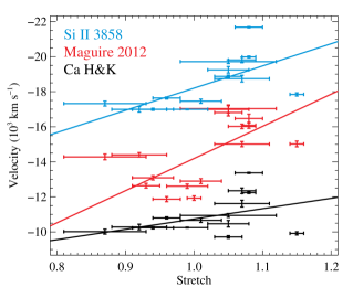
Figure 9: Velocities measured with a single or double-Gaussian fit to the Ca H&K feature as a function of stretch for the M12 sample. The single-Gaussian measurements are taken from M12 and represented by the red data. The double-Gaussian measurements are shown as black and blue points for the Ca H&K and Si ii $\lambda 3858$ (assuming a rest wavelength of 3945 Å) components, respectively. The solid lines represent the best-fitting linear relationships for the data, corresponding to 2.3, 2.3, and 1.4-$\sigma$ results for the M12, Si ii $\lambda 3858$, and Ca H&K velocities, respectively.

Performing a Bayesian Monte–Carlo linear regression on the M12, the Si ii $\lambda 3858$, and Ca H&K velocity measurements, we find that 97.7, 97.8, and 87.6 per cent of the realizations have positive slopes, respectively, corresponding to 2.3-$\sigma$, 2.3-$\sigma$, and 1.5-$\sigma$ results, respectively. We therefore find mild evidence that the M12 and Si ii $\lambda 3858$ velocity measurements are linearly related to stretch. We find no statistical evidence that $v_{\rm Ca\,H\&K}$ is linearly related to stretch.

M12 found a 3.4-$\sigma$ linear relation between their $v_{\rm Ca\,H\&K}^{0}$ measurements and stretch. Above, our measured significance is much lower. This is partly because in the above calculation, we did not include SNe 2011by and 2011fe since we do not have the M12 spectra. Including the reported values for these SNe, there is only a minor change in the significance, changing the percentage of realizations with positive slopes to be 98.7 per cent, which is a 2.5-$\sigma$ result. The other difference is that above we examine $v_{\rm Ca\,H\&K}$ instead of $v_{\rm Ca\,H\&K}^{0}$. Performing the same analysis as M12 (using $v_{\rm Ca\,H\&K}^{0}$ and including SNe 2011by and 2011fe), we find that 99.4 per cent of the realizations have positive slopes, which is a 2.8-$\sigma$ result. The difference in significance is likely in the subtleties of fitting a line. This practice is not trivial (Hogg, Bovy, & Lang, 2010), but the Kelly (2007) method is generally a better choice than most options.

We also performed a Kolmogorov–Smirnov (KS) test, splitting the samples by a stretch of 1.01. This is not an ideal test since there are several SNe with stretches consistent with 1.01 (and therefore could be in either group) and uncertainty in the velocity can also change the overall distribution, but it can provide an indication of a difference. The KS test resulted in $p$ values of 0.0014, 0.0036, and 0.080 for the M12, the Si ii $\lambda 3858$, and Ca H&K velocity measurements, respectively. These tests indicate that the low and high-stretch subsamples have different parent populations for both the Si ii $\lambda 3858$ and M12 velocities. However, there is no statistical evidence that the low/high-stretch subsamples have different parent $v_{\rm Ca\,H\&K}$ distributions.

Although there is only marginal evidence that there is a linear relationship between the M12 measurements and stretch, we find a similar significance of a relationship between Si ii $\lambda 3858$ velocity and stretch. Since the $v_{\rm Ca\,H\&K}$ shows no evidence for a correlation with stretch and the M12 measurements are correlated with the Si ii $\lambda 3858$ velocity (and at most weakly correlated with the Ca H&K velocity), the physical relationship underlying the result identified by M12 is likely the correlation between Si ii $\lambda 3858$ velocity and stretch. From the SYNOW models, this relation is understood as a temperature effect (and not a real difference in photospheric velocity).

Next, we examine the Si/Ca ratio. We show the Si/Ca ratio as a function of stretch for the M12 sample in Figure 10. Performing a Bayesian Monte–Carlo linear regression on the data, we find that 82.4 per cent of the realizations have positive slopes, corresponding to a 1.4-$\sigma$ result. Although there is no evidence for a linear relationship between stretch and the Si/Ca ratio in the M12 data, there is a slight correlation with higher stretch SNe having larger Si/Ca ratios. This is the same general trend expected from the SYNOW models, and future investigations should determine if such a trend exists.

Figure 10: Si/Ca ratio as a function of stretch for the M12 sample. The solid line represents the best-fitting linear relationship for the data, corresponding to a 1.4-$\sigma$ result.

Finally, we compare the Si/Ca ratio to our measured velocities (Figure 11). There are no obvious trends (1.0 and 1.7-$\sigma$) between the Si/Ca ratio and the Si ii $\lambda 3858$ or Ca H&K velocities. However, there is a moderate trend between the Si/Ca ratio and the M12 measurements (2.7-$\sigma$), where the M12 velocities increase with increasing Si/Ca ratio. One should expect that the single-Gaussian method (as employed by M12) should be intermediate to the Si ii $\lambda 3858$ and Ca H&K velocities. The velocity should be closer to the Ca H&K velocity when the Si ii $\lambda 3858$ feature is weak (small Si/Ca ratio) and closer to the Si ii $\lambda 3858$ velocity when the feature is strong (large Si/Ca ratio).

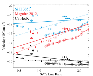
Figure 11: Velocities measured with a single or double-Gaussian fit to the Ca H&K feature as a function of the Si/Ca ratio for the M12 sample. The single-Gaussian measurements are taken from M12 and represented by the red data. The double-Gaussian measurements are shown as black and blue points for the Ca H&K and Si ii $\lambda 3858$ (assuming a rest wavelength of 3945 Å) components, respectively. The solid lines represent the best-fitting linear relationships for the data, corresponding to 2.7, 1.0, and 1.7-$\sigma$ results for the M12, Si ii $\lambda 3858$, and Ca H&K velocities, respectively. The dotted lines represent the best-fitting linear relationships for the data with a Si/Ca ratio of $>$1. The red, black, and blue circles represent the single-Gaussian and double-Gaussian fit velocities for the SYNOW model spectra.

The behavior seen in the data is reproduced to some extent by the SYNOW models. Figure 11 also shows the SYNOW model Si/Ca ratio compared to the Si ii $\lambda 3858$, Ca H&K, and single-Gaussian velocities. The Ca H&K velocity is relatively flat for the SYNOW models, while the Si ii $\lambda 3858$ and single-Gaussian velocities increase with increasing Si/Ca ratio. The Ca H&K and single-Gaussian trends are similar in the data and models, but the data have higher velocities than the data (by about 700 and 2200  km s^-1, respectively). There is no obvious trend in the Si ii $\lambda 3858$ data, contrary to what is seen in the models.

The models are restricted to Si/Ca ratios of $>$1. If we fit the data with the same restriction, the fits are more similar to the slopes seen in the models. Specifically, the trend with Ca H&K is flatter and the trend with Si ii $\lambda 3858$ is stronger, although neither trend is statistically significant. Perhaps a simple linear relation is not sufficient to describe the trend between the Si/Ca ratio and Si ii $\lambda 3858$ velocity.

5 The CfA Sample

Although the M12 sample was used to identify some trends which were investigated above, it is limited in size. To test additional trends, we use the CfA spectral sample (Blondin et al., 2012b). Over the last two decades, the CfA SN Program has observed hundreds of SNe Ia, mostly with the FAST spectrograph (Fabricant et al., 1998) mounted on the 1.5 m telescope at the F. L. Whipple Observatory. The data have been reduced in a consistent manner (Matheson et al., 2008; Blondin et al., 2012b), producing well-calibrated spectra. These spectra often cover Ca H&K and always cover Si ii $\lambda 6355$, which the M12 spectra do not cover.

For SNe Ia in the sample with a measured time of maximum brightness from light curves, $v_{\rm Si~{}II}$ and $v_{\rm Ca~{}H\&K}$ have been measured (Blondin et al., 2012b). Briefly, this is achieved by first generating a smoothed spectrum using an inverse-variance Gaussian filter (Blondin et al., 2006), and the wavelength of maximum absorption in the smoothed spectrum is used to determine the velocity (see Blondin et al. 2012b for details). The measurements for each spectrum have been reported by Foley et al. (2011), and measurements in all cases were obtained by Blondin et al. (2012b)

The CfA sample contains 1630 $v_{\rm Si~{}II}$ and 1192 $v_{\rm Ca~{}H\&K}$ measurements for 255 and 192 SNe Ia, respectively.

The velocity of each absorption minimum in the Ca ii H&K feature of the smoothed spectra is automatically recorded (Blondin et al., 2012b). We only examine spectra with one or two minima. If two minima are found, the higher/lower velocities are classified as “blue”/“red.” If only one minimum is found, it is categorized as the red or lower-velocity component.

Foley et al. (2011) noted that comparing all $v_{\rm Ca~{}H\&K}$ measurements to their corresponding $v_{\rm Si~{}II}$ measurements, there were two distinct “clouds” corresponding to a lower and higher velocity relative to $v_{\rm Si~{}II}$. The higher-velocity cloud typically corresponds to the blue velocity component, although there are some red measurements in that cloud. The red measurements in the blue cloud typically have indications of a lower-velocity component, such as a red shoulder in the line profile, and it was assumed that they likely corresponded to measurements which were physically similar to the blue measurements and were simply misclassified.

In Figure 12, we show the subset of CfA measurements of spectra with $-1\leq t\leq 4.5$ d (chosen to match the M12 sample). This subset also shows the distinct blue/red clouds. We used the method of Williams, Bureau, & Cappellari (2010) to fit a single slope, but separate offsets to the two clouds. As a result of that fitting, there is a natural dividing line between the two clouds, and we used this line to produce cleaner subsamples. We removed every blue measurement in the red cloud, since they may be errant measurements. We also reassigned every red measurement in the blue cloud as a “blue” measurement because of the reasons listed above. This full process is shown graphically in the three panels of Figure 12.

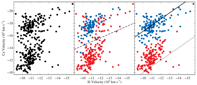
Figure 12: Velocities from the Ca H&K profile (both blue and red components), assuming a rest wavelength of 3945 Å, as a function of Si ii $\lambda 6355$ velocity for the CfA sample with a phase range of $-1\leq t\leq 4.5$ d. The middle panel plots the data as blue and red for the blue and red components, respectively. The dashed line represents the line of separation for the two clouds from the fitting method of Williams et al. (2010). The right panel removes all measurements from blue components in the red cloud (as determined by the dividing line) and assigns all “red” velocities in the blue cloud as “blue” points under the assumption that they were originally misclassified. The dotted line represents spectra that would have the same Ca H&K and Si ii $\lambda 6355$ velocities. The solid line represents spectra that would have the same Ca H&K and Si ii $\lambda 6355$ velocities if Ca H&K were actually from Si ii $\lambda 3858$ absorption at the same velocity as Si ii $\lambda 6355$.

With these clean subsets, we have a reasonable estimate of the velocities for the blue and red components of the Ca H&K feature. Since some SNe in the CfA sample have multiple spectra in the chosen phase range, we created samples for each velocity group where there is one measurement per SN. For each SN, we chose the measurement closest to a phase of $t=2.7$ d, the median of the M12 sample. This resulted in samples of 66 and 67 SNe Ia with blue and red measurements (approximately one-third of the full CfA sample and about 5 times as large as the M12 sample), respectively. We present those measurements as a function of light-curve shape (specifically, $\Delta m_{15}(B)$) in Figure 13. There is no significant linear relation between light-curve shape and the individual velocity components. In fact, the stronger relationship of the red velocity component, which is the best representation of the Ca H&K photospheric velocity, is a 1.3$\sigma$ result in the opposite direction than the M12 relation (i.e., higher velocity for slower-declining SNe Ia). Because of this opposing trend, the CfA data are significantly inconsistent with the M12 relation. However, this result is consistent with that of Foley et al. (2011) and Foley (2012) for both Ca H&K and Si ii $\lambda 6355$.

Figure 13: Velocity of the blue (top) and red (bottom) components of the Ca H&K profile (assuming a rest wavelength of 3945 Å) vs. $\Delta m_{15}(B)$ for the CfA sample and a phase range of $-1\leq t\leq 4.5$ d. The choice of blue and red velocities were made as described in the text and visually represented in Figure 12. Each point represents a different SN (66 and 67, respectively). There is no significant correlation for either (linear relations are 0.4$\sigma$ and 1.3$\sigma$ significant, respectively). Since the red component, corresponding to photospheric Ca H&K, has a slight (but insignificant) trend of higher velocity with faster-declining light curves, the data are significantly inconsistent with the claim of M12 that Ca H&K velocity decreases with faster-declining light curves.

In addition to the arguments detailed above, there is additional evidence in the CfA data that suggest that the blue component of the Ca H&K feature is the result of Si ii $\lambda 3858$. If the blue component is predominantly from HV Ca H&K, then one would not expect a particularly high correlation between its velocity and that of Si ii $\lambda 6355$. That is, the velocity of a HV calcium component could be independent of the photospheric silicon velocity. However, there is a reasonable correlation (correlation coefficient of 0.54) between the two. On the other hand, the velocities of the red and blue components are barely correlated (correlation coefficient of 0.27). Therefore, the velocity of the blue component has a larger association with the photospheric velocity of silicon than the photospheric velocity of calcium.

Perhaps the best evidence that the blue component is from Si ii $\lambda 3858$ absorption is presented in Figure 12. In the right panel, we plot the relation between $v_{\rm Si\,II}$ and $v_{\rm Ca\,H\&K}$ in the scenario where the $v_{\rm Ca\,H\&K}$ measurement is from a misidentified Si ii $\lambda 3858$ feature at the same velocity as Si ii $\lambda 6355$. The line goes directly through the blue cloud, indicating that the blue component of the Ca H&K feature has a velocity consistent with that of Si ii $\lambda 6355$ if it is formed by Si ii $\lambda 3858$ absorption. In other words, the blue component is at the wavelength one expects by blueshifting 3858 Å by $v_{\rm Si\,II}$. Addtionally, Blondin et al. (2012b) presented several examples of SNe where the blue component was consistent with Si ii $\lambda 3858$ at the Si ii $\lambda 6355$ velocity, while the red component was consistent with the velocity of the Ca NIR triplet.

From the large CfA sample, we showed additional evidence that $v_{\rm Ca\,H\&K}$ does not correlate with light-curve shape. The velocity of the blue component is correlated with the photospheric silicon velocity (as measured by Si ii $\lambda 6355$) and relatively uncorrelated with the photospheric calcium velocity. In addition to being correlated with photospheric silicon velocity, the CfA data show that the velocity of the blue component matches the expected photospheric velocity of Si ii $\lambda 3858$.

6 Additional Modeling

From the above analysis of the SYNOW models, the comparison of the M12 sample to the SYNOW models, and an examination of the CfA sample, there is significant evidence that the blue component of the Ca H&K feature is predominantly from Si ii $\lambda 3858$. However, additional confidence in this claim can be obtained by modeling specific SNe.

In this section, we examine the two possible scenarios for the blue component of the Ca H&K feature (either HV calcium or Si ii $\lambda 3858$) for two test cases: SN 2011fe and SN 2010ae.

6.1 SN 2011fe

SN 2011fe, which occurred in M 101 and was the brightest SN Ia in 40 years, has been incredibly well observed and extensively studied (e.g., Nugent et al., 2011; Brown et al., 2012; Chomiuk et al., 2012; Horesh et al., 2012; Margutti et al., 2012; Matheson et al., 2012; Parrent et al., 2012; Shappee et al., 2013). Here we examine a single maximum-light spectrum of SN 2011fe, obtained by HST using the STIS spectrograph (Program GO–12298; PI Ellis). The spectra were obtained on 2011 September 10 between 09:51 and 11:14 UT, corresponding to $t=0.0$ d relative to $B$-band maximum brightness (M12). The observations were obtained with three different gratings, all with the $52\hbox{${}^{\prime\prime}$}\times 0.\hbox{${}^{\prime\prime}$}2$ slit. Two exposures were obtained for each of the CCD/G230LB, CCD/G430L, and CCD/G750L setups with individual exposure times of 530, 80, and 80 s, respectively. The three setups yield a combined wavelength range of 1665 – 10,245 Å. The data were reduced using the standard HST Space Telescope Science Data Analysis System (STSDAS) routines to bias subtract, flat-field, extract, wavelength-calibrate, and flux-calibrate each SN spectrum.

We present the spectrum in Figure 14. We note that M12 presented a spectrum for SN 2011fe from a different phase and which only covered $\sim\!\!$ 2900 – 5700 Å. This is the first publication of these data. This is also only the second published maximum-light SN Ia spectrum to probe below $\sim\!\!$ 2500 Å (the first being of SN 2011iv; Foley et al. 2012c).

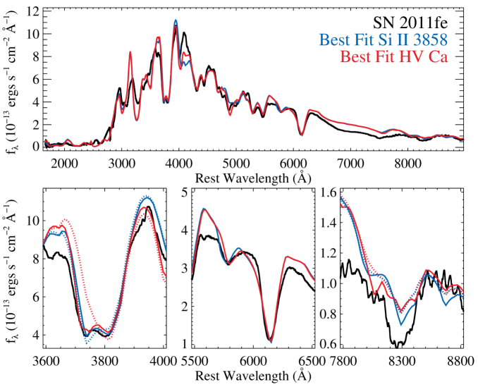
Figure 14: HST spectrum of SN 2011fe at $t=0.0$ d (black curve). The blue and red curves are “best-fitting” SYNOW model spectra where there was an attempt to simultaneously match the Ca H&K profile and Si ii $\lambda 5972$ and $\lambda 6355$ lines using Si ii/HV Ca ii to match the blue component of the Ca H&K feature, respectively, and differences in the strength of Na D to match the Si ii $\lambda 5972$ feature. The dotted red line represents the model represented by the solid red line except without a HV Ca ii component. The dotted blue line represents the model represented by the solid blue line, except with the Ca ii opacity and density structure matched to that of the model represented by the solid red line.

The SN 2011fe spectrum is of extreme high quality, including in the UV. Because of its quality and wavelength coverage, we can produce a reasonable SYNOW model. We have made two attempts at fitting the SN 2011fe spectrum using SYNOW models. The first assumes that the blue component of the Ca H&K feature is from Si ii $\lambda 3858$; the second assumes that it is caused by HV Ca H&K. We present our models in Figure 14 and model parameters in Table 2.

When generating these models, we first attempted to fit the full spectrum with a limited number of species. These models are not optimized to fit the entire spectrum; because of potential effects other species could have on the spectral features of interest, we wanted a first-order model of the full spectrum. We then either added HV Ca ii or adjusted the Si ii temperature to match the blue component of the Ca H&K feature. We allow the opacity and density structures for Ca ii, Si ii, HV Ca ii, and Na i to vary, but all other species remain the same.

For the HV calcium model, we adjusted the Si ii temperature to an extreme value that still fits the Si ii $\lambda 5972$ feature. In this model, we do not include any Na i, and therefore Na D does not contribute at all to this feature. As a result, the Si ii $\lambda 3858$ is about as weak as possible, and the HV Ca H&K is essentially as strong as possible.

For the Si ii $\lambda 3858$ model, we adjust the Si ii temperature to an extreme value to match the blue feature in the Ca H&K feature. We then add Na i to match the strength of the feature near 5800 Å.

These models differ in some ways from those presented by Parrent et al. (2012) for their optical-only maximum-light SN 2011fe spectrum. Most differences are related to matching the UV region, which requires adding Co ii and Cr ii. Interestingly, adding these features reduces the need to include Fe ii in the SYNOW model (although we cannot definitively say that it is not in the spectrum). Additionally, we are able to better model the Ca H&K feature than Parrent et al. (2012) because of the additional data blueward of the feature.

Examining the SYNOW models in detail, particularly near the Ca H&K feature, the redder Si ii features, and the Ca NIR triplet (see lower panels of Figure 14), we see that the models are very similar. In other words, SYNOW modeling of SN 2011fe cannot distinguish between our two scenarios; it simply has too many parameters for the data.

We did not adjust the models to fit the Ca NIR triplet, with the hope that we might see signatures of HV Ca. There is a feature in the SYNOW model that is coincident with a shoulder in the SN 2011fe spectrum. However, we see a similar feature in the Si ii $\lambda 3858$ model that is simply the result of a slightly different density profile for Ca ii. A full spectral sequence and/or NIR spectra, which would supply additional Si ii features, may provide a clear way to distinguish the models.

6.2 SN 2010ae

With an inconclusive result from modeling SN 2011fe, we now turn to modeling SN 2010ae. SN 2010ae is a SN Iax (Foley et al., 2012a) similar to SN 2008ha (Foley et al., 2009, 2010; Valenti et al., 2009). Its spectrum is similar to that of a SN Ia, but with an extremely low ejecta velocity. This indicates that the ejecta composition, density structure, temperature, and other aspects of the explosion important for producing a particular SED are similar for SN 2010ae and SNe Ia. However, because of the low ejecta velocity, line blending is minimal.

We present a near maximum-light spectrum of SN 2010ae originally presented by Foley et al. (2012a) and presumed to be obtained near maximum light in Figure 15. This spectrum only covers optical wavelengths. We dereddened the spectrum by $E(B-V)=0.6$ mag to roughly match the continuum of SN 2011fe and smoothed the spectrum with a inverse-variance weighted Gaussian filter and velocity scale of 150  km s^-1.

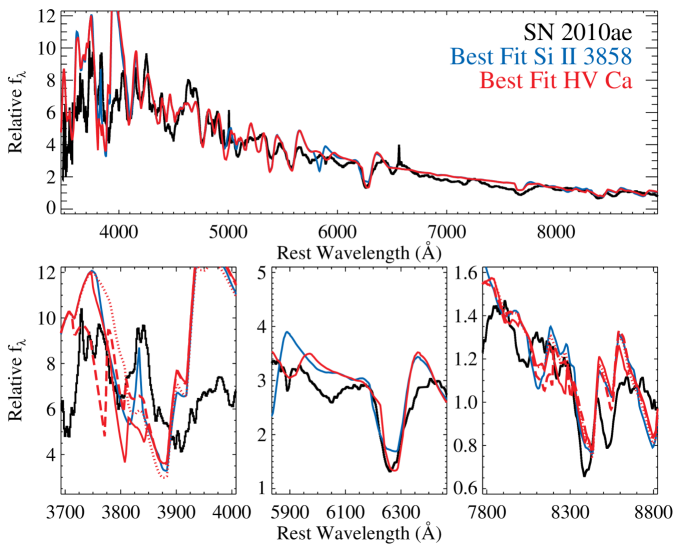
Figure 15: Same as Figure 14, except for SN 2010ae and its “best-fitting” SYNOW models. The SN 2010ae spectrum has been smoothed slightly and dereddened as described in the text. The solid and dashed red lines are for HV calcium where Ca K and Ca H, respectively, are matched to the absorption near 3800 Å.

Perhaps the most important aspect of the SN 2010ae spectrum is that the Ca H&K feature is separated into two distinct features.

We then attempted to produce SYNOW model spectra in a way similar to what was performed for SN 2011fe. As a starting point, we used the SN 2011fe models. We decreased $v_{\rm phot}$ from 9000  km s^-1 to 3000  km s^-1. We also reduced minimum and maximum velocities for each species. The details of the models are presented in Table 2.

We did not change the majority of parameters for the model. As a result, the fits are not ideal. In particular, the lack of C ii results in missing obvious features. Additional adjustments would certainly improve the overall fit, but this is not necessary for our purpose. However, keeping the model similar to that of a SN Ia (with mostly just adjustments to the velocity) reinforces the spectral (and compositional) similarities between SNe Iax and SNe Ia.

Additionally, we changed the opacity of Si ii and Ca ii, and we changed the density structure of Ca ii. We adjusted the opacity of Si ii to roughly match the Si ii $\lambda 6355$ feature. The Ca ii opacity was changed to roughly match the NIR triplet. The velocity of the HV calcium and the density structure of both the HV and photospheric calcium were adjusted to match the Ca H&K feature.

Ca H&K are offset by 34.8 Å, which corresponds to 2640  km s^-1. The velocity difference between the two components will be present even if Ca H&K are blueshifted. For most SNe, the ejecta velocities are high enough where the two components blend together completely. But for SN 2010ae, which has an ejecta velocity similar to this separation, any Ca H&K feature will be roughly twice the width of a feature from a single line. For SN 2010ae, the blue component of the Ca H&K feature has a FWHM of 2960  km s^-1. Therefore, the Ca H&K components can barely fit within the width of the feature (with a velocity of $\sim\!\!$ 11200  km s^-1, about 4 times that of the photospheric velocity), but then the line can only be minimally broadened. That is unphysical, but if it were the case, then one would expect two components within the blue component, which is not seen.

The only other choice is to choose a velocity which results in either Ca H or Ca K to have a minimum near 3800 Å. Doing this for Ca H results in a velocity of $\sim\!\!$ 13000  km s^-1 and a significant absorption feature at $\sim\!\!$ 3760 Å, where no such feature exists. When assigning a velocity of $\sim\!\!$ 10000  km s^-1 for HV calcium (such that Ca K is at $\sim\!\!$ 3800 Å), there is no gap between the blue and red components. Neither option reproduces the observed profile for SN 2010ae.

Alternatively, the Si ii $\lambda 3858$ model roughly matches the spectrum of SN 2010ae. In particular, it reproduces the (now unblended) Ca H&K feature. The HV calcium model, on the other hand, does not reproduce a key aspect of the Ca H&K feature – its unblended nature. It is reasonably certain that Si ii $\lambda 3858$ causes the absorption of the blue component of the normally blended Ca H&K feature for SN 2010ae.

Furthermore, removing the HV Ca from the HV Ca model does not have two distinct features. It appears necessary to have a reasonably strong Si ii $\lambda 3858$ feature to produce the emission between the two components.

Since Foley et al. (2012a) showed that SNe Iax have very similar spectra to SNe Ia, except with different velocities, and since the SN 2011fe SYNOW model roughly matches the SED of SN 2010ae (with only differences in the velocity), one can extrapolate this result to SNe Ia.

7 Discussion & Conclusions

We have shown through a re-examination of the M12 sample, a re-examination of the CfA sample, basic SYNOW modeling, and more thorough SYNOW modeling of SNe 2010ae and 2011fe that the blue component of the Ca H&K spectral feature in near-maximum light SN Ia spectra is typically from Si ii $\lambda 3858$ absorption. This was also the interpretation of Wang et al. (2003), which has spectropolarimetric observations of Ca H&K, Si ii $\lambda 6355$, and the Ca NIR triplet, providing additional weight to this conclusion. Some previous claims that the component is the result of HV Ca H&K absorption may require re-examination. The Ca NIR triplet has shown HV features for some SNe, although it is also possible to reproduce some of these features with a different (but still smooth) density profile for calcium (see Section 6.1). Therefore, it is still unclear if HV calcium contributes to the Ca H&K component, how frequently it does, and if that contribution is typically blended with Si ii $\lambda 3858$. The realization that the blue absorption in the Ca H&K profile is from Si ii $\lambda 3858$ for most SNe Ia has far-reaching implications for our understanding of SN Ia progenitor systems and explosion models, which have interpreted the prevalence of HV calcium as an indication of specific explosion mechanisms and potentially a tracer of the environment of the progenitor system.

Because the Ca H&K profile is a combination of Ca H&K and Si ii $\lambda 3858$, $v_{\rm Ca\,H\&K}$ should not be measured by fitting the entire Ca H&K feature with a single (Gaussian) component. Regardless of the source of the two components, we also show that if one does fit the profile with a single Gaussian component that the resulting measurements will be unphysical, inaccurate, and highly biased. However, because of the true nature of the blue component, a single Gaussian fit is particularly biased.

We confirmed the M12 result that SNe in their sample have different Ca H&K line profiles based on light-curve shape. However, the difference is mostly constrained to the blue component, with no evidence for a difference in velocity or width for the red component.

We re-examined the claim that $v_{\rm Ca\,H\&K}^{0}$ is correlated with light-curve shape (M12). Using the reported M12 measurements, we do not find a statistically significant linear relation, but the KS test does indicate different parent populations for low/high-stretch subsamples. When using $v_{\rm Ca\,H\&K}$ measurements from the red component of the Ca H&K profile for the M12 spectra, there is no statistically significant trend between $v_{\rm Ca\,H\&K}$ and light-curve shape. An analysis of the CfA sample also showed that there is no correlation between ejecta velocity and light-curve shape, confirming the previous results of Foley et al. (2011) and Foley (2012). Instead, the underlying physical effect driving the relation between the M12 measurements and light-curve shape is likely the relation between Si ii $\lambda 3858$ and temperature.

This result implies that the M12 claim that $v_{\rm Ca\,H\&K}^{0}$ does not correlate with host-galaxy mass is not supported by data. Other claims made by M12 related to $v_{\rm Ca\,H\&K}^{0}$, including correlations between $v_{\rm Ca\,H\&K}^{0}$ and the wavelengths or velocities of certain features, should also be re-examined.

From modeling, there is some indication that the Si/Ca ratio should be a strong tracer of temperature and an indicator of light-curve shape, but this is not verified with data. There may also be a relatively low correlation between $v_{\rm Ca\,H\&K}$ and the pseudo-equivalent width of the Ca H&K feature. This may be why Foley et al. (2011) did not find a relation between the pseudo-equivalent width of the Ca H&K feature and the intrinsic colour of SNe Ia.

Foley et al. (2011) and Foley (2012) suggested that $v_{\rm Ca\,H\&K}^{0}$ could be useful for measuring the intrinsic colour of SNe Ia. However, this current analysis shows that this approach may be limited by the contamination of Si ii $\lambda 3858$. At the very least, SNe with very high ejecta velocities will have a Ca H&K profile that is a blend of Si ii $\lambda 3858$ and Ca H&K with no distinct components. At that point, one should be circumspect of the derived velocity. The culling technique of Foley et al. (2011) should reduce the number of spectra with velocity measurements contaminated by Si ii $\lambda 3858$, but relatively low signal-to-noise ratio (S/N) spectra, galaxy contamination, and other nuisances, may reduce the viability of this option.

There is a proposal to have a low-resolution ($R\approx 75$) spectrograph on WFIRST (Green et al., 2012). The main purpose of the spectrograph for SN science would be spectroscopic classification and redshift determination. Similarly, the SED Machine (Ben-Ami et al., 2012), is a proposed $R\approx 100$ spectrograph to classify thousands of low-redshift SNe. Another use of these spectrographs could be to measure ejecta velocities. Assuming perfect knowledge of the SN redshift, the precision of the ejecta velocity measurement can be limited by spectroscopic resolution.

To test our ability to determine ejecta velocities with different resolutions, we show artificial Ca H&K line profiles that contain two components in Figure 16. One cannot distinguish the two components of the profile at $R=50$; there are $\sim\!\!$ 4 resolution elements in the feature, which is insufficient for a full six–parameter fit of a double-Gaussian fit. Additionally, the two components are separated by $\sim\!\!$ 6000  km s^-1, corresponding to $R\approx c/6000{\rm~{}km~{}s}^{-1}\approx 50$. At $R=75$, one can start to see the effect of the two components in some spectra (i.e., flat bottoms), but the components are still not clearly separate. A resolution of 100 may be the minimal amount to clearly see the effects of multiple components. But considering additional effects such as potential [O ii] $\lambda 3727$ emission from the host galaxy contaminating the line profile, one might want a higher resolution, such as $R=200$, where narrow lines should not significantly affect the overall profile shape.

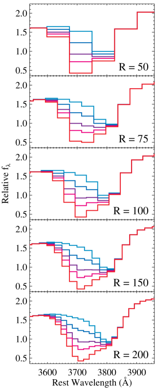
Figure 16: Artificial Ca H&K line profiles. The profiles are the same as shown in Figure 3. Different resolutions ($R=50$, 75, 100, 150, and 200) are shown in each panel from top to bottom.

However, we note that Si ii $\lambda 6355$ does not suffer these same problems, and $R=75$ should provide accurate (and reasonably precise) measurements of the ejecta velocity. For optical spectrographs, one can easily measure $v_{\rm Si\,II}$ to $z=0.3$. With red-sensitive CCDs and good sky subtraction one can use optical spectrographs to measure $v_{\rm Si\,II}$ to $z\approx 0.6$. With NIR spectrographs, one can easily measure $v_{\rm Si\,II}$ to $z\approx 2$ (neglecting the faintness of the SNe).

For the SED Machine, which aims to classify low-redshift SNe, it should also be able to measure $v_{\rm Si\,II}$. The proposed spectrograph on WFIRST would have a wavelength range of 0.6 – 2 $\mu$m, which should cover $v_{\rm Si\,II}$ to $z\approx 3$, well beyond the expected redshift range of WFIRST. Rodney et al. (2012) presented an HST observer-frame NIR spectrum of a $z=1.55$ SN Ia, SN Primo. The spectrum has a low S/N and is low-resolution ($R\approx 130$). But using the method of Blondin et al. (2006), we measure $v_{\rm Si~{}II}=-11200\pm 900$  km s^-1 at a phase of $6\pm 3$ d, corresponding to $v_{\rm Si~{}II}^{0}=-11700\pm 1000$  km s^-1. This corresponds, using the Foley et al. (2011) relations, to $(B_{\rm max}-V_{\rm max})_{0}=0.00\pm 0.07$ mag. The uncertainty in the velocity measurement is dominated by the low S/N of the spectrum, but the uncertainty in the intrinsic colour is still dominated by the uncertainty and scatter in the velocity-colour relation. None the less, SN Primo appears to be have a moderate intrinsic colour. This shows the potential of using velocity measurements for SN Ia cosmology even if the complexities of the Ca H&K profile prevents accurate measurements.

The additional knowledge of the Ca H&K profile provided here is a step toward further understanding of the full SED of SNe Ia. SNe Iax, which have compositions similar to that of SNe Ia, can be exceedingly useful for determining which specific atomic transitions contribute to SN Ia spectra. Because of their low ejecta velocities, SNe Iax may provide additional insight into the specific contributions from various lines for blended SN Ia features. Similarly, additional spectropolarimetric observations of SNe Ia, and particularly those that cover both Ca H&K and the Ca NIR triplet, NIR spectra, and good spectral sequences starting at early times should produce additional insight into the formation of a SN Ia SED.

Table 1: Derived Quantities for M12 Sample

SN	$z$	Eff. Phase	Stretch	M12 $v_{\rm Ca\,H\&K}$	Phase-corrected M12	Blue $v_{\rm Ca\,H\&K}$	Red $v_{\rm Ca\,H\&K}$	Ca/Si
		(d)		($10^{3}$  km s-1)	$v_{\rm Ca\,H\&K}$ ($10^{3}$  km s-1)	($10^{3}$  km s-1)	($10^{3}$  km s-1)	Ratio
PTF09dlc	0.0666	2.8	1.05 (0.03)	$-16.99$ (0.17)	$-17.78$ (0.67)	$-19.25$ (0.12)	$-10.47$ (0.19)	1.709 (0.050)
PTF09dnl	0.019	1.3	1.05 (0.02)	$-16.81$ (0.15)	$-17.17$ (0.33)	$-18.87$ (0.05)	$-9.71$ (0.07)	1.987 (0.047)
PTF09fox	0.0707	2.6	0.92 (0.04)	$-14.40$ (0.04)	$-15.14$ (0.62)	$-16.99$ (0.33)	$-10.28$ (0.31)	1.278 (0.041)
PTF09foz	0.05331	2.8	0.87 (0.06)	$-14.28$ (0.11)	$-15.07$ (0.67)	$-17.32$ (0.30)	$-10.02$ (0.28)	1.058 (0.006)
PTF10bjs	0.0303	1.9	1.08 (0.02)	$-16.47$ (0.22)	$-17.02$ (0.50)	$-21.68$ (0.10)	$-13.37$ (0.07)	0.790 (0.004)
PTF10hdv	0.0542	3.3	1.05 (0.07)	$-17.03$ (0.18)	$-17.94$ (0.78)	$-19.71$ (0.18)	$-10.94$ (0.22)	1.637 (0.048)
PTF10hmv	0.033	2.5	1.15 (0.01)	$-15.02$ (0.11)	$-15.72$ (0.59)	$-17.84$ (0.16)	$-9.92$ (0.18)	1.420 (0.026)
PTF10icb	0.0088	0.8	0.99 (0.03)	$-12.61$ (0.03)	$-12.85$ (0.20)	$-16.99$ (0.06)	$-10.25$ (0.05)	0.733 (0.004)
PTF10mwb	0.0312	$-0.4$	0.94 (0.03)	$-13.09$ (0.03)	$-12.99$ (0.09)	$-16.99$ (0.12)	$-10.24$ (0.12)	0.903 (0.008)
PTF10qjq	0.0288	3.5	0.96 (0.02)	$-11.87$ (0.08)	$-12.86$ (0.83)	$-17.64$ (0.24)	$-10.80$ (0.12)	0.459 (0.022)
PTF10tce	0.039716	3.5	1.07 (0.02)	$-16.02$ (0.05)	$-17.00$ (0.81)	$-19.81$ (0.17)	$-12.35$ (0.16)	0.850 (0.016)
PTF10wnm	0.0645	4.1	1.01 (0.03)	$-12.90$ (0.07)	$-14.04$ (0.96)	$-17.46$ (0.40)	$-10.66$ (0.24)	0.579 (0.034)
PTF10xyt	0.0484	3.2	1.07 (0.04)	$-15.01$ (0.08)	$-15.90$ (0.74)	$-18.74$ (0.48)	$-11.62$ (0.38)	0.810 (0.026)
SN2009le	0.01703	0.3	1.08 (0.01)	$-16.08$ (0.12)	$-16.16$ (0.14)	$-19.98$ (0.10)	$-12.24$ (0.10)	0.966 (0.001)

Table 2: SYNOW Model Parameters for SNe 2010ae and 2011fe

Parameter	O i	Na i	Mg ii	Si ii	S ii	Ca ii	HV Ca ii	Cr ii	Fe iii	Co ii
SN 2011fe
Si ii $\lambda 3858$
$\tau$	0.2	0.8	0.5	3	1.2	7	0	60	0.5	0.4
$v_{e}$	5	1	2	2	1.5	2.5		2	2.5	2
$T_{\rm exc}$	8	8	5	6	12	18		10	10	10
HV Ca
$\tau$	0.2	0	0.5	3	1.2	4	1.7	60	0.5	0.4
$v_{e}$	5		2	2	1.5	3.5	2	2	2.5	2
$T_{\rm exc}$	8		5	15	12	18	18	10	10	10
SN 2010ae
Si ii $\lambda 3858$
$\tau$	0.2	0.8	0.5	1	1.2	4	0	60	0.5	0.4
$v_{e}$	5	1	2	2	1.5	2.5		2	2.5	2
$T_{\rm exc}$	8	8	5	6	12	18		10	10	10
HV Ca
$\tau$	0.2	0	0.5	1.5	1.2	4	1	60	0.5	0.4
$v_{e}$	5		2	2	1.5	2	2	2	2.5	2
$T_{\rm exc}$	8		5	15	12	18	18	10	10	10

References

- Altavilla et al. (2007) Altavilla G. et al., 2007, A&A, 475, 585
- Ben-Ami et al. (2012) Ben-Ami S., Konidaris N., Quimby R., Davis J. T., Ngeow C. C., Ritter A., Rudy A., 2012, in Society of Photo-Optical Instrumentation Engineers (SPIE) Conference Series, Vol. 8446, Society of Photo-Optical Instrumentation Engineers (SPIE) Conference Series
- Blondin et al. (2006) Blondin S. et al., 2006, AJ, 131, 1648
- Blondin et al. (2012a) Blondin S., Dessart L., Hillier D. J., Khokhlov A. M., 2012a, ArXiv e-prints, 1211.5892
- Blondin et al. (2012b) Blondin S. et al., 2012b, AJ, 143, 126
- Bongard et al. (2008) Bongard S., Baron E., Smadja G., Branch D., Hauschildt P. H., 2008, ApJ, 687, 456
- Branch et al. (1985) Branch D., Doggett J. B., Nomoto K., Thielemann F.-K., 1985, ApJ, 294, 619
- Branch et al. (2005) Branch D., Baron E., Hall N., Melakayil M., Parrent J., 2005, PASP, 117, 545
- Branch et al. (2007) Branch D. et al., 2007, PASP, 119, 709
- Brown et al. (2012) Brown P. J. et al., 2012, ApJ, 753, 22
- Chomiuk et al. (2012) Chomiuk L. et al., 2012, ApJ, 750, 164
- Chornock & Filippenko (2008) Chornock R., Filippenko A. V., 2008, AJ, 136, 2227
- Conley et al. (2011) Conley A. et al., 2011, ApJS, 192, 1
- Fabricant et al. (1998) Fabricant D., Cheimets P., Caldwell N., Geary J., 1998, PASP, 110, 79
- Fisher et al. (1997) Fisher A., Branch D., Nugent P., Baron E., 1997, ApJ, 481, L89+
- Foley et al. (2009) Foley R. J. et al., 2009, AJ, 138, 376
- Foley et al. (2010) Foley R. J., Brown P. J., Rest A., Challis P. J., Kirshner R. P., Wood-Vasey W. M., 2010, ApJ, 708, L61
- Foley & Kasen (2011) Foley R. J., Kasen D., 2011, ApJ, 729, 55
- Foley et al. (2011) Foley R. J., Sanders N. E., Kirshner R. P., 2011, ApJ, 742, 89
- Foley (2012) Foley R. J., 2012, ApJ, 748, 127
- Foley et al. (2012a) Foley R. J. et al., 2012a, ArXiv e-prints, 1212.2209
- Foley et al. (2012b) Foley R. J. et al., 2012b, ApJ, 744, 38
- Foley et al. (2012c) Foley R. J. et al., 2012c, ApJ, 753, L5
- Foley et al. (2012d) Foley R. J. et al., 2012d, ApJ, 752, 101
- Garavini et al. (2004) Garavini G. et al., 2004, AJ, 128, 387
- Garavini et al. (2007) Garavini G. et al., 2007, A&A, 471, 527
- Gerardy et al. (2004) Gerardy C. L. et al., 2004, ApJ, 607, 391
- Green et al. (2012) Green J. et al., 2012, ArXiv e-prints, 1208.4012
- Hachinger et al. (2012) Hachinger S. et al., 2012, ArXiv e-prints, 1208.1267
- Hatano et al. (1999) Hatano K., Branch D., Fisher A., Baron E., Filippenko A. V., 1999, ApJ, 525, 881
- Höflich (1995) Höflich P., 1995, ApJ, 443, 89
- Höflich et al. (1998) Höflich P., Wheeler J. C., Thielemann F.-K., 1998, ApJ, 495, 617
- Hogg et al. (2010) Hogg D. W., Bovy J., Lang D., 2010, ArXiv e-prints, 1008.4686
- Horesh et al. (2012) Horesh A. et al., 2012, ApJ, 746, 21
- Kasen et al. (2003) Kasen D. et al., 2003, ApJ, 593, 788
- Kasen & Plewa (2007) Kasen D., Plewa T., 2007, ApJ, 662, 459
- Kelly (2007) Kelly B. C., 2007, ApJ, 665, 1489
- Kirshner et al. (1993) Kirshner R. P. et al., 1993, ApJ, 415, 589
- Lentz et al. (2000) Lentz E. J., Baron E., Branch D., Hauschildt P. H., Nugent P. E., 2000, ApJ, 530, 966
- Lentz et al. (2001) Lentz E. J., Baron E., Branch D., Hauschildt P. H., 2001, ApJ, 557, 266
- Li et al. (2001) Li W. et al., 2001, PASP, 113, 1178
- Maguire et al. (2012) Maguire K. et al., 2012, MNRAS, 426, 2359
- Margutti et al. (2012) Margutti R. et al., 2012, ApJ, 751, 134
- Matheson et al. (2008) Matheson T. et al., 2008, AJ, 135, 1598
- Matheson et al. (2012) Matheson T. et al., 2012, ApJ, 754, 19
- Mazzali et al. (2005a) Mazzali P. A. et al., 2005a, ApJ, 623, L37
- Mazzali et al. (2005b) Mazzali P. A., Benetti S., Stehle M., Branch D., Deng J., Maeda K., Nomoto K., Hamuy M., 2005b, MNRAS, 357, 200
- Nugent et al. (1995) Nugent P., Phillips M., Baron E., Branch D., Hauschildt P., 1995, ApJ, 455, L147
- Nugent et al. (1997) Nugent P., Baron E., Branch D., Fisher A., Hauschildt P. H., 1997, ApJ, 485, 812
- Nugent et al. (2011) Nugent P. E. et al., 2011, Nature, 480, 344
- Parrent et al. (2012) Parrent J. T. et al., 2012, ApJ, 752, L26
- Quimby et al. (2006) Quimby R., Höflich P., Kannappan S. J., Rykoff E., Rujopakarn W., Akerlof C. W., Gerardy C. L., Wheeler J. C., 2006, ApJ, 636, 400
- Rodney et al. (2012) Rodney S. A. et al., 2012, ApJ, 746, 5
- Röpke et al. (2012) Röpke F. K. et al., 2012, ApJ, 750, L19
- Shappee et al. (2013) Shappee B. J., Stanek K. Z., Pogge R. W., Garnavich P. M., 2013, ApJ, 762, L5
- Silverman et al. (2012) Silverman J. M., Ganeshalingam M., Li W., Filippenko A. V., 2012, MNRAS, 425, 1889
- Stanishev et al. (2007) Stanishev V. et al., 2007, A&A, 469, 645
- Suzuki et al. (2012) Suzuki N. et al., 2012, ApJ, 746, 85
- Tanaka et al. (2008) Tanaka M. et al., 2008, ApJ, 677, 448
- Tanaka et al. (2011) Tanaka M., Mazzali P. A., Stanishev V., Maurer I., Kerzendorf W. E., Nomoto K., 2011, MNRAS, 410, 1725
- Valenti et al. (2009) Valenti S. et al., 2009, Nature, 459, 674
- Wang et al. (2003) Wang L. et al., 2003, ApJ, 591, 1110
- Wang et al. (2009a) Wang X. et al., 2009a, ApJ, 699, L139
- Wang et al. (2009b) Wang X. et al., 2009b, ApJ, 697, 380
- Williams et al. (2010) Williams M. J., Bureau M., Cappellari M., 2010, MNRAS, 409, 1330
- Yaron & Gal-Yam (2012) Yaron O., Gal-Yam A., 2012, PASP, 124, 668