Echo State Queueing Network:
a new reservoir computing learning tool

Abstract

In the last decade, a new computational paradigm was introduced in the field of Machine Learning, under the name of Reservoir Computing (RC). RC models are neural networks which a recurrent part (the reservoir) that does not participate in the learning process, and the rest of the system where no recurrence (no neural circuit) occurs. This approach has grown rapidly due to its success in solving learning tasks and other computational applications. Some success was also observed with another recently proposed neural network designed using Queueing Theory, the Random Neural Network (RandNN). Both approaches have good properties and identified drawbacks.

In this paper, we propose a new RC model called Echo State Queueing Network (ESQN), where we use ideas coming from RandNNs for the design of the reservoir. ESQNs consist in ESNs where the reservoir has a new dynamics inspired by recurrent RandNNs. The paper positions ESQNs in the global Machine Learning area, and provides examples of their use and performances. We show on largely used benchmarks that ESQNs are very accurate tools, and we illustrate how they compare with standard ESNs.

Index Terms - Reservoir Computing, Echo State Network, Random Neural Network, Queueing Network, Machine Learning

I Introduction

Artificial Neural Networks (ANNs) are a class of computational models which have been proven to be very powerful as statistical learning tools to solve complicated engineering tasks as well as many theoretical issues. Several types of ANNs have been designed, some of them originating in the field of Machine Learning while others coming from biophysics and neuroscience. The Random Neural Network (RandNN) proposed by E. Gelenbe in 1989 [1], is a mathematical object inspired by biological neuronal behavior which merges features of Spiking Neural Networks and Queueing Networks. In the literature, actually two different interpretations of exactly the same mathematical model are proposed. One is a type of spiking neuron and the associated network which is called RandNNs. The other one is a new type of queue and networks of queues, respectively called G-queues and G-networks. The RandNN is a connectionist model where spikes circulate among the interconnected neurons. A discrete state-space is used to represent the internal state (potential) of each neuron. The firing times of the spikes are modeled as Poisson processes. The potential of each neuron is represented by a positive integer that increases when a spike arrives or decreases after the neuron fires. In order to use RandNNs in supervised learning problems, a gradient descent algorithm has been described in [2], and Quasi-Newton methods have been proposed in [3, 4]. Additionally, the function approximation properties of the model were studied in [5, 6]. The structure of the model leads to efficient numerical evaluation procedures, to good performance in learning algorithms and to easy hardware implementations. Consequently, since its introduction the model has been applied in a variety of scientific fields. Nevertheless, the RandNNs model suffers from limitations. Some of them are related to the use of a feedforward topology (see [7]). The original acronym to refer the model was RNN. In this work to avoid a conflict of notation, we use RandNN for Random Neural Networks, due to the use of RNNs in Machine Learning literature for Recurrent Neural Networks.

Concerning models with recurrences (circuits) in their topologies, they are recognized as powerful tools for a number of tasks in Machine Learning (both traditional ANNs and RandNNs). However, they have a main limitation which comes from the difficulty in implementing efficient training algorithms. The main drawbacks related to learning algorithms are the following: convergence is not always guaranteed, many algorithmic parameters are involved, sometimes long training times are required [8, 9]. For all those reasons learning using recurrent neural networks is principally feasible for relatively small networks.

Recently, a new paradigm called Reservoir Computing (RC) has been developed which overcome the main drawbacks of learning algorithms applied to networks with cyclic topologies. About ten years ago two main RC models were proposed: Echo State Networks (ESNs) [10] and Liquid State Machines (LSMs) [11]. Both models describe the possibility of using recurrent neural networks without adapting the weight connections involved in recurrences. The network outputs are generated using very simple learning methods such as classification or regression models. The RC approach have been successfully applied in many machine learning tasks achieving goods results, specially in temporal learning tasks [8, 11, 12].

In this paper we introduce a new type of RC method which uses some ideas from RandNNs. The paper is organized as follows: we begin by describing the RandNN model in Section II. In Section III, we introduce the two funding RC models. Section IV discusses the contribution of this paper, a new RC model similar to the ESN, but using also ideas inspired by queuing theory. Finally, we present some experimental results and we end with some conclusions as well as a discussion regarding future lines of research.

II Description of the
Random Neural Network Model

A Random Neural Network (RandNN) is a specific queuing network proposed in [1] which merges concepts from spiking neural networks and queuing theory. Depending on the context, its nodes are seen as queues or as spiking neurons. Each of these neurons receives spikes (pulses) from outside, which are of one out of two disjoint types, called excitatory (or positive) and inhibitory (or negative). Associated with a neuron there is an integer variable called the neuron’s potential. Each time a neuron receives an excitatory spike, its potential is increased by one. If a neuron receives an inhibitory spike and its potential was strictly positive, it decreases by one; if it was equal to $0$, it remains at that value. As far as the neuron’s potential is strictly positive, the neuron sends excitatory spikes to outside. When the neuron’s potential is strictly positive, we say that the neuron is excited or active. After numbering the neurons in an arbitrary order, let’s denote by $S_{u}(t)$ the potential of neuron $u$ at time $t$. During the periods when the neuron is active, it produces excitatory spikes with some rate $r_{u}>0$. In other words, the output process of the pulses coming out of an active neuron is a Poisson process. Then, a spike produced by neuron $u$ is transferred to the environment with probability $d_{u}$. For each synapse between neuron $u$ and $v$ an excitatory spike (respectively inhibitory spike) produced by $u$ is switched to neuron $v$ with probability $p^{+}_{v,u}$ (respectively $p^{-}_{v,u}$). In the literature related to RandNNs, the probability that a pulse generated at neuron $u$ goes to neuron $v$ is usually denoted by $p_{u,v}^{+/-}$. This is different from the notation used in the standard ANNs literature, where a direct connection between $u$ and $v$ is often denoted as $({v,u})$, that is, in the reverse order. In this paper we follow the latter notation. This routing procedure is performed independently of anything else happening in the network, including previous or future switches at the same neuron or at any other one. Observe that for any neuron $u$ we have

$$d_{u}+\sum_{v=1}^{N}p^{+}_{v,u}+\sum_{v=1}^{N}p^{-}_{v,u}=1,$$

where $N$ is the number of neurons in the network. The weight connection between any two neurons $u$ and $v$ ($u$ sending spikes to $v$) is defined as: $w^{+}_{v,u}=r_{u}p^{+}_{v,u}$ and $w^{-}_{v,u}=r_{u}p^{-}_{v,u}$.

Let us assume that the external (i.e. from the environment) arrival process of positive (respectively negative) spikes to neuron $u$ is Poisson with rate $\lambda^{+}_{u}$ (respectively with rate $\lambda^{-}_{u}$). Some of these rates can be 0, meaning that no spike of the considered type arrives at the given neuron coming from the network’s environment. In order to avoid the trivial case where nothing happens, we also must assume that $\sum_{u=1}^{N}\lambda^{+}_{u}>0$ (otherwise, the network is composed of neurons that are inactive at all times). Last, the usual independence assumptions between all the considered Poisson and routing processes in the model are assumed.

We call $\mathbf{S}(t)=(S_{1}(t),\cdots,S_{N}(t))$ the state of the network at time $t$. Observe that $\mathbf{S}$ is a continuous time Markov process over the state space $\mathbb{N}^{N}$. We will assume that $\mathbf{S}$ is irreducible and ergodic. We are interested in the network’s behavior in steady-state, so, let us assume that $\mathbf{S}$ is in equilibrium (that is, assume $\mathbf{S}$ is stationary). Let $\varrho_{u}$ be the probability (in equilibrium) that neuron $u$ is excited,

$$\varrho_{u}=\lim_{t\rightarrow\infty}\mathds{P}(S_{u}(t)>0).$$

This parameter is called the activity rate of neuron $u$. Since process $S$ is ergodic, for all neron $u$ we have $0<\varrho_{u}<1$. Gelenbe in [1, 13] shows that in an equilibrium situation the $\varrho_{u}$s satisfy the following non-linear system of equations:

$$\mbox{for each node\leavevmode\nobreak\ $u$, }\quad\varrho_{u}=\frac{T^{+}_{u}}{r_{u}+T^{-}_{u}},$$ (1)

$$\mbox{for each node\leavevmode\nobreak\ $u$, }\quad T^{+}_{u}=\lambda^{+}_{u}+\sum_{v=1}^{N}\varrho_{v}w^{+}_{u,v},$$ (2)

$$\mbox{for each node\leavevmode\nobreak\ $u$, }\quad T^{-}_{u}=\lambda^{-}_{u}+\sum_{v=1}^{N}\varrho_{v}w^{-}_{u,v},$$ (3)

with the supplementary condition that, for all neuron $u$, we have $\varrho_{u}<1$. In other words, under the assumption of irreducibility, if the system of equations (1), (2) and (3) has a solution $(\varrho_{1},\cdots,\varrho_{N})$ such that we have $\varrho_{u}<1$, for all neuron $u$, then the solution is unique and the Markov process is ergodic. Moreover, its stationary distribution is given by the product of the marginal probabilities of the neuron’s potential. For more details and proofs, see [1, 5].

As a learning tool used to learn some unknown function, we map the function’s variables to the external arrival rates, the $\lambda^{+}_{u}$s and $\lambda^{-}_{u}$s numbers (however, usually we set set $\lambda^{-}_{u}=0$ for all input neuron $u$, so we map the function’s variables to the $\lambda^{+}_{u}$s only). The network’s output is the set of loads. The learning parameters are the set of weights in the model. An appropriate optimization method (such as Gradient Descent) is used to find weights such that when the arrival rate (of positive spikes) equals the input data, the network output matches (with small error) the corresponding known output data values. The model has been widely used in fields such as: combinatorial optimization, machine learning problems, communication networks and computer systems [14, 15, 16, 17, 18].

III Reservoir computing methods

Recurrent Neural Networks are a large class of computational models used in several applications of Machine Learning and in neurosciences. The main characteristic of this type of ANNs is the existence of at least one feedback loop among the connections, that is, a circuit of connections.The cyclic topology causes that the non-linear transformation of the input history can be stored in internal states. Hence recurrent neural networks are a powerful tool for forecasting and time series processing applications. They are also very useful for building associative memories, in data compression and for static pattern classification [8]. However, in spite of these important abilities and of the fact that we have efficient algorithms for training neural networks without recurrences, no efficient algorithms exist for the case where recurrences are present.

Since the early 2000s, Reservoir Computing has gained prominence in the ANN community. In the two basic forms of the model described before, ESNs and LSMs, at least three well-differenced structures can be identified: the input layer, where neurons receive information from the environment; the reservoir (in ESNs) or liquid (in LSMs), a nonlinear “expansion” function implemented using a recurrent neuronal network; the readout, which is usually a linear function or a neural network without recurrences, producing the desired output.

The weight connections among neurons in the reservoir and the connections between input and reservoir neurons are fixed during the learning process, only the weights between input neurons and readout units, and between reservoir and readout units, are the object of the training process. The reservoir with its recurrences or circuits, allows a kind of “expansion” of the input and possibly of history data into a larger space. From this point of view, the reservoir idea is similar to the expansion function used in Kernel Methods, for example in the Support Vector Machine [19]. The projection can enhance the linear separability of the data [12]. On the other hand, the readout layer is built to be performant in learning, specially to be robust and fast in this process. The RC approach is based on the empirical observation that under certain assumptions, training only a linear readout is often sufficient to achieve good performance in many learning tasks [8]. For instance, the ESN model has the best known learning performance on the Mackey–Glass times series prediction task [20, 21].

The topology of a RC model consists of an input layer with $N_{\rm{a}}$ units sending pulses to the reservoir (and possibly also to the readout), a recurrent neural network with $N_{\rm{x}}$ units, where $N_{\rm{a}}\ll N_{\rm{x}}$, and a layer with $N_{\rm{b}}$ readout neurons having adjustable connections from the reservoir (and possibly from the input) layer(s).

The main difference between LSMs and ESNs consists in the type of nodes included in the reservoir. In the original LSM model the liquid was built using a model derived from Hodgkin-Huxley’s work, called Leaky Integrate and Fire (LFI) neurons. In the standard ESN model, the activation function of the units is most often $\tanh(\cdot)$. An ESN is basically a three-layered NN where only the hidden layer has recurrences, but allowing connections from input to readout (and, again, where learning is concentrated in the readout only). Our training data consists of $K$ pairs $(\mathbf{a}^{(k)},\mathbf{b}^{(k)})$, $k=1,\ldots,K$, of input-output values of some unknown function $f$, where $\mathbf{a}^{(k)}\in\mathds{R}^{N_{\rm{a}}}$, $\mathbf{b}^{(k)}\in\mathds{R}^{N_{\rm{b}}}$ and $\mathbf{b}^{(k)}=f(\mathbf{a}^{(k)})$. The weights matrices are $\mathbf{w}^{\rm{in}}$ (connections from input to reservoir), $\mathbf{w}^{\rm{r}}$ (connections inside the reservoir) and $\mathbf{w}^{\rm{out}}$ (connections between input or reservoir and readout), of dimensions $N_{\rm{x}}\times(1+N_{\rm{a}})$, $N_{\rm{x}}\times N_{\rm{x}}$ and $N_{\rm{b}}\times(1+N_{\rm{a}}+N_{\rm{x}})$, respectively. The first rows of $\mathbf{w}^{\rm{in}}$ and $\mathbf{w}^{\rm{out}}$ contain ones corresponding to the bias terms.

Each neuron $j$ of the reservoir has a real state $x_{j}$. When the input $\mathbf{a}$ arrives to the ESN, the reservoir first updates its state $\mathbf{x}=(x_{1},\ldots,x_{N_{x}})$ by executing

$${\mathbf{x}}:=\tanh\big{(}\mathbf{w}^{\rm{in}}[1;\mathbf{a}]+\mathbf{w}^{\rm{r}}\mathbf{x}\big{)},$$ (4)

and then, the ESN computes its outputs

$$\mathbf{y}:=\mathbf{w}^{\rm{out}}[1;\mathbf{a};\mathbf{x}],$$ (5)

where $[\cdot;\cdot]$ is the vertical vector concatenation.

If we think of the ESN has a dynamical system receiving a time series of inputs $\mathbf{a}(1),\mathbf{a}(2),\ldots$ and producing a series of outputs $\mathbf{y}(1),\mathbf{y}(2),\ldots$, the corresponding series of state values evolves according to

$$\mathbf{x}(t)=\tanh\big{(}\mathbf{w}^{\rm{in}}[1;\mathbf{a}(t)]+\mathbf{w}^{\rm{r}}\mathbf{x}(t-1)\big{)},$$

with the output at $t$ computed by $\mathbf{y}(t):=\mathbf{w}^{\rm{out}}[1;\mathbf{a}(t);\mathbf{x}(t)]$.

To ensure good properties in the reservoir, the $\mathbf{w}^{\rm{r}}$ matrix is usually scaled to control its spectral radius (to have $\rho(\mathbf{w}^{\rm{r}})<1$) [10]. The role of the spectral radius is more complex when the reservoir is built with spiking neurons (in the LSM model) [12, 22].

Several extensions of the two pioneering RC models have been suggested in the literature, such as: intrinsic plasticity [23], backpropagation-decorrelation [24], decoupled ESN [25], leaky integrator [26], Evolino [20], etc.

IV A new Reservoir Computing method:
Echo State Queuing Networks

In this paper, we propose to reach the objective of simultaneously keeping the good properties of the two models previously described. For this purpose, we introduce the Echo State Queuing Network (ESQN), a new RC model where the reservoir dynamics is based on a specific type of queuing network (RandNN) behavior in steady-state.

The architecture of an ESQN consists of an input layer, a reservoir and a readout layer. The input layer is composed of $N_{\rm{a}}$ random neural units which send spikes toward the reservoir or toward the readout nodes. The reservoir dynamics is designed inspired by the equations of recurrent RandNNs (see below). Let us index the input neurons from $1$ and $N_{\rm{a}}$, and the reservoir neurons from $N_{\rm{a}}+1$ to $N_{\rm{a}}+N_{\rm{x}}$.

When an input $\mathbf{a}$ is offered to the network, we first identify the rates of the external positive spikes with that input, that is: $\lambda^{+}_{u}=a_{u}$, and, as it is traditionally done in RandNNs, $\lambda^{-}_{u}=0$, for all $u=1,\ldots,N_{\rm{a}}$. In a standard RandNN, the neuron’s loads are computed solving the expressions (1), (2) and (3). More precisely, input neurons behave as a $M/M/1$ queues. The load or activity rate of neuron $u$, $u=1,\ldots,N_{a}$ is, in the stable case ($a_{u}<r_{u}$), simply $\varrho_{u}=a_{u}/r_{u}$. For reservoir units, the loads are computed solving the non-linear system composed of equations (1), (2) and (3). The network is stable if all obtained loads are $<1$.

In our ESQN model, we do the same for input neurons, but for the reservoir, we introduce the concept of state. The state is simply the vector of loads $\mathbf{\varrho}$. When we need the network output corresponding to a new input $\mathbf{a}$, we first compute a new state by using

$$\varrho_{u}:=\displaystyle{\frac{\displaystyle{\sum_{v=1}^{N_{\rm{a}}}\frac{a_{v}}{r_{v}}w^{+}_{u,v}+\sum_{v=N_{\rm{a}}+1}^{N_{\rm{a}}+N_{\rm{x}}}\varrho_{v}w^{+}_{u,v}}}{r_{u}+\displaystyle{\sum_{v=1}^{N_{\rm{a}}}\frac{a_{v}}{r_{v}}w^{-}_{u,v}+\sum_{v=N_{\rm{a}}+1}^{N_{\rm{a}}+N_{\rm{x}}}\varrho_{v}w^{-}_{u,v}}}},$$ (6)

for all $u\in[N_{\rm{a}}+1,N_{\rm{a}}+N_{\rm{x}}].$ When this is seen as a dynamical system, on the left we have the loads at $t$, and on the r.h.s. the loads at $t-1$.

The readout part is computed by a parametric function $g(\mathbf{w}^{\rm{out}},\mathbf{a},\mathbf{\varrho})$ (or $g(\mathbf{w}^{\rm{out}},\mathbf{a}(t),\mathbf{\varrho}(t))$ when this is used as a dynamical prediction system. In this paper we present the simple case of computing the readout using a linear regression. It is easy to change this by another type of function $g$, due to the independent structure between the reservoir and readout layers. Thus, the network output $\mathbf{y}(t)=[y_{1}(t),\ldots,y_{N_{\rm{b}}}(t)]$ is computed for any $m\in[1,N_{\rm{b}}]$ using expression (5) and it can be written as follows, where we use the temporal version at time $t$:

$$y_{m}(t)=\displaystyle{w_{m0}^{\text{out}}+\sum_{i=1}^{N_{\rm{a}}}w^{\text{out}}_{mi}a_{i}(t)}+\displaystyle{\sum_{i=1+N_{\rm{a}}}^{N_{\rm{a}}+N_{\rm{x}}}w^{\text{out}}_{mi}\varrho_{i}(t)}.$$ (7)

The output weights $\mathbf{w}^{\rm{out}}$ can be computed using some of the traditional algorithms to solve regressions such as the “ridge regression” or the least mean square algorithms [27].

V Experimental Results

In our numerical experiences, we consider a simulated time series data widely used in the ESN literature [10, 28] and two real world data sets about Internet traffic, used in research work about forecasting techniques [29, 30]. To evaluate the models’ accuracy, we use the Normalized Mean Square Error (NMSE):

$$\text{NMSE}=\displaystyle{\frac{\sum_{k=1}^{K}\sum_{j=1}^{N_{\rm{b}}}{\big{(}{b_{j}^{(k)}-y_{j}^{(k)}\big{)}^{2}}}}{\sum_{k=1}^{K}\sum_{j=1}^{N_{\rm{b}}}{\big{(}{b_{j}^{(k)}-\bar{b}_{j}\big{)}^{2}}}}},$$ (8)

where $\bar{b}_{j}$ is the empirical mean, and where we use the same notation as before for the data. The positive and negative weights of the ESQN model and the initial reservoir state were randomly initialized in the intervals $[0,0.2]$ and $[0,1]$, respectively. As usual, the training performance can depend on the choice of the starting weights. To take this into account, we experiment with $20$ different random initial weights and we calculate their average performance. The preprocessing data step consisted in rescaling the data in the interval $[0,1]$. The learning method used was offline ridge regression [31]. This algorithm contains a regularization parameter which is adjusted for each data set. The time series data considered were:

1. Fixed $10$th order nonlinear autoregressive moving average (NARMA) system. The series is generated by the following expression:
   $b(t+1)=0.3\,b(t)+0.05\,b(t){\sum_{i=0}^{9}b(t-i)}\\ +1.5\,s(t-9)\,s(t)+0.1,$ where $s(t)\sim\text{Unif}[0,0.5]$. We generated a training data with $1990$ samples and a validation set with $390$ samples.

2. Traffic data from an Internet Service Provider (ISP) working in $11$ European cities. The original data is in bits and was collected every $5$ minutes. We rescaled it in $[0,1]$. The size of the training data is $9848$ and the size of validation set is $4924$. The input neurons ($N_{\rm{a}}=7$) are mapped to the last $7$ points of the past data, that is with values from $t-6$ up to time $t$. This configuration was suggested in [29] where the authors discuss different neural network topologies taking into account seasonal traits of the data.

3. Traffic data from United Kingdom Education and Research Networking Association (UKERNA). The Internet traffic was collected every day. The network input at any time $t$ is the triple composed of the traffic at times $t$, $t-6$ and $t-7$, as studied in [29]. This small data set has $47$ training pairs and $15$ validation samples.

Table I: Comparison between ESN and ESQN. We give the NMSE obtained from $20$ independent trials, and the corresponding Confidence Interval (CI), for an ESN model and the proposed ESQN procedure. The reservoir size was $80$ units for the first data set and $40$ units for the other ones.

Series	Model	NMSE	CI
NARMA	ESN	$0.1401$	$\pm 0.0504$
	ESQN	$0.1004$	$\pm 0.0025$
ISP	ESN	$0.0062$	$\pm 9.8885\times 10^{-7}$
	ESQN	$0.0100$	$\pm 1.2436\times 10^{-4}$
UKERNA	ESN	$0.3781$	$\pm 0.0066$
	ESQN	$0.2030$	$\pm 0.0335$

The NARMA series data was studied in deep in [12, 21, 28, 32, 33]. For the last two data sets the performance using NN, ARIMA and Holt-Winters methods can be seen in [29]. A typical ESN model consists in a reservoir with the following characteristics: random topology, $N_{\rm{x}}$ large enough, sparsely connected (roughly between $15\%$ and $20\%$ of their weights are non-zeros) [8]. The specific ESN used has a sparsity of $15\%$ and spectral radius of $0.95$ in its reservoir matrix. In [12], the authors obtained the best performance in the NARMA data problem when the spectral radius was close to $1$.

The ESN performance can be improved using leaky-integrator neurons [26], feedback connections [8] or initializing the reservoir weights using another initializing criteria [33, 34]. Both models have $80$ units in the reservoir for the NARMA data and $40$ units for the other two data sets. In this paper, in order to compare the performance of the ESQN and ESN models we use the standard versions of each of them.

Table I presents the accuracy of the ESQN and ESN models. In the last column we give a $95\%$ confidence interval obtained from $20$ independent runs. We can see that for the $10$th order NARMA and UKERNA data the performance obtained with ESQN is better than with ESN (even if in the NARMA case, the confidence intervals have a “slight” non-empty intersection). In the case of the European ISP data, ESN shows a significant better performance. Observe that in all cases the accuracy obtained with ESQN was very good. Also observe that we are using some years of cumulated knowledge about ESNs in our implementation, which we are comparing with our first versions of our new largely unexplored ESQN model.

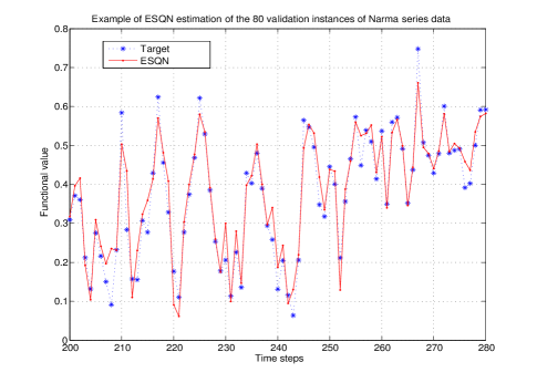
Figure 1: Example of ESQN prediction for $80$ time steps of fixed $10$th NARMA validation data set. The reservoir was randomly initialized and it had $80$ units.

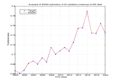
Figure 2: Example of ESQN prediction for $20$ instances in the validation set of the European ISP traffic data. The instances correspond to time steps between $4900$ and $4920$. The reservoir was randomly initialized and it had $40$ neurons.

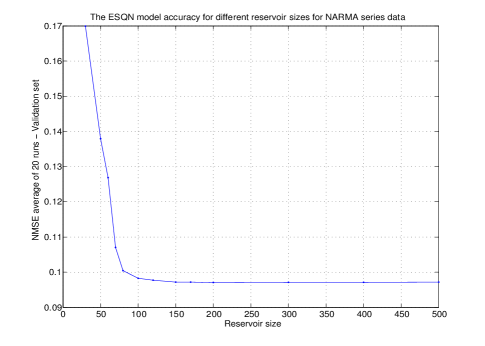
Figure 3: The ESQN model performance for different reservoir sizes which are computed for $10$th NARMA validation data set. The reservoir weights were randomly initialized. Figure shows the NMSE average achieved in $20$ runs with different ESQN initial weights.

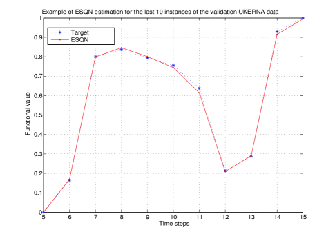
Figure 4: ESQN estimation for UKERNA validation data set. The reservoir weights were randomly initialized. The reservoir size is $40$.

Figure 3 shows that the reservoir size is an important parameter affecting the performance of the ESQN. This also happens with the ESN model: in general, a larger reservoir enriches the learning abilities of the model. The sparsity and density of the reservoir in the ESQN model was not studied in this work. It is left for future efforts. NARMA is an interesting time series data where the outputs depend on both the input and previous outputs. The modeling problem is difficult to solve due to the non-linearity of the data and the necessity of having some kind of long memory. Figure 1 illustrates an estimation of ESQN with $80$ units in the reservoir which are randomly chosen in $[0,0.2]$. Figures 2 and 4 show the prediction values for an interval of validation data. Figure 2 shows the prediction of $20$ instances beginning at time $4900$ of the validation set. The main difficulty to model UKERNA data (using day scale) is that the training set is small. In spite of this, Figure 4 illustrates the good performance of the ESQN model. This figure shows the estimation of the last $10$ instances in the validation data.

VI Conclusions

In this contribution, we have presented a new type of Reservoir Computing model which we call Echo State Queuing Network (ESQN). It combines ideas from queueing and neural networks. It is based on two computational models: the Echo State Network (ESN) and the Random Neural Network. Both methods have been successfully used in forecasting and machine learning problems. Particularly, ESNs have been applied in many temporal learning tasks. Our model was used to predict three time series data which are widely used in the machine learning literature. In all cases tested, the performance results have been very good. We empirically investigated the relation between the reservoir size and the ESQN performance. We found that the reservoir size has a significant impact on the accuracy. Another positive property of ESQNs is their simplicity, since reservoir units are just counter functions. Last, our tool is very easy to implement, both in software and in hardware.

There are still several aspects of the model to be studied in future work. Some examples are the impact of the sparsity of the reservoir weights, the weight initialization methods used, the scaling of reservoir weights and the utilization of leaky integrators.

References

- [1] E. Gelenbe, “Random Neural Networks with Negative and Positive Signals and Product Form Solution,” Neural Computation, vol. 1, no. 4, pp. 502–510, 1989.
- [2] ——, “Learning in the recurrent random neural network,” Neural Computation, vol. 5, pp. 154–164, 1993.
- [3] A. Likas and A. Stafylopatis, “Training the Random Neural Network using Quasi-Newton Methods,” Eur.J.Oper.Res, vol. 126, pp. 331–339, 2000.
- [4] S. Basterrech, S. Mohammed, G. Rubino, and M. Soliman, “Levenberg-Marquardt Training Algorithms for Random Neural Networks,” Computer Journal, vol. 54, no. 1, pp. 125–135, January 2011. [Online]. Available: http://dx.doi.org/10.1093/comjnl/bxp101
- [5] E. Gelenbe, “The Spiked Random Neural Network: Nonlinearity, Learning and Approximation,” in Proc. Fifth IEEE International Workshop on Cellular Neural Networks and Their Applications, London, England, april 1998, pp. 14–19.
- [6] E. Gelenbe, Z. Mao, and Y. Da-Li, “Function Approximation by Random Neural Networks with a Bounded Number of Layers,” Journal of Differential Equations and Dynamical Systems, vol. 12, pp. 143–170, 2004.
- [7] M. Georgiopoulos, C. Li, and T. Koçak, “Learning in the feed-forward random neural network: A critical review,” Performance Evaluation, vol. 68, no. 4, pp. 361 – 384, 2011. [Online]. Available: http://www.sciencedirect.com/science/article/pii/S0166531610000970
- [8] M. Lukos̆evic̆ius and H. Jaeger, “Reservoir computing approaches to recurrent neural network training,” Computer Science Review, pp. 127–149, 2009. [Online]. Available: http://dx.doi.org/10.1016/j.cosrev2009.03.005
- [9] K. Doya, “Bifurcations in the learning of Recurrent Neural Networks,” in IEEE International Symposium on Circuits and Systems, 1992, pp. 2777–2780.
- [10] H. Jaeger, “The “echo state” approach to analysing and training recurrent neural networks,” German National Research Center for Information Technology, Tech. Rep. 148, 2001.
- [11] W. Maass, T. Natschläger, and H. Markram, “Real-time computing without stable states: a new framework for a neural computation based on perturbations,” Neural Computation, pp. 2531–2560, november 2002.
- [12] D. Verstraeten, B. Schrauwen, M. D’Haene, and D. Stroobandt, “An experimental unification of reservoir computing methods,” Neural Networks, no. 3, pp. 287–289, 2007.
- [13] E. Gelenbe, “Product-Form Queueing Networks with Negative and Positive Customers,” Journal of Applied Probability, vol. 28, no. 3, pp. 656–663, September 1991.
- [14] E. Gelenbe, Z. Xu, and E. Seref, “Cognitive Packet Networks,” in 11th IEEE International Conference on Tools with Artificial Intelligence (ICTAI’99), 1999, pp. 47–54.
- [15] G. Sakellari, “The Cognitive Packet Network: A Survey,” The Computer Journal, vol. 53, no. 3, pp. 268–279, 2010. [Online]. Available: http://comjnl.oxfordjournals.org/cgi/content/abstract/bxp053v1
- [16] G. Rubino, “Quantifying the Quality of Audio and Video Transmissions over the Internet: the PSQA Approach,” in Design and Operations of Communication Networks: A Review of Wired and Wireless Modelling and Management Challenges, ser. Edited by J. Barria. Imperial College Press, 2005.
- [17] E. Gelenbe and F. Batty, “Minimum cost graph covering with the random neural network,” in Computer Science and Operations Research. New York: Pergamon, 1992, pp. 139–147.
- [18] H. Cancela, F. Robledo, and G. Rubino, “A GRASP algorithm with RNN based local search for designing a WAN access network,” Electronic Notes in Discrete Mathematics, vol. 18, pp. 59–65, 2004. [Online]. Available: http://dx.doi.org/10.1016/j.endm.2004.06.010
- [19] C. Cortes and V. Vapnik, “Support-Vector Networks,” Mach. Learn., vol. 20, no. 3, pp. 273–297, Sep. 1995. [Online]. Available: http://dx.doi.org/10.1023/A:1022627411411
- [20] J. Schmidhuber, D. Wierstra, M. Gagliolo, and F. Gomez, “Training Recurrent Networks by Evolino,” Neural Computation, vol. 19, no. 3, pp. 757–779, Mar. 2007. [Online]. Available: http://dx.doi.org/10.1162/neco.2007.19.3.757
- [21] H. Jaeger and H. Haas, “Harnessing nonlinearity: Predicting chaotic systems and saving energy in wireless communication,” Science, vol. 304, no. 5667, pp. 78–80, 2004. [Online]. Available: http://www.sciencemag.org/content/304/5667/78.abstract
- [22] H. Paugam-Moisy and S. M. Bohte, Handbook of Natural Computing. Springer-Verlag, Sep. 2009, ch. Computing with Spiking Neuron Networks. [Online]. Available: http://liris.cnrs.fr/publis/?id=4305
- [23] B. Schrauwen, M. Wardermann, D. Verstraeten, J. J. Steil, and D. Stroobandt, “Improving reservoirs using Intrinsic Plasticity,” Neurocomputing, vol. 71, pp. 1159–1171, March 2007.
- [24] J. J. Steil, “Backpropagation-Decorrelation: online recurrent learning with O(n) complexity,” In Proceedings of IJCNN’04, vol. 1, 2004.
- [25] Y. Xue, L. Yang, and S. Haykin, “Decoupled Echo State Networks with lateral inhibition,” Neural Networks, no. 3, pp. 365–376, 2007.
- [26] H. Jaeger, M. Lukos̆evic̆ius, D. Popovici, and U. Siewert, “Optimization and applications of Echo State Networks with leaky-integrator neurons,” Neural Networks, no. 3, pp. 335–352, 2007.
- [27] W. Press, S. Teukolsky, W. Vetterling, and B. Flannery, Numerical Recipes in C, 2nd ed. Cambridge, UK: Cambridge University Press, 1992.
- [28] A. Rodan and P. Tin̆o, “Minimum Complexity Echo State Network,” IEEE Transactions on Neural Networks, pp. 131–144, 2011. [Online]. Available: http://dx.doi.org/10.1109/TNN.2010.2089641
- [29] P. Cortez, M. Rio, M. Rocha, and P. Sousa, “Multiscale Internet traffic forecasting using neural networks and time series methods,” Expert Systems, 2012. [Online]. Available: http://dx.doi.org/10.1111/j.1468-0394.2010.00568.x
- [30] R. Hyndman, “Time Series Data Library,” Accessed on: August 31, 2012. [Online]. Available: http://robjhyndman.com/TSDL/miscellaneous/
- [31] M. Lukos̆evic̆ius, H. Jaeger, and B. Schrauwen, “Reservoir Computing Trends,” KI - Künstliche Intelligenz, pp. 1–7, 2012. [Online]. Available: http://dx.doi.org/10.1007/s13218-012-0204-5
- [32] A. F. Atiya and A. G. Parlos, “New results on recurrent network training: unifying the algorithms and accelerating convergence,” IEEE Trans. Neural Networks, vol. 11, pp. 697–709, 2000.
- [33] S. Basterrech, C. Fyfe, and G. Rubino, “Self-Organizing Maps and Scale-Invariant Maps in Echo State Networks,” in Intelligent Systems Design and Applications (ISDA), 2011 11th International Conference on, nov. 2011, pp. 94 –99.
- [34] M. Lukos̆evic̆ius, “On self-organizing reservoirs and their hierarchies,” Jacobs University, Bremen, Tech. Rep. 25, 2010.