Modeling collective human mobility: Understanding exponential law of intra-urban movement

Abstract

It is very important to understand urban mobility patterns because most trips are concentrated in urban areas. In the paper, a new model is proposed to model collective human mobility in urban areas. The model can be applied to predict individual flows not only in intra-city but also in countries or a larger range. Based on the model, it can be concluded that the exponential law of distance distribution is attributed to decreasing exponentially of average density of human travel demands. Since the distribution of human travel demands only depends on urban planning, population distribution, regional functions and so on, it illustrates that these inherent properties of cities are impetus to drive collective human movements.

Understanding human movement patterns is considered as a long-term challenging work for a long time. It is very crucial to urban planning Rozenfeld2008b ; Jing2012 ; Zheng2011 , epidemics spreading Balcan22122009 ; Colizza2007 ; Wang2012 and traffic engineering Viboud21042006 ; Jung2012 ; Goh2012 . During the past few years, various mobile devices (e.g. cellphones and GPS navigators) that support geolocation have been widely used in our daily life. As proxies, these devices record massive amounts of individual tracks. Benefited from it, the research of human mobility has attracted more and more attention of scientists from multiple disciplines such as physics, computer science and biology.

In recent studies, Brockmann et al. Brockmann2006 discovered human travel displacements can be described by a power-law distribution by investigating the dispersal of bank notes in the United States. González et al. Gonzalez2008 studied mobility patterns of mobile phone users in European countries and found that their travel distances are distributed according to a truncated power-law. Moreover, the similar scaling law was also observed in Song2010a and Jiang2009 separately. Therefore, in order to understand the cause of the scaling law, some researchers tried to propose possible explanations from individual movement viewpoint Han2011 ; Hu2011a . It is worthy to note that these researches characterized human travel occurred in large scale of space, including trips from countries to countries or cities to cities.

Furthermore, there are also many studies which focus on human movement in urban areas. For example, trajectories of passengers by taxis were investigated separately in three cities: Lisbon Veloso2011 , Beijing Liang2012 and Shanghai Peng2012 . And the three studies all suggested that trip distances obey exponential distributions rather than power-law ones. Bazzani et al. Bazzani2010 analyzed daily round-trip lengths of private cars’ drivers in Florence and revealed an exponential law of lengths too. In addition, the distances of individuals’ movement in the London subway were found obviously deviating from the power-law distribution as well Roth2011 . A more convincing evidence is that exponential distributions of intra-urban travel distances were demonstrated respectively in eight cities of Northeast China by analyzing the mobile phone data Kang2012 , which was not restricted to means of transportation. Even though a lot of empirical studies, the understanding of intra-urban mobility is still limited and there are no reasonable model to account for the exponential law to the best of our knowledge.

In order to understand the exponential law of collective human mobility in urban areas, it is essential to model individual flows from one region to the other in a city. As we know, the gravity model Barthelemy2010 has already been applied widely to predict flows, including human travel Balcan22122009 ; Jung2012 , cargo ship movement Kaluza06072010 and telephone communications Krings2009 . Assuming $T_{ij}$ is the flux of individual between location $i$ (with population $P_{i}$) and location $j$ (with population $P_{j}$) and $d_{ij}$ is the distance between the two locations, a general gravity law Simini2012a can be represented by

$$T_{ij}=K\frac{P_{i}^{\alpha}P_{j}^{\beta}}{f(d_{ij})}$$ (1)

where $K$, $\alpha$ and $\beta$ are tunable parameters and $f(d_{ij})$ is often selected as a power or exponential function of $d_{ij}$. Especially, the gravity model with $\alpha=\beta=1$ can be derived from entropy maximization Wilson-67 . Despite the prevailing gravity model, it still has some disadvantages Simini2012a . Particularly, the gravity model is incompetent to explain the discrepancy of the numbers of individual flows in both directions between a pair of locations. Consequently, Simini et al. Simini2012a put forward the radiation model without parameters:

$$\langle T_{ij}\rangle=T_{i}\frac{P_{i}P_{j}}{(P_{i}+P_{ij})(P_{i}+P_{j}+P_{ij})}$$ (2)

where $\langle T_{ij}\rangle$ is the expected flux from $i$ to $j$, $T_{i}$ is the number of trips started from $i$ and $P_{ij}$ is total population of locations (except $i$ and $j$) from which to $i$ the distance is less than or equal to $d_{ij}$. The model can predict population movement between cities or countries successfully, but it is not clear whether the model applies to intra-urban movement as well.

Therefore, by exploring human travels by taxis in Beijing, it is aimed to figure out the answers to the following questions in the paper:

• Whether can the radiation model predict intra-urban human flows? If not, how to model human mobility in urban areas.

• What is the origin of the exponential law in intra-urban human mobility? Why do the distributions of travel distances in urban areas disagree with the ones at a larger scale? What is the inherent impetus to drive collective human movement?

I Empirical analysis of taxis’ GPS data

I.1 Data description

Here, we use the taxis’ GPS data generated by over 10000 taxis in Beijing, China, during three months ended on Dec. 31st, 2010 Liang2012 . From taxis’ locations and statuses of occupation (with passengers or without passengers), trajectories of passengers can be observed. In order to study intra-urban human mobility patterns, a total of 12009383 individuals’ tracks were collected which occurred inside the 6th Ring Road of Beijing.

For the purpose of investigating individual flows between regions in urban areas, the urban area in a map can be divided into discrete grid-like cells of size $s\times s$ (selection of $s$ will be described below). The number of cells is $N$ and the Euclidean distance between the centers of cell $i$ and $j$ is defined as $d_{ij}$. Therefore, pick-up points (origins) and drop-off points (destinations) of trajectories can be simplified to cells which they lie in. As illustrated in Fig. 1, an individual trip can be represented by a tuple $(l_{O},l_{D},t_{O},t_{D})$, where $l_{O}$ and $l_{D}$ are the origin and destination cells ($l_{O},l_{D}\in\{1,2,\ldots,N\}$), $t_{O}$ and $t_{D}$ are the departure and arrival times.

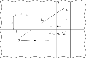
Figure 1: Illustration of the grid division on a map. The cell size is $s\times s$. The solid line shows an individual trajectory from cell $i$ to $j$, which can be denoted by the tuple $(i,j,t_{O},t_{D})$. And the distance $d_{ij}$ between cell $i$ and $j$ is described by the dashed line.

I.2 Choice of cell size

After dividing the urban areas into lattices, a trip length can be approximated by the distance between centers of cells which the pick-up and drop-off points lie in. In fact, it can be imagined that the location errors will become more and more large with increasing the cell size. At the same time, too small cell size is also undesirable because it would not reflect the regular mobility patterns between different regions obviously and increase computing costs. Therefore, it is important to choose an appropriate cell size to model urban mobility better. As shown in Fig. 2a, when cell size is larger than 0.01 degree, there is some deviation from the real distribution of trip displacements. So the cell size $s$ is determined as 0.01 degree in the following paper.

For the cell size $s$ is $0.01^{\circ}$, the probability distribution of approximated distances is plotted in Fig. 2b. Bescause the fraction of trips whose distances are less than 20km can reach nearly 98%, the curve can be fitted very well by an exponential function $y=Ce^{-\lambda x}$ with parameter $\lambda=0.230$.

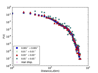
(a)

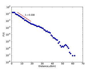
(b)

Figure 2: Distributions of trip distances. (a) The comparison of distributions between approximated distances in different cell sizes and actual distances. (b) The distribution of approximated distances when cell size $s$ is $0.01^{\circ}$.

I.3 Geographic distributions of origins and destinations

Considering pick-up and drop-off points of human trajectories respectively, the probability density distributions of them for three different months are obtained by Gaussian kernel density estimation (GKDE) method, which are visualized in Fig. 3. From the figure, it can be seen that density maps of origins/destinations for the three months have similar hot spots and these hot spots, such as Zhongguancun, Xidan, Beijing West Railway Station and so on, accord with our intuition very well.

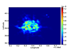
(a) 2010.10 (Origins)

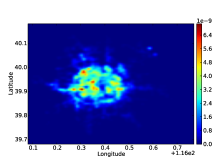
(b) 2010.11 (Origins)

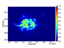
(c) 2010.12 (Origins)

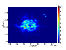
(d) 2010.10 (Destinations)

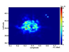
(e) 2010.11 (Destinations)

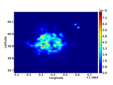
(f) 2010.12 (Destinations)

Figure 3: Gaussian kernel density estimations of origins and destinations for three months.

In order to quantify the similarities among geographic distributions of origins and destinations for the three months, we assign the probability for each cell as the fraction of origins/destinations falling into the grid cell. Actually, the probability distribution defined reflect spatial distribution patterns of human traveling intensity directly. After calculating the discrete probability distributions of origins/destinations for the three months, the similarity between distributions can be measured by a cosine value. To be specific, assuming two discrete probability distributions $\{p_{i}\}$ and $\{q_{i}\}$ ($i=1,\ldots,N$), the similarity $Sim_{cos}$ between them is defined by

$$Sim_{cos}=\frac{\sum_{i=1}^{N}{p_{i}q_{i}}}{\sqrt{\sum_{i=1}^{N}{p_{i}^{2}}}\sqrt{\sum_{i=1}^{N}{q_{i}^{2}}}}.$$

So, the similarity is assigned to a value between 0 and 1. The nearer the value approaches one, the more similar the two distributions are. The similarities between all distributions of origins/destinations for the three months are shown in Table 1. It is noticed that most values of similarity are larger than 0.95, which indicates that distributions, whether between origins and destinations or between different months, all resemble each other and follow similar patterns. In addition, it demonstrates that collective travel behaviors in different regions of urban areas are stable over time.

Table 1: The cosine similarities among distributions of origins/destinations for three months

	201010(O)	201011(O)	201012(O)	201010(D)	201011(D)	201012(D)
201010(O)	1.0	0.996	0.995	0.951	0.957	0.961
201011(O)	0.996	1.0	0.999	0.945	0.958	0.963
201012(O)	0.995	0.999	1.0	0.943	0.956	0.963
201010(D)	0.951	0.945	0.943	1.0	0.996	0.994
201011(D)	0.957	0.958	0.956	0.996	1.0	0.999
201012(D)	0.961	0.963	0.963	0.994	0.999	1.0

But it must be noted that geographic distributions of origins/destinations considered here are only based on human travels by taxis. It is not clear whether there is obvious bias with all intra-urban movement by different kinds of transport, including private cars, buses, subways, and taxis. Thus, the geo-tagged Sina Weibo data during 4 weeks in 2012 are collected for comparison (The data description is given in appendix A). From the geographic locations of posts, movements of Weibo users in Beijing are observed. Like the dataset of taxis, it also can characterize human trails in different geographic regions, but is independent of means of transportation. Then the geographic distributions of passengers’ destinations and geo-tagged microblogs’ locations are compared, which is illustrated in Fig. 4. From the graph, it can be seen that hot spots reflected by the two datasets are similar especially within the Fourth Ring Road of the city. The main difference between them is that the spectrum of human travel in Sina Weibo dataset is larger than one in taxis dataset. It is mainly because the urban planning of Beijing has been extending outward for the two years. And the cosine similarity between these two distributions is 0.829, which is high and validates our impressions further. Because of the similar distribution patterns of destinations and microblogs’ locations described by the two different datasets, it can be conjectured that means of transportation has only a very small impact on the geographic distribution of origins/destinations of human travel in urban areas.

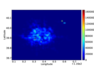
(a) Taxis(2010.10.1–2010.12.31)

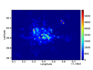
(b) Sina Weibo(2012.10.8–2012.11.4)

Figure 4: The geographic distributions for the two datasets.

Note that some studies are able to infer land use and regional functions successfully through analyzing spatiotemporal variation of human movement captured from passengers by taxis Zheng2011 or cellphone users Toole2012 . In fact, because geographic distribution of origins/destinations is influenced by demands for mobility, these all demonstrate that the distribution patterns of traveling demands or intensity are mainly related to inherent properties of the city, such as urban planning, regional functions, population density and so on, rather than means of transport.

II Modeling intra-urban human mobility

In the section, it is aimed to explore urban flows using tracks of passengers by taxis. Because the urban area has been divided into grid cells, we try to model and predict traffic flows between these grid cells.

II.1 Radiation model

Recently, the radiation model Simini2012a , which is parameter-free and only requires information of population distribution, was proposed to characterize mobility patterns between cities or countries. It overcomes some shortcomings of the gravity model and predicts traffic flows more precisely. So it is wished to verify whether the radiation model can be utilized to simulate collective human travel in urban areas of the city. But in urban areas, it is difficult to obtain population distribution directly because of high mobility of people. Instead we use the distribution of destinations in the simulation. It is more reasonable because the number of destinations in a grid cell describes human travel intensity in the region.

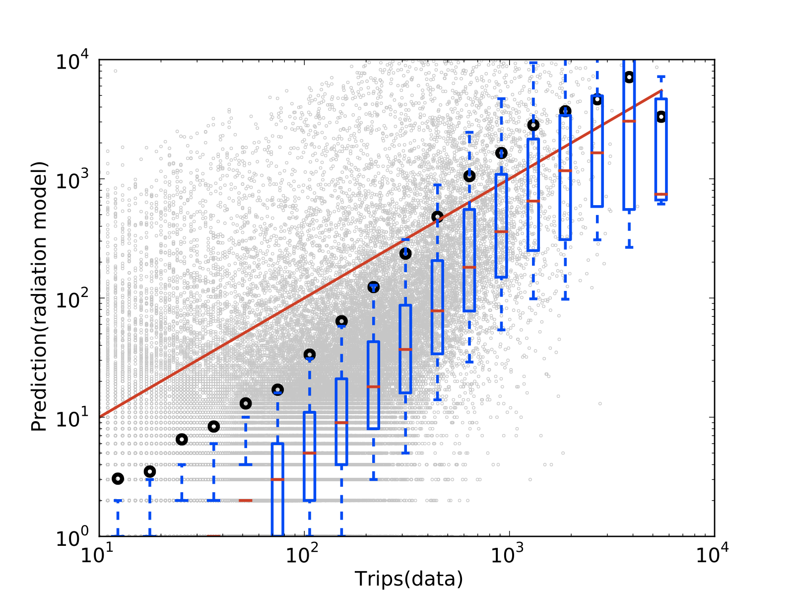
(a) Prediction(radiation model)

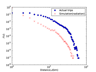
(b) Probability Distribution of trip length

Figure 5: Simulation by the radiation model. (a) Prediction of traffic flows between grid cells. Grey points stand for the relationship between actual and predicted flux of each pair of grid cells. The red line $y=x$ stands for the actual values equal with predicted values. The black circles denote mean values of prediction in the bins. The ends of whisker represent the 9th and 91st percentile in the bin. (b) Probability distributions of actual and predicted trip length.

The results of simulation by the radiation model is shown in Fig. 5. From the figure, it seems that the predicted flux has a large deviation from the actual ones and the model underestimates the probability of trips with distances larger than 1km. There are two possible reasons: one is that the destinations distribution may have some bias with actual population distribution; the other is that, unlike trips between countries or cities, the population distribution may be only one of factors to influence human movement because people often move frequently for various purposes in urban areas. Therefore, it is necessary to consider a new model to understand intra-urban human mobility patterns.

II.2 Our model

As for trips occurred during a period of time, it can be calculated that how many of them had left from or arrived at each cell. So the probability that people leave from/arrive at each cell is defined as follows

$$P_{O}(i) = \frac{\#\text{ of trips leaving from the cell }i}{\#\text{ of trips}},$$

$$P_{D}(i) = \frac{\#\text{ of trips arriving at the cell }i}{\#\text{ of trips}},i=\{1,2,\ldots,N\}.$$

Actually, $P_{O}$ and $P_{D}$ correspond to the distributions of origins and destinations separately. As demonstrated in subsection I.3, it must be noted that $P_{O}$ and $P_{D}$ only depend on population distribution, urban planning (land-use and transportation planning) and other environmental factors. The cells having large $P_{O}$ or $P_{D}$ often lie in prosperous commercial/entertainment regions, developed residential areas, transport hubs and so on.

Intuitively, the probability of a trip’s occurrence has positive correlations with $P_{O}$ of origin cell and $P_{D}$ of destination cell, but has a negative correlation with the Euclidean distance between the two cells. Hence, in our model the probability of a trip reaching cell $j$, conditioned on starting from cell $i$, is defined as follows

$$P(j|i)\propto\frac{P_{D}(j)}{f(d_{ij})}$$

where $f(d)$ is a function of distance between cells. In the paper, two frequently used forms of $f(d)$ are given by

$$Power-law : f(d)=d^{\sigma}$$

$$Exponential : f(d)=e^{\lambda d}$$

where $\sigma$ and $\lambda$ are parameters whose values rely on the specific system and reflect the effect of distance on human travel. So the happening probability of a trip from cell $i$ to $j$ can be derived as

$$P(i\to j) = P_{O}(i)P(j|i)$$ (3)

$$= P_{O}(i)\frac{P_{D}(j)/f(d_{ij})}{\sum_{k\neq i}{P_{D}(k)/f(d_{ik})}}.$$

And the expected number of trips from cell $i$ to $j$ can be obtained

$$\langle T_{ij}\rangle = TP(i\to j)$$ (4)

$$= \frac{T}{\sum_{k\neq i}{P_{D}(k)/f(d_{ik})}}\frac{P_{O}(i)P_{D}(j)}{f(d_{ij})}$$

$$= \frac{T}{M(i)}\frac{P_{O}(i)P_{D}(j)}{f(d_{ij})}.$$

where $M(i)=\sum_{k\neq i}{P_{D}(k)/f(d_{ik})}$ and $T$ is the total number of trips.

Note that it can be concluded that $P_{O}\approx P_{D}$ because the cosine similarity between distributions of origins and destinations is greater than 0.95 in taxis dataset. Furthermore, when considering human travel during a long time, it is reasonable to assume $P_{O}=P_{D}$ due to round-trip patterns in urban areas. As described in the gravity model, the number of trips from cell $i$ to $j$ is equal with the one from cell $j$ to $i$. However, that is not the case in our model because the values of $M(i)$ and $M(j)$ depend on locations of $i$ and $j$ respectively, which are often not equal to each other. Therefore, it is more consistent with our intuition.

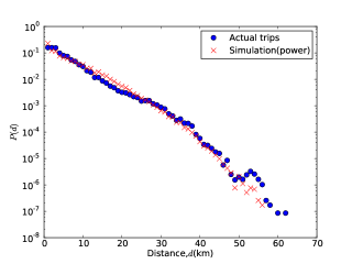
(a) Simulation by our model (power-law)

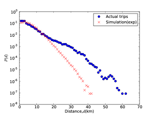
(b) Simulation by our model (exponential)

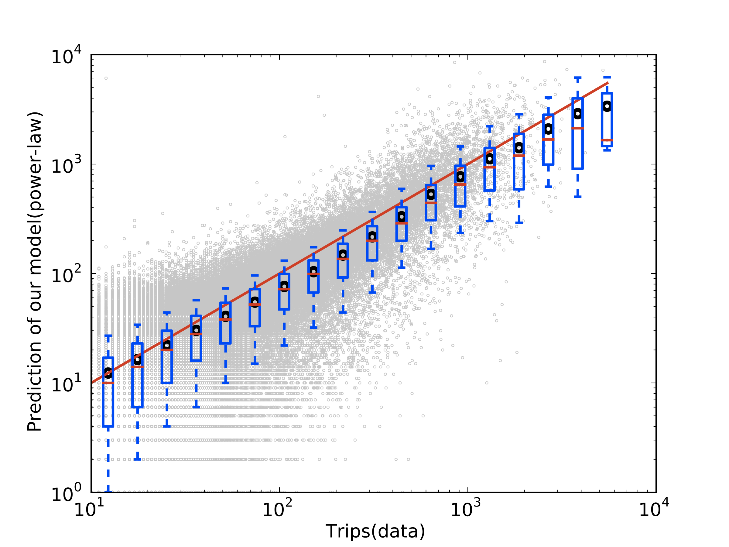
(c) Prediction by our model (power-law)

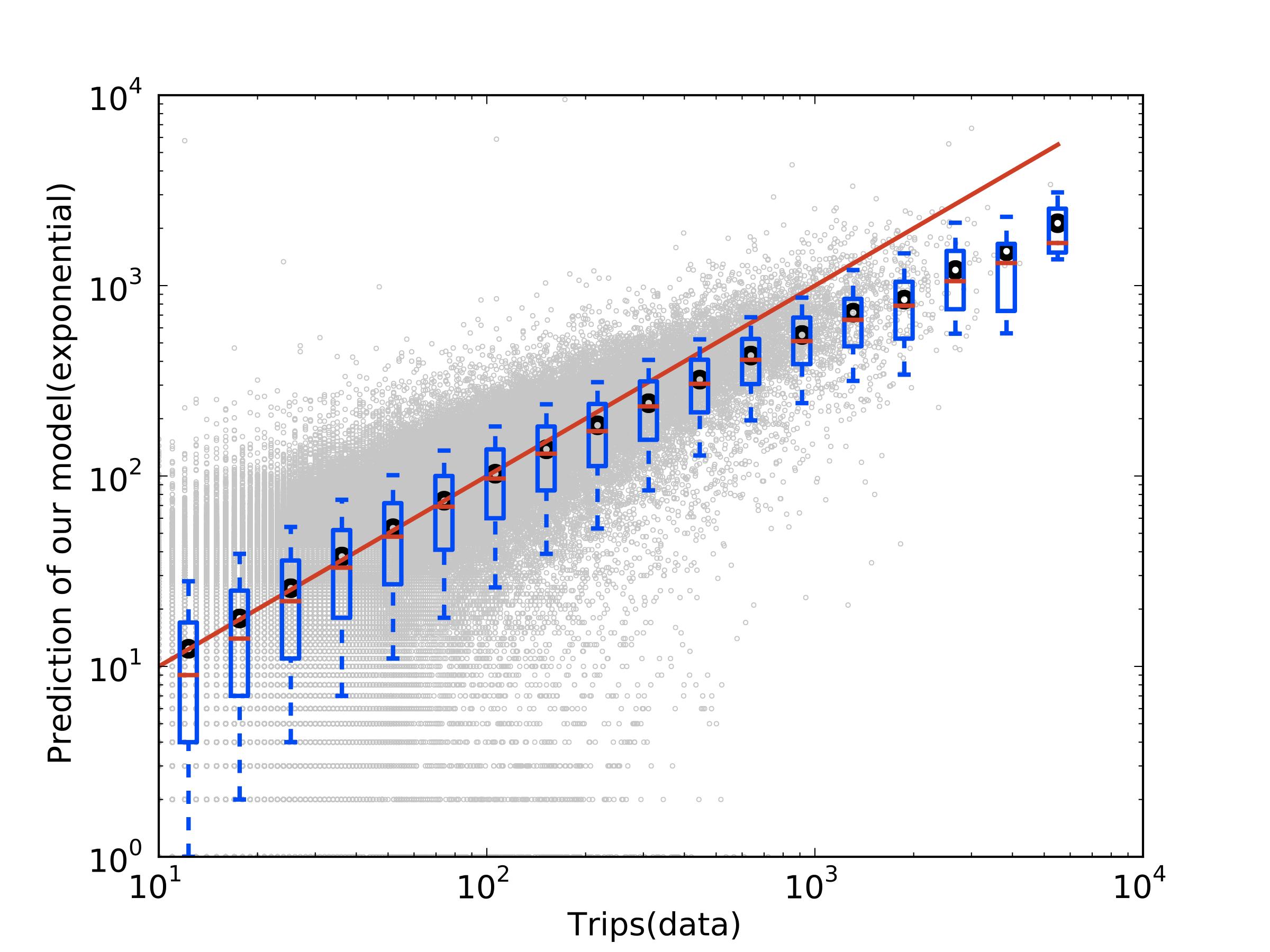
(d) Prediction by our model (exponential)

Figure 6: Simulations by the two forms of our model. (a-b) Distributions of trip length simulated by our model. (c-d) Prediction of traffic flows between cells by our model.

Subsequently, we apply our model to simulate trips by taxis in urban areas. The method of Maximum Likelihood Estimation (MLE) is used to evaluate the parameters in our model (see the appendix B for details). As for the two forms of function $f(d)$, the parameters $\sigma$ and $\lambda$ of our model are calculated as 1.601 and 0.308 respectively. The Fig. 6a and 6b, corresponding to the two forms of $f(d)$ in our model, both describe comparisons of distance distributions between simulated trips and actual ones. It can be seen that the distance distribution of trips predicted by our model with the form of power-law can accord with the actual ones very well and instead our model with the form of exponential underestimates the amount of trips with long distance. Furthermore, actual and predicted traffic flows between pairs of cells by the two forms of our model are shown in Fig. 6c and 6d. From the figures, it can be observed that the red line $y=x$ lies between the 9th and the 91st percentiles in bins in our model with the form of power-law, indicating that the model can predict the number of trips between cells accurately. But our model with the form of exponential may underestimate traffic flows. In summary, our model with the form of power-law can be treated as an appropriate model to predict traffic flows in urban areas. Thus, in the following paper, we only use our model with the form of power-law by default.

As demonstrated before, our model can be suitable to simulate human travels by taxis in urban areas. Whether is our model also applied to model collective human movement at large scale? Here, the dataset of US commuting is used, which described US commuting between United States countries in 2000 Simini2012a . As for our model, $P_{O}$ and $P_{D}$ shown in formula (3, 4) are replaced by the fractions of population in countries. The function $f(d)$ takes the form of power-law and $d$ is the distance between countries. So by using the method of MLE, it can be confirmed that the value of $\sigma$ is 3.077. In Fig. 7, the results of predicting the commuting number between pairs of counties by radiation model and our model are shown separately. Both models can predict the mobility patterns very well because both red lines almost fall between the 9th and 91st percentiles in each bin. In addition, observed from the gray points in the figure, the results predicted by our model seem more compact and have less fluctuations.

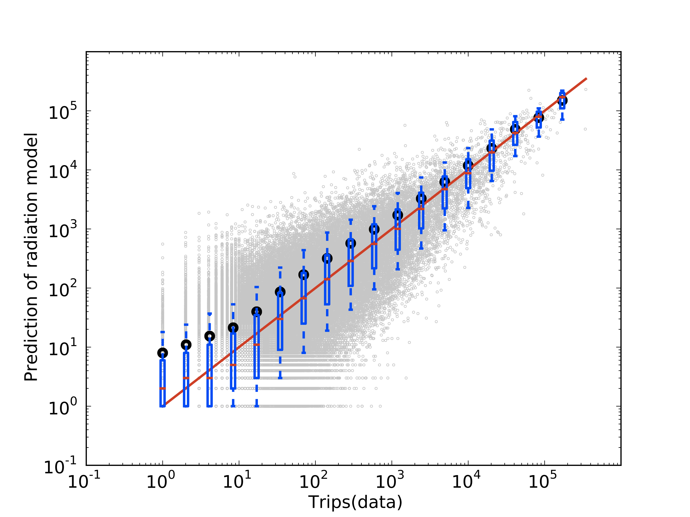
(a) Radiation model

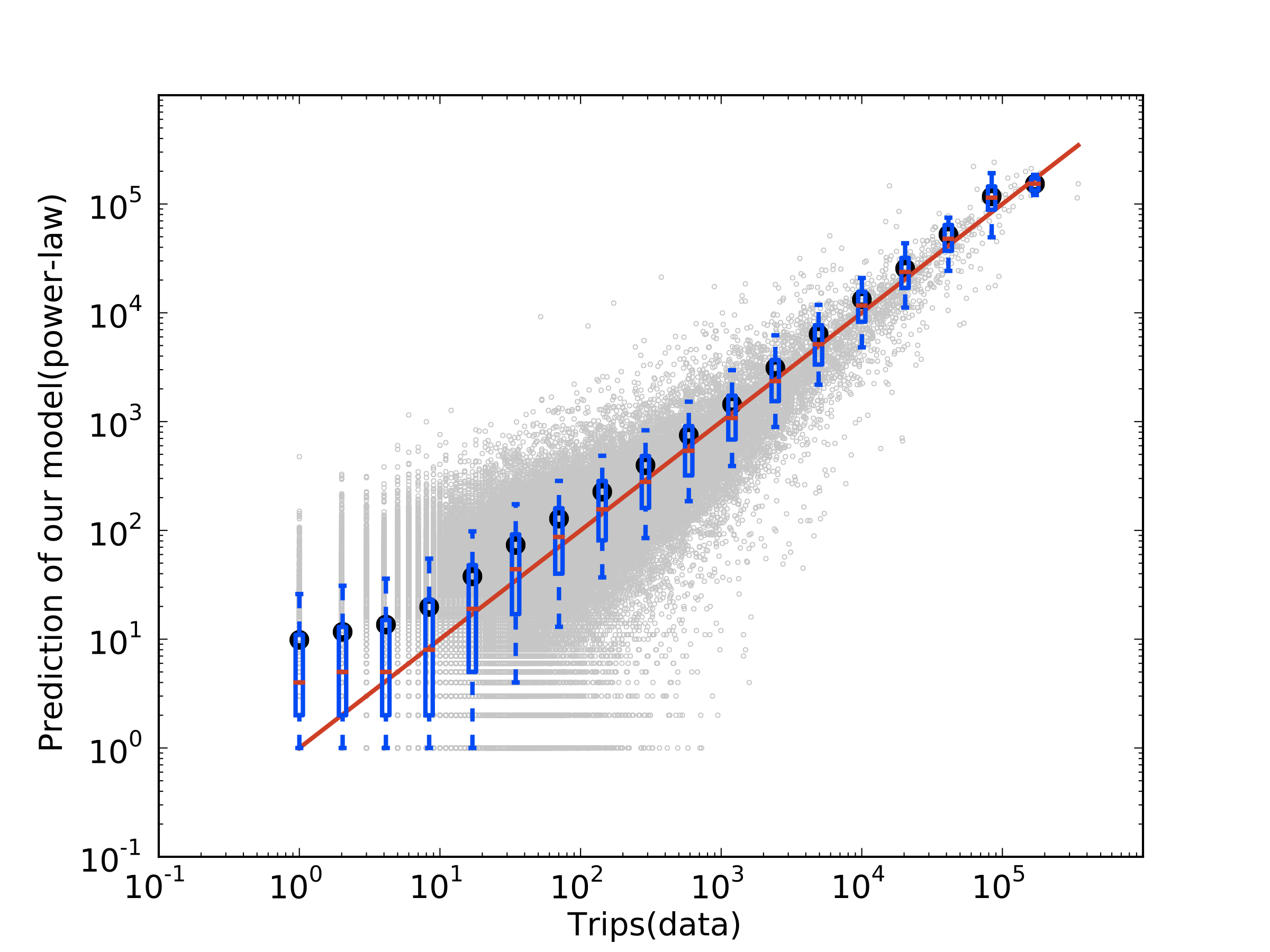
(b) Our model

Figure 7: Predictions on US commuting.

As a result, it is concluded that our model is very flexible and can simulate human movement not only in urban areas but also in countries.

III Analysis of distance distributions

In our model, $P_{O}$ and $P_{D}$, corresponding to distributions of origins and destinations, are probabilities of individuals’ leaving from and arriving at cells. For a whole day or longer time, both are almost equal and only depend on inherent properties of the city. So it is assumed that

$$P_{O}(i)=P_{D}(i)=P(i)\quad(i=1,\ldots,N),$$

where $P(\cdot)$ reflects human travel demands in grid cell regions.

Supporting the probability $P(\cdot)$ is uniform, the trips are simulated based on our model with two different values of $\sigma$ respectively (1.6, 2.4). As shown in Fig. 8, it can be seen that the distance distributions of trips in the two simulations accord to power-law with exponential cutoff very well. Actually, the exponential decay in the tail is caused by the geographic limits. The exponents of power-law in the two distributions are -0.713 for $\sigma=1.6$ (blue circles) and -1.486 for $\sigma=2.4$ (green triangles), which approach to the theoretical results as demonstrated in appendix C and will become more and more close to it as increasing the number of cells $N$. At the same time, the simulation according to actual distribution of travel demands in urban area of Beijing is also shown in the graph (red crosses), which is very close to the distribution of actual trip length. Compared with the simulations of uniform distribution, the travel distances decrease more rapidly even though the same value of $\sigma$.

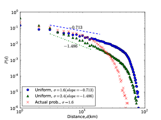
Figure 8: The simulations based on uniform distribution of human travel demands for different $\sigma$.

Then, considering the probability distribution of $P(\cdot)$ is the same as the actual one in Beijing, we only rearrange the probability values of grid cells randomly. As shown in Fig. 9a, the travels simulated on grid cells with randomized permuting probability values accord with power-laws in the heads and decay more slowly, compared with ones simulated on grid cells with actual travel demands. And in Fig. 9b, the two simulations based on actual travel demands reflected by taxis dataset and Sina Weibo dataset are shown respectively. It is illustrated that both distributions have similar trends in the head, but the tail of trips reflected by taxis dataset decreases more sharply. It is reasonable because, as described before, both geographic distributions of travel demands are similar near urban centers and the urban planning of Beijing expands during the two years.

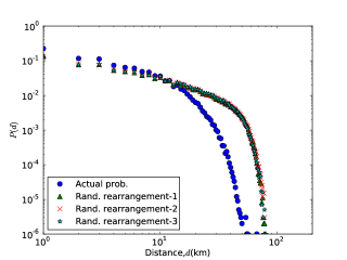
(a) Rearrangements

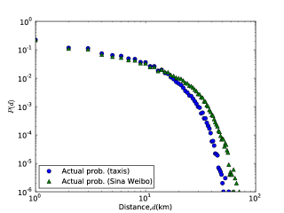
(b) Comparison

Figure 9: The simulations on different distributions. (a) Randomized rearrangements of actual probability distribution. (b) Comparison distributions of trip length based on actual probability distribution of taxis and Sina Weibo.

In conclusion, it suggests that not only the probability distribution of human travel demands, but also the layout of them is the fundamental element to account for collective human travel and determine the distribution of trip lengths. And they only depend on urban planning, population distribution and other properties of the city directly.

As illustrated above, it is no coincidence that exponential law is discovered in urban areas of cities. Then it is aimed to explore the origin of exponential law emerged in urban areas. Considering five hot spots regions in urban areas: Beijing West Railway Station (BWRS), Xizhimen, Beijing South Railway Station (BSRS), Sanlitun and Zhongguancun, the average densities of destinations or geo-tagged posts’ locations with distance from these regions are plotted in Fig. 10. From the Fig. 10a, the average densities for the five hot spots have similar trends and decay exponentially, in which the exponent of exponential is -0.256 and is not far from the value -0.230 observed from distance distribution shown in Fig. 2b. Also in Fig. 10b, the densities can be fitted by an exponential with exponent -0.231 when distances lie between 10km and 20km and then decay more quickly. It is worth mentioning that these findings seem like Clark’s Clark1951 who first use the negative exponential function to describe urban population density. These illustrate that the distributions of destinations and geo-tagged posts’ locations are very similar near centers of the city and these distributions may account for the exponential law in urban areas of cities.

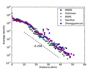
(a) Taxis

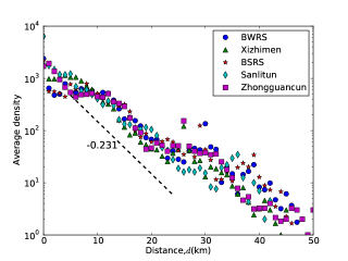
(b) Sina Weibo

Figure 10: The average densities of destinations and geo-tagged microblogs with distance from five hot spots regions in taxis and Sina Weibo datasets.

Therefore, assuming the density distributions are described by negative exponential functions for different exponents $\lambda$, we simulate human travels based on our model with the parameter $\sigma=1.601$. As shown in Fig. 11, different exponential exponents $\lambda$ about 0.25, 0.5 and 0.8 are considered. It is noticed that these distributions have obvious exponential decreasing trends, where the fitted exponents of tails of distributions are 0.200, 0.455 and 0.808 separately. As proved in appendix D, when the density function is exponential, the trip distance distribution $P(d)$ satisfies $C_{1}d^{1-\sigma}e^{-\lambda d}\leq P(d)\leq C_{2}d^{1-\sigma}e^{-\lambda d}$. So when $d>1/\lambda$, the exponential section dominates and $P(d)$ decreases exponentially. The fitted exponents are very close to the parameter $\lambda$ of density function, which accords with our theoretical proof very well. In urban areas, the density function usually decreases significantly leading to a large exponent $\lambda$. It must be noticed that the exponent of $d$ is usually larger than -1 because of the small parameter $\sigma$ for urban areas, which is different from the observed power-law distributions of distance where the exponents are between -2 and -1. So it can explain the reason why human trip distance in urban areas accords with exponential distribution more better.

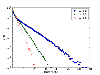
Figure 11: Simulations based on our model with average density distributions decreasing exponentially for different exponents.

IV Conclusions and future work

In our daily life, most human activities, especially movements, are concentrated in urban areas of cities. So it is very important to understand intra-city mobility patterns. In the paper, we aim to study human mobility patterns in urban areas through taxis dataset in Beijing.

Firstly, the geographic distributions of origins and destinations follow very similar patterns. And compared with geo-tagged microblogs’ locations, they are also very close each other near centers of the city. It suggests that these distributions are irrelevant to means of transport of human travels and only depend on urban planning, population distribution and other properties of the city.

Secondly, it seems that radiation model can not model collective human movement in urban areas very well. So we propose our model and observe the exponential law in the distribution of simulated trip lengths. Furthermore, our model may be appropriate for human travel not only in urban areas but in countries or larger ranges.

Finally, based on our model, it can be found that the distribution of trip distances depends on geographic distribution of human travel demands, which is inherent nature of the city. Meanwhile, it is observed that average human movement intensities decay exponentially with distance from hotspots. It can explain the origin of exponential law discovered in actual trip length distribution.

However, it must be emphasized that intra-urban mobility considered here occurred during a period of long time. In fact, the traffic flows between regions in urban areas is varied with the time of a day, which show strong periodic fluctuations. So in future, we will focus on the temporal characteristics of intra-urban individual flows to predict human mobility more precisely.

Appendix A Geo-tagged dataset of Sina Weibo

Microblogging services, such as Twitter and Weibo, have become more and more popular for users to share information with friends or followers. Recently, Weibo, Twitter and other online location-based services allow users to post their current geographic locations in messages. In Sina Weibo, when a user posts a geo-tagged microblog, it appears in a ”public timeline” of recent location updates. So by using Weibo’s geolocation API, we monitor the public timeline from Oct. 8, 2012 to Nov. 4, 2012 and only focus on the microblogs located in urban areas of Beijing. A total of 513315 geo-tagged posts are collected at first. After removing abnormal users and repeated microblogs posted by the same user in a relative short time, we finally obtain 491513 geo-tagged posts.

Appendix B MLE for our model

Let us consider intra-urban trips during a period of time, which can be denoted as $Tr=\{(l_{O}^{(r)},l_{D}^{(r)},t_{O}^{(r)},t_{D}^{(r)})|r=1,\ldots,n\}$, where $n$ is the number of trips. Supposing these trips are independent of each other, so the log probability of $Tr$ can be calculated as follows

$$\log{P(Tr)} = \log{\prod_{r=1}^{n}{P(l_{O}^{(r)}\to l_{D}^{(r)})}}$$

$$= \sum_{i,j,i\neq j}{T_{ij}\log{P(i\to j)}}$$

$$= \sum_{i,j,i\neq j}{T_{ij}\log{\frac{P_{O}(i)P_{D}(j)/f(d_{ij})}{\sum_{k\neq i}{P_{D}(k)/f(d_{ik})}}}}$$

$$= \sum_{i,j,i\neq j}{T_{ij}\log{\frac{P_{O}(i)P_{D}(j)}{M(i)f(d_{ij})}}}.$$

Here, the Nelder-Mead simplex algorithm Nelder01011965 is used to find the minimum of $-\log{P(Tr)}$ and evaluate the parameter $\sigma$ or $\lambda$ in the function $f(d)$ numerically.

Appendix C Proof of uniform density distribution

Supporting the probability $P(\cdot)$ is uniform (i.e. $P(i)=1/N$, $(i=1,\ldots,N)$), the probability with travel distance $d$ simulated based on our model can be denoted as

$$P(d) = \sum_{i,j:d_{ij}=d}{P(i\to j)}$$

$$= \sum_{i}{P(i)\sum_{j:d_{ij}=d}{\frac{P(j)/d^{\sigma}}{\sum_{k\neq i}{P(k)/d_{ik}^{\sigma}}}}},$$

where $d_{ij}$ represents the distance between cell $i$ and $j$, and $P(i)$ stands for the probability to select the cell $i$.

When $N$ is large, for different $i$, $\sum_{k\neq i}{P(k)/d_{ik}^{\sigma}}$ have approximately the same values. Therefore,

$$P(d)\propto N\cdot\frac{1}{N}\cdot d/d^{\sigma}\propto d^{1-\sigma}$$

Appendix D Proof of exponential density distribution

Figure 12: Illustration of negative exponential density function.

As shown in Fig. 12, the center is the point $O$ and the density distribution is

$$\rho(r)=Ce^{-\lambda r}\quad(0\leq r\leq R),$$

where $r$ is the distance from the center $O$ and $R$ is the size of a city. By using our model, we can estimate the displacement distribution of human movement as follows:

$$P(d)=\sum_{d(A,B)=d}{P(A\rightarrow B)}$$

Considering continuity of density distribution, it can also be written by

$$P(d)=\int\!\!\!\int\rho(A)\frac{\int_{s:d(A,B)=d}{\rho(B)d^{-\sigma}\mathrm{d}s}}{\int\!\!\!\int_{C\neq B}\rho(C)d(C,A)^{-\sigma}\mathrm{d}S_{2}}\mathrm{d}S_{1}$$

Let

$$I_{1}=\int_{s:d(A,B)=d}{\rho(B)d^{-\sigma}\mathrm{d}s}$$

and

$$I_{2}=\int\!\!\!\int_{C\neq B}\rho(C)d(C,A)^{-\sigma}\mathrm{d}S_{2}.$$

Therefore,

$$I_{1} = \int_{s:(x_{1}-x_{0})^{2}+(y_{1}-y_{0})^{2}=d}{Ce^{-\lambda\sqrt{x_{1}^{2}+y_{1}^{2}}}d^{-\sigma}\mathrm{d}s}$$

$$(x_{1}=x_{0}+d\cos{\alpha},y_{1}=y_{0}+d\sin{\alpha})$$

$$= \int_{0}^{2\pi}Cd^{1-\sigma}e^{-\lambda\sqrt{x_{0}^{2}+y_{0}^{2}+d^{2}+2d(x_{0}\cos{\alpha}+y_{0}\sin{\alpha})}}\mathrm{d}\alpha,$$

$$I_{2} = \int\!\!\!\int_{(x_{2},y_{2})\neq(x_{0},y_{0})}\frac{Ce^{-\lambda\sqrt{x_{2}^{2}+y_{2}^{2}}}}{(\sqrt{(x_{2}-x_{0})^{2}+(y_{2}-y_{0})^{2}})^{\sigma}}\mathrm{d}x_{2}\mathrm{d}y_{2}$$

$$(x_{2}=l\cos{\beta},y_{2}=l\sin{\beta})$$

$$= \int_{0}^{2\pi}\mathrm{d}\beta\int_{0}^{R}\frac{Cle^{-\lambda l}}{(\sqrt{l^{2}+x_{0}^{2}+y_{0}^{2}-2l(x_{0}\cos{\beta}+y_{0}\sin{\beta})})^{\sigma}}\mathrm{d}l.$$

$P(d)$ can be represented as

$$P(d) = \int\!\!\!\int Ce^{-\lambda\sqrt{x_{0}^{2}+y_{0}^{2}}}\frac{I_{1}}{I_{2}}\mathrm{d}x_{0}\mathrm{d}y_{0}$$

$$(x_{0}=r\cos{\theta},y_{0}=r\sin{\theta})$$

$$= \int_{0}^{2\pi}\mathrm{d}\theta\int_{0}^{R}Cre^{-\lambda r}\frac{U}{V}\mathrm{d}r$$

Where

$$U = \int_{0}^{2\pi}d^{1-\sigma}e^{-\lambda\sqrt{r^{2}+d^{2}+2dr\cos{(\theta-\alpha)}}}\mathrm{d}\alpha,$$

$$V = \int_{0}^{2\pi}\mathrm{d}\beta\int_{0}^{R}le^{-\lambda l}{(\sqrt{l^{2}+r^{2}-2rl\cos{(\beta-\theta)}})^{-\sigma}}\mathrm{d}l.$$

We notice that the denominator $V$ has nothing to do with $d$, so consider the numerator $U$

$$U = \int_{0}^{2\pi}d^{1-\sigma}e^{-\lambda\sqrt{r^{2}+d^{2}+2dr\cos{(\theta-\alpha)}}}\mathrm{d}\alpha$$

$$\geq \int_{0}^{2\pi}d^{1-\sigma}e^{-\lambda(r+d)}\mathrm{d}\alpha$$

$$= 2\pi d^{1-\sigma}e^{-\lambda d}e^{-\lambda r}.$$

In a similar way,

$$U \leq \int_{0}^{2\pi}d^{1-\sigma}e^{-\lambda\lvert r-d\rvert}\mathrm{d}\alpha$$

$$\leq \int_{0}^{2\pi}d^{1-\sigma}e^{-\lambda(d-r)}\mathrm{d}\alpha$$

$$= 2\pi d^{1-\sigma}e^{-\lambda d}e^{\lambda r}.$$

As a result,

$$C_{1}d^{1-\sigma}e^{-\lambda d}\leq P(d)\leq C_{2}d^{1-\sigma}e^{-\lambda d}$$

References

- (1) Duygu Balcan, Vittoria Colizza, Bruno Gonçalves, Hao Hu, José J Ramasco, and Alessandro Vespignani. Multiscale mobility networks and the spatial spreading of infectious diseases. Proceedings of the National Academy of Sciences of the United States of America, 106(51):21484–21489, 2009.
- (2) Marc Barthélemy. Spatial networks. Physics Reports, 499(1-3):1–101, 2011.
- (3) Armando Bazzani, Bruno Giorgini, Sandro Rambaldi, Riccardo Gallotti, and Luca Giovannini. Statistical laws in urban mobility from microscopic GPS data in the area of Florence. Journal of Statistical Mechanics: Theory and Experiment, 2010(05):P05001, May 2010.
- (4) D Brockmann, L Hufnagel, and T Geisel. The scaling laws of human travel. Nature, 439(7075):462–465, January 2006.
- (5) Colin Clark. Urban Population Densities. Journal of the Royal Statistical Society (Series A), 114(4):490–496, 1951.
- (6) Vittoria Colizza, Alain Barrat, Marc Barthelemy, Alain-Jacques Valleron, and Alessandro Vespignani. Modeling the worldwide spread of pandemic influenza: baseline case and containment interventions. PLoS Med, 4(1):e13, January 2007.
- (7) Segun Goh, Keumsook Lee, Jong Soo Park, and M. Y. Choi. Modification of the gravity model and application to the metropolitan Seoul subway system. Physical Review E, 86(2):026102, August 2012.
- (8) MC González, CA Hidalgo, and Albert-László Barabási. Understanding individual human mobility patterns. Nature, 453(7196):779–782, June 2008.
- (9) XP Han, Qiang Hao, BH Wang, and Zhou Tao. Origin of the scaling law in human mobility: Hierarchy of traffic systems. Physical Review E, 83(3):2–6, March 2011.
- (10) Yanqing Hu, Jiang Zhang, and Di Huan. Toward a general understanding of the scaling laws in human and animal mobility. EPL (Europhysics Letters), 96(3):38006, November 2011.
- (11) Bin Jiang, Junjun Yin, and Sijian Zhao. Characterizing the human mobility pattern in a large street network. Physical Review E, 80(2):1–11, August 2009.
- (12) Woo-Sung Jung, Fengzhong Wang, and H. Eugene Stanley. Gravity model in the Korean highway. Europhysics Letters, 81:48005, August 2008.
- (13) Pablo Kaluza, Andrea Kölzsch, Michael T Gastner, and Bernd Blasius. The complex network of global cargo ship movements. Journal of The Royal Society Interface, 7(48):1093–1103, 2010.
- (14) Chaogui Kang, Xiujun Ma, Daoqin Tong, and Yu Liu. Intra-urban human mobility patterns: An urban morphology perspective. Physica A: Statistical Mechanics and its Applications, 391(4):1702–1717, November 2012.
- (15) Gautier Krings, Francesco Calabrese, Carlo Ratti, and Vincent D Blondel. Urban gravity: a model for inter-city telecommunication flows. Journal of Statistical Mechanics: Theory and Experiment, 2009(07):L07003, July 2009.
- (16) Xiao Liang, Xudong Zheng, Weifeng Lv, Tongyu Zhu, and Ke Xu. The scaling of human mobility by taxis is exponential. Physica A: Statistical Mechanics and its Applications, 391(5):2135–2144, March 2012.
- (17) J A Nelder and R Mead. A Simplex Method for Function Minimization. The Computer Journal, 7(4):308–313, 1965.
- (18) Chengbin Peng, Xiaogang Jin, Ka-Chun Wong, Meixia Shi, and Pietro Liò. Collective Human Mobility Pattern from Taxi Trips in Urban Area. PLoS ONE, 7(4):e34487, 2012.
- (19) Camille Roth, Soong Moon Kang, Michael Batty, and Marc Barthélemy. Structure of urban movements: polycentric activity and entangled hierarchical flows. PLoS ONE, 6(1):e15923, January 2011.
- (20) Hernán D Rozenfeld, Diego Rybski, José S Andrade, Michael Batty, H Eugene Stanley, and Hernán A Makse. Laws of population growth. Proceedings of the National Academy of Sciences of the United States of America, 105(48):18702–18707, December 2008.
- (21) Filippo Simini, Marta C. González, Amos Maritan, and Albert-László Barabási. A universal model for mobility and migration patterns. Nature, 484:96–100, February 2012.
- (22) Chaoming Song, Tal Koren, Pu Wang, and Albert-László Barabási. Modelling the scaling properties of human mobility. Nature Physics, 6(10):818–823, September 2010.
- (23) Jameson L. Toole, Michael Ulm, Marta C. González, and Dietmar Bauer. Inferring land use from mobile phone activity. In Proceedings of the ACM SIGKDD International Workshop on Urban Computing - UrbComp ’12, pages 1–8, Beijing, China, 2012. ACM Press.
- (24) Marco Veloso, Santi Phithakkitnukoon, Carlos Bento, Nuno Fonseca, and Patrick Olivier. Exploratory Study of Urban Flow using Taxi Traces. In The First Workshop on Pervasive Urban Applications (PURBA), 2011.
- (25) Cécile Viboud, Ottar N Bjø rnstad, David L Smith, Lone Simonsen, Mark A Miller, and Bryan T Grenfell. Synchrony, Waves, and Spatial Hierarchies in the Spread of Influenza. Science, 312(5772):447–451, 2006.
- (26) Bing Wang, Lang Cao, Hideyuki Suzuki, and Kazuyuki Aihara. Safety-information-driven human mobility patterns with metapopulation epidemic dynamics. Scientific Reports, 2:887, January 2012.
- (27) A G Wilson. A statistical theory of spatial distribution models. Transportation Research, 1:253–269, 1967.
- (28) Jing Yuan, Yu Zheng, and Xing Xie. Discovering Regions of Different Functions in a City Using Human Mobility and POIs. In Proceedings of the 18th ACM SIGKDD international conference on Knowledge discovery and data mining, pages 186–194, Beijing, China, 2012. ACM.
- (29) Yu Zheng, Yanchi Liu, Jing Yuan, and Xing Xie. Urban computing with taxicabs. In Proceedings of the 13th international conference on Ubiquitous computing, pages 89–98, Beijing, China, 2011. ACM.