Shortcuts to adiabaticity by superadiabatic iterations

Abstract

Different techniques to speed up quantum adiabatic processes are currently being explored for applications in atomic, molecular and optical physics, such as transport, cooling and expansions, wavepacket splitting, or internal state control. Here we examine the capabilities of superadiabatic iterations to produce a sequence of shortcuts to adiabaticity. The general formalism is worked out as well as examples for population inversion in a two-level system.

I Introduction

There is currently much interest to speed up quantum adiabatic processes for applications such as fast cold-atom or ion transport, expansions, wave-packet splitting or internal state population and state control review . Different techniques have been put forward and/or applied. Among them Demirplack and Rice DR03 ; DR05 ; DR08 , and Berry Berry2009 proposed the addition of a suitable counterdiabatic term $H_{cd}^{(0)}(t)$ to the time dependent Hamiltonian $H_{0}(t)$ whose adiabatic dynamics is to be implemented. With that term added transitions in the instantaneous eigenbasis $\{|n_{0}(t)\rangle\}$ of $H_{0}(t)$ are suppressed, $H_{0}(t)|n_{0}(t)\rangle=E_{n}^{(0)}(t)|n_{0}(t)\rangle$, while there are in general transitions in the instantaneous eigenbasis of the new full Hamiltonian $H_{0}+H_{cd}^{(0)}$. Experiments that implement these ideas have been recently performed in different two-level systems Oliver ; Zhang . The same $H_{cd}^{(0)}(t)$ also appears naturally when studying the adiabatic approximation of the reference system, the one that evolves with $H_{0}(t)$, see e.g. Mes . The reference system behaves adiabatically, following the eigenstates of $H_{0}(t)$, when the counterdiabatic term is negligible, and the adiabatic approximation is close to the actual dynamics. This is made evident in an interaction picture (IP) based on the unitary transformation $A_{0}(t)=\sum_{n}|n_{0}(t)\rangle\langle n_{0}(0)|$. (The “parallel-transport” condition $\langle n_{0}(t)|\dot{n}_{0}(t)\rangle=0$ is assumed hereafter to define the phases.) From the Schrödinger equation $i\hbar\partial_{t}\psi_{0}(t)=H_{0}(t)\psi_{0}(t)$ and defining $\psi_{1}(t)=A_{0}^{\dagger}\psi_{0}(t)$, the IP equation $i\hbar\partial_{t}\psi_{1}(t)=H_{1}(t)\psi_{1}(t)$ is deduced, where $H_{1}(t)=A_{0}^{\dagger}(t)(H_{0}(t)-K_{0}(t))A_{0}(t)$ is the effective IP Hamiltonian and $K_{0}(t)=i\hbar\dot{A}_{0}(t)A_{0}^{\dagger}(t)$ is a coupling term. If $K_{0}(t)$ is zero or negligible, $H_{1}(t)$ becomes diagonal in the basis $\{|n_{0}(0)\rangle\}$, so that the IP equation becomes an uncoupled system with solutions

$$|\psi_{1}(t)\rangle=U_{1}(t)|\psi_{1}(0)\rangle,$$ (1)

where

$$U_{1}(t)=\sum_{n}|n_{0}(0)\rangle e^{-\frac{i}{\hbar}\int_{0}^{t}E_{n}^{(0)}(t^{\prime})dt^{\prime}}\langle n_{0}(0)|$$ (2)

is the unitary evolution operator for the uncoupled system. Correspondingly, from $|\psi_{0}(t)\rangle=A_{0}(t)|\psi_{1}(t)\rangle$,

$$|\psi_{0}^{(1)}(t)\rangle=\sum_{n}|n_{0}(t)\rangle e^{-\frac{i}{\hbar}\int_{0}^{t}E_{n}^{(0)}(t^{\prime})dt^{\prime}}\langle n_{0}(0)|\psi_{0}(0)\rangle,$$ (3)

where we have used $|\psi_{1}(0)\rangle=|\psi_{0}(0)\rangle$ since $A_{1}(0)=1$ by construction. The same solution, which, for a non-zero $K_{0}(t)$, is only approximate, may become exact by adding to the IP Hamiltonian the counterdiabatic term $A_{0}^{\dagger}(t)K_{0}(t)A_{0}(t)$. This requires an external intervention and changes the physics of the original system, so that $U_{1}(t)$ describes the evolution exactly. In the IP the modified Hamiltonian is $H^{(1)}(t)=H_{1}(t)+A_{0}^{\dagger}(t)K_{0}(t)A_{0}(t)=A_{0}^{\dagger}(t)H_{0}(t)A_{0}(t)$, and in the Schrödinger picture (SP) the additional term becomes simply $K_{0}$. The modified Schrödinger Hamiltonian is $H_{0}^{(1)}(t)=H_{0}(t)+K_{0}(t)$, so we identify $H_{cd}^{(0)}(t)=K_{0}(t)$. A “small” coupling term $K_{0}(t)$ that makes the adiabatic approximation a good one also implies a small counterdiabatic manipulation but, irrespective of the size of $K_{0}(t)$, $H_{0}^{(1)}(t)$ provides a shortcut to slow adiabatic following because it keeps the populations in the instantaneous basis of $H_{0}(t)$ invariant, in particular at the final time $t_{f}$. Moreover, if $K_{0}(0)=0$ and $K_{0}(t_{f})=0$, then $H_{0}^{(1)}=H_{0}$ at $t=0$ and $t=t_{f}$. This is useful in practice to ensure the continuity of the Hamiltonian at the boundary times: usually $H_{0}(t<0)=H_{0}(0)$ and $H_{0}(t>t_{f})=H_{0}(t_{f})$, so $K_{0}(t<0)=K_{0}(t>t_{f})=0$, i.e., $H_{0}(t)$ is the actual Hamiltonian before and after the process.

The previous formal framework may be repeated iteratively to define further IPs by diagonalizing the effective Hamiltonians of each IP. These iterations were used to establish generalized adiabatic invariants and adiabatic invariants of $n$-th order by Garrido Garrido . Berry also used this iterative procedure to calculate a sequence of corrections to Berry’s phase for cyclic processes with finite slowness, and introduced the concept of “superadiabaticity” Berry1987 . For later developments and applications see e.g. Berry1990 ; pertur ; Joli ; DR08 ; master ; MagReson ; Berry&Uzdin ; Uzdin&Moiseyev ; Moiseyev ; Oliver ; Sara12 .

The idea of superadiabatic iterations is best understood by working out explicitly the next interaction picture: let us start with $i\hbar\partial_{t}\psi_{1}(t)=H_{1}(t)\psi_{1}(t)$ and treat it as if it were, formally, a Schrödinger equation. The diagonalization of $H_{1}(t)$ provides the eigenbasis $\{|n_{1}(t)\rangle\}$, $H_{1}(t)|n_{1}(t)\rangle=E_{n}^{(1)}(t)|n_{1}(t)\rangle$, that we fix again with the parallel transport condition, $\langle n_{1}(t)|\dot{n}_{1}(t)\rangle=0$. A new unitary operator $A_{1}=\sum_{n}|n_{1}(t)\rangle\langle n_{1}(0)|$ plays now the same role as $A_{0}$ in the first (adiabatic) IP. It defines a new interaction picture wave function $\psi_{2}(t)=A_{1}^{\dagger}(t)\psi_{1}(t)$ that satisfies $i\hbar\partial_{t}\psi_{2}(t)=H_{2}(t)\psi_{2}(t)$, where $H_{2}(t)=A_{1}^{\dagger}(t)(H_{1}(t)-K_{1}(t))A_{1}(t)$ and $K_{1}=i\hbar\dot{A}_{1}A_{1}^{\dagger}$. If $K_{1}$ is zero or “small” enough, i.e., if a (first order) superadiabatic approximation is valid, the dynamics would be uncoupled in the new interaction picture, namely,

$$|\psi_{2}(t)\rangle=U_{2}(t)|\psi_{2}(0)\rangle,$$ (4)

where

$$U_{2}(t)=\sum_{n}|n_{1}(0)\rangle e^{-\frac{i}{\hbar}\int_{0}^{t}E_{n}^{(1)}(t^{\prime})dt^{\prime}}\langle n_{1}(0)|$$ (5)

is the approximate evolution operator in the second IP for uncoupled motion. It may happen that a process is not adiabatic, since $K_{0}(t)$ may not be neglected, but (first-order) superadiabatic when $K_{1}(t)$ can be neglected. Transforming back to the Schrödinger picture, $|\psi_{0}^{(2)}(t)\rangle=A_{0}(t)A_{1}(t)U_{2}(t)|\psi_{2}(0)\rangle$ becomes

$$|\psi_{0}^{(2)}(t)\rangle = \sum_{n}\sum_{m}|m_{0}(t)\rangle\langle m_{0}(0)|n_{1}(t)\rangle e^{-\frac{i}{\hbar}\int_{0}^{t}E_{n}^{(1)}(t^{\prime})dt^{\prime}}$$ (6)

$$\times \langle n_{1}(0)|\psi_{0}(0)\rangle,$$

and $|\psi_{2}(0)\rangle=|\psi_{0}(0)\rangle$ since $A_{0}(0)=A_{1}(0)=1$. Garrido distinguished two different aspects Garrido :

• Generalized adiabaticity: The evolution operator $A_{0}(t)A_{1}(t)U_{2}(t)$ provides an approximation to the actual (Schrödinger) dynamics up to a correction term of order $1/t_{f}^{2}$. This is so without imposing any boundary conditions (BCs) at $t=0$ and $t=t_{f}$ on the Hamiltonian $H_{0}$.

• Higher order adiabaticity: $A_{0}(t)A_{1}(t)U_{2}(t)$ does not guarantee in general that $|n_{0}(0)\rangle$ evolves into $|n_{0}(t_{f})\rangle$, up to a phase factor. If this is the objective, in other words, if a superadiabatic approximation should behave, at final times, like the adiabatic approximation, up to phase factors, then some BCs have to be imposed. Garrido discussed how generalized adiabaticity implies higher order adiabaticity when BCs at the boundary times are imposed on the derivatives of $H_{0}$.

(Garrido’s distinction does not apply in Berry1987 since there, it is assummed from the start that all the derivatives of the Hamiltonian $H_{0}$ vanish at the (infinite) time edges.) The second aspect is crucial to design shortcuts to adiabaticity for finite process times using the superadiabatic iterative structure, so let us be more specific. First notice that Eq. (6) becomes exact if the term $A_{1}^{{\dagger}}K_{1}A_{1}$ is added to the IP Hamiltonian, so that now the modified IP Hamiltonian is $H^{(2)}=H_{2}+A_{1}^{{\dagger}}K_{1}A_{1}=A_{1}^{{\dagger}}H_{1}A_{1}$. Then the modified SP Hamiltonian becomes $H_{0}^{(2)}(t)=H_{0}(t)+H_{cd}^{(1)}(t)$, where $H_{cd}^{(1)}(t)=A_{0}(t)K_{1}(t)A_{0}^{{\dagger}}(t)$. However, quite generally the populations of the final state (6) in the adiabatic basis $\{|n_{0}(t_{f})\rangle\}$ will be different from the ones of the adiabatic process, unless (a) $\{|n_{0}(0)\rangle\}=\{|n_{1}(t_{f})\rangle\}$, up to phase factors, and (b) $\{|n_{0}(0)\rangle\}=\{|n_{1}(0)\rangle\}$, also up to phase factors. (a) is satisfied when $K_{0}(t_{f})=0$. This makes $H_{1}(t_{f})$ diagonal in the basis $\{|n_{0}(0)\rangle\}$ and $[H_{1}(t_{f}),H_{0}(0)]=0$. (b) is satisfied when $K_{0}(0)=0$, which implies $H_{1}(0)=H_{0}(0)$. In summary the requirement is that the eigenstates of $H_{1}(t)$ at $t=0$ and $t=t_{f}$ coincide with the eigenstates of $H_{0}(0)$. If, in addition, $K_{1}(0)=K_{1}(t_{f})=0$, not only the populations, but also the initial and final Hamiltonians are the same for the “corrected” and for the reference processes, namely $H_{0}^{(2)}(0)=H_{0}(0)$ and $H_{0}^{(2)}(t_{f})=H_{0}(t_{f})$.

Further iterations define higher order superadiabatic frames with IP equations $i\hbar\partial_{t}\psi_{j}(t)=H_{j}\psi_{j}(t)$, where

$$H_{j} = A_{j-1}^{\dagger}(H_{j-1}-K_{j-1})A_{j-1},$$ (7)

$$K_{j} = i\hbar\dot{A}_{j}A_{j}^{\dagger},$$ (8)

with $A_{j}(t)=\sum_{n}|n_{j}(t)\rangle\langle n_{j}(0)|$ and $H_{j}(t)|n_{j}(t)\rangle=E_{n}^{(j)}(t)|n_{j}(t)\rangle$. As the $A_{j}(0)=1$ by construction, there is a common initial state $|\psi_{j}(0)\rangle=|\psi_{0}(0)\rangle$ for all iterations. The general form for the modified IP Hamiltonians is $H^{(j)}=H_{j}+A_{j-1}^{{\dagger}}K_{j-1}A_{j-1}=A_{j-1}^{{\dagger}}H_{j-1}A_{j-1}$. Thus, the form of the modified Hamiltonians in the SP is

$$H_{0}^{(j)}=H_{0}+H_{cd}^{(j-1)},$$ (9)

where the SP counterdiabatic term is

$$H_{cd}^{(j)}=B_{j}K_{j}B_{j}^{\dagger}=i\hbar B_{j}\dot{A}_{j}A_{j}^{\dagger}B_{j}^{\dagger},$$ (10)

with $B_{j}=A_{0}\cdot\cdot\cdot A_{j-1}$ and $B_{0}=I$. If $K_{j-1}(t)$ is small or negligible, $H_{j}(t)$ becomes diagonal in the basis $\{|n_{j-1}(0)\rangle\}$ and the IP equation becomes an uncoupled system with solutions $|\psi_{j}(t)\rangle=U_{j}(t)|\psi_{j}(0)\rangle$, where

$$U_{j}(t)=\sum_{n}|n_{j-1}(0)\rangle e^{-\frac{i}{\hbar}\int_{0}^{t}E_{n}^{(j-1)}(t^{\prime})dt^{\prime}}\langle n_{j-1}(0)|$$ (11)

is the approximate evolution operator in the $j$-th IP. Correspondingly, the approximate solution in the SP is given by $|\psi_{0}^{(j)}(t)\rangle=A_{0}(t)A_{1}(t)\cdot\cdot\cdot A_{j-1}(t)U_{j}(t)|\psi_{0}(0)\rangle$. This solution becomes exact if the $H_{cd}^{(j-1)}$ term is added to $H_{0}$, where in general the populations of $|\psi_{0}^{(j)}(t_{f})\rangle$ in the adiabatic basis $\{|n_{0}(t_{f})\rangle\}$ will be different from the ones of the adiabatic process, unless appropriate BCs are impossed. These boundary conditions are made explicit in the next section, and correspond partially to the conditions discussed by Garrido in Garrido to define “higher order adiabaticity”.

Is there any advantage in using one or another counter-diabatic scheme? There are several reasons that could make higher order schemes attractive in practice: one is that the structure of the $H_{cd}^{(j)}$ may change with $j$. For example, for a two-level atom population inversion problem, $H_{cd}^{(0)}=\hbar(\dot{\Theta}_{0}/2)\sigma_{y}$, whereas $H_{cd}^{(1)}=\hbar(\dot{\Theta}_{1}/2)(\cos\Theta_{0}\sigma_{x}-\sin\Theta_{0}\sigma_{z})$, where the $\Theta_{j}$ are the polar angles corresponding to the Cartesian components of the Hamiltonian $H_{j}$, and the $\sigma_{u}$, with $u=x,y,z$, are Pauli matrices Sara12 . (We shall use the Cartesian decomposition $X\sigma_{x}+Y\sigma_{y}+Z\sigma_{z}$ for different Hamiltonians below.)

A second reason is that, for a fixed process time, the cd-terms tend to be smaller in norm as $j$ increases, up to a value in which they begin to grow MagReson . An optimal iteration may thus be set Berry1990 ; MagReson . The “asymptotic character” of the superadiabatic coupling terms and the eventual divergence of the sequence can be traced back to the existence of non-adiabatic transitions, even if they are small Berry1987 .

To generate shortcuts one should pay attention though not only to the size of the cd-terms but also to the feasibility or approximate fulfillment of the required BCs at the boundary times. Thus, it may happen that an “optimal iteration”, of minimal norm for the cd-term, fails to provide a shortcut because of the BCs, as illustrated below in Sect. IV.

II Boundary conditions for shortcuts to adiabaticity via superadiabatic iterations

In this section we set the boundary conditions that guarantee that $H_{0}^{(j)}(t)$ provides a shortcut to adiabaticity. We have seen that for $j=1$ no conditions are required. For $j=2$ we need that $\{|n_{1}(t_{f})\rangle\}=\{|n_{0}(0)\rangle\}$ and $\{|n_{1}(0)\rangle\}=\{|n_{0}(0)\rangle\}$, (as before in these and similar expressions in brackets, the equalities should be understood up to phase factors), i.e., $K_{0}(t_{f})=K_{0}(0)=0$. For the iterations $j>2$ we need that (a) $\{|n_{j-1}(0)\rangle\}=\{|n_{0}(0)\rangle\}$, which occurs when $K_{j-2}(0)=K_{j-3}(0)=...=K_{1}(0)=K_{0}(0)=0$, and (b) $\{|n_{j-1}(t_{f})\rangle\}=\{|n_{j-2}(0)\rangle\}$, $\{|n_{j-2}(t_{f})\rangle\}=\{|n_{j-3}(0)\rangle\}$, $\{|n_{j-3}(t_{f})\rangle\}=\{|n_{j-4}(0)\rangle\}$, … , and $\{|n_{1}(t_{f})\rangle\}=\{|n_{0}(0)\rangle\}$. This amounts to imposing $K_{j-2}(t_{f})=K_{j-3}(t_{f})=...=K_{1}(t_{f})=K_{0}(t_{f})=0$. The vanishing of $K_{j^{\prime}}(0)$ for $j^{\prime}\leq j-2$ implies that $H_{0}(0)=H_{1}(0)=...=H_{j-1}(0)$, so (a) and (b) combined may be summarized as $\{|n_{j^{\prime}}(0)\rangle\}=\{|n_{j^{\prime}}(t_{f})\rangle\}=\{|n_{0}(0)\rangle\}$ for all $j^{\prime}\leq j-1$. Garrido showed that canceling out the first $l$-th time derivatives of $H_{0}(0)$ and $H_{0}(t_{f})$ makes $K_{j}(0)=0$ and $K_{j}(t_{f})=0$, for $j=1,...,l-1$, respectively Garrido . However canceling out the derivatives of $H_{0}$ is a sufficient but not a necessary condition to cancell the coupling terms, so we find it more useful to focus instead on the coincidence of the bases, this is exemplified in Sect. IV.

III Alternative framework with a constant basis

An alternative to the formal framework described so far provides computational advantages. It was implicity applied by Demirplak and Rice for a two-level system DR08 . We shall here generalize and formulate explicitly this approach and show its essential equivalence to the former. The main idea is to use instead of the $A_{j}$ a different set of unitary operators, $\tilde{A}_{j}(t)=\sum_{n}|\tilde{n}_{j}(t)\rangle\langle n|$, to define the sequence of interaction pictures, where $|\tilde{n}_{j}(t)\rangle$ are eigenstates of the new IP Hamiltonians $\tilde{H}_{j}(t)$, such that $\tilde{H}_{j}(t)|\tilde{n}_{j}(t)\rangle=\tilde{E}_{n}^{(j)}(t)|\tilde{n}_{j}(t)\rangle$, and $\{|n\rangle\}$ is a constant orthonormal basis equal for all $j$, which in principle does not necessarily coincide with $|n_{j}(0)\rangle$. Similarly to Eq. (7),

$$\tilde{H}_{j}=\tilde{A}_{j-1}^{\dagger}(\tilde{H}_{j-1}-\tilde{K}_{j-1})\tilde{A}_{j-1},$$ (12)

where $\tilde{K}_{j}=i\hbar\dot{\tilde{A}}_{j}\tilde{A}_{j}^{\dagger}=i\hbar\sum_{n}|\dot{\tilde{n}}_{j}(t)\rangle\langle\tilde{n}_{j}(t)|$. The counterdiabatic terms in the SP are introduced as before, $\tilde{H}_{cd}^{(j)}=\tilde{B}_{j}\tilde{K}_{j}\tilde{B}_{j}^{\dagger}$, where $\tilde{B}_{j}=\tilde{A}_{0}\cdot\cdot\cdot\tilde{A}_{j-1}$ with $\tilde{B}_{0}=I$. We shall next show that these cd-terms are independent of the chosen constant basis, so that $\tilde{H}_{cd}^{(j)}(t)=H_{cd}^{(j)}(t)$. Therefore, it is worth using $\tilde{A}_{j}(t)$ instead of $A_{j}(t)$ since they are simpler operators and significantly facilitate the manipulations as a common basis is used.

Let us start with the first iteration. Since $\tilde{H}_{0}(t)=H_{0}(t)$, then $\tilde{E}_{n}^{(0)}(t)=E_{n}^{(0)}(t)$, $|\tilde{n}_{0}(t)\rangle=|n_{0}(t)\rangle$, and $\tilde{K}_{0}=K_{0}$, so $\tilde{H}_{cd}^{(0)}=H_{cd}^{(0)}$. In addition, from Eq. (7), $H_{0}-K_{0}=A_{0}H_{1}A_{0}^{\dagger}$, and substituting it in Eq. (12) leads to

$$\tilde{H}_{1}=u_{0}H_{1}u_{0}^{\dagger},$$ (13)

where we have defined a constant unitary operator

$$u_{0} = \tilde{A}_{0}^{\dagger}A_{0}=\sum_{n}|n\rangle\langle n_{0}(0)|,$$

$$\dot{u}_{0} = 0.$$

Using

$$H_{j}(t)=\sum_{n}|n_{j}(t)\rangle E_{n}^{(j)}(t)\langle n_{j}(t)|$$ (14)

and

$$\tilde{H}_{j}(t)=\sum_{n}|\tilde{n}_{j}(t)\rangle\tilde{E}_{n}^{(j)}(t)\langle\tilde{n}_{j}(t)|,$$ (15)

for $j=1$ in Eq. (13), we get that $\tilde{E}_{n}^{(1)}(t)=E_{n}^{(1)}(t)$ and $|\tilde{n}_{1}(t)\rangle=u_{0}|n_{1}(t)\rangle$, while $|n\rangle=u_{0}|n_{0}(0)\rangle$. Expanding $\tilde{H}_{cd}^{(1)}=\tilde{A}_{0}\tilde{K}_{1}\tilde{A}_{0}^{\dagger}$ we have that

$$\tilde{H}_{cd}^{(1)}(t)=i\hbar\sum_{n,m,l,p}|\tilde{n}_{0}(t)\rangle\langle n|\dot{\tilde{m}}_{1}(t)\rangle\langle m|l\rangle\langle\tilde{l}_{1}(t)|p\rangle\langle\tilde{p}_{0}(t)|.$$

Using now $\langle m|l\rangle=\delta_{ml}$, $|\tilde{n}_{0}(t)\rangle=|n_{0}(t)\rangle$, $|n\rangle=u_{0}|n_{0}(0)\rangle$, and $|\tilde{n}_{1}(t)\rangle=u_{0}|n_{1}(t)\rangle$, it follows that $\tilde{H}_{cd}^{(1)}=H_{cd}^{(1)}$. Also, $\tilde{K}_{1}=\tilde{A}_{0}^{\dagger}A_{0}K_{1}A_{0}^{\dagger}\tilde{A}_{0}=u_{0}K_{1}u_{0}^{\dagger}$.

Repeating these steps for $j\geqslant 1$, $\tilde{H}_{j}=u_{j-1}H_{j}u_{j-1}^{\dagger}$ and $\tilde{K}_{j}=u_{j-1}K_{j}u_{j-1}^{\dagger}$, where

$$u_{j} = \tilde{A}_{j}^{\dagger}u_{j-1}A_{j}=\sum_{n}|n\rangle\langle n_{j}(0)|,$$

$$\dot{u}_{j} = 0.$$

This leads to $\tilde{E}_{n}^{(j)}(t)=E_{n}^{(j)}(t)$, $|\tilde{n}_{j}(t)\rangle=u_{j-1}|n_{j}(t)\rangle$, and $|n\rangle=u_{j-1}|n_{j-1}(0)\rangle$. Thus, for all $j\geq 0$,

$$\tilde{H}_{cd}^{(j)}=H_{cd}^{(j)}.$$

The boundary conditions to achieve shortcuts to adiabaticity take the same form as for the original framework in the previous section. Since $\tilde{K}_{0}=K_{0}$ and $\tilde{K}_{j}=u_{j-1}K_{j}u_{j-1}^{\dagger}$ for $j\geqslant 1$, for the $j$-th iteration, with $j>1$, we need that $\tilde{K}_{0}(0)=\tilde{K}_{1}(0)=...=\tilde{K}_{j-2}(0)=0$, and $\tilde{K}_{0}(t_{f})=\tilde{K}_{1}(t_{f})=...=\tilde{K}_{j-2}(t_{f})=0$. Let us recall that no conditions were required for $j=1$, although, as shown in the next section, using a convenient (constant or initial adiabatic) basis for specific Hamiltonians may also lead to conditions for $j=1$.

IV Two-level atom

The general formalism will now be applied to the two-level atom. Assuming a semiclassical interaction between a laser electric field and the atom, the electric dipole and the rotating wave approximations, the Hamiltonian of the system in a laser-adapted IP (that plays the role of the Schrödinger picture of the previous section) is

$$H_{0}(t)=\frac{\hbar}{2}\left(\begin{array}[]{cc}-\Delta(t)&\Omega_{R}(t)\\ \Omega_{R}(t)&\Delta(t)\end{array}\right),$$ (16)

where $\Omega_{R}(t)$ is the Rabi frequency, assumed real, and $\Delta(t)$ is the detuning, in the “bare basis” of the two level system, $|1\rangle=(\tiny{\begin{array}[]{c}1\\ 0\end{array}})$, $|2\rangle=(\tiny{\begin{array}[]{c}0\\ 1\end{array}})$. The Hamiltonians of the consecutive interaction pictures can be written as DR08

$$\tilde{H}_{j}(t)=\left(\begin{array}[]{cc}Z_{j}(t)&X_{j}(t)-iY_{j}(t)\\ X_{j}(t)+iY_{j}(t)&-Z_{j}(t)\end{array}\right),$$ (17)

or $\tilde{H}_{j}=X_{j}\sigma_{x}+Y_{j}\sigma_{y}+Z_{j}\sigma_{z}$ Sara12 . Then, $X_{0}(t)=\hbar\Omega_{R}(t)/2$, $Y_{0}(t)=0$ and $Z_{0}(t)=-\hbar\Delta(t)/2$. $X_{j}$, $Y_{j}$, and $Z_{j}$ are the Cartesian coordinates of the “trajectory” of $\tilde{H}_{j}(t)$. It is also useful to consider the corresponding polar, azimuthal and radial spherical coordinates, $\Theta_{j}(t)$, $\Phi_{j}(t)$, and $R_{j}(t)$ DR08 ; Sara12 , that satisfy

$$\cos(\Theta_{j}) = \frac{Z_{j}}{R_{j}},\,\,\,\,\sin(\Theta_{j})=\frac{P_{j}}{R_{j}},\,\,\,\,0\leq\Theta_{j}\leq\pi,$$

$$\cos(\Phi_{j}) = \frac{X_{j}}{P_{j}},\,\,\,\,\sin(\Phi_{j})=\frac{Y_{j}}{P_{j}},\,\,\,\,0\leq\Phi_{j}\leq 2\pi,\,\,\,\,\,\,\,\,$$ (18)

with $R_{j}=\sqrt{X_{j}^{2}+Y_{j}^{2}+Z_{j}^{2}}$ and $P_{j}=\sqrt{X_{j}^{2}+Y_{j}^{2}}$, where the positive branch is taken. The eigenvalues of $\tilde{H}_{j}(t)$ are $E_{1}^{(j)}=-R_{j}$ and $E_{2}^{(j)}=R_{j}$, and the corresponding eigenstates $\{|\tilde{n}_{j}(t)\rangle\}$ are

$$|\tilde{1}_{j}\rangle = e^{i\varepsilon_{j}}\left[e^{-i\Phi_{j}/2}\sin{\left(\frac{\Theta_{j}}{2}\right)}|1\rangle-e^{i\Phi_{j}/2}\cos{\left(\frac{\Theta_{j}}{2}\right)}|2\rangle\right],$$

$$|\tilde{2}_{j}\rangle = e^{-i\varepsilon_{j}}\left[e^{-i\Phi_{j}/2}\cos{\left(\frac{\Theta_{j}}{2}\right)}|1\rangle+e^{i\Phi_{j}/2}\sin{\left(\frac{\Theta_{j}}{2}\right)}|2\rangle\right],$$

where the phase

$$\varepsilon_{j}(t)=-\frac{1}{2}\int_{0}^{t}\dot{\Phi}_{j}(t^{\prime})\cos{[\Theta_{j}(t^{\prime})]}dt^{\prime}$$ (20)

is introduced to fulfill the parallel transport condition $\langle\tilde{n}_{j}|\dot{\tilde{n}}_{j}\rangle=0$. We define $\tilde{A}_{j}=|\tilde{1}_{j}(t)\rangle\langle 1|+|\tilde{2}_{j}(t)\rangle\langle 2|$. The matrix $\tilde{A}_{j}(t)$ under these conditions is

$$\tilde{A}_{j}=\left(\begin{array}[]{cc}\sin{\left(\frac{\Theta_{j}}{2}\right)}e^{i\varepsilon_{j}-i\Phi_{j}/2}&\cos{\left(\frac{\Theta_{j}}{2}\right)}e^{-i\varepsilon_{j}-i\Phi_{j}/2}\\ -\cos{\left(\frac{\Theta_{j}}{2}\right)}e^{i\varepsilon_{j}+i\Phi_{j}/2}&\sin{\left(\frac{\Theta_{j}}{2}\right)}e^{-i\varepsilon_{j}+i\Phi_{j}/2}\end{array}\right).$$ (21)

Then, from Eq. (8),

$$\tilde{K}_{j} = \frac{\hbar}{2}\left[-\dot{\Theta}_{j}\sin{\left(\Phi_{j}\right)}-\frac{\dot{\Phi}_{j}}{2}\cos{\left(\Phi_{j}\right)}\sin{\left(2\Theta_{j}\right)}\right]\sigma_{x}$$ (22)

$$+ \frac{\hbar}{2}\left[\dot{\Theta}_{j}\cos{\left(\Phi_{j}\right)}-\frac{\dot{\Phi}_{j}}{2}\sin{\left(\Phi_{j}\right)}\sin{\left(2\Theta_{j}\right)}\right]\sigma_{y}$$

$$+ \frac{\hbar\dot{\Phi}_{j}}{2}\sin^{2}{\left(\Theta_{j}\right)}\sigma_{z}.$$

Note that $\tilde{A}_{j}^{\dagger}\tilde{K}_{j}\tilde{A}_{j}=\tilde{A}_{j}^{\dagger}\dot{\tilde{A}}_{j}$ has only non-diagonal elements in the bare basis $\{|1\rangle,|2\rangle\}$ DR08 .

From Eq. (7), the Cartesian coordinates of $\tilde{H}_{j+1}(t)$ are

$$X_{j+1} = \frac{\hbar}{2}\left[\dot{\Theta}_{j}\sin{\left(2\varepsilon_{j}\right)}-\dot{\Phi}_{j}\sin{\left(\Theta_{j}\right)}\cos{\left(2\varepsilon_{j}\right)}\right],$$

$$Y_{j+1} = \frac{\hbar}{2}\left[-\dot{\Theta}_{j}\cos{\left(2\varepsilon_{j}\right)}-\dot{\Phi}_{j}\sin{\left(\Theta_{j}\right)}\sin{\left(2\varepsilon_{j}\right)}\right],$$

$$Z_{j+1} = -R_{j}.$$ (23)

In general, if $\Phi_{j}(t)$ is constant for a particular $j=J$, then $\dot{\Phi}_{J}(t)=0$, and from Eq. (20), $\varepsilon_{J}(t)=0$. Thus, taking into account Eq. (IV), we have that $X_{J+1}(t)=0$ and $Y_{J+1}(t)=-\hbar\dot{\Theta}_{J}/2$. Equation (IV) leads to $\Phi_{J+1}(t)=\{\pi/2,3\pi/2\}$, with $\pi/2$ when $Y_{J+1}>0$ ($\dot{\Theta}_{J}<0$), and $3\pi/2$ when $Y_{J+1}<0$ ($\dot{\Theta}_{J}>0$). If $Y_{J+1}=0$, $\Phi_{J+1}$ is discontinuous, and $\Theta_{J+1}=\pi$. Therefore, $\varepsilon_{J+1}(t)=\{0,\pm\pi/2\}$. From here, several general conditions can be deduced for $j^{\prime}>J$: $\Phi_{j^{\prime}>J}(t)=\{\pi/2,3\pi/2\}$, $\varepsilon_{j^{\prime}>J}(t)=\{0,\pm\pi/2\}$, $X_{j^{\prime}>J}(t)=0$, and $Y_{J+1}(t)=-\hbar\dot{\Theta}_{J}/2$ or $Y_{j^{\prime}>J+1}(t)=\pm\hbar\dot{\Theta}_{j^{\prime}-1}/2$. Moreover, from Eq. (22), $\tilde{K}_{j^{\prime}>J}=\pm(\hbar\dot{\Theta}_{j^{\prime}}/2)\sigma_{x}$ with positive sign if $\Phi_{j^{\prime}}(t)=3\pi/2$ and negative sign if $\Phi_{j^{\prime}}(t)=\pi/2$. Eq. (IV) and $Y_{0}(t)=0$ imply $\Phi_{0}(t)=0$ if $X_{0}(t)>0$ and $\Phi_{0}(t)=\pi$ if $X_{0}(t)<0$. We may thus take $J=0$ and apply the above relations, for example $\dot{\Phi}_{0}(t)=0$ and $\varepsilon_{0}(t)=0$.

As we mentioned before, the method fails as a shortcut to adiabaticity when the boundary conditions are not well fulfilled. In order to have a shortcut generated by the iteration $j$ we require that $\Delta(t)$ and $\Omega_{R}(t)$ are such that

$$|\tilde{1}_{j^{\prime}}(0)\rangle \approx |1\rangle,\,\,\,\,\,\,\,\,|\tilde{2}_{j^{\prime}}(0)\rangle\approx|2\rangle,$$ (24)

$$|\tilde{1}_{j^{\prime}}(t_{f})\rangle \approx |1\rangle,\,\,\,\,\,\,\,\,|\tilde{2}_{j^{\prime}}(t_{f})\rangle\approx|2\rangle,$$ (25)

for $0<j^{\prime}<j$, up to phase factors. For $j^{\prime}=0$ a natural and simple assumption is that the bare basis coincides initially with the adiabatic basis, i.e., Eq. (24); at $t_{f}$ we assume that the bare and adiabatic bases also coincide, allowing for permutations in the indices and phase factors.

At $t=0$, using Eq. (IV), taking into account that, from Eq. (20), $\varepsilon_{j^{\prime}}(0)=0$, and that $\Phi_{0}(t)=0$, $\sin{\left[\Theta_{j^{\prime}}(0)/2\right]}=1$ and $\cos{\left[\Theta_{j^{\prime}}(0)/2\right]}=0$ are required, or $\Theta_{j^{\prime}}(0)=\pi$. Then, $\cos{[\Theta_{j^{\prime}}(0)]}=Z_{j^{\prime}}(0)/R_{j^{\prime}}(0)=-1$. This condition is fulfilled if

$$Z_{j^{\prime}}^{2}(0)\gg X_{j^{\prime}}^{2}(0)+Y_{j^{\prime}}^{2}(0),$$ (26)

as long as $Z_{j^{\prime}=0}(0)<0$, and knowing that $Z_{j^{\prime}>0}(t)=-R_{j^{\prime}-1}(t)<0$. The condition (26) can be simplified for specific $j^{\prime}$-values as

$$|Z_{0}(0)| \gg |X_{0}(0)|,$$ (27)

$$|Z_{j^{\prime}>0}(0)| \gg |Y_{j^{\prime}>0}(0)|.$$ (28)

At $t=t_{f}$,

$$Z_{j^{\prime}}^{2}(t_{f})\gg X_{j^{\prime}}^{2}(t_{f})+Y_{j^{\prime}}^{2}(t_{f})$$ (29)

should be satisfied, where now, $\Theta_{0}(t_{f})$ can be either $0$, if $Z_{0}(t_{f})>0$, or $\pi$ if $Z_{0}(t_{f})<0$, and $\Theta_{j^{\prime}>0}(t_{f})=\pi$. As before, this condition splits into

$$|Z_{0}(t_{f})| \gg |X_{0}(t_{f})|,$$ (30)

$$|Z_{j^{\prime}>0}(t_{f})| \gg |Y_{j^{\prime}>0}(t_{f})|.$$ (31)

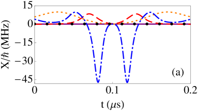
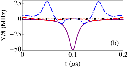
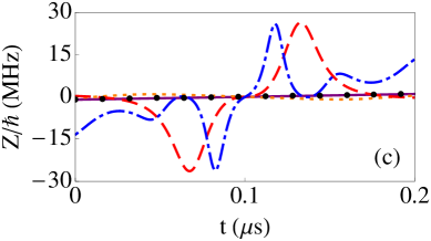
Figure 1: (Color online) The (a) $X$, (b) $Y$ and (c) $Z$ components for the Landau-Zener scheme, of: $H_{0}(t)$ (black dots), $H_{0}^{(1)}$ (purple solid line), $H_{0}^{(2)}$ (orange dotted line), $H_{0}^{(3)}$ (red dashed line), and $H_{0}^{(4)}$ (blue dot-dashed line). In (a) and (c) the black dots and the green thin line coincide and in (b) the black dots coincide with the orange dotted line. Parameters: $\alpha=-20$ MHz², $\Omega_{0,lz}=0.2$ MHz, and $t_{f}=0.2$ $\mu$s.

As an example we consider now a Landau-Zener scheme for $H_{0}$ (for the Allen-Eberly scheme we have found similar results), and study the behavior of $H_{0}^{(j)}$ with $j=1,2,3,4$, and the populations of the bare states driven by these Hamiltonians.

Table 1: Maxima of the X and Y components of $H_{0}$ and $H_{0}^{(j)}$ for $j=1,2,3,4,5$. Parameters: $\alpha=-20$ MHz², $\Omega_{0,lz}=0.2$ MHz, and $t_{f}=0.2$ $\mu$s.

Hamiltonian	$|X_{max}|/\hbar$ (MHz)	$|Y_{max}|/\hbar$ (MHz)
$H_{0}/\hbar$	0.1	0
$H_{0}^{(1)}/\hbar$	0.1	49.9
$H_{0}^{(2)}/\hbar$	10	0
$H_{0}^{(3)}/\hbar$	8.4	2.8
$H_{0}^{(4)}/\hbar$	46.8	28.1
$H_{0}^{(5)}/\hbar$	56.2	62.8

For the Landau-Zener model $\Delta(t)$ is linear in time and $\Omega_{R}(t)$ is constant,

$$\Delta_{lz}(t) = \alpha(t-t_{f}/2),$$

$$\Omega_{R,lz}(t) = \Omega_{0,lz},$$ (32)

where $\alpha$ is the chirp, and $\Omega_{0,lz}$ is a constant Rabi frequency. Condition (27) can be restated as

$$t_{f}\gg 2\left|\frac{\Omega_{0,lz}}{\alpha}\right|.$$ (33)

We consider the parameters $\alpha=-20$ MHz², $\Omega_{0,lz}=0.2$ MHz, and $t_{f}=0.2$ $\mu$s for which the dynamics with $H_{0}$ is non-adiabatic, see the Appendix A. Fig. 1 shows $X$, $Y$ and $Z$ components of $H_{0}$ and $H_{0}^{(j)}$, with $j=1,2,3,4$. In Figs. 1a and 1b and in table 1 we see that $H_{0}^{(2)}$ (corresponding to the first superadiabatic iteration) is optimal with respect to applied intensities. Moreover it cancells the $Y$-component completely, which is a simplifying practical advantage in some realizations of the two-level system Oliver ; Sara12 . From the second superadiabatic iteration both intensities start to increase again. For the parameters above, condition (33) is satisfied since $t_{f}=20\times|\Omega_{0,lz}/\alpha|$, but not so condition (28). Fig. 1 shows the disagreement between $H_{0}^{(j)}$ and $H_{0}$, at $t=0$ and $t=t_{f}$ for $j>1$. Fig. 2 shows that only $H_{0}^{(1)}=H_{0}+H_{cd}^{(0)}$ inverts the population of $|1\rangle$, $P_{1}(t)$, whereas the rest of the Hamiltonians fail to do so.

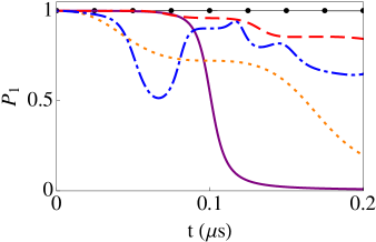
Figure 2: (Color online) Population of the state $|1\rangle$, $P_{1}(t)$, for the Hamiltonians $H_{0}(t)$ (black solid line with dots), $H_{0}^{(1)}$ (purple solid line), $H_{0}^{(2)}$ (orange dotted line), $H_{0}^{(3)}$ (red dashed line), and $H_{0}^{(4)}$ (blue dot-dashed line), with the Landau-Zener scheme. Parameters as in Fig. 1: $\alpha=-20$ MHz², $\Omega_{0,lz}=0.2$ MHz, and $t_{f}=0.2$ $\mu$s.

V Discussion

In this paper we have investigated the use of quantum superadiabatic iterations (a non-convergent sequence of nested interaction pictures) to produce shortcuts to adiabaticity. Each superadiabatic iteration may be used in two ways: (i) to generate a superadiabatic approximation to the dynamics, or (ii) to generate a counterdiabatic term that, when added to the original Hamiltonian, makes the approximate dynamics exact. The second approach, however, does not automatically generate shortcuts to adiabaticity, namely, a Hamiltonian that produces in a finite time the same final populations than the adiabatic dynamics. The boundary conditions needed for the second approach to generate a shortcut have been spelled out. This work is parallel to the investigation by Garrido to establish conditions so that the approach (i) provides an adiabatic-like approximation Garrido . We have also described an alternative framework to the usual set of superadiabatic equations which offers some computational advantages, and have applied the general formalism to the particular case of a two-level system. An optimal superadiabatic iteration with respect to the norm of the counterdiabatic term, is not necessarily the best shortcut, or in fact a shortcut at all, because of the possible failure of the boundary conditions.

We end by mentioning further questions worth investigating on the superadiabatic framework as a shortcut-to-adiabaticity generator. For example, other operations different from the population control of two-level systems (such as transport or expansions of cold atoms) have to be studied. Unitary transformations may be also applied to simplify the Hamiltonian structure making use of symmetries Sara12 . They have been discussed before as a way to modify the first (adiabatic) iteration Berry1990 ; Sara12 , and applied to perform a fast population inversion of a condensate in the bands of an optical lattice Oliver , but a systematic application and study, e.g. of the order with respect to the small (slowness) parameter, in particular for higher superadiabatic iterations, are still pending. A comparison with other methods to get shortcuts, at formal and practical levels would be useful too. A preliminary step in this direction, relating and comparing the invariant-based inverse engineering approach to the counterdiabatic approach of the first (adiabatic) iteration was presented in Inv_Berry , see also the Appendix B. Finally, comparisons among superadiabatic iterations themselves have to be performed, in particular regarding practical aspects such as the transient excitations involved energy .

We are grateful to O. Morsch and M. Berry for discussions. We acknowledge funding by Projects No. IT472-10, No. FIS2009-12773-C02-01, and the UPV/EHU program UFI 11/55. S. I. acknowledges Basque Government Grant No. BFI09.39. X. C. thanks the National Natural Science Foundation of China (Grant No. 61176118) and Grant No. 12QH1400800.

Appendix A Adiabaticity and boundary conditions for the Landau-Zener protocol

The adiabaticity condition for a two-level atom driven by the Hamiltonian (16) is Xi_PRL

$$\frac{1}{2}|\Omega_{a}(t)|\ll|\Omega(t)|,$$ (34)

where $\Omega_{a}(t)\equiv[\Omega_{R}(t)\dot{\Delta}(t)-\dot{\Omega}_{R}(t)\Delta(t)]/\Omega^{2}(t)$ and $\Omega=\sqrt{\Delta^{2}+\Omega_{R}^{2}}$. For the Landau-Zener scheme this condition takes the form

$$|\alpha|\ll 2\Omega_{0,lz}^{2}.$$ (35)

The inequalities that $\alpha$ must satisfy so that the system is adiabatic and also fulfills the boundary condition (33) are

$$2|\Omega_{0,lz}|/t_{f}\ll|\alpha|\ll 2\Omega_{0,lz}^{2}.$$ (36)

Fig. 3 shows the (shaded area) region for which $\alpha$ satisfies $20|\Omega_{0,lz}|/t_{f}<|\alpha|<0.2\Omega_{0,lz}^{2}$ when $t_{f}=2$ $\mu$s. No such area exists in the depicted domain for $t_{f}=0.2$ $\mu$s. For this shorter time the critical point where $1/t_{f}=\Omega_{0,lz}/100$ corresponds to $\Omega_{0,lz}=500$ MHz and detunings of up to $5$ GHz. Both may be problematic, as very large laser intensities and detunings could excite other transitions.

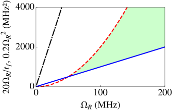
Figure 3: (Color online) $0.2\Omega_{0,lz}^{2}$ (red dashed line) and $20|\Omega_{0,lz}|/t_{f}$ (blue dashed line for $t_{f}=2$ $\mu$s and black dot-dashed line for $t_{f}=0.2$ $\mu$s). The shaded (green) area corresponds to values of $\alpha$ satisfying $20|\Omega_{0,lz}|/t_{f}<|\alpha|<0.2\Omega_{0,lz}^{2}$, namely, the process is adiabatic and the eigenstates at the boundary times are essentially the bare states. No such area exists for $t_{f}=0.2$ $\mu$s in the domain shown.

Appendix B Invariants

The superadiabatic sequence may be pictured as an attempt to find a higher order frame for which a coupling term $K_{j}$ is zero in the dynamical equation so that there are no transitions in some basis. This would mean that the states that the system follows exactly have been found, in other words, the eigenvectors of a dynamical invariant $I(t)$ Lewis_Riesenfeld ; Lewis_Leach ; Inv_Berry . When counter-diabatic terms are added, it is easy to construct invariants for $H_{0}^{(j)}$ from the instantaneous eigenstates of $H_{0}(t)$. However, quite generally this is not enough to generate a shortcut to adiabaticity because the boundary conditions to perform a quasi-adiabatic process (one that ends up with the same populations than the adiabatic one) may not be satisfied. A way out is to design the invariant first, and then $H(t)$ from it, satisfying the boundary conditions $[I(t),H(t)]=0$ at $t=0$ and $t=t_{f}$, and such that $H(0)=H_{0}(0)$ and $H(t_{f})=H_{0}(t_{f})$ Inv_Berry ; review .

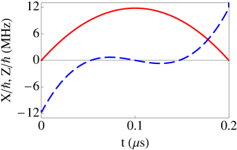
Figure 4: (Color online) $X$ (red solid line) and $Z$ (blue dashed line) components of the Hamiltonian obtained using the invariant-based inverse engineering method. $t_{f}=0.2$ $\mu$s.

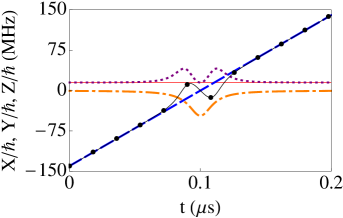
Figure 5: (Color online) The components $X_{0}(t)$ (red solid line) and $Z_{0}(t)$ (blue dashed line) of $H_{0}(t)$, the $Y(t)$ component of $H_{0}^{(1)}(t)$ (orange dot-dashed line), and the $X(t)$ (purple dotted line) and $Z(t)$ (black solid line with dots) components of $H_{0}^{(2)}$, for the Landau-Zener scheme. Parameters: $\alpha=-2800$ MHz², $\Omega_{0,lz}=30$ MHz, and $t_{f}=0.2$ $\mu$s.

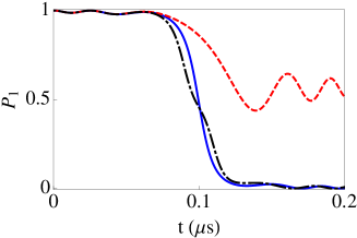
Figure 6: (Color online) Population of $|1\rangle$, $P_{1}(t)$, for the Hamiltonians $H_{0}(t)$ (red dashed line), $H_{0}^{(1)}$ (blue solid line), and $H_{0}^{(2)}$ (black dot-dashed line), with the Landau-Zener scheme. Parameters as in Fig. 5: $\alpha=-2800$ MHz², $\Omega_{0,lz}=30$ MHz, and $t_{f}=0.2$ $\mu$s.

For the general Hamiltonian in Eq. (16), a dynamical invariant of the corresponding Schrödinger equation may be parameterized as Inv_Berry

$$I(t)=\frac{\hbar}{2}\nu\left(\begin{array}[]{cc}\cos{\gamma(t)}&\sin{\gamma(t)}e^{i\beta(t)}\\ \sin{\gamma(t)}e^{-i\beta(t)}&-\cos{\gamma(t)}\end{array}\right),$$ (39)

where $\nu$ is an arbitrary constant with units of frequency to keep $I(t)$ with dimensions of energy. From the invariance condition for $I$,

$$\frac{dI(t)}{dt}\equiv\frac{\partial{I}(t)}{\partial{t}}-{\frac{i}{\hbar}}[I(t),H_{0}(t)]=0,$$ (40)

the functions $\gamma(t)$ and $\beta(t)$ must satisfy the differential equations

$$\dot{\gamma} = \Omega_{R}\sin\beta,$$

$$\dot{\beta} = \Delta+\Omega_{R}\cos\beta\cot\gamma.$$ (41)

To achieve a population inversion, the boundary values for $\gamma$ should be $\gamma(0)=0$ and $\gamma(t_{f})=\pi$. Assuming a polynomial ansatz shortcut_harmonic_traps ; transport ; Inv_Berry for $\gamma(t)$ and $\beta(t)$, as $\gamma(t)=\sum_{n=0}^{3}a_{n}t^{n}$ with the boundary conditions $\gamma(0)=\pi$, $\gamma(t_{f})=\dot{\gamma}(0)=\dot{\gamma}(t_{f})=0$, and $\beta(t)=\sum_{n=0}^{4}b_{n}t^{n}$ with the boundary conditions $\beta(0)=\beta(t_{f}/2)=\beta(t_{f})=-\pi/2$, $\dot{\beta}(t_{f})=-\pi/(2t_{f})$, and $\dot{\beta}(0)=\pi/(2t_{f})$, we can construct $\Delta$ and $\Omega_{R}$ Inv_Berry . These two functions are shown in Fig. 4, for $t_{f}=0.2$ $\mu$s ($\Omega_{R}=2X/\hbar$ and $\Delta=-2Z/\hbar$). For the same process time $t_{f}$ we also plot in Fig. 5 $X_{0}(t)$ and $Z_{0}(t)$ for a Landau-Zener protocol in which the Rabi frequency is slightly larger than the maximun required for the invariant-based protocol: $\Omega_{0,lz}=30$ MHz. As explained in the previous appendix, an unreasonably high laser intensity would be required to make it adiabatic while satisfying the bare-state condition at the edges, and $\Omega_{0,lz}=30$ MHz is still too small to satisfy Eq. (36). This is evident in the failure to invert the population, see Fig. 6. We use $\alpha=-2800$ MHz² to have the bare states as eigenvectors at the time edges which implies a rather large detuning. Fig. 5 also depicts the $Y(t)$ component of $H_{0}^{(1)}$ and the $X(t)$ and $Z(t)$ components of $H_{0}^{(2)}$ for $t_{f}=0.2$ $\mu$s. With these parameters these Hamiltonains provide shortcuts to adiabaticity, see Fig. 6, but they use very high detunings compared to those of the invariant-based protocol. This example does not mean, however, that invariant-based engineering is systematically more efficient. Invariant-based engineering and the counterdiabatic approach provide families of protocols that depend on the chosen interpolating auxiliary functions in the first case and on the reference Hamiltonian $H_{0}$ in the second. Their potential equivalence was studied in Inv_Berry .

References

(1) E. Torrontegui et al.,
Advances in Atomic, Molecular and Optical Physics, to be published (2013).
(2)M. Demirplak and S. A. Rice,
J. Phys. Chem. A 107, 9937 (2003).
(3)M. Demirplak and S. A. Rice,
J. Phys. Chem. B 109, 6838 (2005).
(4)M. Demirplak and S. A. Rice,
J. Chem. Phys. 129, 154111 (2008).
(5) M. V. Berry, J. Phys. A: Math. Theor. 42, 365303 (2009).
(6) M. G. Bason et al.
Nat. Phys. 8, 147 (2012).
(7) J. Zhang et al.,
arXiv:1212.0832.
(8) A. Messiah, Quantum Mechanics (Dover, New York 1999).
(9) L. M. Garrido, J. Math. Phys. 5, 355 (1964).
(10) M. V. Berry, Proc. R. Soc. Lond. A 414, 31 (1987).
(11) M. V. Berry, Proc. R. Soc. Lond. A 429, 61 (1990).
(12) K. Dresea and M. Holthausb, Eur. Phys. J. D 3, 73(1998).
(13) G. Dridi, S. Guérin, H. R. Jauslin, D. Viennot, and G. Jolicard,
Phys. Rev. A 82, 022109 (2010).
(14) J. Salmilehto and M. Möttönen,
Phys. Rev. B 84, 174507 (2011).
(15) M. Deschamps, G. Kervern, D. Massiot, G. Pintacuda, L. Emsley, and P. J. Grandinetti, J. Chem. Phys. 129, 204110 ̵͑(2008͒).
(16) M. V. Berry and R. Uzdin, J. Phys. A: Math. Theor. 44, 435303 (2011).
(17) R. Uzdin, A. Mailybaev, and N. Moiseyev, J. Phys. A: Math. Theor. 44, 435302 (2011).
(18) I. Gilary and N. Moiseyev, J. Phys. B: At. Mol. Opt. Phys. 45, 051002 (2012).
(19) S. Ibáñez, X. Chen, E. Torrontegui, J. G. Muga, and A. Ruschhaupt,
Phys. Rev. Lett. 109, 100403 (2012).
(20) X. Chen, E. Torrontegui, and J. G. Muga, Phys. Rev. A 83, 062116 (2011).
(21)X. Chen, J. G. Muga,
Phys. Rev. A 82, 053403 (2010).
(22) X. Chen, I. Lizuain, A. Ruschhaupt, D. Guéry-Odelin, and J. G. Muga, Phys. Rev. Lett. 105, 123003 (2010).
(23) H. R. Lewis and W. B. Riesenfeld, J. Math. Phys. 10, 1458 (1969).
(24) H. R. Lewis and P. G. L. Leach, J. Math. Phys. 23, 2371 (1982).
(25) X. Chen, A. Ruschhaupt, S. Schmidt, S. Ibáñez, and J. G. Muga, J. At. Mol. Sci. 1, 1 (2010).
(26) E. Torrontegui, S. Ibáñez, X. Chen, A. Ruschhaupt, D. Guéry-Odelin, and J. G. Muga, Phys. Rev. A 83, 013415 (2011).