Abstract

We present exact classical solutions of the higher-derivative theory that describes the dynamics of the position modulus of a probe brane within a five-dimensional bulk. The solutions can be interpreted as static or time-dependent throats connecting two parallel branes. In the nonrelativistic limit the brane action is reduced to that of the Galileon theory. We derive exact solutions for the Galileon, which reproduce correctly the shape of the throats at large distances, but fail to do so for their central part. We also determine the parameter range for which the Vainshtein mechanism is reproduced within the brane theory.

1 Introduction

Exact classical solutions of field theories are interesting as they can describe configurations that differ substantially from the usual perturbative vacuum. The purpose of this letter is to present a class of exact solutions of certain higher-derivative scalar theories in 3+1 dimensions. The theories have a geometric origin, as they describe hypersurfaces, which we term branes, embedded in a higher-dimensional spacetime. From the point of view of the brane observer the action involves only derivative terms of a particular form for one scalar degree of freedom.

We obtain our solutions by generalizing known static and time-dependent ones for the Dirac-Born-Infeld (DBI) theory with vanishing gauge fields. This theory can be viewed as the effective description of a $(3+1)$-dimensional brane embedded in a Minkowski bulk spacetime with one additional spatial dimension. A known static solution is the catenoidal configuration obtained by joining two branches with opposite first derivatives at the point where they display square-root singularities [1, 2]. The result is a smooth surface that looks like a throat or wormhole connecting two asymptotically parallel branes. A similar time-dependent solution describes two branes connected by a throat whose radius evolves with time. The throat shrinks to a minimal radius and subsequently re-expands [3, 4]. Alternatively, the square-root singularity can be viewed as a propagating shock front [5]. For the expanding configuration, energy is transferred from the location of the shock front, where the energy density diverges, to the region behind it.

We consider generalized theories that describe branes embedded in a flat bulk spacetime with one additional spatial dimension. The leading contribution to the action is given by the volume swept by the brane (the worldvolume), expressed in terms of the induced metric. It is invariant under arbitrary changes of the brane worldvolume coordinates. We eliminate this gauge freedom by identifying the brane coordinates with certain bulk coordinates (static gauge). The remaining bulk coordinate becomes a scalar field of the worldvolume theory, with dynamics governed by the DBI action. More complicated terms can also be included in the effective action. They can be expressed in terms of geometric quantities, such as the intrinsic and extrinsic curvatures of the hypersurface. In the static gauge these can be written in terms of the scalar field and its derivatives, so that we obtain a higher-derivative scalar theory with a particular structure of geometric origin [6, 7]. Some of the higher-derivative terms can be considered as quantum corrections to the DBI action [8].

The focus of our analysis is on brane theories constructed so that the equation of motion does not contain field derivatives higher than the second. In this way ghost fields do not appear in the spectrum. The most general scalar-tensor theory with this property was constructed a long time ago [9], and rediscovered recenty. It is characterized as the generalized Galileon (see ref. [10] and references therein). A particular example is provided by the Galileon theory [11], which results from the Dvali-Gabadadze-Porrati (DGP) model [12] in the decoupling limit. The connection with the brane picture is made in ref. [6], where it is shown that the Galileon theory can be reproduced in the nonrelativistic limit, starting from the effective action for the position modulus of a probe brane within a (4+1)-dimensional bulk.

2 The brane and Galileon theories

We consider the brane theory as formulated in ref. [6]. The induced metric on the brane in the static gauge is $g_{\mu\nu}=\eta_{\mu\nu}+\partial_{\mu}\pi\,\partial_{\nu}\pi$, where $\pi$ denotes the extra coordinate of the bulk space. Our convention for the Minkowski metric is $\eta_{\mu\nu}={\rm diag}(-1,1,1,1)$. The extrinsic curvature is $K_{\mu\nu}=-\partial_{\mu}\partial_{\nu}\pi/\sqrt{1+(\partial\pi)^{2}}$. We denote its trace by $K$. The leading terms in the brane effective action are [6]

$$S_{\lambda} = -\lambda\int d^{4}x\sqrt{-g}=-\lambda\int d^{4}x\sqrt{1+(\partial\pi)^{2}}$$ (1)

$$S_{K} = -M^{3}_{5}\int d^{4}x\sqrt{-g}\,K=M^{3}_{5}\int d^{4}x\,\left([\Pi]-\gamma^{2}[\phi]\right)$$ (2)

$$S_{R} = \frac{M^{2}_{4}}{2}\int d^{4}x\sqrt{-g}\,R=\frac{M^{2}_{4}}{2}\int d^{4}x\,\gamma\left([\Pi]^{2}-[\Pi^{2}]+2\gamma^{2}([\phi^{2}]-[\Pi][\phi])\right),$$ (3)

where $\gamma=1/\sqrt{-g}=1/\sqrt{1+(\partial\pi)^{2}}$. We have adopted the notation of ref. [6], with $\Pi_{\mu\nu}=\partial_{\mu}\partial_{\nu}\pi$ and square brackets representing the trace (with respect to $\eta_{\mu\nu}$) of a tensor. Also, we define $[\phi^{n}]\equiv\partial\pi\cdot\Pi^{n}\cdot\partial\pi$, so that $[\phi]=\partial^{\mu}\pi\,\partial_{\mu}\partial_{\nu}\pi\,\partial^{\nu}\pi$. We define the fundamental scale of the theory as $\Lambda=\lambda^{1/4}$. We express all dimensionful quantities in units of $\Lambda$ in numerical calculations. This is equivalent to setting $\lambda=1$.

The field equation of motion is [6]

$$\lambda\,\gamma\Bigl{\{}[\Pi]-\gamma^{2}[\phi]\Bigr{\}}-M^{3}_{5}\gamma^{2}\Bigl{\{}[\Pi]^{2}-[\Pi^{2}]+2\gamma^{2}\left([\phi^{2}]-[\Pi][\phi]\right)\Bigr{\}}$$

$$-\frac{M^{2}_{4}}{2}\gamma^{3}\Bigl{\{}[\Pi]^{3}+2[\Pi^{3}]-3[\Pi][\Pi^{2}]+3\gamma^{2}\left(2\left([\Pi][\phi^{2}]-[\phi^{3}]\right)-\left([\Pi]^{2}-[\Pi^{2}]\right)[\phi]\right)\Bigr{\}}=0.$$

(4)

The Galileon theory [11], which results from the DGP model [12] in the decoupling limit, can also be obtained by taking the nonrelativistic limit $(\partial\pi)^{2}\ll 1$ of the brane theory [6]. In this process, terms involving second derivatives of the field, such as $\Box\pi$, are not assumed to be small. If total derivatives are neglected, the leading terms in the expansion of eqs. (1)-(3) give [6]

$$S^{NR}=\int d^{4}x\,\Biggl{\{}-\frac{\lambda}{2}(\partial\pi)^{2}+\frac{M^{3}_{5}}{2}(\partial\pi)^{2}\Box\pi+\frac{M^{2}_{4}}{4}(\partial\pi)^{2}\left((\Box\pi)^{2}-(\partial_{\mu}\partial_{\nu}\pi)^{2}\right)\Biggr{\}}.$$ (5)

The term of highest order in the Galileon theory, omitted here, can be obtained by including in the brane action the Gibbons-Hawking-York term associated with the Gauss-Bonnet term of $(4+1)$-dimensional gravity. The theory can be put in more conventional form by defining $\lambda=\Lambda^{4}$ and employing the scalar field $\Lambda^{2}\pi$. As before, we express all quantities in units of $\Lambda$ in numerical calculations. The field equation of motion is

$$\lambda\,[\Pi]-M^{3}_{5}\left([\Pi]^{2}-[\Pi^{2}]\right)-\frac{M^{2}_{4}}{2}\left([\Pi]^{3}+2[\Pi^{3}]-3[\Pi][\Pi^{2}]\right)=0,$$ (6)

to be compared with eq. (4). The relation between the brane and Galileon theories implies the existence of solutions similar to the ones we described for the brane theory.

Before presenting solutions of the equations of motion, we must clarify an important point in their interpretation. We shall study configurations of two parallel branes, possibly connected by a throat. The form of the term (2), which is reduced to the second term of eq. (5) in the nonrelativistic limit, breaks the reflection symmetry across an isolated brane. In a two-brane system, it would affect differently the upper and lower parts of a throat, thus breaking the reflection symmetry across the middle plane between the two branes. The origin of this counterintuitive behavior can be traced to the DGP model [12]. In that construction, the brane corresponds to the boundary of the bulk space, and the field $\pi$ to a “brane-bending” mode. The two-brane configuration that we have in mind would correspond to a slab of bulk space of finite thickness, with two DGP branes on its sides. The long-distance physics will be affected by the effective compactification of the extra dimension. However, we are interested only in the range of scales that are relevant for the Galileon, which remain unaffected if we assume that the thickness of the slab of bulk space is sufficiently large. The “brane-bending” modes of the two branes are defined with respect to coordinate systems of opposite orientation along the extra dimension. If a unique coordinate system is used, one of the two modes must be shifted by the distance between the two branes and have its sign reversed. At the level of the Galileon theory, an equivalent way of describing the two-brane system is by assuming that the effective theory is given by eq. (5), but with opposite values of the coefficient $M^{3}_{5}$ of the cubic term for each of the two branes. The same assumption must be made for the term (2) of the brane theory, in order to get a two-brane configuration symmetric under reflection across the middle plane.

3 Solutions of the brane theory

A class of static solutions of eq. (4) can be obtained if we make the ansatz $\pi=\pi(w)$ with $w=r^{2}$. Eq. (4) becomes

$$\frac{\lambda}{\left(1+4w\pi_{w}^{2}\right)^{3/2}}\left(3\pi_{w}+8w\pi_{w}^{3}+2w\pi_{ww}\right) - \frac{4M^{3}_{5}\pi_{w}}{\left(1+4w\pi_{w}^{2}\right)^{2}}\left(3\pi_{w}+4w\pi_{w}^{3}+4w\pi_{ww}\right)$$ (7)

$$- \frac{12M^{2}_{4}\pi_{w}^{2}}{\left(1+4w\pi_{w}^{2}\right)^{5/2}}\left(\pi_{w}+2w\pi_{ww}\right)=0,$$

where the subscripts denote differentiation with respect to $w$.

For $M_{5}=M_{4}=0$ the action is reduced to the DBI one. In this case, the solution of the above equation is

$$\pi_{w}=\pm\frac{c}{\sqrt{w^{3}-4c^{2}w}},$$ (8)

with $c>0$. The two branches are depicted as dashed lines in figs. 1 and 2 for $c=10$. Integrating $\pi_{w}$ with respect to $w$ and joining the solutions smoothly at the location of the square-root singularity of eq. (8) generates a continuous double-valued function of $r$, which extends from infinite $r$ to $r_{th}=\sqrt{2c}$ and back to infinity. This catenoidal solution describes a pair of branes connected by a static throat [1, 2]. The integration constant $c$ is related to the total energy of the throat $E_{th}$. We have $E_{th}\sim c^{3/4}$, with $E_{th}$ and $c$ expressed in terms of $\Lambda$ [4]. The applicability of the effective brane theory for the description of the throat configuration requires $c\gg 1$ in the same units.

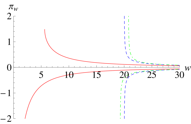
Figure 1: The solutions (8) (dashed), (11) (dot-dashed), (18) (solid) for $\kappa=1$, $c=10$.

The full equation (7) has similar solutions for nonvanishing $M_{5},M_{4}$. The general solution cannot be put in a simple analytical form. However, this is possible for special cases. For $\lambda=M_{4}=0$ the solution is

$$\pi_{w}=\pm\frac{c}{\sqrt{w^{3/2}-4c^{2}w}},$$ (9)

while for $\lambda=M_{5}=0$ it is

$$\pi_{w}=\pm\frac{c}{\sqrt{w}}.$$ (10)

Solutions with square-root singularities also exist for nonzero values of more that one of $\lambda$, $M_{5}$, $M_{4}$. For $M_{4}=0$ and $\kappa=12M^{3}_{5}/\lambda$ we find

$$\pi_{w}=\frac{\pm\sqrt{6}c}{\sqrt{3w^{3}+\sqrt{9w^{6}\mp 12\kappa c\,w^{9/2}}-24c^{2}w\mp 2\kappa c\,w^{3/2}}}.$$ (11)

This solution is reduced to eq. (8) for $\kappa=0$.

The solution (11) describes the modification of the throat in the presence of the higher-order term (2). The two branches of the solution (10) are depicted as dot-dashed lines in fig. 1 for $\kappa=1$, $c=10$, and in fig. 2 for $\kappa=40$, $c=10$. It is apparent that the location of the singularity is shifted in opposite directions for each of the two branches. The reason can be found in the form of the term (2), whose sign depends on the sign of the trace $K$ of the extrinsic curvature. As the latter is proportional to the second derivatives of the field $\pi$, the two branches have values of $K$ of opposite sign. We discussed this point at the end of the previous section, where we argued that in a two-brane configuration the brane actions must be characterized by opposite values of $M^{3}_{5}$. It can be checked easily that reversing the sign of $\kappa$ in eq. (11) generates the reflections across the horizontal axis of the two solutions depicted as dot-dashed lines in figs. (1), (2). In this way, two solutions of opposite $M^{3}_{5}$ can be joined smoothly at the common location of their singularities, for the construction of a catenoidal configuration.

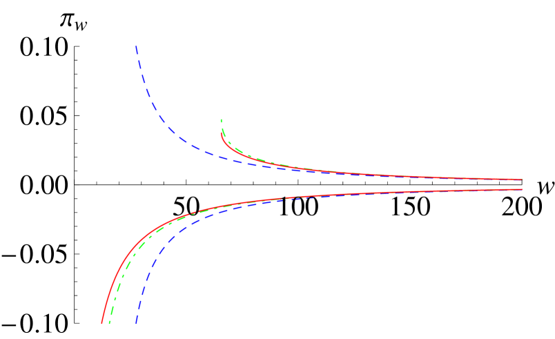
Figure 2: The solutions (8) (dashed), (11) (dot-dashed), (18) (solid) for $\kappa=40$, $c=10$.

In the following we shall focus on the branch corresponding to the lower signs in eq. (11), which allows us to make contact with the solution of the Galileon theory that realizes the Vainshtein mechanism. For large $w$ the solution falls off $\sim w^{-3/2}$, similarly to eq. (8). On the other hand, the inner part of the solution is affected by the presence of the higher-order term (2) in the effective action. The modification of the solution is small for large $c$, as can be seen in fig. 1. The singularity of this branch is located at $w_{th}=2c+\kappa(\kappa-\sqrt{288c+\kappa^{2}})/72$. For $c\to\infty$ we have $w_{th}\simeq 2c$, while for $c\to 0$, we have $w_{th}\simeq 144c^{2}/\kappa^{2}$.

A class of time-dependent solutions of eq. (4) can be obtained through the ansatz $\pi=\pi(z)$, with $z=r^{2}-t^{2}$. The field equation becomes

$$\frac{\lambda}{\left(1+4z\pi_{z}^{2}\right)^{3/2}}\left(2\pi_{z}+6z\pi_{z}^{3}+z\pi_{zz}\right) - \frac{12M^{3}_{5}\pi_{z}}{\left(1+4z\pi_{z}^{2}\right)^{2}}\left(\pi_{z}+2z\pi_{z}^{3}+z\pi_{zz}\right)$$ (12)

$$- \frac{12M^{2}_{4}\pi_{z}^{2}}{\left(1+4z\pi_{z}^{2}\right)^{5/2}}\left(2\pi_{z}+2z\pi_{z}^{3}+3z\pi_{zz}\right)=0,$$

where the subscripts denote differentiation with respect to $z$.

For $M_{5}=M_{4}=0$ the solution is [4]

$$\pi_{z}=\pm\frac{c}{\sqrt{z^{4}-4c^{2}z}},$$ (13)

with $c>0$. The two branches are depicted as dashed lines in fig. 3 for $c=10$. They possess square-root singularities at $z_{th}=(2c)^{2/3}$. Integrating $\pi_{z}$ with respect to $z$ we obtain two curves that can be joined smoothly at $z_{th}$. The resulting catenoidal solution $\pi(z)$ describes a pair of branes connected by a throat of radius $r_{th}=\sqrt{z_{th}+t^{2}}$. The throat starts with infinite radius for $t\to-\infty$, evolves down to a minimal size at $t=0$ and subsequently re-expands for positive $t$.

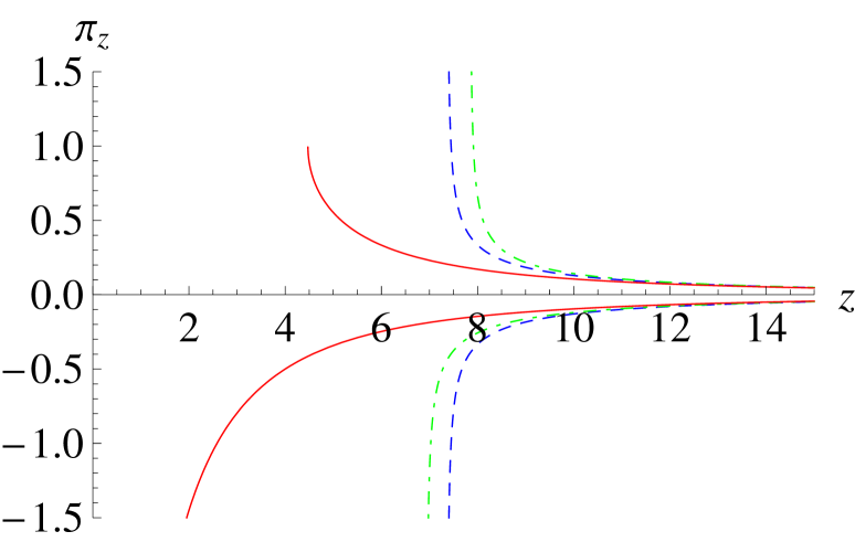
Figure 3: The solutions (13) (dashed), (16) (dot-dashed), (20) (solid) for $\kappa=1$, $c=10$.

The full equation (7) has similar solutions for nonvanishing $M_{5},M_{4}$. For $\lambda=M_{4}=0$ the solution is given by

$$\pi_{z}=\pm\frac{c}{\sqrt{z^{2}-4c^{2}z}},$$ (14)

while for $\lambda=M_{5}=0$ by

$$\pi_{z}=\pm\frac{c}{\sqrt{z^{4/3}-4c^{2}z}}.$$ (15)

Similarly to the static case, solutions with square-root singularities also exist for nonzero values of more that one of $\lambda$, $M_{5}$, $M_{4}$. For $M_{4}=0$ and $\kappa=12M^{3}_{5}/\lambda$ we find

$$\pi_{z}=\frac{\pm\sqrt{2}c}{\sqrt{z^{4}+z^{3}\sqrt{z^{2}\mp 2\kappa c}-8c^{2}z\mp\kappa c\,z^{2}}}.$$ (16)

This solution reproduces eq. (13) for $\kappa=0$. The two branches are depicted as dot-dashed lines in fig. 3 for $\kappa=1$, $c=10$. The construction of a catenoidal solution can be carried out in a way analogous to the static case. For large $z$ the solution (16) falls off $\sim z^{-2}$, similarly to eq. (13). On the other hand, the inner part is affected by the presence of the higher-order term (2).

4 Solutions of the Galileon theory

One of the most interesting features of the Galileon theory is revealed if we consider static, spherically symmetric solutions of the form $\pi=\pi(w)$, with $w=r^{2}$. The equation of motion (5) becomes

$$\lambda\left(3\pi_{w}+2w\pi_{ww}\right)-4M^{3}_{5}\pi_{w}\left(3\pi_{w}+4w\pi_{ww}\right)-12M^{2}_{4}\pi_{w}^{2}\left(\pi_{w}+2w\pi_{ww}\right)=0.$$ (17)

For $M_{4}=0$, $\kappa=12M^{3}_{5}/\lambda$ the solution is

$$\pi_{w}=\frac{3}{2\kappa}\left(1-\sqrt{1\mp\frac{4}{3}\frac{\kappa c}{w^{3/2}}}\right).$$ (18)

The two branches are depicted as solid lines in fig. 1 for $\kappa=1$, $c=10$, and in fig. 2 for $\kappa=40$, $c=10$. The branch with the upper sign terminates at the point $w=(4\kappa c/3)^{2/3}$. The branch with the lower sign displays the characteristic form associated with the Vainshtein mechanism. For $w\gg w_{V}$, with $w_{V}\sim(\kappa c)^{2/3}$ the square of the Vainshtein radius, the solution is $\pi_{w}\sim c\,w^{-3/2}$, so that $\pi\sim c/r$. On the other hand, for $w\ll w_{V}$, we have $\pi_{w}\sim\sqrt{c/\kappa}\,w^{-3/4}$, so that $\pi\sim\sqrt{c/\kappa}\,\sqrt{r}$. This solution requires the presence of a large point-like source at the origin with mass $\sim c$. The form of the solution at distances smaller than the Vainshtein radius results in the effective decoupling of fluctuations of the field $\pi$ induced by smaller energy sources [13]. The Galileon theory is applicable at length scales larger than 1 in units of the scale $\Lambda$. This means that the Vainshtein mechanism is operational only for large values of $\kappa c$ in the same units.

The correspondence between the brane solutions (8), (11) and the solution (18) of the Galileon theory is apparent in figs. 1 and 2. All solutions involve an integration constant and have the same asymptotic form at large distances. However, they deviate near the singularity of the brane solutions. A more precise correspondence can be found if we eliminate the term $\sim c^{2}$ in the denominator of eq. (11). The remaining terms can be rewritten as eq. (18). We thus conclude that the static solution of the Galileon theory can be obtained from the solution (11) of the brane theory in the formal limits $\kappa c\to\infty$ with $c$ held fixed, or $c\to 0$ with $\kappa c$ fixed. This formal correspondence does not constraint $c$ to be small in units of $\Lambda$. As is apparent from fig. 2, for $\kappa$ sufficiently larger than $c$, the brane and Galileon solutions almost coincide (apart from the location of the singularity) even for large $c$. For the theory of fig. 2 the Vainshtein radius is $w_{V}\simeq 66$. It is clear that the Vainshtein mechanism is operational within the brane picture as well, for sufficiently large $\kappa$. If we require $c\gg 1$ in units of $\Lambda$, the Vainshtein mechanism operates if $\kappa\gg c\gg 1$. It must be kept in mind, however, that large values of $\kappa$ indicate that the trilinear coupling of the $\pi$-field is large, so that quantum corrections are enhanced. The analysis of quantum corrections goes beyond the scope of this work. They have been discussed in ref. [14] for the Galileon theory and in ref. [8] for the brane theory.

Similarly to our analysis of the brane theory, we can obtain time-dependent solutions through the ansatz $\pi=\pi(z)$, with $z=r^{2}-t^{2}$. The field equation becomes

$$\lambda\left(2\pi_{z}+z\pi_{zz}\right)-12M^{3}_{5}\pi_{z}\left(\pi_{z}+z\pi_{zz}\right)-12M^{2}_{4}\pi_{z}^{2}\left(2\pi_{z}+3z\pi_{zz}\right)=0,$$ (19)

which should be compared with eq. (12) in the brane theory. We can obtain the solution analogous to eq. (16) by setting $M_{4}=0$ and defining $\kappa=12M^{3}_{5}/\lambda$. If we require that $\pi_{z}$ vanishes for $z\to\infty$, the solution is

$$\pi_{z}=\frac{1}{\kappa}\left(1-\sqrt{1\mp 2\frac{\kappa c}{z^{2}}}\right),$$ (20)

with $c>0$. Its asymptotic form for large $z$ matches that of eqs. (13) and (16). On the other hand, the two branches, displayed as solid lines in fig. 3 for $\kappa=1$, $c=10$, have completely different form for small $z$. The branch with the lower sign has a nonintegrable divergence at $z=0$, while the branch with the upper sign ceases to exist below $z=\sqrt{2\kappa c}$. It is difficult to give a physical interpretation to either case. For larger values of $\kappa$, the solutions (16) and (20) coincide for most of the range of $z$, apart from the region of the singularities. This behavior is similar to the one in the static case, depicted in fig. 2. The solutions (16), (20) become identical in the formal limits $\kappa c\to\infty$ with $c$ held fixed, or $c\to 0$ with $\kappa c$ fixed.

5 Discussion

In the context of the brane theory, the static solution can be interpreted as some type of sphaleron, with energy equal to the height of the barrier that must be overcome for the annihilation of the two-brane system [1, 4]. The time-dependent solution describes the dynamics of the annihilation process. Through analytical continuation to Euclidean space, this solution can be identified with the corresponding instanton. It must be kept in mind, however, that the spontaneous nucleation of the throat configuration may not be relevant for the annihilation of branes if these are identified with the D-branes of string theory. The annihilation of D-branes can take place through string processes at a rate faster than the one associated with the nucleation of a throat and its subsequent growth [1].

The form of the static and time-dependent solutions within the Galileon theory, eqs. (18) and (20) respectively, indicates that they are not appropriate for the description of the throat-nucleation process. The Galileon theory is an approximation to the DGP model which is expected to be valid at length scales larger than the inverse of the strong-coupling scale $\Lambda$. It is appropriate for the description of macroscopic effects, such as the decoupling of the scalar mode $\pi$ through the Vainshtein mechanism. However, it fails in regions in which a field configuration has large derivatives, such as near singularities. The embedding of the Galileon theory within a more complete framework, such as the brane theory, can resolve such problems. However, the brane theory cannot be viewed as the UV completion of the Galileon before its quantum properties are understood.

We note that it is possible to cut the two branches of all the solutions we discussed at a sufficiently large value $w_{b}$ or $z_{b}$ and join the outer segments. The resulting brane configuration would possess a kink at the location of the throat. This construction requires explicit boundary terms at $w_{b}$ or $z_{b}$, whose presence does not have an obvious justification.

The derivation of the solutions we presented was possible because of the special structure of the action of eqs. (1)-(3): Despite its apparent complexity, the field equation of motion (4) does not contain derivatives higher than the second. Moreover, the theory involves only derivatives of the field. For the ansatze we employed, which preserve the rotational or Lorentz symmetry by employing the invariants $r^{2}$ and $r^{2}-t^{2}$, the equation of motion becomes a first-order ordinary differential equation, such as (7) or (12), which can often be solved in closed form. This observation explains why theories with kinetic gravity braiding [15], as well as more general classes of derivative theories included in the generalized Galileon, can have similar solutions [16]. The interpretation of the solutions is not always easy, as in general they have singularities, while the theories do not have a geometric origin. One possibility is to identify the time-dependent solutions with propagating shock fronts, as in refs. [5, 3, 4]. The physics of such fronts depends sensitively on the details of the theory.

References

- [1] C. G. Callan and J. M. Maldacena, Nucl. Phys. B 513 (1998) 198 [hep-th/9708147].
- [2] G. W. Gibbons, Nucl. Phys. B 514 (1998) 603 [arXiv:hep-th/9709027]; [arxiv:hep-th/9801106].
- [3] J. Rizos and N. Tetradis, JHEP 1204 (2012) 110 [arXiv:1112.5546 [hep-th]].
- [4] J. Rizos and N. Tetradis, JHEP 1302 (2013) 112 [arXiv:1210.4730 [hep-th]].
- [5] W. Heisenberg, Zeit. Phys. Bd. 133, 3 (1952) 65.
- [6] C. de Rham and A. J. Tolley, JCAP 1005 (2010) 015 [arXiv:1003.5917 [hep-th]].
-
[7]
O. Aharony and M. Field,
JHEP 1101 (2011) 065 [arXiv:1008.2636 [hep-th]];
O. Aharony and M. Dodelson, JHEP 1202 (2012) 008 [arXiv:1111.5758 [hep-th]];
F. Gliozzi and M. Meineri, JHEP 1208 (2012) 056 [arXiv:1207.2912 [hep-th]]. - [8] A. Codello, N. Tetradis and O. Zanusso, JHEP 1304 (2013) 036 [arXiv:1212.4073 [hep-th]].
- [9] G. Horndeski, Int. J. Theor. Phys. 10 (1974) 363.
-
[10]
C. Deffayet, G. Esposito-Farese and A. Vikman,
Phys. Rev. D 79 (2009) 084003 [arXiv:0901.1314 [hep-th]];
C. Deffayet, X. Gao, D. A. Steer and G. Zahariade, Phys. Rev. D 84 (2011) 064039 [arXiv:1103.3260 [hep-th]];
T. Kobayashi, M. Yamaguchi and J. ’i. Yokoyama, Prog. Theor. Phys. 126 (2011) 511 [arXiv:1105.5723 [hep-th]];
C. Charmousis, E. J. Copeland, A. Padilla and P. M. Saffin, Phys. Rev. Lett. 108 (2012) 051101 [arXiv:1106.2000 [hep-th]]. - [11] A. Nicolis, R. Rattazzi and E. Trincherini, Phys. Rev. D 79 (2009) 064036 [arXiv:0811.2197 [hep-th]].
-
[12]
G. R. Dvali, G. Gabadadze and M. Porrati,
Phys. Lett. B 485 (2000) 208 [hep-th/0005016];
C. Deffayet, G. R. Dvali and G. Gabadadze, Phys. Rev. D 65 (2002) 044023 [astro-ph/0105068]. -
[13]
A. I. Vainshtein,
Phys. Lett. B 39 (1972) 393;
E. Babichev and C. Deffayet, arXiv:1304.7240 [gr-qc]. -
[14]
A. Nicolis and R. Rattazzi,
JHEP 0406 (2004) 059 [hep-th/0404159];
K. Hinterbichler, M. Trodden and D. Wesley, Phys. Rev. D 82 (2010) 124018 [arXiv:1008.1305 [hep-th]];
C. de Rham, G. Gabadadze, L. Heisenberg and D. Pirtskhalava, Phys. Rev. D 87 (2013) 085017 [arXiv:1212.4128 [hep-th]]. -
[15]
C. Deffayet, O. Pujolas, I. Sawicki and A. Vikman,
JCAP 1010 (2010) 026 [arXiv:1008.0048 [hep-th]];
O. Pujolas, I. Sawicki and A. Vikman, JHEP 1111 (2011) 156 [arXiv:1103.5360 [hep-th]]. - [16] A. Vikman, private communication.