Maximum Likelihood Estimation for Conditionally Heteroscedastic Models when the Innovation Process is in the Domain of Attraction of a Stable Law

Abstract

We prove the strong consistency and the asymptotic normality of the maximum likelihood estimator of the parameters of a general conditionally heteroscedastic model with $\alpha$-stable innovations. Then, we relax the assumptions and only suppose that the innovation process converges in distribution toward a stable process. Using a pseudo maximum likelihood estimator with a stable density, we also obtain the strong consistency and the asymptotic normality of the estimator. This framework seems relevant for financial data exhibiting heavy tails. We apply this method to several financial index and compute stable Value-at-Risk.

JEL Classification: C12, C13 and C22

Keywords: Conditional Heteroscedasticity, Maximum Likelihood Estimation, Stable Law, Domain of attraction, Value-at-Risk.

1 Introduction

ARCH models, introduced by Engle (1982) and generalized by Bollerslev (1986) are some of the most popular models for explaining financial time series. In these models, the time series is stationary but possesses a time varying conditional variance, this property can be used to explain some of the stylized facts that can be found in financial series. The GARCH modeling explains the volatility clustering but it also explains a fraction of the leptokurticity that can be found in financial time series. Empirical evidences can be found in the survey article by Shephard (1996). The most widely used estimator for the parameters of the GARCH model is the Gaussian Quasi Maximum Likelihood Estimator (QMLE). To implement this estimator, the Gaussian density is used to compute the likelihood of the model, even if the exact distribution of the error process remains unspecified. Under appropriate assumptions, the Gaussian QMLE is Consistent and Asymptotically Normal (CAN), see Berkes et al. (2003) or Francq and Zakoïan (2004).

Most of the assumptions required for the Gaussian QMLE to be CAN are mild, since one does not need to specify the true distribution of the error process, the model is less risky to be misspecified as in the Maximum Likelihood Estimation (MLE) case. The only assumption that can be challenged is the requirement that the error process possesses a finite fourth moment. The GARCH model and its derivatives are mostly applied to financial data which are known to be heavy tailed. Mandelbrot (1963) and Fama (1965) found that the unconditional distributions of most financial returns are heavy tailed and therefore do not necessarily possess a finite fourth moment. Now even if the GARCH modeling explains a part of the leptokurticity of the financial time series, the residuals are often found to remain heavy tailed. For this reason, there were several attempts to use GARCH models with non-Gaussian innovation, see Berkes and Horváth (2004) for a general approach. GARCH models with heavy tailed distributions have been studied, Bollerslev (1987) use the student t distribution and Liu and Brorsen (1995) used an $\alpha$-stable distribution for the error process and studied the model empirically, see also Mittnik and Paolella (2003), Embrechts et al. (1997).

In this paper we study a stable Maximum Likelihood Estimator (MLE) of a general conditionally heteroskedastic model in which the errors follow a stable distribution. To the best knowledge of the author, the CAN property of the MLE of such a model with stable innovation has not been proven, even in the GARCH case where the model was only studied empirically. Here we prove such a result under a few assumptions about the functional form of the volatility process. By specifying the distribution of the error process $(\eta_{t})_{t}$ to be $\alpha$-stable, we obtain a less general method than the Gaussian QMLE but we do not need any moment assumption and the model takes into account the fact the data can be heavy tailed.

The Gaussian QMLE possesses the robustness property that even if the errors are not Gaussian, provided that their distribution is in the domain of attraction of the Gaussian law, the QML estimator is still CAN. We want to obtain a similar property for the stable GARCH model. Since the only probability distributions to possess a domain of attraction are the Gaussian distribution and the family of stable laws, we use this fact to obtain a robustness property for the stable estimation. In other words, we study the asymptotic behavior of the MLE written for stable innovations when the error process is not stable but close to a stable distribution. With the Generalized Central Limit Theorem (GCLT) (see Gnedenko et al. (1968)), we can characterize the domain of attraction of a stable law. A sum of i.i.d random variables with certain properties will converge in distribution to a stable variable. If the innovation process can be written as a sum of variables, then if the sum converges, it converges in distribution toward a stable law. We use this property to give a more general result than the stable MLE. We prove that if the innovation process is not stable but converges in distribution to a stable variable, then the stable MLE (which in this case is a pseudo MLE) is still CAN.

We will study a general class a conditionally heteroscedastic model, defined by

$$\left\{\begin{aligned} \epsilon_{t}&=\sigma_{t}\eta_{t}\\ \sigma_{t}&=g\left(\epsilon_{t-1},\epsilon_{t-2},\ldots;\theta_{0}\right),\end{aligned}\right.$$ (1.1)

where $(\epsilon_{t})_{t}$ is the observed process ( $\epsilon_{t}\in\mathbb{R}$), $(\eta_{t})_{t}$ is a sequence of independent and identically (i.i.d) random variables (the error process), $\theta_{0}$ is a parameter belonging to a parameter space $\Theta$ and $g:\ \mathbb{R}^{\infty}\times\Theta\mapsto\mathbb{R}_{+}^{*}$. This model contains most of the numerous derivatives of the GARCH model that have been introduced such as EGARCH, TGARCH and many others, see Bollerslev (2008) for a exhaustive (at the time) list. Model (1.1) contains the classical GARCH$(p,q)$ model given by

$$\sigma_{t}^{2}=\omega+\sum_{i=1}^{q}a_{i}\epsilon_{t-i}^{2}+\sum_{j=1}^{p}b_{j}\sigma_{t-j}^{2}.$$ (1.2)

The plan of this paper is as follows. We recall useful results concerning the stable distribution in Section 2. In the third section, we study a conditional heteroscedastic model with stable innovation and prove that the MLE is stable. In Section 4, we consider the case where the stable density is used to compute a pseudo MLE when the error process is not stable but converges in distribution toward a stable process. Then, we present in Section 5 some simulation results and some financial applications.

2 Properties of stable distributions

Since the pioneer work of Mandelbrot, the class of stable distributions is commonly used in finance and in other areas such as engineering, signal processing and many other. There are empirical evidences that some financial processes, denoted $(X_{t})_{t}$, have regularly varying (heavy) tails, that is, $\mathbb{P}\left[X_{t}>x\right]\sim Kx^{-\alpha}$, when $|x|\rightarrow+\infty$, where $K$ is a constant and $\alpha\in\left(0,2\right)$. Such a process has infinite variance, therefore the standard Central Limit Theorem (CLT) cannot be applied. Fortunately, the CLT can be generalized. An iid random process $(X_{t})_{t}$ with regularly varying tails with index $\alpha<2$ is in the domain of attraction of a stable law, i.e. that there exist sequences $(a_{n})_{n}$ and $(b_{n})_{n}$ such that

$$\frac{X_{1}+\cdots+X_{n}}{a_{n}}-b_{n}\stackrel{{\scriptstyle\mathcal{L}}}{{\rightarrow}}Y,\ \mbox{where}\ Y\ \mbox{is a stable law with tail parameter $\alpha$}.$$

Only stable distributions possess a domain of attraction. Obviously, the Gaussian law is a stable distribution since the CLT states that every random variable with finite variance is in the domain of attraction of the Gaussian law. The Gaussian distribution is a particular case of a stable distribution with $\alpha=2$.

The formal definition of a stable variable is quite simple: non degenerate iid random variables $(Z_{t})_{t}$ are stable if there exist $a_{n}>0$ and $b_{n}$ such that $\frac{Z_{1}+\cdots+Z_{n}}{a_{n}}-b_{n}\stackrel{{\scriptstyle\mathcal{L}}}{{=}}Z_{1}$. For a stable law, there exists, in general, no closed form of the probability density function. A stable variable is characterized by four parameters, the previously mentioned tail exponent $\alpha$, a parameter of asymmetry $|\beta|\leq 1$, a location parameter $\mu\in\mathbb{R}$ and a scale parameter $\gamma>0$. When $\beta=0$, the distribution is symmetric about $\mu$. There are several special cases apart from the Gaussian case with $\alpha=2$, where the density is explicit. A stable distribution with $\alpha=1$ and $\beta=0$ is a Cauchy distribution. When $\alpha=1/2$ and $\beta=1$, we obtain a Lévy distribution.

Though the density of a stable variable cannot be written in closed form in the general case, we can write its characteristic function, in the (M) parametrization of Zolotarev (1986). The random variable $X$ is called stable with parameter $\psi=(\alpha,\beta,\mu,\gamma)$ (we write $X\sim S(\psi)=S(\alpha,\beta,\mu,\gamma)$) if

$$\varphi_{\psi}(t)=E\left[\exp itX\right]=\left\{\begin{aligned} &\exp\left\{-\left|\gamma t\right|^{\alpha}+\gamma^{\alpha}i\beta\tan\left(\frac{\alpha\pi}{2}\right)t\left(|t|^{\alpha-1}-1\right)+i\mu t\right\}\ &\text{if}\ \alpha\neq 1,\\ &\exp\left\{-\left|\gamma t\right|-\gamma i\beta t\frac{2}{\pi}\log|\gamma t|+i\mu t\right\}\ &\text{if}\ \alpha=1.\\ \end{aligned}\right.$$ (2.1)

For other parameterizations or more properties on stable distributions, see Zolotarev (1986) or Samorodnitsky and Taqqu (1994). The parameterization in (2.1) possesses the advantage of being continuous and differentiable with respect to all parameters, even for $\alpha=1$. Using the inverse Fourier transform, we can express the density $f(.,\psi)$ with the characteristic function

$$f(x,\alpha,\beta,\mu,\gamma)=f(x,\psi)=\frac{1}{2\pi}\int_{\mathbb{R}}e^{-itx}\varphi_{\psi}(t)dt.$$ (2.2)

From Bergström (1952), we give a series expansion of the stable density which will be useful to easily obtain properties of the stable distribution and to numerically compute the stable density.

Proposition 2.1.

For $\alpha<1$, we have

$$f(x,\alpha,\beta,0,1) = \frac{1}{\pi}\sum_{k\geq 1}(-1)^{k+1}\frac{\Gamma(k\alpha+1)}{k!}\frac{\left(1+\tau^{2}\right)^{k/2}}{\left|x+\tau\right|^{k\alpha+1}}$$ (2.3)

$$\times\sin\left[k\left(\arctan\tau+\frac{\alpha\pi}{2}\right)+(k\alpha+1)\pi\mathds{1}_{x<-\tau}\right],$$

with $\tau=\beta\tan\frac{\alpha\pi}{2}$. For $\alpha>1$, the latter series does not converge but the partial sum of  (2.3) provides an asymptotic expansion when $|x|$ tends to infinity, i.e. the remainder term has smaller order of magnitude (for large $|x|$) than the last term in the partial sum. In the case $\alpha>1$, we have another convergent series expansion given by

$$f(x,\alpha,\beta,0,1)=\frac{1}{\alpha\pi}\sum_{k\geq 0}\frac{\Gamma\left(\frac{k+1}{\alpha}\right)}{k!}x^{k}\cos\left[\frac{k+1}{\alpha}\arctan\tau-\frac{k\pi}{2}\right].$$ (2.4)

This proposition can be proven as in Bergström, the parameterization differs but the idea is the same. These series expansions will be used to numerically compute the stable density. Depending on the parameters $\alpha$ and $\beta$ and on the value of $x$, the series (2.3) or (2.4) will efficiently approximate the density $f$. If these series do not provide a good estimation, we can use the Fast-Fourier Transform (FFT) or the Laguerre quadrature, see Nolan (1997) or Matsui and Takemura (2006).

In the last proposition, the parameters $\mu$ and $\gamma$ were fixed to 0 and 1. To obtain a more general formula we can use the following relation

$$f(x,\alpha,\beta,\mu,\gamma)=\frac{1}{\gamma}f\left(\frac{x-\mu}{\gamma},\alpha,\beta,0,1\right).$$ (2.5)

From (2.2), (2.3) and (2.5), it follows that the density of a stable random variable is infinitely often differentiable with respect to $x$, $\alpha$, $\beta$ and $\mu$. From the asymptotic expansion (2.3), we have the tail behavior of the density $f$ and all its derivatives. When $x\rightarrow\pm\infty$,

$$f(x,\psi) \sim K|x|^{-\alpha-1},$$ (2.6)

$$f^{\prime}(x,\psi)=\frac{\partial f}{\partial x}(x,\psi) \sim K|x|^{-\alpha-2},$$ (2.7)

$$\frac{\partial f}{\partial\alpha}(x,\psi) \sim K\log(|x|)|x|^{-\alpha-1},$$ (2.8)

$$\frac{\partial f}{\partial\beta}(x,\psi) \sim K|x|^{-\alpha-1},$$ (2.9)

$$\frac{\partial f}{\partial\mu}(x,\psi) \sim K|x|^{-\alpha-2},$$ (2.10)

where $K$ is a generic constant, which is not necessarily the same depending on whether $x\rightarrow+\infty$ or $x\rightarrow-\infty$.

The idea of using stable laws comes from the fact that only a stable variable possesses a domain of attraction. The Gaussian distribution is a particular case of stable distribution (with $\alpha=2$), its domain of attraction contains all distributions with finite variance. The following is a CLT for heavy tailed regularly varying distributions in the particular case of a variable in the domain of normal attraction of a stable law.

Theorem 2.1 (Gnedenko et al. (1968), Theorem 5, $\S$ 35).

If the process $(X_{t})_{t}$ is iid with

$$\mathbb{P}\left[X_{t}>x\right] \sim K_{1}x^{-\alpha}\ \mbox{when}\ x\rightarrow\ +\infty,$$ (2.11)

$$\mathbb{P}\left[X_{t}<x\right] \sim K_{2}|x|^{-\alpha}\ \mbox{when}\ x\rightarrow\ -\infty,$$ (2.12)

with $\alpha\in(0,2)$, $K_{1}>0$ and $K_{2}>0$, then, with

$$\beta =\frac{K_{1}-K_{2}}{K_{1}+K_{2}},\ a=\left\{-\alpha M(\alpha)(K_{1}+K_{2})\cos\frac{\alpha\pi}{2}\right\}^{1/\alpha},$$

$$M(\alpha) =\left\{\begin{aligned} -\frac{\Gamma(1-\alpha)}{\alpha},\ &\mbox{when}\ \alpha<1,\\ \frac{\Gamma(2-\alpha)}{\alpha(\alpha-1)},\ &\mbox{when}\ \alpha>1,\end{aligned}\right.$$

we have

$$\frac{1}{an^{1/\alpha}}\sum_{t=1}^{n}\left(X_{t}-m\right)\stackrel{{\scriptstyle\mathcal{L}}}{{\rightarrow}}Z,$$ (2.13)

where $m=EX_{1}$ if $\alpha>1$, $m=0$ if $\alpha<1$ and $Z\sim S(\alpha,\beta,\beta\tan\frac{\alpha\pi}{2},1)$.

The following theorem, due to Gnedenko et al. (1968) (Theorem 2, $\S$ 46), gives a uniform version of the previous result.

Theorem 2.2.

Under the assumptions and with the notations of Theorem 2.1, if $X_{t}$ has a density and if this density is of bounded variation, we have

$$\underset{x\in\mathbb{R}}{\sup}\ \left|f_{n}(x)-f(x,\psi)\right|\rightarrow 0,\quad\mbox{when}\ n\rightarrow+\infty,$$ (2.14)

where $f_{n}$ is the density of $\frac{1}{an^{1/\alpha}}\sum_{t=1}^{n}\left(X_{t}-m\right)$ and $f(.,\psi)$ is the probability density of $Z$ with $\psi=\left(\alpha,\beta,\beta\tan\frac{\alpha\pi}{2},1\right)$ as defined in Theorem 2.1.

The previous theorem has been extended by Basu and Maejima (1980) as follows.

Theorem 2.3.

Under the assumptions and with the notations of Theorem 2.2, if the characteristic function $w$ of $X_{1}$ is such that

$$\int_{\mathbb{R}}\left|w(u)\right|^{r}du<\infty,$$

for some integer $r\geq 1$, then for $0\leq\delta\leq\alpha$, we have

$$\underset{x\in\mathbb{R}}{\sup}\ (1+|x|)^{\delta}\left|f_{n}(x)-f(x,\psi)\right|\rightarrow 0,\quad\mbox{when}\ n\rightarrow+\infty.$$ (2.15)

3 Conditionally heteroscedastic model with stable innovations

In this section, we study the properties of the ML estimator, for the general class of conditionally heteroscedastic models defined in (1.1) with a stable error process. The probability distribution of $(\eta_{t})_{t}$ is a stable law with parameter $\psi=(\alpha,\beta,\mu,1)$. For identifiability reasons, the parameter $\gamma$ has to be fixed to 1.

Since we work with a general model, we make some general assumptions which can be made more precise for explicit models. We will, in particular, consider the GARCH$(p,q)$ model. We suppose,

1. $(\epsilon_{t})_{t}$ is a causal, strictly stationary and ergodic solution of (1.1).

Let $\epsilon_{1},\cdots,\epsilon_{n}$ denote observations of the process $(\epsilon_{t})_{t}$. The true parameter of the model is denoted $\tau_{0}=\left(\theta_{0}^{\prime},\psi_{0}^{\prime}\right)^{\prime}$, where $\theta_{0}$ is in $\mathbb{R}^{m}$ and parameterizes the known function $g$, $\psi_{0}=(\alpha_{0},\beta_{0},\mu_{0})^{\prime}$ is the parameter of the stable density, the fixed parameter $\gamma_{0}=1$ being omitted. We still denote by $f(.,\psi)=f(.,\alpha,\beta,\mu)$ the density of a stable law and we also keep this notation for the stable characteristic function. The parameter $\tau_{0}$ belongs to a parameter space $\Gamma=\Theta\times A\times B\times C$ such that $A\subset\left]0,2\right[$, $B\subset\left]-1,1\right[$ and $C\subset\mathbb{R}$.

We define the criterion, for $\tau=(\theta^{\prime},\psi^{\prime})^{\prime}\in\Gamma$:

$$\tilde{I}_{n}(\tau)=\frac{1}{n}\sum_{t=1}^{n}\tilde{l}_{t}(\tau)\quad\text{with}\quad\tilde{l}_{t}(\tau)=\frac{1}{2}\log\tilde{\sigma}_{t}^{2}(\theta)-\log f\left(\frac{\epsilon_{t}}{\tilde{\sigma}_{t}(\theta)},\psi\right),$$

where the $\tilde{\sigma}_{t}$ are recursively defined using some initial values and

$$\tilde{\sigma}_{t}^{2}(\theta)=g\left(\epsilon_{t-1},\ldots,\epsilon_{1},\tilde{\epsilon}_{0},\tilde{\epsilon}_{-1},\ldots;\theta\right).$$

We also define $\sigma_{t}^{2}(\theta)=g\left(\epsilon_{t-1},\epsilon_{t-2},\ldots;\theta\right)$. Let $\tau_{n}$ be the MLE of model (1.1) defined by:

$$\tau_{n}=\underset{\tau\in\Gamma}{\text{argmin}}\ \tilde{I}_{n}(\tau).$$ (3.1)

We define $\phi_{t,i}(\theta)=\frac{1}{\sigma_{t}^{2}(\theta)}\frac{\partial\sigma_{t}^{2}}{\partial\theta_{i}}(\theta)$, $\phi_{t,i,j}(\theta)=\frac{1}{\sigma_{t}^{2}(\theta)}\frac{\partial^{2}\sigma_{t}^{2}}{\partial\theta_{i}\partial\theta_{j}}(\theta)$ and $\phi_{t,i,j,k}(\theta)=\frac{1}{\sigma_{t}^{2}(\theta)}\frac{\partial^{3}\sigma_{t}^{2}}{\partial\theta_{i}\partial\theta_{j}\partial\theta_{k}}(\theta)$ and we state some assumptions on the function $g$ and the parameter space $\Gamma$.

1. There exists $\underline{\omega}>0$ such that, almost surely, for any $\theta\in\Theta$, $\sigma_{t}(\theta)>\underline{\omega}$.

2. For $t>1$, $\underset{\theta\in\Theta}{\sup}\ \left|\sigma_{t}^{2}(\theta)-\tilde{\sigma}_{t}^{2}(\theta)\right|<K\rho^{t}$, where $K$ is a constant and $0<\rho<1$.

3. $\forall t,\ \sigma_{t}(\theta)=\sigma_{t}(\theta_{0})$ implies $\theta=\theta_{0}$, a.s.

4. The parameter space $\Gamma$ is a compact set and $\tau_{0}\in\Gamma$.

5. There exists $s>0$ such that $E|\epsilon_{t}|^{s}<+\infty$.

6. For any compact subset $\Theta^{*}$ in the interior of $\Theta$ and for $(i,j,k)\in\left\{1,\ldots,m\right\}$, we have

   $$E\ \underset{\theta\in\Theta^{*}}{\sup}\ \left|\phi_{t,i}(\theta)\right|<+\infty,\ E\ \underset{\theta\in\Theta^{*}}{\sup}\ \left|\phi_{t,i,j}(\theta)\right|<+\infty,\ E\ \underset{\theta\in\Theta^{*}}{\sup}\ \left|\phi_{t,i}(\theta)\phi_{t,j}(\theta)\right|<+\infty,$$

   $$E\ \underset{\theta\in\Theta^{*}}{\sup}\ \left|\phi_{t,i}(\theta)\phi_{t,j,k}(\theta)\right|<+\infty,\ E\ \underset{\theta\in\Theta^{*}}{\sup}\ \left|\phi_{t,i,j,k}(\theta)\right|<+\infty,$$

   $$E\ \underset{\theta\in\Theta^{*}}{\sup}\ \left|\phi_{t,i}(\theta)\phi_{t,j}(\theta)\phi_{t,k}(\theta)\right|<+\infty.$$

7. For $t>1$, $\underset{\theta\in\Theta}{\sup}\left\|\frac{\partial\tilde{\sigma}_{t}^{2}}{\partial\theta}(\theta)-\frac{\partial{\sigma}_{t}^{2}}{\partial\theta}(\theta)\right\|<K\rho^{t}$, and $\underset{\theta\in\Theta}{\sup}\left\|\frac{\partial^{2}\tilde{\sigma}_{t}^{2}}{\partial\theta\partial\theta^{\prime}}(\theta)-\frac{\partial^{2}{\sigma}_{t}^{2}}{\partial\theta\partial\theta^{\prime}}(\theta)\right\|<K\rho^{t}$.

8. The components of $\frac{\partial\sigma_{t}^{2}}{\partial\theta}(\tau)$ are linearly independent.

We prove that the estimator $\tau_{n}$ is CAN, the first result establishes the consistency, then with additional assumptions, we obtain the asymptotic normality of the estimator.

Theorem 3.1.

Under Assumptions A ‣ 3-A5, the estimator $\tau_{n}$ is consistent,

$$\tau_{n}\underset{n\rightarrow+\infty}{\longrightarrow}\tau_{0}\quad\text{a.s.}$$ (3.2)

If, in addition A6-A8 hold,

$$\sqrt{n}(\tau_{n}-\tau_{0})\stackrel{{\scriptstyle\mathcal{L}}}{{\rightarrow}}\mathcal{N}\left(0,J^{-1}\right),$$ (3.3)

with $J=E\left[\frac{\partial^{2}l_{t}(\tau_{0})}{\partial\tau\partial\tau^{\prime}}\right]=E\left[\frac{\partial l_{t}}{\partial\tau}(\tau_{0})\frac{\partial l_{t}}{\partial\tau^{\prime}}(\tau_{0})\right]$, where ${l}_{t}(\tau)=\frac{1}{2}\log{\sigma}_{t}^{2}(\theta)-\log f\left(\frac{\epsilon_{t}}{{\sigma}_{t}(\theta)},\psi\right)$.

Remark 3.1.

The numerous assumptions of this theorem are due to the fact that Model (1.1) is very general. For more specific formulations, some of theses assumptions vanish. For exemple in the case of the GARCH$(p,q)$ model of Equation (1.2), Assumptions A1, A2, A3, A5, A6, A7 and A8 are obtained in Francq and Zakoïan (2004).

Concerning Assumption A ‣ 3, in the case of the GARCH$(p,q)$, we require the top Lyapunov exponent associated to the model (see for instance Berkes et al. (2003)) to be strictly negative. In the case $p=q=1$, we draw the stationarity zones for the parameters $a$ and $b$ for different values of $\alpha$. Here, we use a symmetric stable distribution (i.e. $\beta=0$). In Figure 1, we numerically obtained the strict stationarity zones which for each $\alpha$, is the area under the curve. If $\alpha=2$, this is the stationarity zone for a GARCH(1,1) model with Gaussian innovation but in the case $\alpha<2$, the strict stationarity zone becomes smaller as $\alpha$ decreases. This can be explained by the fact that the smaller $\alpha$, the thicker the tails. Then if the parameters $a$ and $b$ take too large values, the persistence of $\sigma_{t}$ is too strong and $\sigma_{t}$ explodes to infinity.

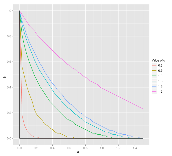
Figure 1: Strict stationarity zones for a GARCH(1,1) model with $\alpha$-stable innovation. The curves correspond, in decreasing order to $\alpha=2$, …, $\alpha=0.6$.

4 When the innovation process converges in distribution to a stable distribution

In this section, for clarity purpose, we will enunciate the results for a GARCH$(p,q)$ model (Model (1.2)). The same results could be obtained for a more general model but at the cost of some technical assumptions on the function $g$. We write a different version of Model (1.2) with an innovation process $(\eta_{nt})$ which now depends on $n$. We have,

$$\left\{\begin{aligned} \epsilon_{nt}&=\sigma_{nt}\eta_{nt}\\ \sigma_{nt}^{2}&=\omega_{0}+\sum_{i=1}^{q}a_{0i}\epsilon_{nt-i}^{2}+\sum_{j=1}^{p}b_{0j}\sigma_{nt-j}^{2},\quad\forall t\in\mathbb{Z},\ \forall n\in\mathbb{N},\end{aligned}\right.$$ (4.1)

where the process $(\eta_{nt})_{t}$ is iid with p.d.f. $f_{n}$ and converges in distribution toward a stable variable with parameter $\psi_{0}=(\alpha_{0},\beta_{0},\mu_{0})^{\prime}$. This assumption will be made explicit below. As in Section 3, the parameter $\gamma_{0}$ is omitted and fixed to 1 for identifiability reasons. The true parameter of the model is $\tau_{0}=\left(\theta_{0}^{\prime},\psi_{0}^{\prime}\right)^{\prime}$, where $\theta_{0}=\left(\omega_{0},a_{01},\ldots,a_{0q},b_{01},\ldots,b_{0p}\right)^{\prime}$ belongs to a parameter space $\Theta\subset(0,+\infty)\times\left[0,+\infty\right)^{p+q}$. The parameter $\tau_{0}$ belongs to $\Gamma=\Theta\times A\times B\times C$, with $A,B,C$ as in Section 3. Let the polynomials $\mathcal{A}_{\theta}(z)=\sum_{i=1}^{q}a_{i}z^{i}$ and $\mathcal{B}_{\theta}(z)=1-\sum_{j=1}^{p}b_{j}z^{j}$ where $\theta=(\omega,a_{1},\ldots,a_{q},b_{1},\ldots,b_{p})^{\prime}$. For $\theta$ such that $\sum_{j=1}^{p}b_{j}<1$ and $b_{j}\geq 0$ for $j\in\left\{1,\ldots,p\right\}$, define the function $\sigma_{nt}^{2}(\theta)=\frac{\omega}{\mathcal{B}_{\theta}(1)}+\mathcal{B}_{\theta}^{-1}(L)\mathcal{A}_{\theta}(L)\epsilon_{nt}^{2}$, where $L$ denotes the lag operator.

We suppose that the process $(\eta_{nt})_{t}$ is iid for every $n\in\mathbb{N}$, but we need a stronger assumption. Define for $t\in\mathbb{Z}$, $\mathcal{F}_{t}=\sigma\left(\cup_{n_{\in}\mathbb{N}}\mathcal{F}_{nt}\right)$, where $\mathcal{F}_{nt}=\sigma\left\{\eta_{nu};u\leq t-1\right\}$ and suppose that for any $t\in\mathbb{Z}$ and for any $n\in\mathbb{N}$, $\eta_{nt}$ is independent of $\mathcal{F}_{t}$.

We define a pseudo maximum likelihood estimator. The density of $(\eta_{nt})_{t}$ is not specified but we suppose the convergence of this process to the stable distribution with p.d.f. $f(.,\psi_{0})$, where $\psi_{0}$ is an unknown parameter. We use this density to build a pseudo MLE. We have for $\tau\in\Gamma$,

$$\tilde{I}_{n}(\tau)=\frac{1}{n}\sum_{t=1}^{n}\tilde{l}_{nt}(\tau)\quad\text{with}\quad\tilde{l}_{nt}(\tau)=\log\tilde{\sigma}_{nt}(\theta)-\log f\left(\frac{\epsilon_{nt}}{\tilde{\sigma}_{nt}(\theta)},\psi\right),$$

where the $(\tilde{\sigma}_{nt}(\theta))_{t}$ are recursively defined using some initial values. We define

$$\tau_{n}=\underset{\tau\in\Gamma}{\text{argmin}}\ \tilde{I}_{n}(\tau).$$ (4.2)

We have kept the same notations as in the previous section because all the involved quantities are defined in the same way and play the same role. The objects of this section simply display an additional $n$ subscript.

We define $\gamma_{n}$ as the top Lyapunov exponent associated to Model (4.1) and $\gamma$ as the top Lyapunov exponent associated to the model

$$\left\{\begin{aligned} \epsilon_{t}&=\sigma_{t}\eta_{t}\\ \sigma_{t}^{2}&=\omega_{0}+\sum_{i=1}^{q}a_{0i}\epsilon_{t-i}^{2}+\sum_{j=1}^{p}b_{0j}\sigma_{t-j}^{2},\quad\forall t\in\mathbb{Z},\end{aligned}\right.$$ (4.3)

with $\eta_{t}\sim S(\psi_{0})$. The top Lyapunov exponent will be more precisely defined in Section 7.

1. $\tau_{0}\in\Gamma$ and $\Gamma$ is a compact.

2. $\gamma<0$ and $\forall\theta\in\Theta,\ \sum_{j=1}^{p}b_{j}<1$.

3. There exists $\delta>1$ such that for any $n\in\mathbb{N}$, $E|\eta_{nt}|^{\delta}<+\infty$ and $\underset{x\in\mathbb{R}}{\sup}\ (1+|x|)^{\delta}|f_{n}(x)-f(x,\psi_{0})|\rightarrow 0$.

4. If $p>0$, $\mathcal{A}_{\theta_{0}}(z)$ and $\mathcal{B}_{\theta_{0}}(z)$ have no common roots, $\mathcal{A}_{\theta_{0}}(1)\neq 0$ and $a_{0q}+b_{0p}\neq 0$.

5. We have $\underset{n\in\mathbb{N}}{\sup}\ \alpha_{\epsilon_{n}}(h)\leq K\rho^{h}$, where $\alpha_{\epsilon_{n}}(h)$ for $h\in\mathbb{N}$ is the strong mixing coefficient of the process $(\epsilon_{nt})_{t}$.

6. $\tau_{0}\in\stackrel{{\scriptstyle\circ}}{{\Gamma}}$, where $\stackrel{{\scriptstyle\circ}}{{\Gamma}}$ denotes the interior of $\Gamma$.

Theorem 4.1.

Under Assumptions B1-B5, the estimator $\tau_{n}$ is consistent,

$$\tau_{n}\underset{n\rightarrow+\infty}{\longrightarrow}\tau_{0},\ a.s.$$ (4.4)

If, in addition B6 holds,

$$\sqrt{n}(\tau_{n}-\tau_{0})\stackrel{{\scriptstyle\mathcal{L}}}{{\rightarrow}}\mathcal{N}\left(0,J^{-1}\right),$$ (4.5)

with $J=E\left[\frac{\partial^{2}l_{t}(\tau_{0})}{\partial\tau\partial\tau^{\prime}}\right]=E\left[\frac{\partial l_{t}}{\partial\tau}(\tau_{0})\frac{\partial l_{t}}{\partial\tau^{\prime}}(\tau_{0})\right]$, where ${l}_{t}(\tau)$ is defined in the proofs.

Remark 4.1.

The variance-covariance matrix in Theorem 4.1 is the same as in Theorem 3.1. There is asymptotically no cost for not specifying the true distribution of the innovation and instead assuming that the process converges in distribution to a stable law.

Remark 4.2.

The required assumptions for this result are very mild, B1, B2, B4 and B6 are also needed for the classical Gaussian QML. Assumption B3 is specific to the problem and is verified in the case described hereafter where the innovation can be written as the sum of an iid process,

$$\eta_{nt}=\frac{1}{k_{n}^{1/\alpha}}\sum_{i=1}^{k_{n}}\nu_{it},$$

where for any $t\in\mathbb{Z}$, $(\nu_{it})_{i}$ is iid and where $(k_{n})_{n}$ is an increasing sequence of integers and with $\alpha\in(1,2)$ such that there exist $\ K_{1}$ and $K_{2}$ such that

$$\mathbb{P}\left[\nu_{1t}>x\right] \sim K_{1}x^{-\alpha},\ \mbox{when}\ x\rightarrow+\infty,$$

$$\mathbb{P}\left[\nu_{1t}<x\right] \sim K_{2}x^{-\alpha},\ \mbox{when}\ x\rightarrow-\infty,$$

then if the density of $\nu_{it}$ satisfies the assumptions of Theorems 2.2 and 2.3, the Assumption B3 is verified by Theorem 2.3.

Remark 4.3.

In the Gaussian QML case, the asymptotic inverse variance-covariance matrix $J$ depends on the unobserved distribution of the process $(\eta_{t})_{t}$. Here the matrix $J$ depends on the limit in distribution of the innovation process $(\eta_{nt})_{t}$. We can define an estimator for the matrix $J$, based on the process $(\epsilon_{nt})_{t}$ and prove that this estimator is consistent.

Remark 4.4.

About Assumption B5, for each value of $n$, the fact that there exist constants $K$ and $\rho$ such that $\alpha_{\epsilon_{n}}(h)\leq K\rho^{h}$ has been proved by Boussama (1998). We only assume that this is also true for $\underset{n\in\mathbb{N}}{\sup}\ \alpha_{\epsilon_{n}}(h)$.

Theorem 4.2.

Define $J_{n}=\frac{1}{n}\sum_{t=1}^{n}\frac{\partial^{2}\tilde{l}_{nt}}{\partial\tau\partial\tau^{\prime}}(\tau_{n})$. With the assumptions of Theorem 4.1, we have

$$J_{n}\underset{n\rightarrow+\infty}{\longrightarrow}J,\quad\mbox{a.s.}$$ (4.6)

5 Numerical experiments

In this section, we describe a simulation experiment which aims at studying the behavior of the pseudo MLE for finite samples, and for an innovation process whose distribution is close to a stable distribution. We use the algorithm of Chambers et al. (1976) to simulate stable processes and Proposition 2.1 to compute the stable density.

We want to verify that even if the model is misspecified, that is if we use a stable MLE when the true distribution of the innovation process is not stable, the GARCH coefficients are still correctly estimated. We use a Student distribution with degree of freedom $\alpha$ (which by Theorem 2.1 is in the domain of attraction of a stable law of parameter $\alpha$) to build an innovation process of the form

$$\eta_{t}^{(K)}=\frac{1}{K^{1/\alpha}}\sum_{k=1}^{K}\nu_{k,t},\quad\mbox{with}\quad(\nu_{k,t})_{k}\stackrel{{\scriptstyle iid}}{{\sim}}t_{\alpha}.$$

Using the results of Section 2, we obtain that, when $K$ tends to infinity, $\eta_{t}^{(K)}$ converges in distribution toward an alpha stable law. The problem is that, for identifiability reason, the parameter $\gamma$ of the stable distribution cannot be estimated and has to be fixed to $1$. When $K=+\infty$, the process $\left(\eta_{t}^{(+\infty)}\right)_{t}$ is alpha stable with parameter $\psi=\left(\alpha,\beta,\mu,\gamma\right)^{\prime}$. The parameter $\psi$ depends on the degree of freedom of the Student process $(\nu_{k,t})_{k}$ and can be calculated. For a generic case, we have $\gamma\neq 1$. If we estimate a GARCH model with innovation process $\left(\eta_{t}^{(+\infty)}\right)_{t}$ using a stable pseudo MLE method, we would obtain estimates of the parameters of the same model but written under a different identifiability assumption. For example, if we aim to estimate the model

$$\left\{\begin{aligned} \epsilon_{t}&=\sigma_{t}\eta_{t}^{(+\infty)}\\ \sigma_{t}^{2}&=\omega_{0}+a_{0}\epsilon_{t-1}^{2}+b_{0}\sigma_{t-1}^{2},\end{aligned}\right.$$

the stable pseudo MLE defined in the previous sections will converge toward $\theta_{0}^{*}=\left(\frac{\omega_{0}}{\gamma^{2}},\frac{a_{0}}{\gamma^{2}},b_{0}\right)^{\prime}$, see Francq et al. (2011) for more details on reparametrization of GARCH models. Note that the estimation of the “GARCH” parameter $b_{0}$ is not affected by the identification problem. In order to compare estimates of the same quantity, it is thus important that the model is similarly identified for each value of $K$. Thereafter, we use the following identifiability condition.

• If the innovation process $(\eta_{t})_{t}$ is stable, then it is stable with parameter $\gamma_{0}=1$ (we recall that, if $X$ is stable with parameter $\gamma=\gamma_{0}>0$ then $\frac{X}{\gamma_{0}}$ is stable with parameter $\gamma=1$).

• It the innovation process $(\eta_{t})_{t}$ is not stable, we require that, among the family of stable distributions, the closest distribution to the distribution of $(\eta_{t})_{t}$ in the sense of the Kulback-Leibler distance is stable with parameter $\gamma_{0}=1$.

Thus, for each $K$, we estimate the quantity $j_{K}$, defined such that the innovation process defined by $\eta_{t,K}=\frac{1}{j_{K}K^{1/\alpha}}\sum_{k=1}^{K}\nu_{k,t}$ satisfies the identifiability assumption. It is important to note that if we use another normalizing constant than $j_{K}$, the results of the estimation by stable pseudo ML are as efficient as in the case where we use $j_{K}$, the model is simply written under a different identifiability condition.

We generated 1000 samples of size $n=1000$ for different values of $K$ ($K=500,\ K=1000,\ K=10000,\ K=100000$ and $K=\infty$) of the following model and estimate its parameters by stable MLE (or pseudo MLE).

$$\left\{\begin{aligned} \epsilon_{t}&=\sigma_{t}\eta_{t,K}\\ \sigma_{t}^{2}&=0.01+0.02\epsilon_{t-1}^{2}+0.7\sigma_{t-1}^{2}\\ \eta_{t,K}&=\frac{1}{j_{K}K^{1/\alpha}}\sum_{k=1}^{K}\nu_{k,t}.\end{aligned}\right.$$ (5.1)

We can summarize the simulation scheme with the following steps. For a parameter $\theta_{0}$, for $K>0$ and for a student distribution of degree $\alpha$,

• Step 1: we simulate $1000$ samples of the variable $\left(\frac{1}{K^{1/\alpha}}\sum_{k=1}^{K}\nu_{k,t}\right)_{t}$, then we fit a stable distribution on each sample. For each sample $s$, we denote by $\psi_{s}=\left(\alpha_{s},\beta_{s},\mu_{s},\gamma_{s}\right)^{\prime}$ the results of this estimation.

• Step 2: we compute $j_{K}=\frac{1}{1000}\sum_{s=1}^{1000}\gamma_{s}$.

• Step 3: we draw $1000$ samples of Model (5.1).

• Step 4: for each sample $s$, we estimate $\tau_{n}^{(s)}=\left(\theta_{n}^{(s)^{\prime}},\psi_{n}{(s)^{\prime}}\right)^{\prime}$ by stable PMLE.

The results of these estimations are presented in Table 1. For each of the six parameters (three for the GARCH dynamic and three for the stable distribution), we give the quotient of the Root Mean Squared Errors (RMSE) of the corrected stable pseudo MLE and of the RMSE of the MLE, corresponding to the case $K=\infty$. This statistic is given by $Q_{i}^{K}=\frac{RMSE_{i}^{K=+\infty}}{RMSE_{i}^{K=K}}$ where the RMSE for $K$ can be obtained by, for $i\in\left\{1,\cdots,6\right\},\ RMSE_{i}^{K}=\frac{1}{1000}\sum_{s=1}^{1000}\left(\theta_{n,i}^{(s)}-\theta_{0,i}\right)^{2}$. The greater $Q_{i}$ is, the better the stable pseudo MLE is with respect to the MLE. In this simulation framework, we do not compare different methods of estimation. We use the same method but applied to different data generating processes. Table 1 shows that, concerning parameters $\omega$, $a$, $b$ and $\alpha$, the $(Q_{i})_{i\in\{1,\cdots,4\}}$ increase with $K$. For large values of $K$, the RMSE of the misspecified model is quite close to the RMSE of the asymptotic case, i.e. the well specified case. Table 1 also indicates that the result of the simulation for parameters $\beta$ and $\delta$ are more surprising. Indeed, the RMSE of the estimation of the asymmetry parameter $\beta$ is smaller when $K$ is small. But a good estimation of the parameter $\beta$ is not of much information if the parameter $\alpha$ is not well estimated. Finally, for large values of $K$, we find that our estimator is not much affected by the specification error on the density used to compute the likelihood.

	$\alpha=1.6$						$\alpha=1.4$
$K$	10	50	500	1000	10000	100000	10	50	500	1000	10000	100000
$w$	0.34	0.59	0.79	0.66	0.89	0.86	0.56	0.68	0.80	0.83	0.78	0.91
$a$	0.12	0.24	0.50	0.54	0.82	0.83	0.35	0.61	0.85	0.74	0.81	0.97
$b$	0.42	0.61	0.76	0.76	0.94	0.99	0.76	0.92	0.97	0.93	0.94	0.97
$\alpha$	0.17	0.31	0.58	0.70	0.91	1.03	0.57	0.84	0.93	0.94	0.95	0.96
$\beta$	2.45	1.45	1.27	1.22	1.05	1.01	1.29	0.92	0.84	1.12	0.86	1.04
$\delta$	1.26	0.96	0.96	0.87	0.89	0.86	1.07	0.96	0.90	1.09	0.90	0.93

Table 1: Ratio of RMSE for the parameters of the model for several values of $K$ and $\alpha$.

6 Application to financial data

In this section, we consider the daily returns of several indices and currency rates, namely the EURUSD, JPYUSD, DJA, DJI, DJT, DJU, CAC, FTSE, NIKKEI, DAX, S&P50 and the SMI. A GARCH(1,1) model with stable innovations is estimated on each of these series. The samples extend from January 1, 2008 to December 31, 2010. The estimated $\alpha$’s are lower for the period before 2008 so we only kept three years of data. Table 2 shows the results of these estimations with the standard deviation in parenthesis. We can see that even if the GARCH modeling explain a fraction of the leptokurticity of the series, the residuals still possess heavy tails since in most cases $\alpha$ is around 1.8 and thus different from 2 (except for the NIKKEI). When $\alpha=2$, the parameter $\beta$ cannot be identified.

Index	$\omega\times 10^{5}$		$a\times 10^{2}$		$b$		$\alpha$		$\beta$		$\mu$
EURUSD	0.133	( 0.047)	4.120	( 0.720)	0.877	( 0.025)	1.900	( 0.020)	-0.007	( 0.480)	-0.007	( 0.075)
JPYUSD	0.578	( 0.270)	3.370	( 0.770)	0.667	( 0.130)	1.780	( 0.037)	-0.148	( 0.190)	-0.137	( 0.062)
INRUSD	0.042	( 0.016)	2.300	( 0.630)	0.912	( 0.024)	1.820	( 0.077)	0.242	( 0.230)	-0.016	( 0.067)
DJA	0.050	( 0.044)	4.610	( 0.540)	0.895	( 0.014)	1.820	( 0.110)	-0.039	( 0.280)	0.028	( 0.071)
DJI	0.046	( 0.038)	4.670	( 0.400)	0.893	( 0.011)	1.840	( 0.083)	-0.501	( 0.270)	0.114	( 0.071)
DJT	0.071	( 0.070)	3.820	( 0.560)	0.916	( 0.014)	1.880	( 0.087)	-0.060	( 0.330)	0.060	( 0.067)
DJU	0.095	( 0.045)	4.690	( 0.700)	0.887	( 0.018)	1.910	( 0.068)	-0.296	( 0.360)	0.040	( 0.064)
CAC40	0.221	( 0.092)	2.970	( 0.550)	0.914	( 0.016)	1.880	( 0.072)	-0.220	( 0.210)	-0.010	( 0.058)
FTSE	0.156	( 0.067)	3.660	( 0.610)	0.898	( 0.019)	1.820	( 0.050)	-0.222	( 0.230)	0.059	( 0.060)
NIKKEI	0.376	( 0.140)	5.700	( 0.490)	0.863	( 0.021)	2.000	( 0.090)	NA	( NA)	-0.021	( 0.053)
DAX	0.136	( 0.051)	2.830	( 0.510)	0.922	( 0.014)	1.860	( 0.079)	-0.252	( 0.270)	0.034	( 0.065)
S&P500	0.909	( 0.250)	3.870	( 0.780)	0.766	( 0.055)	1.770	( 0.057)	-0.162	( 0.180)	0.103	( 0.062)
SMI	0.112	( 0.049)	4.850	( 0.470)	0.876	( 0.015)	1.850	( 0.077)	-0.255	( 0.250)	0.028	( 0.064)

Table 2: Estimation of a GARCH(1,1), standard errors in parenthesis.

These estimations can be used to compute Value-at-Risk (VaR). If $\epsilon_{t}$ is the return of the series, the VaR with coverage probability $p$ at time $t$ is defined as the quantity $\mbox{VaR}_{t}(p)$ satisfying

$$\mathbb{P}_{t}[\epsilon_{t}\leq\mbox{VaR}_{t}(p)]=p,$$

where $\mathbb{P}_{t}$ is the probability measure conditionally to the time $t-1$ information set. Using a conditionally heteroscedastic model with stable innovation, if $\tau_{n}=\left(\theta_{n}^{\prime},\psi_{n}^{\prime}\right)^{\prime}$ is the MLE (or pseudo MLE if the innovation is not stable but assumed to be close to a stable distribution), we have

$$\mbox{VaR}_{t}(p)=\tilde{\sigma}_{t-1}(\theta_{n})F^{\leftarrow}(p,\psi_{n}),$$

where $F^{\leftarrow}(.,\psi)$ is the quantile function of a stable distribution of parameter $\psi$ (with $\gamma=1$). We compare this stable VaR to the VaR computed using a GARCH(1,1) model, estimated with the Gaussian QMLE. We compute a Gaussian QMLE on the indices used in Table 2 and obtain the Gaussian counterparts of the parameters in this table.

Then we compute the Gaussian VaR and the stable VaR on an outsample data set (from January 1, 2011 to January 31, 2012). We give the results for the VaR of level $1\%$ and $5\%$ in Table 3.

Index	Level=0.01		Level=0.05
	Stable	Gaussian	Stable	Gaussian
EURUSD	0.0108	0.0180	0.0755	0.0791
JPYUSD	0.0035	0.0035	0.0177	0.0213
INRUSD	0.0106	0.0142	0.0426	0.0355
DJA	0.0221	0.0221	0.0551	0.0515
DJI	0.0147	0.0221	0.0551	0.0588
DJT	0.0294	0.0331	0.0588	0.0478
DJU	0.0110	0.0110	0.0551	0.0588
CAC40	0.0108	0.0179	0.0645	0.0717
FTSE	0.0037	0.0110	0.0625	0.0662
NIKKEI	0.0114	0.0114	0.0342	0.0342
DAX	0.0072	0.0143	0.0717	0.0789
S&P500	0.0074	0.0221	0.0699	0.0588
SMI	0.0109	0.0181	0.0688	0.0688
Mean	0.0118	0.0168	0.0563	0.0563

Table 3: Frequency of hits for the Gaussian VaR and the stable VaR

The two methods give very close results for $p=0.05$, but the Gaussian method seems unable to explain the extremes of the distribution and the stable VaR seems to give better results for $p=0.01$. In this case and for almost every index, the Gaussian VaR is underestimated. There are too many hits in the sample. We can conclude that the residuals of the GARCH model estimated by Gaussian QMLE are too leptokurtic to be explained by a Gaussian distribution. To conclude, the stable distribution seems to do a better job to explain the tails of the studied financial series.

7 Proofs

Throughout the proofs and the paper, we denote by $K$ and $\rho$ generic constants whose values $K>0$ and $0<\rho<1$ can vary from line to line.

7.1 Proof of the consistency in Theorem 3.1

Let $I_{n}$ (resp. $l_{t}$) be the equivalent of $\tilde{I}_{n}$ (resp. $\tilde{l}_{t}$) when an infinite past is known,

$${I}_{n}(\tau)=\frac{1}{n}\sum_{t=1}^{n}{l}_{t}(\tau)\quad\text{with}\quad{l}_{t}(\tau)=\frac{1}{2}\log{\sigma}_{t}^{2}(\theta)-\log f\left(\frac{\epsilon_{t}}{{\sigma}_{t}(\theta)},\psi\right).$$

We first prove that the initial values are asymptotically negligible, that is

$$\underset{n\rightarrow+\infty}{\lim}\ \underset{\tau\in\Gamma}{\sup}\ \left|I_{n}(\tau)-\tilde{I}_{n}(\tau)\right|=0\quad\text{a.s.}$$ (7.1)

We have,

$$\underset{\tau\in\Gamma}{\sup}\ \left|I_{n}(\tau)-\tilde{I}_{n}(\tau)\right|\leq\frac{1}{n}\sum_{t=1}^{n}\underset{\tau\in\Gamma}{\sup}\ \left|\frac{1}{2}\log\frac{\sigma_{t}^{2}(\theta)}{\tilde{\sigma}_{t}^{2}(\theta)}+\log\frac{f(\tilde{\eta}_{t}(\theta),\psi)}{f(\eta_{t}(\theta),\psi)}\right|,$$

where $\tilde{\eta}_{t}(\theta)=\frac{\epsilon_{t}}{\tilde{\sigma}_{t}(\theta)}$ and ${\eta}_{t}(\theta)=\frac{\epsilon_{t}}{{\sigma}_{t}(\theta)}$.

The function $f$ is infinitely differentiable with respect to $x$, therefore, for $\tau=(\theta^{\prime},\psi^{\prime})^{\prime}\in\Gamma$, we have

$$\left|\log f(\tilde{\eta}_{t}(\theta),\psi)-\log f(\eta_{t}(\theta),\psi)\right|<\underset{x\in\mathbb{R}}{\sup}\ \left|\frac{f^{\prime}(x,\psi)}{f(x,\psi)}\right|\left|\tilde{\eta}_{t}(\theta)-\eta_{t}(\theta)\right|.$$

Next, using the asymptotic expansion (2.6)-(2.7), we obtain that $\frac{f^{\prime}(x,\psi)}{f(x,\psi)}$ tends to 0, when $|x|$ tends to infinity and thus that $x\mapsto\frac{f^{\prime}(x,\psi)}{f(x,\psi)}$ is bounded on $\mathbb{R}$. This can be obtained since for any $\psi\in A\times B\times C$, the support of the function $x\mapsto f(x,\psi)$ is $\mathbb{R}$. Under Assumption A4, we obtain $\underset{\tau\in\Gamma}{\sup}\ \underset{x\in\mathbb{R}}{\sup}\ \left|\frac{f^{\prime}(x,\psi)}{f(x,\psi)}\right|<\infty$. Using Assumption A1 and A2, it can be seen that $\underset{\tau\in\Gamma}{\sup}\ \left|{\eta}_{t}(\theta)-\eta_{t}(\theta)\right|<K|\epsilon_{t}|$ and $\underset{\tau\in\Gamma}{\sup}\ \left|\tilde{\sigma}_{t}(\theta)-\sigma_{t}(\theta)\right|<K|\epsilon_{t}|\rho^{t}$. Thus we have $\underset{\tau\in\Gamma}{\sup}\ |\log f(\tilde{\eta}_{t}(\theta),\tau)-\log f(\eta_{t}(\theta),\tau)|<K|\epsilon_{t}|\rho^{t}$ and finally

$$\underset{\tau\in\Gamma}{\sup}\ \left|I_{n}(\tau)-\tilde{I}_{n}(\tau)\right|<\frac{1}{n}\sum_{t=1}^{n}K|\epsilon_{t}|\rho^{t}.$$

In view of the Markov inequality, the Borel-Cantelli Lemma, the existence of a moment of order $s$ for the processus $(\epsilon_{t})_{t}$ (Assumption A5) and Assumption A ‣ 3, we obtain that $|\epsilon_{t}|\rho^{t}$ converges to 0 almost surely when $t$ tends to infinity. Then, using the Cesàro Lemma, we obtain (7.1).

We now prove that $El_{t}(\tau)>El_{t}(\tau_{0})$, for $\tau\neq\tau_{0}$.

$$El_{t}(\tau)-El_{t}(\tau_{0}) =E\left[\log\frac{\sigma_{t}(\theta_{0})}{\sigma_{t}(\theta)}\frac{f(\eta_{t}(\theta),\psi)}{f(\eta_{t},\psi_{0})}\right]$$

$$\leq E\left[\frac{\sigma_{t}(\theta_{0})}{\sigma_{t}(\theta)}\frac{f(\eta_{t}(\theta),\psi)}{f(\eta_{t},\psi_{0})}\right]-1$$

$$=E\left[E\left[\frac{\sigma_{t}(\theta_{0})}{\sigma_{t}(\theta)}\frac{f(\frac{\sigma_{t}(\theta_{0})}{\sigma_{t}(\theta)}\eta_{t},\psi)}{f(\eta_{t},\psi_{0})}|\mathcal{G}_{t}\right]\right]-1$$

$$=0.$$

To obtain the last equality, we used the fact that $\frac{\sigma_{t}(\theta_{0})}{\sigma_{t}(\theta)}$ is in $\mathcal{G}_{t}=\sigma\left\{\eta_{u};\ u\leq t-1\right\}$.

Now, we show that, if $El_{t}(\tau)=El_{t}(\tau_{0})$, then $\tau=\tau_{0}$ a.s. We have $\frac{\sigma_{t}(\theta_{0})}{\sigma_{t}(\theta)}\frac{f(\frac{\sigma_{t}(\theta_{0})}{\sigma_{t}(\theta)}\eta_{t},\psi)}{f(\eta_{t},\psi_{0})}=1$ a.s. Let $a_{t-1}=\frac{\sigma_{t}(\theta_{0})}{\sigma_{t}(\theta)}$. The variable $(\eta_{t})_{t}$ has a Lebesgue density, this yields

$$\forall x\in\mathbb{R},\ a_{t-1}f(a_{t-1}x,\psi)=f(x,\psi_{0})\quad a.s.$$ (7.2)

We define $X$ as a stable variable with parameters $\psi_{0}$, $X\sim S(\psi_{0})$, and $Y=a_{t-1}X$. Then, using (7.2) we show that the pdf of $Y$ conditionally to $\mathcal{G}_{t}$ is $f(x,\psi)$, thus $Y\sim S(\psi)$. Now, for $u\in\mathbb{R}$, we write the characteristic function of $Y$ and obtain

$$E\left[e^{iuY}|\mathcal{G}_{t}\right] =E\left[e^{iua_{t-1}X}|\mathcal{G}_{t}\right],$$

that is $\varphi_{\psi}(u)=\varphi_{\psi_{0}}(a_{t-1}u)$. Applying the modula to the previous equation yields

$$\forall u\in\mathbb{R},\ \exp\left\{-|u|^{\alpha}\right\}=\exp\left\{-|a_{t-1}u|^{\alpha_{0}}\right\}.$$

Therefore we have $\alpha=\alpha_{0}$ and we easily obtain $\beta=\beta_{0}$ and $\mu=\mu_{0}$. We also obtain $a_{t-1}=1$ almost surely and we deduce with Assumption A3 that $\theta=\theta_{0}$ a.s.

Now, for $\tau\in\Gamma$, let $V_{k}(\tau)$ be the open ball with center $\tau$ and radius $1/k$, using (7.1), it follows that

$$\text{liminf}\ \underset{\tau^{*}\in V_{k}(\tau)\cap\Gamma}{\inf}\tilde{I}_{n}(\tau^{*})=\text{liminf}\ \underset{\tau^{*}\in V_{k}(\tau)\cap\Gamma}{\inf}{I}_{n}(\tau^{*}),$$ (7.3)

The ergodic theorem yields $\text{liminf}\ \underset{\tau^{*}\in V_{k}(\tau)\cap\Gamma}{\inf}{I}_{n}(\tau^{*})\geq E\left[\underset{\tau^{*}\in V_{k}(\tau)\cap\Gamma}{\inf}l_{t}(\tau^{*})\right]$. When $k\rightarrow+\infty$, then $E\left[\underset{\tau^{*}\in V_{k}(\tau)\cap\Gamma}{\inf}l_{t}(\tau^{*})\right]$ tends toward $E\left[l_{t}(\tau)\right]$. Therefore, we have

$$\forall\tau\neq\tau_{0},\ \exists V(\tau),\ \text{liminf}\ \underset{\tau^{*}\in V_{k}(\tau)\cap\Gamma}{\inf}\tilde{I}_{n}(\tau^{*})>El_{t}(\tau_{0}).$$

We conclude by a standard compactness argument, using Assumption A4 and obtain (3.2).

7.2 Proof of the asymptotic normality in Theorem 3.1

Lemma 7.1.

Under the assumptions of Theorem 3.1, we have

$$\sqrt{n}\frac{\partial I_{n}}{\partial\tau}(\tau_{0})\stackrel{{\scriptstyle\mathcal{L}}}{{\rightarrow}}\mathcal{N}(0,J).$$ (7.4)

Proof.

For $\lambda\in\mathbb{R}^{m+3}$, $n>0$ and $t>0$, let $\nu_{nt}=\frac{1}{\sqrt{n}}\lambda^{\prime}\frac{\partial l_{t}}{\partial\tau}(\tau_{0})$. We prove that $(\nu_{nt},\mathcal{G}_{t-1})$ is a martingale difference. We have, for $\tau=(\theta^{\prime},\psi^{\prime})^{\prime}\in\Gamma$

$$\frac{\partial l_{t}}{\partial\theta}(\tau) =\frac{1}{2}\phi_{t}(\theta)Z_{t}(\tau),$$ (7.5)

$$\frac{\partial l_{t}}{\partial\psi}(\tau) =-\frac{\partial\log f}{\partial\psi}(\eta_{t}(\theta),\psi),$$ (7.6)

with $Z_{t}(\tau)=1+\eta_{t}(\theta)\frac{f^{\prime}(\eta_{t}(\theta),\psi)}{f(\eta_{t}(\theta),\psi)}.$

Since $\sigma_{t}^{2}(\theta_{0})\in\mathcal{G}_{t}$, $\sigma_{t}(\theta_{0})$ and $\eta_{t}$ are independent and

$$E\left|\frac{\partial l_{t}}{\partial\theta}(\tau_{0})\right|=E\left|\phi_{t}(\theta_{0})\right|E\left|Z_{t}(_{a}u_{0})\right|.$$

The function $x\mapsto 1+x\frac{f^{\prime}(x,\psi_{0})}{f(x,\psi_{0})}$ is bounded, therefore we have $E\left|Z_{t}(\tau_{0})\right|<+\infty$. Moreover, with Assumption A6, we have $E\left|\phi_{t}(\theta_{0})\right|<+\infty$. With (2.8)-(2.10), we obtain $E\left|\nu_{nt}\right|<+\infty$.

Now, we have

$$E\left[\frac{\partial l_{t}}{\partial\theta}(\tau_{0})|\mathcal{G}_{t}\right]=\phi_{t}(\theta_{0})E\left[Z_{t}(\tau_{0})\right].$$

And,

$$E\left[Z_{t}(\tau_{0})\right]=1+\int_{\mathbb{R}}xf^{\prime}(x,\psi_{0})dx=0.$$

We infer $E\left[\frac{\partial l_{t}}{\partial\theta}(\tau_{0})\right]=0$. Now, we prove $E\left[\frac{\partial l_{t}}{\partial\alpha}(\tau_{0})|\mathcal{G}_{t}\right]=0$. Note that

$$E\left[\frac{\partial l_{t}}{\partial\alpha}(\tau_{0})|\mathcal{G}_{t}\right]=-\int_{\mathbb{R}}\frac{\partial f}{\partial\alpha}(x,\psi_{0})dx.$$

The function $x\mapsto f(x,\psi_{0})$ is integrable, therefore

$$\frac{\partial\varphi_{\psi_{0}}(u)}{\partial\alpha}=-\int_{\mathbb{R}}e^{iux}\frac{\partial f}{\partial\alpha}(x,\psi_{0})dx,\quad\text{and}\quad\frac{\partial\varphi_{\psi_{0}}(0)}{\partial\alpha}=E\left[\frac{\partial l_{t}}{\partial\alpha}(\tau_{0})\right].$$

We have, $\forall\alpha,\ \varphi_{\alpha,\beta_{0},\mu_{0},\gamma_{0}}(0)=0$, thus, $\frac{\partial\varphi_{\psi_{0}}}{\partial\alpha}(0)=0$. Using the same method for $\frac{\partial l_{t}}{\partial\beta}$, $\frac{\partial l_{t}}{\partial\mu}$ and $\frac{\partial l_{t}}{\partial\gamma}$ we obtain $E\left[\nu_{nt}|\mathcal{G}_{t}\right]=0$.

We now prove that the covariance matrix of the vector of derivatives of $l_{t}$ is finite, we have

$$E\left[\frac{\partial l_{t}}{\partial\theta}(\tau_{0})\frac{\partial l_{t}}{\partial\theta^{\prime}}(\tau_{0})\right]=\frac{1}{4}E\left[Z_{t}^{2}(\tau_{0})\right]E\left[\phi_{t}(\theta_{0})\phi_{t}^{\prime}(\theta_{0})\right],$$

with $E\left[Z_{t}^{2}(\tau_{0})\right]=1+2\int_{\mathbb{R}}xf^{\prime}(x,\psi_{0})dx+\int_{\mathbb{R}}x^{2}\frac{f^{{}^{\prime}2}(x,\psi_{0})}{f(x,\psi_{0})}dx$. From the asymptotic expansions in (2.6)-(2.10), we obtain $E\left[Z_{t}^{2}(\tau_{0})\right]<+\infty$, then by Assumption A6, it can be seen that $V\left[\frac{\partial l_{t}}{\partial\theta}(\tau_{0})\right]$ is finite.

Using the asymptotic expansion again, we have when $x\rightarrow\pm\infty$, for $\psi\in A\times B\times C$

$$\frac{\partial\log f}{\partial\alpha}(x,\psi)\sim K\log|x|,\ \frac{\partial\log f}{\partial\beta}(x,\psi)\sim K,\ \frac{\partial\log f}{\partial\mu}(x,\psi)\sim Kx^{-1},$$ (7.7)

therefore, for $(i,j)\in\left\{1,\cdots,3\right\}$, we have $E\left[\frac{\partial l_{t}}{\partial\psi_{i}}\frac{\partial l_{t}}{\partial\psi_{j}}\right]$ is finite. The very same reasoning applies for $E\left[\frac{\partial l_{t}}{\partial\psi}\frac{\partial l_{t}}{\partial\theta}\right]$ and we deduce $V\left[\frac{\partial l_{t}}{\partial\tau}\right]<+\infty$.

We now show that this matrix is positive-definite. Suppose that $(u^{\prime},v^{\prime})^{\prime}\in\mathbb{R}^{m+3}$ are such that $(u^{\prime},v^{\prime}).\frac{\partial l_{t}}{\partial\tau}(\tau_{0})=0$. We have

$$\left(1+\eta_{t}\frac{f^{\prime}(\eta_{t},\psi)}{f(\eta_{t},\psi)}\right)\frac{1}{2}u^{\prime}\phi_{t}(\theta_{0})=v^{\prime}\frac{\partial\log f}{\partial\psi}(\eta_{t},\psi).$$ (7.8)

Now, it can be seen that $\left(1+\eta_{t}\frac{f^{\prime}(\eta_{t},\psi)}{f(\eta_{t},\psi)}\right)\in\mathcal{G}_{t+1}$, $v^{\prime}\frac{\partial\log f}{\partial\psi}(\eta_{t},\psi)\in\mathcal{G}_{t+1}$ and $\frac{1}{2}u^{\prime}\phi_{t}(\theta_{0})\in\mathcal{G}_{t}$. Thus, we have $\frac{1}{2}u^{\prime}\phi_{t}(\theta_{0})=Q$ and

$$Q\left(1+\eta_{t}\frac{f^{\prime}(\eta_{t},\psi)}{f(\eta_{t},\psi)}\right)=v_{1}\frac{\partial\log f}{\partial\alpha}(\eta_{t},\alpha,\beta)+v_{2}\frac{\partial\log f}{\partial\beta}(\eta_{t},\alpha,\beta)+v_{3}\frac{\partial\log f}{\partial\mu},$$

with $v=(v_{1},v_{2},v_{3})$. We have when $x\rightarrow+\infty$, $x\frac{f^{\prime}(x,\alpha,\beta)}{f(x,\alpha,\beta)}\sim K$, then using Equation (7.7) and letting $x\rightarrow\infty$, we obtain $v_{1}=0$ and $\forall x\in\mathbb{R}$

$$Q\left(f(x,\psi)+xf^{\prime}(x,\psi)\right)=v_{2}\frac{\partial f}{\partial\beta}(x,\psi)+v_{3}\frac{\partial f}{\partial\mu}(x,\psi).$$

Now multiplying both sides of the previous equation by $e^{itx}$ and integrating on $\mathbb{R}$, we recognize the characteristic function of a stable distribution or its derivatives and obtain for $t\in\mathbb{R}$,

$$-Qt\frac{\partial\varphi_{\psi}(t)}{\partial t}=v_{2}\frac{\partial\varphi_{\psi}(t)}{\partial\beta}+v_{3}\frac{\partial\varphi_{\psi}(t)}{\partial\mu}.$$

Then, for $t>0$, it follows that

$$Q\left(\alpha t^{\alpha}-i\beta\tan\frac{\alpha\pi}{2}(\alpha t^{\alpha}-t)\right)=v_{2}i\tan\frac{\alpha\pi}{2}(t^{\alpha}-t)+v_{3}it.$$

Therefore, we have $Q=0$ and then $v_{2}=v_{3}=0$. Finally, with Assumption A8 we obtain $u=0_{m}$.

We have, if $(u^{\prime},v^{\prime})\ \frac{\partial l_{t}}{\partial\tau}(\tau_{0})=0$ then $(u^{\prime},v^{\prime})^{\prime}=0_{m+3}$ and the matrix $E\left[\frac{\partial l_{t}}{\partial\tau}(\tau_{0})\frac{\partial l_{t}}{\partial\tau^{\prime}}(\tau_{0})\right]$ is positive. Finally, using the central limit theorem for martingale differences and the Wold-Cramér Lemma we obtain (7.4) with $\Lambda=V\left[\frac{\partial l_{t}}{\partial\tau}\right]$. ∎

Lemma 7.2.

Under the assumptions of Theorem 3.1, for any compact subset $\Gamma^{*}$ in the interior of $\Gamma$, we have

$$E\left[\underset{\tau\in\Gamma^{*}}{\sup}\ \left|\frac{\partial^{3}l_{t}}{\partial\tau_{i}\tau_{j}\tau_{k}}(\tau)\right|\right]<+\infty.$$ (7.9)

Proof.

For ease of notation, the next equations are written without their argument $\tau=(\theta,\psi)\in\Gamma$. We have

$$\frac{\partial^{2}l_{t}}{\partial\theta_{i}\partial\theta_{j}} = \frac{1}{2}\left(\frac{1}{\sigma_{t}^{2}}\frac{\partial^{2}\sigma_{t}^{2}}{\partial\theta_{i}\theta_{j}}-\phi_{t,i}\phi_{t,j}\right)\left(1+\eta_{t}(\theta)\frac{\partial\log f}{\partial x}\right)$$

$$-\frac{1}{4}\phi_{t,i}\phi_{t,j}\eta_{t}(\theta)\left(\frac{\partial\log f}{\partial x}+\eta_{t}(\theta)\frac{\partial^{2}\log f}{\partial x^{2}}\right),$$

$$\frac{\partial^{2}l_{t}}{\partial\theta_{i}\partial\psi} = \frac{1}{2}\phi_{t,i}\eta_{t}(\theta)\frac{\partial^{2}\log f}{\partial x\partial\psi},$$ (7.11)

$$\frac{\partial^{3}l_{t}}{\partial\theta_{i}\partial\theta_{j}\partial\theta_{k}} = -\left(\phi_{t,i}\phi_{t,j,k}+\phi_{t,j}\phi_{t,i,k}+\phi_{t,k}\phi_{t,i,j}\right)\left(\frac{1}{2}+\frac{3}{4}\eta_{t}(\theta)\frac{\partial\log f}{\partial x}-\frac{1}{4}\eta_{t}^{2}(\theta)\frac{\partial^{2}\log f}{\partial x^{2}}\right)$$

$$+\phi_{t,i}\phi_{t,j}\phi_{t,k}\left(1+\frac{15}{8}\eta_{t}(\theta)\frac{\partial\log f}{\partial x}+\frac{9}{8}\eta_{t}^{2}(\theta)\frac{\partial^{2}\log f}{\partial x^{2}}+\frac{1}{4}\eta_{t}^{3}(\theta)\frac{\partial^{3}\log f}{\partial x^{3}}\right)$$

$$+\frac{1}{2}\phi_{t,i,j,k}\left(1+\eta_{t}(\theta)\frac{\partial\log f}{\partial x}\right),$$

We show that

$$E\ \underset{\tau\in\Gamma}{\sup}\left|\eta_{t}(\theta)\frac{\partial\log f}{\partial x}\left(\eta_{t}(\theta),\psi\right)\right|<\infty.$$ (7.12)

For any $\psi\in A\times B\times C$, the function $x\mapsto\left|x\frac{\partial\log f}{\partial x}(x,\psi)\right|$ is bounded. Then, the function $\psi\mapsto\underset{x}{\sup}\ \left|x\frac{\partial\log f}{\partial x}(x,\psi)\right|$ is continuous, thus since $A\times B\times C$ is a compact set, we obtain (7.12).

Using the same method for $\eta_{t}^{2}(\theta)\frac{\partial^{2}\log f}{\partial x^{2}}(\eta_{t}(\theta),\psi)$ and $\eta_{t}^{3}(\theta)\frac{\partial^{3}\log f}{\partial x^{3}}(\eta_{t}(\theta),\psi)$ and using Assumption A6 we obtain that, for any compact subset $\Gamma^{*}$ in the interior of $\Gamma$

$$E\left[\underset{\tau\in V}{\sup}\ \left|\frac{\partial^{3}l_{t}}{\partial\theta_{i}\theta_{j}\theta_{k}}(\tau)\right|\right]<+\infty.$$

With the same reasoning and other calculations, we obtain Equation  (7.9). ∎

Lemma 7.3.

Under the assumptions of Theorem 3.1, we have when $n\rightarrow+\infty$

$$\left\|\frac{1}{\sqrt{n}}\sum_{t=1}^{n}\left\{\frac{\partial l_{t}}{\partial\tau}(\tau_{0})-\frac{\partial\tilde{l}_{t}}{\partial\tau}(\tau_{0})\right\}\right\| \rightarrow 0,$$ (7.13)

$$\underset{\tau\in\Gamma}{\sup}\left\|\frac{1}{n}\sum_{t=1}^{n}\left\{\frac{\partial^{2}l_{t}}{\partial\tau\partial\tau^{\prime}}(\tau)-\frac{\partial^{2}\tilde{l}_{t}}{\partial\tau\tau^{\prime}}(\tau)\right\}\right\| \rightarrow 0.$$ (7.14)

Proof.

We have

$$\frac{\partial l_{t}}{\partial\theta}(\tau_{0})-\frac{\partial\tilde{l}_{t}}{\partial\theta}(\tau_{0}) =\frac{1}{2}\tilde{\phi}_{t}\tilde{Z}_{t}-\frac{1}{2}\phi_{t}Z_{t}$$

$$=\frac{1}{2}\left\{\tilde{\phi}_{t}\left(\tilde{Z}_{t}-Z_{t}\right)+Z_{t}\left(\tilde{\phi}_{t}-\phi_{t}\right)\right\}.$$ (7.15)

For $\psi\in A\times B\times C$, define the function $h$ as $h(x)=1+x\frac{\partial\log f}{\partial x}(x,\psi)$, we have $\tilde{Z}_{t}-Z_{t}=h\left(\tilde{\eta}_{t}\right)-h(\eta_{t})$. When $x\rightarrow\pm\infty$, we have $h^{\prime}(x)=O(x^{-1})$, therefore, with the mean value theorem, we have

$$\left|\tilde{Z}_{t}-Z_{t}\right|<K|\tilde{\eta}_{t}-\eta_{t}|<K|\epsilon_{t}|\left|\tilde{\sigma}_{t}^{2}-\sigma_{t}^{2}\right|.$$

On the other side, concerning the second term in  (7.15), we obtain

$$\left|\tilde{\phi}_{t}-\phi_{t}\right| <\frac{1}{\tilde{\sigma}_{t}^{2}}\left|\frac{\partial\tilde{\sigma}_{t}^{2}}{\partial\theta}-\frac{\partial{\sigma}_{t}^{2}}{\partial\theta}\right|+\frac{\partial{\sigma}_{t}^{2}}{\partial\theta}\left|\frac{1}{\tilde{\sigma}_{t}^{2}}-\frac{1}{{\sigma}_{t}^{2}}\right|$$

$$<K\left|\frac{\partial\tilde{\sigma}_{t}^{2}}{\partial\theta}-\frac{\partial{\sigma}_{t}^{2}}{\partial\theta}\right|+\frac{1}{{\sigma}_{t}^{2}}\frac{\partial{\sigma}_{t}^{2}}{\partial\theta}\left|\frac{\sigma_{t}^{2}}{\tilde{\sigma}_{t}^{2}}-1\right|.$$

Concerning the derivatives relative to the stable parameter $\psi$, it follows with the mean value theorem that

$$\left|\frac{\partial\log f}{\partial\alpha}(\tilde{\eta}_{t},\psi)-\frac{\partial\log f}{\partial\alpha}({\eta}_{t},\psi)\right|<\underset{x\in\mathbb{R}}{\sup}\left|\frac{\partial^{2}\log f}{\partial x\partial\alpha}(x,\psi)\right||\tilde{\eta}_{t}-\eta_{t}|.$$

The derivative of $\log f$ with respect to $\alpha$ and $x$ is bounded. Besides, we have

$$\left|\tilde{\eta}_{t}-\eta_{t}\right|=\left|\frac{\epsilon_{t}}{\tilde{\sigma}_{t}}-\frac{\epsilon_{t}}{{\sigma}_{t}}\right|<K|\epsilon_{t}|\left|\tilde{\sigma}_{t}^{2}-\sigma_{t}^{2}\right|.$$

We can apply the same method for the derivatives with respect to $\beta$ and $\mu$. Therefore, using Assumption A7, the Markov inequality, the Borel-Cantelli lemma and the Cesàro Lemma, we easily obtain (7.13).

Using (7.2), (7.11), the second part of Assumption A7 and the same techniques as before, we obtain (7.14). ∎

Proof of Theorem 3.1.

From the definition of the ML estimator $\tau_{n}$, we have $\frac{\partial\tilde{I}_{n}}{\partial\tau}(\tau_{n})=0$, writing a Taylor expansion, we infer

$$0=\frac{\partial\tilde{I}_{n}}{\partial\tau}(\tau_{n})=\frac{\partial\tilde{I}_{n}}{\partial\tau}(\tau_{0})+\frac{\partial^{2}\tilde{I}_{n}}{\partial\tau\partial\tau^{\prime}}(\tau^{*})(\tau_{n}-\tau_{0}),$$

where $\tau^{*}$ is between $\tau_{0}$ and $\tau_{n}$. Using another Taylor expansion, Lemma 7.2, the almost sure convergence of $\tau_{n}$ to $\tau_{0}$ and the ergodic theorem, we obtain

$$\frac{\partial^{2}I_{n}}{\partial\tau\partial\tau^{\prime}}(\tau^{*})\rightarrow E\left[\frac{\partial^{2}l_{t}}{\partial\tau\partial\tau^{\prime}}(\tau_{0})\right],\quad\mbox{a.s.}$$

Then, in view of Equations (7.5), (7.6), (7.2) and  (7.11), we obtain

$$E\left[\frac{\partial^{2}l_{t}}{\partial\tau\partial\tau^{\prime}}(\tau_{0})\right]=E\left[\frac{\partial l_{t}}{\partial\tau}(\tau_{0})\frac{\partial l_{t}}{\partial\tau^{\prime}}(\tau_{0})\right].$$

By Lemmas 7.1 and 7.3 we can conclude and obtain (3.3). ∎

7.3 Proof of the consistency in Theorem 4.1

Let $I_{n}$ (resp. $l_{nt}$) be the equivalent of $\tilde{I}_{n}$ (resp. $\tilde{l}_{nt}$) when an infinite past is known.

$$I_{n}(\tau)=\frac{1}{n}\sum_{t=1}^{n}l_{nt}(\tau),\ \mbox{with}\quad l_{nt}(\tau)=\frac{1}{2}\log\sigma_{nt}^{2}(\theta)-\log f\left(\frac{\epsilon_{nt}}{\sigma_{nt}(\theta)},\psi\right).$$

We also need to define the equivalent of these quantities when the processus $(\eta_{nt})_{t}$ is replaced by its limit in distribution $(\eta_{t})_{t}$. If $(\epsilon_{t})_{t}$ is the stationary ergodic solution of Model (4.3), we define $\sigma_{t}^{2}(\theta)=\frac{\omega}{\mathcal{B}_{\theta}(1)}+\mathcal{B}_{\theta}^{-1}(L)\mathcal{A}_{\theta}(L)\epsilon_{t}^{2}$ and $l_{t}(\tau)=\frac{1}{2}\log\sigma_{t}^{2}(\theta)-\log f\left(\frac{\epsilon_{t}}{\sigma_{t}(\theta)},\psi\right)$.

Assumption B3 can only be used for quantities which depend on a finite number of $(\eta_{nt})_{t}$. Therefore, we introduce $\sigma_{nt}^{2(m)}(\theta)$, a truncated version of $\sigma_{nt}^{2}(\theta)$. For that, we give a vector representation of the GARCH$(p,q)$ model as in Bougerol and Picard (1992),

$$\underline{z}_{nt}=\underline{b}_{nt}+A_{nt}\underline{z}_{nt-1},$$

where

$$\underline{b}_{nt}=\left(\begin{array}[]{c}\omega_{0}\eta_{nt}^{2}\\ 0\\ \vdots\\ \omega_{0}\\ 0\\ \vdots\\ \end{array}\right)\in\mathbb{R}^{p+q},\ \underline{z}_{nt}=\left(\begin{array}[]{c}\epsilon_{nt}^{2}\\ \vdots\\ \epsilon_{nt-q+1}^{2}\\ \sigma_{nt}^{2}\\ \vdots\\ \sigma_{nt-p+1}^{2}\\ \end{array}\right)\in\mathbb{R}^{p+q},$$

and

$$A_{nt}=\left(\begin{array}[]{cccccccccc}a_{01}\eta_{nt}^{2}&&\cdots&&a_{0q}\eta_{nt}^{2}&b_{01}\eta_{nt}^{2}&&\cdots&&b_{0p}\eta_{nt}^{2}\\ 1&0&\cdots&&0&0&&\cdots&&0\\ 0&1&\cdots&&0&0&&\cdots&&0\\ \vdots&\ddots&\ddots&&\vdots&\vdots&\ddots&\ddots&&\vdots\\ 0&&\cdots&1&0&0&&\cdots&0&0\\ a_{01}&&\cdots&&a_{0q}&b_{01}&&\cdots&&b_{0p}\\ 0&&\cdots&&0&1&0&\cdots&&0\\ 0&&\cdots&&0&0&1&\cdots&&0\\ \vdots&\ddots&\ddots&&\vdots&\vdots&\ddots&\ddots&&\cdots\\ 0&&\cdots&0&0&0&&\cdots&1&0\\ \end{array}\right).$$

We also define $\underline{z}_{t},\ \underline{b}_{t}$ and $A_{t}$, the counterparts of $\underline{z}_{nt},\ \underline{b}_{nt}$ and $A_{nt}$ where $\eta_{nt}$ is replaced by the iid sequence $(\eta_{t})_{t}$ defined in (4.3). Note that $\gamma_{n}$ is the top Lyapunov exponent associated to the sequence $(A_{nt})_{t\in\mathbb{Z}}$. Now, we prove that Assumption B2 implies that $\gamma_{n}$ is inferior to zero.

With Lemma 7.22 below, we obtain for any $n\in\mathbb{N}$,

$$\underline{z}_{nt}=\underline{b}_{nt}+\sum_{k=1}^{+\infty}A_{nt}A_{nt-1}\ldots A_{nt-k+1}\underline{b}_{nt-k}.$$ (7.16)

We define the truncated version of $\underline{z}_{nt}$. For any $m\in\mathbb{N}$,

$$\underline{z}_{nt}^{(m)}=\underline{b}_{nt}+\sum_{k=1}^{m}A_{nt}A_{nt-1}\ldots A_{nt-k+1}\underline{b}_{nt-k},\ \forall t\in\mathbb{Z},\ \forall n\in\mathbb{N}.$$ (7.17)

In particular, if $X(k)$ is the $k^{\mbox{th}}$ element of the vector $X$, we define a truncated version of $\sigma_{nt}^{2}$, that is

$$\underline{z}_{nt}^{(m)}(q+1)=\underline{b}_{nt}(q+1)+\left(\sum_{k=1}^{m}A_{nt}A_{nt-1}\ldots A_{nt-k+1}\underline{b}_{nt-k}\right)(q+1).$$ (7.18)

The quantity $\underline{z}_{nt}^{(m)}(q+1)$ depends only on $\left\{\eta_{nt-1},\ldots,\eta_{nt-m}\right\}$.

Then we define $\sigma_{nt}^{2(m)}(\theta)$ for any $\theta\in\Theta$. For this purpose, we introduce another vector representation of the model,

$$\underline{\sigma}_{nt}^{2}(\theta)=\underline{c}_{nt}(\theta)+B\underline{\sigma}_{nt-1}^{2}(\theta),$$

where

$$\underline{\sigma}_{nt}^{2}(\theta)=\left(\begin{array}[]{c}\sigma_{nt}^{2}(\theta)\\ \sigma_{nt-1}^{2}(\theta)\\ \vdots\\ \sigma_{nt-p+1}^{2}(\theta)\\ \end{array}\right),\;\underline{c}_{nt}(\theta)=\left(\begin{array}[]{c}\omega+\sum_{i=1}^{q}a_{i}\epsilon_{nt-i}^{2}\\ 0\\ \vdots\\ 0\\ \end{array}\right),\;B=\left(\begin{array}[]{cccc}b_{1}&b_{2}&\cdots&b_{p}\\ 1&0&\cdots&0\\ \vdots&&&\\ 0&\cdots&1&0\\ \end{array}\right).$$

By Assumption B2, we have $\underset{\theta\in\Theta}{\sup}\ \rho(B)<1$, where $\rho(B)$ is the spectral radius of the matrix $B$, and thus, for any $\theta\in\Theta$,

$$\underline{\sigma}_{nt}^{2}(\theta)=\sum_{k=0}^{+\infty}B^{k}\underline{c}_{nt-k}(\theta).$$ (7.19)

We define for $m\in\mathbb{N}$,

$$\sigma_{nt}^{2(m)}(\theta)=\sum_{k=0}^{m}B^{k}(1,1)\underline{c}_{nt-k}^{(m)}(\theta)(1),\ \mbox{with}\ \underline{c}_{nt}^{(m)}(\theta)(1)=\omega+\sum_{i=1}^{q}a_{i}\underline{z}_{nt-i}^{(m)}(q+1)\eta_{nt-i}^{2}.$$ (7.20)

As for $\underline{z}_{nt}^{(m)}(q+1)$, the quantity $\sigma_{nt}^{2(m)}(\theta)$ depends on a finite number of $\eta_{nt^{\prime}}$, but since every $\underline{z}_{nt-i}^{(m)}(q+1)$ depends on several $\eta_{nt^{\prime}}$, $\sigma_{nt}^{2(m)}(\theta)$ depends on more than $m$ variables $\eta_{nt^{\prime}}$. To be precise, $\sigma_{nt}^{2(m)}(\theta)$ depends on $\left\{\eta_{nt-1},\ldots,\eta_{nt-2m+q}\right\}$. Define also $l_{nt}^{(m)}(\tau)=\frac{1}{2}\log\sigma_{nt}^{2(m)}(\theta)-\log f\left(\frac{\epsilon_{nt}}{\sigma_{nt}^{2(m)}(\theta)},\psi\right)$.

Lemma 7.4.

Under the assumptions of Theorem 4.1, there exists $N\in\mathbb{N}$ such that

$$\forall n\geq N,\ \gamma_{n}<0.$$ (7.21)

Besides, there exist $k_{0}\in\mathbb{N}$ and $N\in\mathbb{N}$ such that

$$\chi^{\prime}=\underset{n\geq N}{\sup}\ E\left[\left\|A_{nk_{0}}A_{nk_{0}-1}\cdots A_{n1}\right\|^{s}\right]<1.$$ (7.22)

Proof of Lemma 7.22.

With Assumption B2, using the norm $\left\|A\right\|=\sum|a_{ij}|$, which is a multiplicative norm and with Lemma 2.3 in Francq and Zakoian (2010), we have the existence of $k_{0}\in\mathbb{N}$ and of $s>0$ such that

$$\chi=E\left[\left\|A_{k_{0}}A_{k_{0}-1}\cdots A_{1}\right\|^{s}\right]<1.$$

Now for $n\in\mathbb{N}$, writing $A_{nt}=A(\eta_{nt})$ to emphasize the fact that $A_{nt}$ only depends on $\eta_{nt}$, we have for $s>0$

$$E\left[\left\|A_{nk_{0}}A_{nk_{0}-1}\cdots A_{1n}\right\|^{s}\right]=\int_{\mathbb{R}^{k_{0}}}\left\|A(x_{1})\cdots A(x_{k_{0}})\right\|^{s}f_{n}(x_{1})\cdots f_{n}(x_{k_{0}})dx_{1}\cdots d{x_{k_{0}}}.$$

For $\varepsilon>0$, by Assumption B3, we have the existence of $N\in\mathbb{N}$, such that

$$\forall n\geq N,\ \forall x\in\mathbb{R},\ f_{n}(x)\leq G(x),\ \mbox{where}\ G(x)=f(x)+\frac{\varepsilon}{(1+|x|)^{\delta}}.$$

Then, the function $A$ is such that $\forall x\in\mathbb{R},\ 0<\|A(x)\|<Kx^{2}$ and therefore

$$\left\|A(x_{1})\cdots A(x_{k_{0}})\right\|^{s}f_{n}(x_{1})\cdots f_{n}(x_{k_{0}})\leq K\prod_{i=1}^{k_{0}}|x_{i}|^{2s}G(x_{i}),$$

Using the asymptotic expansion (2.6) and choosing $0<s<\min\left(\frac{\delta-1}{2},\frac{\alpha}{2}\right)$, we infer

$$\int_{\mathbb{R}^{k_{0}}}K\prod_{i=1}^{k_{0}}|x_{i}|^{2s}G(x_{i})\prod_{i=1}^{k_{0}}dx_{i}<+\infty,$$

Thus, since $f_{n}$ simply converges to $f(.,\psi_{0})$, using the dominated convergence theorem, we obtain

$$\underset{n\rightarrow+\infty}{\lim}\ E\left[\left\|A_{nk_{0}}A_{nk_{0}-1}\cdots A_{1n}\right\|^{s}\right]=E\left[\left\|A_{k_{0}}A_{k_{0}-1}\cdots A_{1}\right\|^{s}\right]=\chi<1.$$

Therefore, for $\varepsilon>0$, there exists $N\in\mathbb{N}$ such that, for $n\geq N$, we have

$$E\left[\left\|A_{nk_{0}}A_{nk_{0}-1}\cdots A_{n1}\right\|^{s}\right]<1-\varepsilon,$$

and thus, $\chi^{\prime}=\underset{n\geq N}{\sup}\ E\left[\left\|A_{nk_{0}}A_{nk_{0}-1}\cdots A_{n1}\right\|^{s}\right]<1$ and we obtain (7.22).

Then, using Lemma 2.3 from Francq and Zakoian (2010), we obtain (7.21). ∎

Lemma 7.5.

Under the assumptions of Theorem 4.1, there exists $s>0$ such that,

$$\underset{n\in\mathbb{N}}{\sup}\ E\left|\epsilon_{nt}\right|^{2s}<+\infty,\quad\mbox{and}\quad\underset{n\in\mathbb{N}}{\sup}\ E\sigma_{nt}^{2s}<+\infty.$$ (7.23)

Proof.

For $n\geq N$, using the inequality $(x+y)^{s}\leq x^{s}+y^{s}$ for $x,y>0$ and $s<1$, Equation (7.16), the fact that the norm is multiplicative, the independence of the processus $(\eta_{nt})_{t}$ and Lemma 7.22, we obtain

$$E\left\|\underline{z}_{nt}\right\|^{s}\leq\left\|E\underline{b}_{n1}\right\|^{s}\left\{1+\sum_{k=0}^{+\infty}\chi^{{}^{\prime}k}\sum_{i=1}^{k_{0}}\left\{E\left\|A_{n1}\right\|^{s}\right\}^{i}\right\}.$$ (7.24)

Now, we prove that there exists $s>0$ such that $\underset{n\in\mathbb{N}}{\sup}\ E|\eta_{nt}|^{2s}<+\infty$. In view of Assumption B3, we obtain that $E|\eta_{nt}|^{2s}$ converges toward $E|\eta_{t}|^{2s}<+\infty$, for $s<\delta/2$. We used the dominated convergence theorem again and also the fact that for any $n\in\mathbb{N}$, we have $E|\eta_{nt}|^{2s}<+\infty$ for a small enough $s>0$. Therefore, with (7.24), it follows that

$$\underset{n\in\mathbb{N}}{\sup}\ E\left\|\underline{z}_{nt}\right\|^{s}<+\infty.$$

Now, for any $n\in\mathbb{N}$ and any $t\in\mathbb{Z}$, we have $\sigma_{nt}^{2}\leq\left\|\underline{z}_{nt}\right\|$ and $\epsilon_{nt}^{2}\leq\left\|\underline{z}_{nt}\right\|$. Consequently, we obtain  (7.23). ∎

Lemma 7.6.

Under the assumptions of Theorem 4.1, there exists $s>0$ such that,

$$\underset{n\in\mathbb{N}}{\sup}\ \underset{\theta\in\Theta}{\sup}\ E\left|\sigma_{nt}^{2s}(\theta)-\sigma_{nt}^{2(m){s}}(\theta)\right|<K\rho^{m}.$$ (7.25)

Proof.

We first prove that there exists $s>0$ such that

$$\underset{n\in\mathbb{N}}{\sup}\ E\left|\sigma_{nt}^{2s}(\theta_{0})-\underline{z}_{nt}^{(m)s}(q+1)\right|<K\rho^{m}.$$ (7.26)

For $m\geq k_{0}^{2}$, let $\lfloor m/k_{0}\rfloor$ be the floor function of $m/k_{0}$ ($k_{0}$ being defined as in Lemma 7.22), we have

$$\left\|\underline{z}_{nt}-\underline{z}_{nt}^{(\lfloor m/k_{0}\rfloor)}\right\|=\sum_{k=\lfloor m/k_{0}\rfloor+1}^{+\infty}\left\|A_{nt}\cdots A_{nt-k+1}\right\|\left\|\underline{b}_{nt-k}\right\|.$$

The constant $s$ can be taken such that $s<1$ and, using the inequality $(x+y)^{s}\leq x^{s}+y^{s}$ for $x,y>0$ and the independence of the processus $(\eta_{nt})_{t}$, we infer

$$\underset{n\geq N}{\sup}\ E\left[\left\|\underline{z}_{nt}-\underline{z}_{nt}^{(\lfloor m/k_{0}\rfloor)}\right\|^{s}\right] \leq\sum_{k=\lfloor m/k_{0}\rfloor+1}^{+\infty}\underset{n\geq N}{\sup}\ E\left[\left\|A_{nt}\cdots A_{nt-k+1}\right\|^{s}\right]\underset{n\geq N}{\sup}\ E\left[\left\|\underline{b}_{nt-k}\right\|^{s}\right]$$

$$\leq\underset{n\geq N}{\sup}\ E\left[\left\|\underline{b}_{n1}\right\|^{s}\right]\sum_{k=\lfloor m/k_{0}\rfloor+1}^{+\infty}\chi^{{}^{\prime}k}\sum_{i=1}^{k_{0}}\left\{\underset{n\geq N}{\sup}\ E\left\|A_{n1}\right\|^{s}\right\}^{i}$$

$$\leq K\rho^{m},$$

defining $N\in\mathbb{N}$ and using similar arguments as in the proof of Lemma 7.5. With exactly the same arguments, we obtain for any $n\in\mathbb{N}$ the existence of $K_{n}>0$ and $\rho_{n}<1$ such that

$$E\left[\left\|\underline{z}_{nt}-\underline{z}_{nt}^{(\lfloor m/k_{0}\rfloor)}\right\|^{s}\right]\leq K_{n}\rho_{n}^{m}.$$

Thus, there exist $K>0$ and $\rho<1$ such that

$$\underset{n\in\mathbb{N}}{\sup}\ E\left[\left\|\underline{z}_{nt}-\underline{z}_{nt}^{(\lfloor m/k_{0}\rfloor)}\right\|^{s}\right]\leq K\rho^{m}.$$

Then, we use the inequality $\left|\sigma^{2s}_{nt}-\underline{z}_{nt}^{(m)s}(q+1)\right|\leq\left|\sigma^{2}_{nt}-\underline{z}_{nt}^{(m)}(q+1)\right|^{s}\leq\left\|\underline{z}_{nt}-\underline{z}_{nt}^{(m)}\right\|^{s}$ and obtain Equation (7.26). We also obtain

$$\underset{n\in\mathbb{N}}{\sup}\ E\left[\left|\sigma^{2}_{nt}-\underline{z}_{nt}^{(m)}(q+1)\right|^{s}\right]\leq K\rho^{m}.$$ (7.27)

We now prove the inequality (7.25). We remark that for any $m\in\mathbb{N}$ and for any $\theta\in\Theta$, we have $\sigma_{nt}^{2(m)}(\theta)\leq\sigma_{nt}^{2}(\theta)$. Then, we have

$$\underset{n\in\mathbb{N}}{\sup} \!\!\underset{\theta\in\Theta}{\sup}\ E\left[\left|\sigma_{nt}^{2s}(\theta)-\sigma_{nt}^{2(m)s}(\theta)\right|\right]\leq\sum_{k=m+1}^{+\infty}\underset{\theta\in\Theta}{\sup}\ B^{k}(1,1)^{s}\underset{n\in\mathbb{N}}{\sup}\ E\left[\underset{\theta\in\Theta}{\sup}\ \underline{c}_{nt-k}^{s}(\theta)(1)\right]$$

$$+\sum_{k=0}^{m}\underset{\theta\in\Theta}{\sup}\ B^{k}(1,1)^{s}\sum_{i=1}^{q}\underset{\theta\in\Theta}{\sup}\ a_{i}^{s}\underset{n\in\mathbb{N}}{\sup}\ E\eta_{nt-i-k}^{2s}\underset{n\in\mathbb{N}}{\sup}\ E\left[\left(\sigma_{nt-i-k}^{2}-\underline{z}_{nt-i-k}^{(m)}(q+1)\right)^{s}\right].$$

In view of the second part of Assumption B2, we have $\underset{\theta\in\Theta}{\sup}\ \rho(B)<1$. Then, using Lemma 7.5, we obtain

$$\sum_{k=m+1}^{+\infty}\underset{\theta\in\Theta}{\sup}\ B^{k}(1,1)^{s}\underset{n\in\mathbb{N}}{\sup}\ E\left[\underset{\theta\in\Theta}{\sup}\ \underline{c}_{nt-k}^{s}(\theta)(1)\right]\leq K\rho^{m}.$$

Now for the second part of (7.3), Equation (7.27) and the fact that $\rho(B)<1$ yield

$$\sum_{k=0}^{m}\underset{\theta\in\Theta}{\sup}\ B^{k}(1,1)^{s}\sum_{i=1}^{q}\underset{\theta\in\Theta}{\sup}\ a_{i}^{s}\underset{n\in\mathbb{N}}{\sup}\ E\eta_{nt-i-k}^{2s}\underset{n\in\mathbb{N}}{\sup}\ E\left[\left|\sigma_{nt-i-k}^{2}-\underline{z}_{nt-i-k}^{2(m)}(q+1)\right|^{s}\right]\leq K\rho^{m}.$$

Finally, having treated the two terms of the right hand of (7.3), we obtain (7.25). ∎

Lemma 7.7.

Under the assumptions of Theorem 4.1, we have for any $d\in\mathbb{N}$ and for any subset $V\subset\Gamma$

$$E\left[\left|\underset{\tau\in V}{\inf}\ l_{t}(\tau)\right|^{d}\right]<+\infty,$$ (7.29)

$$E\left[\left(\underset{\tau\in V}{\inf}\ l_{nt}(\tau)\right)^{d}\right]\underset{n\rightarrow+\infty}{\longrightarrow}E\left[\left(\underset{\tau\in V}{\inf}\ l_{t}(\tau)\right)^{d}\right],$$ (7.30)

$$E\left[\left|\underset{\tau\in V}{\inf}\ l_{nt}(\tau)\right|^{d}\right]\underset{n\rightarrow+\infty}{\longrightarrow}E\left[\left|\underset{\tau\in V}{\inf}\ l_{t}(\tau)\right|^{d}\right].$$ (7.31)

Proof.

We prove (7.30) in the case $d=1$. The other cases and (7.31) can be obtained with similar arguments. We will prove the following intermediate results. For any subset $V\subset\Gamma$

1. $\underset{n\in\mathbb{N}}{\sup}\ E\left|\underset{\tau\in V}{\inf}\ l_{nt}(\tau)-\underset{\tau\in V}{\inf}\ l_{nt}^{(m)}(\tau)\right|<K\rho^{m}$.

2. $E\left|\underset{\tau\in V}{\inf}\ l_{t}(\tau)-\underset{\tau\in V}{\inf}\ l_{t}^{(m)}(\tau)\right|<K\rho^{m}$.

3. For any $m>0$, $E\underset{\tau\in V}{\inf}\ l_{nt}^{(m)}(\tau)\rightarrow E\underset{\tau\in V}{\inf}\ l_{t}^{(m)}(\tau)$, when $n\rightarrow+\infty$.

We have for any $\theta\in\Theta$, $\sigma_{nt}^{2}(\theta)\geq\omega$. Since $\Theta$ is a compact set, there exists $\underline{\omega}>0$ such that, $\forall\theta\in\Theta,\ \forall t\in\mathbb{Z},\ \forall n\in\mathbb{N},\ \sigma_{nt}^{2}(\theta)\geq\underline{\omega}$ and $\forall\theta\in\Theta,\ \forall t\in\mathbb{Z},\ \forall n\in\mathbb{N},\ \sigma_{nt}^{2(m)}(\theta)\geq\underline{\omega}$. From Lemma 7.6 and using the mean value theorem, it follows that

$$\underset{n\in\mathbb{N}}{\sup}\ \underset{\theta\in\Theta}{\sup}\ E\left|\log\sigma_{nt}^{2}(\theta)-\log\sigma_{nt}^{2(m)}(\theta)\right| \leq K\underset{n\in\mathbb{N}}{\sup}\ \underset{\theta\in\Theta}{\sup}\ E\left|\sigma_{nt}^{2s}(\theta)-\sigma_{nt}^{2(m)s}(\theta)\right|<K\rho^{m}.$$ (7.32)

For $\theta\in\Theta$, let $a_{nt}(\theta)=\frac{\sigma_{nt}(\theta_{0})}{\sigma_{nt}(\theta)}$ and let $a_{nt}^{(m)}(\theta)=\sqrt{\frac{\sigma_{nt}^{2(m)}(\theta_{0})}{\sigma_{nt}^{2(m)}(\theta)}}$. We have for $s^{\prime}>0$

$$\left|a_{nt}^{2s^{\prime}}(\theta)-a_{nt}^{(m)2s^{\prime}}(\theta)\right|\leq\sigma_{nt}^{2s^{\prime}}(\theta_{0})\left|\frac{1}{\sigma_{nt}^{2s^{\prime}}(\theta)}-\frac{1}{\sigma_{nt}^{2(m)s^{\prime}}(\theta)}\right|+\frac{1}{\sigma_{nt}^{2(m)s^{\prime}}(\theta)}\left|\sigma_{nt}^{2s^{\prime}}(\theta_{0})-\sigma_{nt}^{2(m)s^{\prime}}(\theta_{0})\right|,$$

Setting $s^{\prime}=s/2$ and using the Cauchy-Schwarz inequality and the results of Lemmas 7.5 and  7.6, we obtain

$$\underset{n\in\mathbb{N}}{\sup}\ \underset{\theta\in\Theta}{\sup}\ E\left|a_{nt}^{s^{\prime}}(\theta)-a_{nt}^{(m)s^{\prime}}(\theta)\right|<K\rho^{m}.$$

Then, using the independence between $\sigma_{nt}^{2}(\theta)$ (or $\sigma_{nt}^{2(m)}$) and $\eta_{nt}$ and Assumption B3, we obtain for any $\theta\in\Theta$

$$\underset{n\in\mathbb{N}}{\sup}\ \underset{\theta\in\Theta}{\sup}\ E\left[|\eta_{nt}|^{s^{\prime}}\left|a_{nt}^{s^{\prime}}(\theta)-a_{nt}^{(m)s^{\prime}}(\theta)\right|\right]<K\rho^{m}.$$

Defining the function $F_{\psi}(x)=\log f(x^{1/{s^{\prime}}},\psi)$, we have, if $\eta_{nt}>0$

$$\left|\log f\left(a_{nt}(\theta)\eta_{nt},\psi\right)-\log f\left(a_{nt}^{(m)}(\theta)\eta_{nt},\psi\right)\right|=\left|F_{\psi}\left(a_{nt}^{s^{\prime}}(\theta)|\eta_{nt}|^{s^{\prime}}\right)-F_{\psi}\left(a_{nt}^{(m)s^{\prime}}(\theta)|\eta_{nt}|^{s^{\prime}}\right)\right|.$$

The derivative of $F$ is such that $\frac{\partial F(x)}{\partial x}=x^{1/s^{\prime}-1}\frac{f^{\prime}(x^{1/s^{\prime}},\psi)}{f(x^{1/s^{\prime}},\psi)}$. We have, when $x\rightarrow+\infty$, $\frac{\partial F_{\psi}}{\partial x}\sim 1/x$. Therefore if we take $s^{\prime}<1$ we obtain that $\frac{\partial F_{\psi}}{\partial x}$ is bounded. Then since $\Gamma$ is a compact set and since $\psi\mapsto\underset{x}{\sup}\ \frac{\partial F_{\psi}}{\partial x}(x)$ is continuous, we obtain $\underset{\tau\in\Gamma}{\sup}\ \underset{x}{\sup}\ \frac{\partial F_{\psi}}{\partial x}(x)<+\infty$. In view of the mean value theorem, it can be seen that

$$\underset{\tau\in\Gamma}{\sup}\ \left|\log f\left(a_{nt}(\theta)\eta_{nt},\psi\right)-\log f\left(a_{nt}^{(m)}(\theta)\eta_{nt},\psi\right)\right|\leq K|\eta_{nt}|^{s^{\prime}}\underset{\theta\in\Theta}{\sup}\ \left|a_{nt}^{s^{\prime}}(\theta)-a_{nt}^{(m)s^{\prime}}(\theta)\right|,$$

and finally

$$\underset{n\in\mathbb{N}}{\sup}\ \underset{\tau\in\Gamma}{\sup}\ E\left|\log f\left(a_{nt}(\theta)\eta_{nt},\psi\right)-\log f\left(a_{nt}^{(m)}(\theta)\eta_{nt},\psi\right)\right|<K\rho^{m}.$$ (7.33)

Using Equations (7.32) and (7.33), we obtain

$$\underset{n\in\mathbb{N}}{\sup}\ \underset{\tau\in\Gamma}{\sup}\ E\left|l_{nt}(\tau)-l_{nt}^{(m)}(\tau)\right|<K\rho^{m}.$$ (7.34)

Now for $m\in\mathbb{N}$, for $K_{1}>0$ and for $|\rho_{1}|<1$, for any $n\in\mathbb{N}$, there exists $\tilde{\tau}_{m,n}\in\Gamma$ such that $l_{nt}\left(\tilde{\tau}_{m,n}\right)-\underset{\tau\in V}{\inf}\ l_{nt}(\tau)<K_{1}\rho_{1}^{m}$ and there exists $\hat{\tau}_{m,n}\in\Gamma$ such that $l_{nt}^{(m)}\left(\hat{\tau}_{m,n}\right)-\underset{\tau\in V}{\inf}\ l_{nt}^{(m)}(\tau)<K_{1}\rho_{1}^{m}$. Now if $l_{nt}\left(\hat{\tau}_{m,n}\right)\leq l_{nt}\left(\tilde{\tau}_{m,n}\right)$, we have

$$\left|\underset{\tau\in V}{\inf}\ l_{nt}(\tau)-\underset{\tau\in V}{\inf}\ l_{nt}^{(m)}(\tau)\right| \leq\left|\underset{\tau\in V}{\inf}\ l_{nt}(\tau)-l_{nt}\left(\hat{\tau}_{m,n}\right)\right|+\left|l_{nt}\left(\hat{\tau}_{m,n}\right)-\underset{\tau\in V}{\inf}\ l_{nt}^{(m)}(\tau)\right|$$

$$\leq\left|\underset{\tau\in V}{\inf}\ l_{nt}(\tau)-l_{nt}\left(\tilde{\tau}_{m,n}\right)\right|+K_{1}\rho_{1}^{m}\leq K\rho^{m}.$$

Or if $l_{nt}^{(m)}\left(\tilde{\tau}_{m,n}\right)\leq l_{nt}^{(m)}\left(\hat{\tau}_{m,n}\right)$, we have

$$\left|\underset{\tau\in V}{\inf}\ l_{nt}(\tau)-\underset{\tau\in V}{\inf}\ l_{nt}^{(m)}(\tau)\right| \leq\left|\underset{\tau\in V}{\inf}\ l_{nt}(\tau)-l_{nt}\left(\tilde{\tau}_{m,n}\right)\right|+\left|l_{nt}\left(\tilde{\tau}_{m,n}\right)-\underset{\tau\in V}{\inf}\ l_{nt}^{(m)}(\tau)\right|$$

$$\leq K_{1}\rho_{1}^{m}+\left|l_{nt}^{(m)}\left(\hat{\tau}_{m,n}\right)-\underset{\tau\in V}{\inf}\ l_{nt}^{(m)}(\tau)\right|\leq K\rho^{m}.$$

Now, if $l_{nt}\left(\hat{\tau}_{m,n}\right)>l_{nt}\left(\tilde{\tau}_{m,n}\right)$ and $l_{nt}^{(m)}\left(\tilde{\tau}_{m,n}\right)>l_{nt}^{(m)}\left(\hat{\tau}_{m,n}\right)$, we have

$$\left|\underset{\tau\in V}{\inf}\ l_{nt}(\tau)-\underset{\tau\in V}{\inf}\ l_{nt}^{(m)}(\tau)\right| \leq \left|\underset{\tau\in V}{\inf}\ l_{nt}(\tau)-l_{nt}\left(\tilde{\tau}_{m,n}\right)\right|+\left|l_{nt}\left(\tilde{\tau}_{m,n}\right)-l_{nt}^{(m)}\left(\hat{\tau}_{m,n}\right)\right|$$ (7.35)

$$+\left|l_{nt}^{(m)}\left(\hat{\tau}_{m,n}\right)-\underset{\tau\in V}{\inf}\ l_{nt}^{(m)}(\tau)\right|.$$

We have

$$l_{nt}\left(\tilde{\tau}_{m,n}\right)-l_{nt}^{(m)}\left(\tilde{\tau}_{m,n}\right)\leq l_{nt}\left(\tilde{\tau}_{m,n}\right)-l_{nt}^{(m)}\left(\hat{\tau}_{m,n}\right)\leq l_{nt}\left(\hat{\tau}_{m,n}\right)-l_{nt}^{(m)}\left(\hat{\tau}_{m,n}\right),$$

and thus, with (7.34) we obtain $E\left|l_{nt}\left(\tilde{\tau}_{m,n}\right)-l_{nt}^{(m)}\left(\hat{\tau}_{m,n}\right)\right|<K\rho^{m}$. Finally, with Equation (7.35) we obtain (i), the step (ii) can be obtained in the exact same way.

[step (iii)] We have, for $m\in\mathbb{N}^{*}$ and $\tau\in\Gamma$, $l_{nt}^{(m)}(\tau)=\frac{1}{2}\log\sigma_{nt}^{2(m)}(\theta)-\log f\left(a_{nt}^{(m)}(\theta)\eta_{nt},\psi\right)$. The quantity $\sigma_{nt}^{2(m)}(\theta)$ depends on a finite number of $\eta_{nt}$. More precisely $\sigma_{nt}^{2(m)}(\theta)$ is a function of $\left\{\eta_{nt-k},\ k\in\left\{1,\ldots,2m+q\right\}\right\}$. Now, from (7.19) we obtain that the expression of $\sigma_{nt}^{2(m)}(\theta)$ contains only products of powers of $\eta_{nt^{\prime}}$. Therefore, since $\Theta$ is a compact set, there exist $M>0$ and $(r_{1},\ldots,r_{2m+q})\in\mathbb{N}^{2m+q}$ such that

$$\forall\theta\in\Theta,\ \underline{\omega}\leq\sigma_{nt}^{2(m)}(\theta)\leq K\max(M,\eta_{nt-1}^{2})^{r_{1}}\ldots\max(M,\eta_{nt-2m-q}^{2})^{r_{2m+q}}.$$ (7.36)

Using the same arguments, it follows that

$$\forall\theta\in\Theta,\ a_{nt}^{(m)}(\theta)\leq K\max(M,\eta_{nt-1}^{2})^{s_{1}}\ldots\max(M,\eta_{nt-2m+q}^{2})^{s_{2m+q}}.$$

Then, with the asymptotic expansion (2.6), we have $\forall x\in\mathbb{R},\ f(x,\psi)\geq Kx^{-\alpha-1}$ and $\forall\psi\in A\times B\times C,\ \forall x\in\mathbb{R},\ f(x,\psi)<K$. Therefore, there exist $({s}_{0},\ldots,{s}_{2m+q})$ such that

$$\forall\tau\in\Gamma,\ K\max(M,\eta_{nt}^{2})^{{s}_{0}}\ldots\max(M,\eta_{nt-2m-q}^{2})^{{s}{{}_{2m+q}}}\leq f(a_{nt}(\theta)\eta_{nt},\psi)\leq K.$$ (7.37)

In view of (7.36) and (7.37), we obtain the existence of $M>0$ and $u_{i}>0,\ i\in\left\{0,\ldots,2m+q\right\}$ such that

$$\left|\underset{\tau\in V}{\inf}\ l_{nt}^{(m)}(\tau)\right|<K\left(1+\sum_{i=0}^{2m+q}\left|u_{i}\log\left\{\max(M,\eta_{nt-i}^{2})\right\}\right|\right).$$

Then, we can apply the dominated convergence theorem as we did before and obtain (7.29) and (iii).

Now, to obtain (7.30), we use (i), (ii) and (iii) and obtain

$$\underset{n\rightarrow+\infty}{\lim}\ E\left[\underset{\tau\in V}{\inf}\ l_{nt}(\tau)\right] =\underset{n\rightarrow+\infty}{\lim}\ \underset{m\rightarrow+\infty}{\lim}\ E\left[\underset{\tau\in V}{\inf}\ l_{nt}^{(m)}(\tau)\right]$$

$$=\underset{m\rightarrow+\infty}{\lim}\ \underset{n\rightarrow+\infty}{\lim}\ E\left[\underset{\tau\in V}{\inf}\ l_{nt}^{(m)}(\tau)\right]$$

$$=\underset{m\rightarrow+\infty}{\lim}\ E\left[\underset{\tau\in V}{\inf}\ l_{t}^{(m)}(\tau)\right]$$

$$=E\left[\underset{\tau\in V}{\inf}\ l_{t}(\tau)\right].$$

The limits inversion can be done since the convergence in $m$ is uniform with respect to $n$. ∎

Lemma 7.8.

Under the assumptions of Theorem 4.1, for any subset $V\subset\Gamma$, we have

$$\frac{1}{n}\sum_{t=1}^{n}\underset{\tau\in V}{\inf}\ l_{nt}(\tau)\rightarrow E\left[\underset{\tau\in V}{\inf}\ l_{t}(\tau)\right],\ a.s.\ \mbox{when}\ n\rightarrow+\infty.$$ (7.38)

Proof.

Let $X_{nt}=(\underset{\tau\in V}{\inf}\ l_{nt}(\tau))^{+}$ and let $M_{n}=\frac{1}{n}\sum_{t=1}^{n}X_{nt}$. We also define $S_{n}=M_{n^{2}}$ and $m_{n}=EX_{nt}$. We have $ES_{n}=m_{n^{2}}$ and $\mbox{Var}S_{n}=\frac{1}{n^{2}}\sum_{h=0}^{n^{2}-1}\mbox{Cov}\left(X_{nt},X_{nt-h}\right)$. We now prove that there exists $M>0$ such that for any $n\in\mathbb{N}$ we have

$$\left|\sum_{h=0}^{n^{2}-1}\mbox{Cov}\left(X_{nt},X_{nt-h}\right)\right|<M.$$

As in the proof of the previous Lemma, we define $X_{nt}^{(m)}=(\underset{\tau\in V}{\inf}\ l_{nt}^{(m)}(\tau))^{+}$ and $R_{nt}^{(m)}=X_{nt}-X_{nt}^{(m)}$. With the step (i) of the proof of Lemma 7.7, we have for any $m\in\mathbb{N}$

$$\underset{n\in\mathbb{N}}{\sup}\ E\left|R_{nt}^{(m)}\right|<K\rho^{m}\quad\mbox{and}\quad\underset{n\in\mathbb{N}}{\sup}\ ER_{nt}^{(m)2}<K\rho^{m}.$$ (7.39)

Now, for $h\in\mathbb{N}$

$$\mbox{Cov}\left(X_{nt},X_{nt-h}\right)=\mbox{Cov}\left(X_{nt}^{(\lfloor h/2\rfloor)},X_{nt-h}\right)+\mbox{Cov}\left(R_{nt}^{(\lfloor h/2\rfloor)},X_{nt-h}\right).$$

Using (7.39), we obtain

$$\underset{n\in\mathbb{N}}{\sup}\ \left|\mbox{Cov}\left(R_{nt}^{(\lfloor h/2\rfloor)},X_{nt-h}\right)\right|<K\rho^{h}.$$ (7.40)

It can be seen that, for any $\tau\in\Gamma$, $l_{nt}(\tau)$ can be written as a measurable function of $(\epsilon_{nt^{\prime}})_{t^{\prime}\leq t}$. Therefore, $X_{nt-h}$ is also a measurable function of $(\epsilon_{nt^{\prime}})_{t^{\prime}\leq t-h}$. Besides, $X_{nt}^{(\lfloor h/2\rfloor)}$ is a measurable function of $(\epsilon_{nt^{\prime}})_{t^{\prime}\geq t-\lfloor h/2\rfloor}$. Thus, we have for $h\in\mathbb{N}$

$$\left|\mbox{Cov}\left(X_{nt}^{(\lfloor h/2\rfloor)},X_{nt-h}\right)\right|\leq\alpha_{\epsilon_{n}}(\lfloor h/2\rfloor).$$

Note that $\alpha_{\epsilon_{n}}$ is the mixing coefficient of the process $(\epsilon_{nt})$. Therefore, Assumption B5 yields

$$\underset{n\in\mathbb{N}}{\sup}\ \left|\mbox{Cov}\left(X_{nt}^{(\lfloor h/2\rfloor)},X_{nt-h}\right)\right|<K\rho^{h}.$$ (7.41)

Now with (7.40) and (7.41) we obtain $\underset{n\in\mathbb{N}}{\sup}\ \left|\mbox{Cov}\left(X_{nt},X_{nt-h}\right)\right|<K\rho^{h}$ and consequently $\sum_{n\geq 1}\mbox{Var}S_{n}<+\infty$.

Then, using the Tchebychev’s Inequality, we obtain

$$\sum_{n\geq 1}\mathbb{P}\left[|S_{n}-m_{n^{2}}|>\varepsilon\right]\leq\frac{1}{\varepsilon^{2}}\sum_{n\geq 1}\mbox{Var}S_{n}.$$ (7.42)

Thus, since the series of Equation (7.42) is convergent we obtain the almost-sure convergence of $S_{n}-m_{n^{2}}$ to 0. We also have from Lemma 7.7 the almost sure convergence of $m_{n}$ to $E(\underset{\tau\in V}{\inf}\ l_{t}(\tau))^{+}$, therefore

$$S_{n}\rightarrow E(\underset{\tau\in V}{\inf}\ l_{t}(\tau))^{+},\ a.s.$$

We now prove that $M_{n}$ converges also to $E\left[(\underset{\tau\in V}{\inf}\ l_{t}(\tau))^{+}\right]$ almost surely. Let $q_{n}=\lfloor\sqrt{n}\rfloor$ be the floor function of $\sqrt{n}$. Since the element of the sum $M_{n}$ are positives, we have

$$\frac{1}{n}q_{n}^{2}S_{q_{n}}\leq M_{n}\leq\frac{1}{n}(q_{n}+1)^{2}S_{q_{n}+1}.$$

Using the fact that $\frac{q_{n}^{2}}{n}$ converges to 1, we obtain the $M_{n}\rightarrow E(\underset{\tau\in V}{\inf}\ l_{t}(\tau))^{+},\ a.s.$ Finally, using the same method for the negative part, we can conclude and obtain (7.38). ∎

Lemma 7.9.

Under the assumptions of Theorem 4.1, we have

$$\underset{n\rightarrow+\infty}{\lim}\ \underset{\tau\in\Gamma}{\sup}\ \left|I_{n}(\tau)-\tilde{I}_{n}(\tau)\right|<0,\ a.s.$$ (7.43)

Proof.

Let $\underline{\tilde{\sigma}}_{nt}^{2}$ be the vector obtained by replacing $\sigma_{nt-i}^{2}$ by $\tilde{\sigma}_{nt-i}^{2}$ and let $\underline{\tilde{c}}_{nt}$ be the vector obtained by replacing $\epsilon_{n0}^{2},\ldots,\epsilon_{n1-q}^{2}$ by some initial values. In view of (7.19), we have

$$\left|\underline{\sigma}_{nt}^{2}-\underline{\tilde{\sigma}}^{2}_{nt}\right|=\left|\sum_{k=1}^{q}B^{t-k}(\underline{c}_{nk}-\underline{\tilde{c}}_{nk})+B^{t}(\underline{\sigma}_{n0}^{2}-\underline{\tilde{\sigma}}_{n0}^{2})\right|.$$

Assumption B2 yields $\underset{\theta\in\Theta}{\sup}\ \rho(B)<1$, consequently, we have

$$\underset{\theta\in\Theta}{\sup}\ \left|\underline{\sigma}_{nt}^{2}-\underline{\tilde{\sigma}}^{2}_{nt}\right|\leq K\rho^{t}\left(\max(\epsilon_{n0}^{2},\ldots,\epsilon_{n1-q}^{2})+\max(\sigma_{n0}^{2},\ldots,\sigma_{n1-p}^{2})+1\right).$$

Then, since the random variables $\max(\epsilon_{n0}^{2},\ldots,\epsilon_{n1-q}^{2})$ and $\max(\sigma_{n0}^{2},\ldots,\sigma_{n1-p}^{2})$ possess moments of order $s$, by Lemma 7.5, we can conclude as we did in the proof of Theorem 3.1. ∎

Then, the proof can be done in the exact same way as in the proof of Theorem 3.1. Starting from Equation (7.3), we can use Lemma 7.8 to conclude.

7.4 Proof of the asymptotic normality in Theorem 4.1

We introduce a truncated version of the derivatives of $\sigma_{nt}^{2}$. From (7.19), we obtain

$$\frac{\partial\sigma_{nt}^{2}}{\partial\omega}(\theta) =\sum_{k=0}^{+\infty}B^{k}(1,1),$$

$$\frac{\partial\sigma_{nt}^{2}}{\partial a_{i}}(\theta) =\sum_{k=0}^{+\infty}B^{k}(1,1)\epsilon_{nt-k-i}^{2},\quad\forall i\in\left\{1,\ldots,q\right\},$$

$$\frac{\partial\sigma_{nt}^{2}}{\partial b_{j}}(\theta) =\sum_{k=1}^{+\infty}\left[\sum_{i=1}^{k}B^{i-1}B^{(j)}B^{k-1}\underline{c}_{nt-k}(\theta)\right](1),\quad\forall j\in\left\{1,\ldots,p\right\}.$$

For $m\in\mathbb{N}$, we define

$$\left(\frac{\partial\sigma_{nt}^{2}}{\partial\omega}\right)^{(m)}(\theta) =\sum_{k=0}^{m}B^{k}(1,1),$$ (7.44)

$$\left(\frac{\partial\sigma_{nt}^{2}}{\partial a_{i}}\right)^{(m)}(\theta) =\sum_{k=0}^{m}B^{k}(1,1)\underline{z}_{nt-k-i}^{(m)}(q+1)\eta_{nt-k-i}^{2},\quad\forall i\in\left\{1,\ldots,q\right\},$$ (7.45)

$$\left(\frac{\partial\sigma_{nt}^{2}}{\partial b_{j}}\right)^{(m)}(\theta) =\sum_{k=1}^{m}\left[\sum_{i=1}^{k}B^{i-1}B^{(j)}B^{k-1}\underline{c}_{nt-k}^{(m)}(\theta)\right](1),\quad\forall j\in\left\{1,\ldots,p\right\}.$$ (7.46)

where $B^{(j)}$ is a $p\times p$ matrix with $1$ in position $(1,j)$ and zeros elsewhere. Then, we define

$$\phi_{nt}(\theta)=\frac{1}{\sigma_{nt}^{2}(\theta)}\frac{\partial\sigma_{nt}^{2}}{\partial\theta}(\theta),\ \phi_{nt}^{(m)}(\theta)=\frac{1}{\sigma_{nt}^{2(m)}(\theta)}\left(\frac{\partial\sigma_{nt}^{2}}{\partial\theta}\right)^{(m)}(\theta),$$

and for $i\in\left\{1,\ldots,p+q+1\right\}$, $\phi_{nt,i}^{(m)}(\theta)=\frac{1}{\sigma_{nt}^{2(m)}(\theta)}\left(\frac{\partial\sigma_{nt}^{2}}{\partial\theta_{i}}\right)^{(m)}(\theta)$.

Lemma 7.10.

Under the assumptions of Theorem 4.1, there exists a neighborhood $V(\theta_{0})$ of $\theta_{0}$ such that, for any $\theta\in V(\theta_{0})$ and for $(i,j,k)\in\left\{1,\ldots,p+q+1\right\}$, we have

$$\underset{n\in\mathbb{N}}{\sup}\ E\left|\phi_{nt,i}(\theta)-\phi_{nt,i}^{(m)}(\theta)\right| <K\rho^{m},$$ (7.47)

$$\underset{n\in\mathbb{N}}{\sup}\ E\left|\phi_{nt,i}(\theta)\phi_{nt,j}(\theta)-\phi_{nt,i}^{(m)}(\theta)\phi_{nt,j}^{(m)}(\theta)\right| <K\rho^{m},$$ (7.48)

$$\underset{n\in\mathbb{N}}{\sup}\ E\left|\phi_{nt,i}(\theta)\phi_{nt,j}(\theta)\phi_{nt,k}(\theta)-\phi_{nt,i}^{(m)}(\theta)\phi_{nt,j}^{(m)}(\theta)\phi_{nt,k}^{(m)}(\theta)\right| <K\rho^{m}.$$ (7.49)

And

$$\underset{\theta\in V(\theta_{0})}{\sup}\ \underset{n\in\mathbb{N}}{\sup}\ E\left|\phi_{nt,i}(\theta)\right|<+\infty,\quad\underset{\theta\in V(\theta_{0})}{\sup}\ \underset{n\in\mathbb{N}}{\sup}\ E\left|\phi_{nt,i}(\theta)\phi_{nt,j}(\theta)\right|<+\infty,$$ (7.50)

$$\underset{\theta\in V(\theta_{0})}{\sup}\ \underset{n\in\mathbb{N}}{\sup}\ E\left|\phi_{nt,i}(\theta)\phi_{nt,j}(\theta)\phi_{nt,k}(\theta)\right|<+\infty.$$ (7.51)

Proof.

In this proof, for clarity purpose, the arguments $(\theta)$ are omitted ($\phi_{nt}$ stands for $\phi_{nt}(\theta)$). We have for $n\in\mathbb{N},\ t\in\mathbb{Z},\ \theta\in\Theta$ and $i\in\left\{1,\ldots,q\right\}$,

$$\left|\frac{1}{\sigma_{nt}^{2}}\frac{\partial\sigma_{nt}^{2}}{\partial a_{i}}-\frac{1}{\sigma_{nt}^{2(m)}}\left(\frac{\partial\sigma_{nt}^{2}}{\partial a_{i}}\right)^{(m)}\right|\leq\frac{1}{\sigma_{nt}^{2}}\left|\frac{\partial\sigma_{nt}^{2}}{\partial a_{i}}-\left(\frac{\partial\sigma_{nt}^{2}}{\partial a_{i}}\right)^{(m)}\right|+\left|\left(\frac{\partial\sigma_{nt}^{2}}{\partial a_{i}}\right)^{(m)}\right|\left|\frac{1}{\sigma_{nt}^{2}}-\frac{1}{\sigma_{nt}^{2(m)}}\right|.$$ (7.52)

We begin by the first term of the previous equation, we have

$$\frac{\partial\sigma_{nt}^{2}}{\partial a_{i}}-\left(\frac{\partial\sigma_{nt}^{2}}{\partial a_{i}}\right)^{(m)}=\sum_{k=m+1}^{+\infty}B^{k}(1,1)\epsilon_{nt-k-i}^{2}.$$

Then, we remark that $a_{i}\epsilon_{nt-k-i}^{2}<\underline{c}_{nt-k}(1)$ and that $\sigma_{nt}^{2}>\omega+B^{k}(1,1)\underline{c}_{nt-k}(1)$ and we infer

$$\frac{1}{\sigma_{nt}^{2}}\left|\frac{\partial\sigma_{nt}^{2}}{\partial a_{i}}-\left(\frac{\partial\sigma_{nt}^{2}}{\partial a_{i}}\right)^{(m)}\right| \leq\sum_{k=m+1}^{+\infty}\frac{1}{a_{i}}\frac{B^{k}(1,1)\underline{c}_{nt-k}(1)}{\omega+B^{k}(1,1)\underline{c}_{nt-k}(1)}$$

$$\leq\sum_{k=m+1}^{+\infty}\frac{1}{a_{i}}\left\{\frac{B^{k}(1,1)\underline{c}_{nt-k}(1)}{\omega}\right\}^{s},$$

using the inequality $x/(1+x)\leq x^{s}$ for all $x\geq 0$. With By B6, we have $a_{0i}>0$, thus there exists a neighborhood $V(\theta_{0})$ of $\theta_{0}$ such that $\underset{\theta\in V(\theta_{0})}{\inf}\ a_{i}>0$. Then, using Lemma 7.5 and the fact that the spectral radius of $B$ is inferior to 1, it follows that

$$\underset{n\in\mathbb{N}}{\sup}\ E\left[\frac{1}{\sigma_{nt}^{2}}\left|\frac{\partial\sigma_{nt}^{2}}{\partial a_{i}}-\left(\frac{\partial\sigma_{nt}^{2}}{\partial a_{i}}\right)^{(m)}\right|\right]\leq K\rho^{m}.$$ (7.53)

Turning to the second term of Equation (7.52), the mean value theorem applied to the function $x\mapsto{x^{-1/s}}$ yields

$$\left|\frac{1}{\sigma_{nt}^{2}}-\frac{1}{\sigma_{nt}^{2(m)}}\right|\leq K\frac{1}{\tilde{\sigma}^{1/s+1}}\left|\sigma_{nt}^{2s}-\sigma_{nt}^{2(m)s}\right|,$$

where $\tilde{\sigma}$ is between $\sigma_{nt}^{2s}$ and $\sigma_{nt}^{2(m)s}$. Since $\tilde{\sigma}\geq\sigma_{nt}^{2(m)s}$, it follows that

$$\left|\frac{1}{\sigma_{nt}^{2}}-\frac{1}{\sigma_{nt}^{2(m)}}\right|\leq K\frac{1}{\sigma_{nt}^{2(m)+2s}}\left|\sigma_{nt}^{2s}-\sigma_{nt}^{2(m)s}\right|.$$ (7.54)

Then, we have

$$a_{i}\left(\frac{\partial\sigma_{nt}^{2}}{\partial a_{i}}\right)^{(m)}=\sum_{k=0}^{m}B^{k}(1,1)a_{i}\epsilon_{nt-k-i}^{2}\leq\sum_{k=0}^{m}B^{k}(1,1)\underline{c}_{nt-k-i}(1)=\sigma_{nt}^{2(m)},$$

and thus, $\frac{1}{\sigma_{nt}^{2(m)}}\left(\frac{\partial\sigma_{nt}^{2}}{\partial a_{i}}\right)^{(m)}\leq K$. Now, with (7.54) and using Lemma  7.6, we obtain

$$\underset{n\in\mathbb{N}}{\sup}\ E\left[\left|\left(\frac{\partial\sigma_{nt}^{2}}{\partial a_{i}}\right)^{(m)}\right|\left|\frac{1}{\sigma_{nt}^{2}}-\frac{1}{\sigma_{nt}^{2(m)}}\right|\right] \leq K\underset{n\in\mathbb{N}}{\sup}\ E\left[\left|\frac{1}{\sigma_{nt}^{2(m)}}\left(\frac{\partial\sigma_{nt}^{2}}{\partial a_{i}}\right)^{(m)}\right|\frac{1}{\sigma_{nt}^{2(m)s}}\left|\sigma_{nt}^{2s}-\sigma_{nt}^{2(m)s}\right|\right]$$

$$\leq K\rho^{m}.$$

Finally, in view of the previous equation and (7.53), we obtain

$$\underset{n\in\mathbb{N}}{\sup}\ E\left|\frac{1}{\sigma_{nt}^{2}}\frac{\partial\sigma_{nt}^{2}}{\partial a_{i}}-\frac{1}{\sigma_{nt}^{2(m)}}\left(\frac{\partial\sigma_{nt}^{2}}{\partial a_{i}}\right)^{(m)}\right|<K\rho^{m}.$$

If we adapt the proof for the derivatives with respect to $b_{j}$ and $\omega$, we obtain (7.47). Now for the first part of (7.50), for any $n\in\mathbb{N}$ with already used arguments, we have

$$\frac{1}{\sigma_{nt}^{2}}\frac{\partial\sigma_{nt}^{2}}{\partial a_{i}} \leq K,\quad\frac{1}{\sigma_{nt}^{2}}\frac{\partial\sigma_{nt}^{2}}{\partial\omega}\leq K$$

$$E\left[\frac{1}{\sigma_{nt}^{2}}\frac{\partial\sigma_{nt}^{2}}{\partial b_{j}}\right] \leq\frac{1}{b_{j}}\sum_{k=1}^{+\infty}kE\left\{\frac{B^{k}(1,1)\underline{c}_{nt-k}(1)}{\omega}\right\}^{s}\leq\frac{K}{b_{j}}.$$

And the first part of (7.50) comes easily.

Turning to (7.48), we have for $(i,j)\in\left\{1,\ldots,p+q+1\right\}^{2}$

$$\left|\phi_{nt,i}\phi_{nt,j}^{\prime}-\phi_{nt,i}^{(m)}\phi_{nt,j}^{(m)^{\prime}}\right|\leq\left|\phi_{nt,i}\right|\ \left|\phi_{nt,j}^{(m)}-\phi_{nt,j}^{(m)^{\prime}}\right|+\left|\phi_{nt,i}-\phi_{nt,i}\right|\ \left|\phi_{nt,j}^{(m)^{\prime}}\right|.$$

By (7.47) and the first part of (7.50), we obtain $\underset{\theta\in V(\theta_{0})}{\sup}\ \underset{n\in\mathbb{N}}{\sup}\ \left|\phi_{nt,j}^{(m)}\right|<+\infty$ and (7.48). All the other results of the lemma can be obtained with similar arguments. ∎

Lemma 7.11.

Defining

$$\left(\frac{\partial l_{nt}}{\partial\tau}\right)^{(m)}(\tau_{0})=\left(\begin{array}[]{c}\frac{1}{2}\phi_{nt}^{(m)}\left(1+\eta_{nt}\frac{\partial\log f}{\partial x}(\eta_{nt},\psi_{0})\right)\\ -\frac{\partial\log f}{\partial\psi}(\eta_{nt},\psi_{0})\end{array}\right),$$

and under the assumptions of Theorem 4.1, we have

$$\underset{n\in\mathbb{N}}{\sup}\ E\left\|\frac{\partial l_{nt}}{\partial\tau}(\tau_{0})-\left(\frac{\partial l_{nt}}{\partial\tau}\right)^{(m)}(\tau_{0})\right\|<K\rho^{m}.$$ (7.55)

Proof.

From (7.5), we have

$$\frac{\partial l_{nt}}{\partial\theta}(\tau_{0})-\left(\frac{\partial l_{nt}}{\partial\theta}(\tau_{0})\right)^{(m)}=\frac{1}{2}\left(1+\eta_{nt}\frac{\partial\log f}{\partial x}(\eta_{nt},\psi_{0})\right)\left(\phi_{nt}-\phi_{nt}^{(m)}\right).$$

Now, since $\left(1+\eta_{nt}\frac{\partial\log f}{\partial x}(\eta_{nt},\psi_{0})\right)$ only depends on $\eta_{nt}$, we can apply the dominated convergence theorem with Assumption B3 and obtain

$$\underset{n\rightarrow+\infty}{\lim}\ E\left[1+\eta_{nt}\frac{\partial\log f}{\partial x}(\eta_{nt},\psi_{0})\right]=E\left[1+\eta_{t}\frac{\partial\log f}{\partial x}(\eta_{t},\psi_{0})\right]<+\infty.$$

The last inequality has been proved in Section 7.2. Since the function $x\mapsto\left(1+x\frac{\partial\log f}{\partial x}(x,\psi_{0})\right)$ is bounded, it is now clear that

$$\underset{n\in\mathbb{N}}{\sup}\ E\left[1+\eta_{nt}\frac{\partial\log f}{\partial x}(\eta_{nt},\psi_{0})\right]<+\infty.$$

Then, with Lemma 7.10 we obtain

$$\underset{n\in\mathbb{N}}{\sup}\ E\left\|\frac{\partial l_{nt}}{\partial\theta}(\tau_{0})-\left(\frac{\partial l_{nt}}{\partial\theta}(\tau_{0})\right)^{(m)}\right\|<K\rho^{m}.$$

Finally, since $\left(\frac{\partial l_{nt}}{\partial\psi}(\tau_{0})\right)^{(m)}=\frac{\partial l_{nt}}{\partial\psi}(\tau_{0})$ we obtain (7.55). ∎

Lemma 7.12.

Under the assumptions of Theorem 4.1, we have

$$\underset{n\rightarrow+\infty}{\lim}\ E\frac{\partial l_{nt}}{\partial\tau}(\tau_{0})=E\frac{\partial l_{t}}{\partial\tau}(\tau_{0})\quad\mbox{and}\quad\underset{n\rightarrow+\infty}{\lim}\ E\left[\frac{\partial l_{nt}}{\partial\tau}(\tau_{0})\frac{\partial l_{nt}}{\partial\tau^{\prime}}(\tau_{0})\right]=E\left[\frac{\partial l_{t}}{\partial\tau}(\tau_{0})\frac{\partial l_{t}}{\partial\tau^{\prime}}(\tau_{0})\right].$$ (7.56)

Proof.

To obtain the result, we first prove that, for any $m\in\mathbb{N},\ E\phi_{nt}^{(m)}(\theta_{0})\rightarrow E\phi_{t}^{(m)}(\theta_{0})$ when $n\rightarrow+\infty$. From (7.44), we know that $\left(\frac{\partial\sigma_{nt}^{2}}{\partial\omega}\right)^{(m)}(\theta_{0})$ does not depend on $n$. Since $\sigma_{nt}^{2}\geq\omega_{0}>0$, we can apply the dominated convergence theorem and obtain

$$E\phi_{nt,1}^{(m)}(\theta_{0})\rightarrow E\phi_{t,1}^{(m)}(\theta_{0}),\ \mbox{when}\ n\rightarrow+\infty.$$

Now, using the same method as in the proof of Lemma 7.10, we infer for $i\in\left\{1,\cdots,q\right\}$

$$\phi_{nt,1+i}^{(m)}\leq\sum_{k=0}^{m}\frac{1}{a_{0,i}}\left\{\frac{B^{k}(1,1)\underline{c}_{nt-k}^{(m)}(1)}{\omega_{0}}\right\}^{s},$$

where $s$ can be chosen as small as wanted. The same arguments as in the proof of Lemma 7.7 and the previous equation imply that $\phi_{nt,1+i}^{(m)}$ is a function of $\left\{\eta_{nt-k};1\leq k\leq 2m+q\right\}$ and is such that, for any $s>0$, there exist $K,M>0$ such that $\phi_{nt,1+i}^{(m)}\leq K\prod_{i=1}^{2m+q}\max\left(M,\eta_{nt-i}^{s}\right)$. Then, in view of the dominated convergence theorem, we obtain

$$E\phi_{nt,1+i}^{(m)}(\theta_{0})\rightarrow E\phi_{t,1+i}^{(m)}(\theta_{0}),\ \mbox{when}\ n\rightarrow+\infty.$$

Doing exactly the same for $\phi_{nt,1+q+j}^{(m)}$ (as in Lemma  7.10) with $j\in\left\{1,\ldots,p\right\}$, we obtain

$$E\phi_{nt}^{(m)}(\theta_{0})\rightarrow E\phi_{t}^{(m)}(\theta_{0}),\ \mbox{when}\ n\rightarrow+\infty.$$

Since $1+\eta_{nt}\frac{\partial\log f}{\partial x}(\eta_{nt},\psi_{0})$ only depends on $\eta_{nt}$, we easily obtain

$$E\left[1+\eta_{nt}\frac{\partial\log f}{\partial x}(\eta_{nt},\psi_{0})\right]\underset{n\rightarrow+\infty}{\longrightarrow}0.$$

Consequently,

$$\underset{n}{\lim}\ E\left(\frac{\partial l_{nt}}{\partial\theta}\right)^{(m)}(\theta_{0})=E\left(\frac{\partial l_{t}}{\partial\theta}\right)^{(m)}(\theta_{0}).$$

Now, with the asymptotic expansions (2.8)-(2.10) and with previously used arguments, we also obtain the convergence for the derivatives with respect to $\psi$. Finally, inverting the double limit $\underset{n}{\lim}\ \underset{m}{\lim}\ E\left(\frac{\partial l_{nt}}{\partial\tau}\right)^{(m)}(\theta_{0})=\underset{m}{\lim}\ \underset{n}{\lim}\ E\left(\frac{\partial l_{nt}}{\partial\tau}\right)^{(m)}(\theta_{0})$, we obtain the first part of (7.56). It is clear that the second part of (7.56) can be obtained with very similar arguments. ∎

Lemma 7.13.

Under the assumptions of Theorem 4.1, we have

$$\sqrt{n}\frac{\partial I_{n}}{\partial\tau}(\tau_{0})\stackrel{{\scriptstyle\mathcal{L}}}{{\rightarrow}}\mathcal{N}(0,J),$$ (7.57)

with $J=E\left[\frac{\partial l_{t}}{\partial\tau}(\tau_{0})\frac{\partial l_{t}}{\partial\tau^{\prime}}(\tau_{0})\right]$.

Proof.

For $\lambda\in\mathbb{R}^{p+q+4}$, we define $Y_{nt}=\lambda^{\prime}\frac{\partial l_{nt}}{\partial\tau}(\tau_{0})$, $Y_{t}=\lambda^{\prime}\frac{\partial l_{t}}{\partial\tau}(\tau_{0})$ and $z_{nt}=\frac{1}{\sqrt{n}}\left(Y_{nt}-EY_{nt}\right)$. We will apply the central limit theorem of Lindeberg to the array $(z_{nt})$ to prove this lemma. We obviously have $Ez_{nt}=0$ and $E\left[z_{nt}^{2}\right]=\frac{1}{n}\left(E\left[Y_{nt}^{2}\right]-E\left[Y_{nt}\right]^{2}\right)$. Now, in view of Lemma 7.12, we have, when $n$ tends to infinity

$$E\left[Y_{nt}^{2}\right]\rightarrow E\left[Y_{t}^{2}\right]<+\infty,\ \mbox{and}\ E\left[Y_{nt}\right]^{2}\rightarrow E\left[Y_{t}\right]^{2}=0,$$

using the results of the proof of Lemma 7.1. The Lindeberg condition remains to be proven. We have for any $\varepsilon>0$,

$$\sum_{t=1}^{n}E\left[z_{nt}^{2}\mathds{1}_{|z_{nt}|>\varepsilon}\right]=\sum_{t=1}^{n}\frac{1}{n}\int_{|Y_{nt}-EY_{nt}|>\varepsilon\sqrt{n}}|Y_{nt}-EY_{nt}|^{2}dP,$$

and $P\left[|Y_{nt}-EY_{nt}|>\varepsilon\sqrt{n}\right]\rightarrow 0$, when $n\rightarrow+\infty$. Besides, we have $\underset{n\in\mathbb{N}}{\sup}\ E\left|Y_{nt}-EY_{nt}\right|^{2}<+\infty$. We can conclude and obtain the Lindeberg condition

$$\sum_{t=1}^{n}E\left[z_{nt}^{2}\mathds{1}_{|z_{nt}|>\varepsilon}\right]\rightarrow 0,\ \mbox{when}\ n\rightarrow+\infty.$$

It remains to apply the Lindeberg central limit theorem and the Wold-Cramér theorem and we obtain (7.57). ∎

Lemma 7.14.

Under the assumptions of Theorem 4.1, we have

$$\frac{\partial^{2}}{\partial\tau\partial\tau^{\prime}}I_{n}(\tau_{0})\rightarrow-J,\quad a.s.$$ (7.58)

Proof.

Adapting (7.2) and  (7.11), we obtain for $(i,j)\in\left\{1,\ldots,p+q+1\right\}$

$$\frac{\partial^{2}l_{nt}}{\partial\theta_{i}\partial\theta_{j}} = \frac{1}{2}\left(\frac{1}{\sigma_{nt}^{2}}\frac{\partial^{2}\sigma_{nt}^{2}}{\partial\theta_{i}\theta_{j}}-\phi_{nt,i}\phi_{nt,j}\right)\left(1+\eta_{nt}\frac{\partial\log f}{\partial x}\right)$$

$$-\frac{1}{4}\phi_{nt,i}\phi_{nt,j}\eta_{nt}\left(\frac{\partial\log f}{\partial x}+\eta_{nt}\frac{\partial^{2}\log f}{\partial x^{2}}\right),$$

$$\frac{\partial^{2}l_{nt}}{\partial\theta_{i}\partial\psi} = \frac{1}{2}\phi_{nt,i}\eta_{t}\frac{\partial^{2}\log f}{\partial x\partial\psi}$$

Using (7.46) and (7.47) in Francq and Zakoian (2010) and the same reasoning as in Lemma 7.7 (defining a truncated version of $\partial^{2}\sigma_{nt}^{2}/\partial\tau\partial\tau^{\prime}$), we obtain for $(i,j)\in\left\{1,\ldots,p+q+1\right\}^{2}$

$$E\left[\frac{\partial^{2}l_{nt}}{\partial\tau_{i}\partial\tau_{j}}(\tau_{0})\right]\underset{n\rightarrow+\infty}{\longrightarrow}E\left[\frac{\partial^{2}l_{t}}{\partial\tau_{i}\partial\tau_{j}}(\tau_{0})\right].$$

Then, as in Lemma 7.8, we obtain the result. ∎

Lemma 7.15.

Under the assumptions of Theorem 4.1, there exists a neighborhood $V(\tau_{0})$ of $\tau_{0}$ such that for $(i,j,k)\in\left\{1,\ldots,p+q+1\right\}^{3}$

$$\frac{1}{n}\sum_{t=1}^{n}\underset{\tau\in V(\tau_{0})}{\sup}\ \frac{\partial^{3}l_{nt}}{\partial\tau_{i}\partial\tau_{j}\partial\tau_{k}}(\tau)\rightarrow E\left[\underset{\tau\in V(\tau_{0})}{\sup}\ \frac{\partial^{3}l_{t}}{\partial\tau_{i}\partial\tau_{j}\partial\tau_{k}}(\tau)\right],\quad a.s.$$ (7.59)

Proof.

Using the results of Lemma 7.10 and of Lemma 7.2 the proof is straightforward. ∎

Lemma 7.16.

Under the assumptions of Theorem 4.1, we have when $n\rightarrow+\infty$

$$\left\|\frac{1}{\sqrt{n}}\sum_{t=1}^{n}\left\{\frac{\partial l_{nt}}{\partial\tau}(\tau_{0})-\frac{\partial\tilde{l}_{nt}}{\partial\tau}(\tau_{0})\right\}\right\| \rightarrow 0,$$ (7.60)

$$\underset{\tau\in\Gamma}{\sup}\left\|\frac{1}{n}\sum_{t=1}^{n}\left\{\frac{\partial^{2}l_{nt}}{\partial\tau\partial\tau^{\prime}}(\tau)-\frac{\partial^{2}\tilde{l}_{n}t}{\partial\tau\tau^{\prime}}(\tau)\right\}\right\| \rightarrow 0.$$ (7.61)

Proof.

This lemma can be easily proven using the same arguments as in Lemma  7.3 and Lemma 7.9. ∎

Proof of Theorem 4.1.

Using Lemmas 7.10-7.16 and the same method as in the proof of the asymptotic normality in the ML case, we obtain the result. ∎

7.5 Proof of Theorem 4.2

For $(i,j)\in\left\{1,\ldots,p+q+4\right\}^{2}$, a Taylor expansion yields

$$\frac{\partial^{2}l_{nt}}{\partial\tau_{i}\partial\tau_{j}}(\tau_{n})=\frac{\partial^{2}l_{nt}}{\partial\tau_{i}\partial\tau_{j}}(\tau_{0})+\frac{\partial^{3}l_{nt}}{\partial\tau^{\prime}\partial\tau_{i}\partial\tau_{j}}(\tilde{\tau})(\tau_{n}-\tau_{0}).$$

Using Lemma 7.2, Lemma 7.15, the equivalent of Lemma 7.12 for the second order derivatives and the consistency of the estimator $\tau_{n}$, we obtain

$$\frac{1}{n}\sum_{t=1}^{n}\frac{\partial^{2}l_{nt}}{\partial\tau_{i}\partial\tau_{j}}(\tau_{n})\underset{n\rightarrow+\infty}{\longrightarrow}E\left[\frac{\partial^{2}l_{t}}{\partial\tau_{i}\partial\tau_{j}}(\tau_{0})\right].$$

References

- Basu and Maejima (1980) S.K. Basu and M. Maejima. A local limit theorem for attractions under a stable law. 87(01):179–187, 1980.
- Bergström (1952) H. Bergström. On some expansions of stable distributions. Arkiv for Matematik, 2(3):7, 1952.
- Berkes and Horváth (2004) I. Berkes and L. Horváth. The efficiency of the estimators of the parameters in GARCH processes. The Annals of Statistics, 32(2):633–655, 2004.
- Berkes et al. (2003) I. Berkes, L. Horvath, and P. Kokoszka. GARCH processes: structure and estimation. Bernoulli, pages 201–227, 2003.
- Bollerslev (1986) T. Bollerslev. Generalized autoregressive conditional heteroskedasticity. Journal of econometrics, 31(3):307–327, 1986.
- Bollerslev (1987) T. Bollerslev. A conditionally heteroskedastic time series model for speculative prices and rates of return. The review of economics and statistics, pages 542–547, 1987.
- Bollerslev (2008) T. Bollerslev. Glossary to ARCH (GARCH). CREATES Research Paper, 49, 2008.
- Bougerol and Picard (1992) P. Bougerol and N. Picard. Stationarity of GARCH processes and of some nonnegative time series. Journal of Econometrics, 52(1-2):115–127, 1992. ISSN 0304-4076.
- Boussama (1998) F. Boussama. Ergodicité, mélange et estimation dans les modèles GARCH. Doctoral thesis, Université Paris 7. 1998.
- Chambers et al. (1976) J.M. Chambers, C.L. Mallows, and BW Stuck. A method for simulating stable random variables. Journal of the American Statistical Association, pages 340–344, 1976.
- Embrechts et al. (1997) P. Embrechts, C. Klüppelberg, and T. Mikosch. Modelling extremal events for insurance and finance, volume 33. Springer Verlag, 1997.
- Engle (1982) R.F. Engle. Autoregressive conditional heteroscedasticity with estimates of the variance of United Kingdom inflation. Econometrica, pages 987–1007, 1982.
- Fama (1965) E.F. Fama. The behavior of stock-market prices. The journal of Business, 38(1):34–105, 1965.
- Francq and Zakoïan (2004) C. Francq and J.M. Zakoïan. Maximum likelihood estimation of pure GARCH and ARMA-GARCH processes. Bernoulli, 10(4):605–638, 2004.
- Francq and Zakoian (2010) C. Francq and J.M. Zakoian. GARCH models: Structure, statistical inference and financial applications. Wiley, 2010.
- Francq et al. (2011) C. Francq, G. Lepage, and J.M. Zakoïan. Two-stage non Gaussian QML estimation of GARCH models and testing the efficiency of the Gaussian QMLE. Journal of Econometrics, 165(2):246–257, 2011.
- Gnedenko et al. (1968) B.V. Gnedenko, A.N. Kolmogorov, K.L. Chung, and J.L. Doob. Limit distributions for sums of independent random variables. Addison-Wesley Reading, MA, 1968.
- Liu and Brorsen (1995) S.M. Liu and B.W. Brorsen. Maximum likelihood estimation of a GARCH-stable model. Journal of Applied Econometrics, 10(3):273–285, 1995.
- Mandelbrot (1963) B. Mandelbrot. The variation of certain speculative prices. The journal of business, 36(4):394–419, 1963. ISSN 0021-9398.
- Matsui and Takemura (2006) M. Matsui and A. Takemura. Some improvements in numerical evaluation of symmetric stable density and its derivatives. Communications in Statistics-Theory and Methods, 35(1):149–172, 2006.
- Mittnik and Paolella (2003) S. Mittnik and M.S. Paolella. Prediction of financial downside-risk with heavy-tailed conditional distributions. 2003.
- Nolan (1997) J.P. Nolan. Numerical calculation of stable densities and distribution functions. Stochastic Models, 13(4):759–774, 1997.
- Samorodnitsky and Taqqu (1994) G. Samorodnitsky and M.S. Taqqu. Stable non-Gaussian random processes: stochastic models with infinite variance. Chapman & Hall/CRC, 1994. ISBN 0412051710.
- Shephard (1996) N. Shephard. Statistical aspects of ARCH and stochastic volatility. Time series models in econometrics, finance and other fields, pages 1–67, 1996.
- Zolotarev (1986) V.M. Zolotarev. One-dimensional stable distributions. American Mathematical Society, 1986. ISBN 0821845195.