Abstract

We study fibrations $\mathcal{V}$ of toric varieties over the flag variety $G/T$, where $G$ is a compact semisimple Lie group and $T$ is a maximal torus. From symplectic data, we construct test configurations of $\mathcal{V}$ and compute their Futaki invariants by employing a generalization of Pick’s Theorem. We also give a simple form of the Mabuchi Functional.

1 Introduction

A major open problem in complex geometry is to find algebro-geometric “stability” conditions on a complex manifold which imply the existence of constant scalar curvature Kähler metrics. For an overview of the status of the general problem, the reader is refered to Phong and Sturm’s work [9]. There have been many advances in the general problem, but an especially fruitful area of research has been the analysis of this question within the framework of toric varieties.

Guillemin [7] and Abreu [1] were able to transform the differential geometry of an $n$-dimensional toric variety $V$ to that of its moment polytope $\overline{P}$ (following Donaldson’s conventions, we denote by $P$ the interior of the moment polytope). Instead of studying toric Kähler metrics directly, one studies their corresponding symplectic potentials $u$—continuous convex functions defined on $\overline{P}$ which are smoooth on $P$. Abreu found the equation for the scalar curvature $S$ in terms of $u$ to be

$$S(u)=-(u^{jk})_{jk},$$

where $u^{jk}$ is the inverse of the Hessian $u_{jk}$ of $u$. In the series of papers [2, 3, 4, 5], Donaldson uses the Abreu equation to develop the theory of K-stabity of toric varities, and shows that all K-stable toric surfaces admit toric metrics of constant scalar curvature.

In [2], Donaldson defines an algebraic version of the Futaki invariant for test configurations of complex manifolds which he uses in his definition of K-stability. In the toric setting, he shows that test configurations can be constructed from piecewise-linear rational functions on $P$ and that the Donaldson-Futaki invariant is given as a linear functional on these functions.

In [10] Podestà and Spiro studied fibrations of toric varieties over a flag variety base by studying the fiber product $\mathcal{V}:=G\times_{T}V,$ where $G$ is a compact semisimple Lie group and $T\subset G$ is a maximal torus. In [6] Donaldson suggests studying the constant scalar curvature problem on these spaces. Building off the work of Raza [11], Donaldson gives the scalar curvature $S$ of a toric metric on such a fibration as

$$S(u)=-W^{-1}(Wu^{jk})_{jk}+f_{G},$$ (1.1)

where $W$ is the Duistermaat-Heckman polynomial and $f_{G}$ is a smooth function—both functions actually only depend on $G$.

In this paper, we extend the theory of K-stability to this setting. We generalize both the construction of the test configurations and the formula for the Donaldson-Futaki invariant to this setting. We fix a positive line bundle $L$ over $V$ and an action of $T$ on $L$ such that the line bundle $\mathscr{L}:=G\times_{T}L$ over $\mathcal{V}$ is positive. This means that any Kähler metric in $c_{1}(\mathscr{L})$ has the same average scalar curvature $a$. The first result is the following:

Theorem 1.

Given any rational piecewise linear function $f$ on $\overline{P}$, there exists a test-configuration ${\cal X}$ for $\mathcal{V}$ with Futaki-Invariant $F_{1}$ given by

$$F_{1}=-\frac{1}{2\mathrm{Vol}_{W}(P)}\left(\int_{P}ff_{G}Wd\mu+\int_{\partial P}fWd\sigma-a\int_{P}fWd\mu\right),$$

where $d\mu$ is the Lebesgue measure, $d\sigma$ is a measure on ${\partial P}$ defined in Definition 6.3, and $\mathrm{Vol}_{W}(P)=\int_{P}Wd\mu.$

A natural starting point when trying to solve the scalar curature equation is to consider the Mabuchi Functional. By analyzing (1.1), we derive the following:

Theorem 2.

The Mabuchi Functional ${\cal F}$ defined on symplectic potentials $u$, is given by the mapping

$$u\mapsto-\int_{P}\,{\rm log}\,{\rm det}(u_{jk})Wd\mu+2\int_{\partial P}uWd\sigma-\int_{P}uAWd\mu,$$

where $A=\frac{a-f_{G}}{2}$.

The proof of Theorem 2 is a straightforward generalization of the methods in [2] once one undestands the geometry of the spaces involved. Theorem 1, however, requires comparing the asymptotics of certain sums over lattice points of the scaled polytope $k\overline{P}$. A key technical step in the proof requires the following generalization of Pick’s theorem which may be interesting in its own right:

Lemma 1.1.

Let $P\subset\mathbb{R}^{n}$ be an integer polytope and let $h$ be a convex function in $C^{2}(\overline{P})$. Then we have

$$\sum_{p\in\overline{P}\cap\frac{1}{k}\mathbb{Z}^{n}}h(p)=\left(\int_{P}hd\mu\right)k^{n}+\left(\frac{1}{2}\int_{\partial P}hd\sigma\right)k^{n-1}+o(k^{n-2}).$$ (1.2)

The proof of this lemma is left until the end in Section 8. Once equipped with this Lemma, careful computations leads one to conclude that the Weyl Dimension Formula from classical Lie theory essentially agrees with the function $W$ to highest order and with $Wf_{G}$ to second-heighst order, which allows us to relate these asymptotic sums to the scalar curvature equation.

The outline of this paper is as follows. In Section 2 we give some background about the K-stability of complex manifolds. In Section 3 we describe the spaces that will be studied and review the Lie algebra theory we will need. In Section 4 we give a derivation of the scalar curvature equation (1.1). In Section 5 we explain how to construct test configurations from piecewise linear functions and then in Section 6 we compute the Futaki invariant of these test configurations. In Section 7 we give the formula for the Mabuchi functional on the polytope $P$. Finally in Section 8 we give the proof of a generalization of Pick’s theorem which is used in the computation of the Futaki invariant.

Acknowledgements: Many of my fellow graduate students and members of the faculty have patiently helped while I prepared this paper, but I would especially like to thank Anna Puskás and Tristan Collins for their help, and Professor Chiu-Chu Liu for always making herself available for questions. I would also like to thank my advisor Professor Phong whose support and advice has been indispensible during my studies.

2 Background

The Donaldson-Futaki invariant is an invariant assigned to any ample line bundle $\Lambda$ over a projective scheme $X$, such that there is a $\mathbb{C}^{*}$-action on the pair $(X,\Lambda)$. For each positive integer $k$, let $H_{k}=H^{0}(X,\Lambda^{k})$, let $d_{k}=\mathrm{dim}(H_{k})$, and let $w_{k}$ be the weight of the induced $\mathbb{C}^{*}$-action on $\Lambda^{d_{k}}H_{k}$. Write $F(k)=\frac{w_{k}}{kd_{k}}$ and note that by general theory, $F(k)$ is a rational function for large $k$. We have the expansion

$$F(k)=F_{0}+F_{1}k^{-1}+\cdots,$$ (2.1)

for large enough $k$. The Donaldson-Futaki invariant of $(X,\Lambda)$ is the rational number $F_{1}$ in this expansion. See [2] for more details.

In order to associate a Donaldson-Futaki invariant to a compact complex manifold $M$ with ample line bundle $L$, one needs to associate a pair $(X,\Lambda)$ to $(M,L)$. To this end, Donaldson defines a test configuration—a kind of algebraic degeneration of $(M,L)$. A test configuration is a scheme ${\cal X}$ with a $\mathbb{C}^{*}$-action, a $\mathbb{C}^{*}$-equivariant line bundle ${\cal L}\to{\cal X}$, and a flat $\mathbb{C}^{*}$-equivariant map $\pi:{\cal X}\to\mathbb{C}$, where $\mathbb{C}^{*}$ acts on $\mathbb{C}$ by standard multiplication. Furthermore, for any fiber ${\cal X}_{p}=\pi^{-1}(p),$ where $p\neq 0$, we require that $({\cal X}_{p},{\cal L}|_{{\cal X}_{p}})$ be ismorphic to $(M,L)$.

Now let $({\cal X},{\cal L})$ be a test configuration for $(M,L)$. If we let ${\cal X}_{0}$ be the restriction of ${\cal X}$ to the fiber over 0 and let ${\cal L}_{0}$ be the restriction of ${\cal L}$ to ${\cal X}_{0}$, then $({\cal X}_{0},{\cal L}_{0})$ has a well-defined Donaldson-Futaki invariant. We define the Donaldson-Futaki invariant of the test configuration $({\cal X},{\cal L})$ to be the Donaldson-Futaki invariant of $({\cal X}_{0},{\cal L}_{0})$. The pair $(M,L)$ is defined to be K-stable if the Donaldson-Futaki invariant of any test-configuration of $(M,L)$ is less than or equal to 0, with equality if and only if the test configuration is the trivial product configuration.

Thus far, these concepts are defined in general for any pair $(M,L)$. In [2], Donaldson specializes these concepts to the case of toric varieties. In this paper we extend his description to encompass the aforedescribed toric fibrations.

3 Fibrations of toric varieties

3.1 Lie Theory and Construction of $G\times_{T}V$

In this section, we describe the construction of the toric fibrations in question and review the Lie algebra theory we need. See [8, 12] for a more detailed treatment of the theory. Let $G$ be a semisimple Lie group and let $T\subset G$ be a maximal torus whose dimension is $n$. Let $\mathfrak{t}\subset\mathfrak{g}$ denote the corresponding Lie algebras. Let $\mathfrak{g}_{\mathbb{C}}=\mathfrak{g}\otimes_{\mathbb{R}}\mathbb{C}$ and $\mathfrak{t}_{\mathbb{C}}=\mathfrak{t}\otimes_{\mathbb{R}}\mathbb{C}$ be the complexifications of $\mathfrak{g}$ and $\mathfrak{t}$. Let $\kappa$ be the Killing form of $\mathfrak{g}_{\mathbb{C}}$. Since $G$ is semisimple, $\kappa$ is a non-degenerate bilinear form, which means that

$$\mathfrak{g}=\mathfrak{t}\oplus\mathfrak{t}^{\perp},$$

where $\mathfrak{t}^{\perp}$ is the perpendicular space to $\mathfrak{t}$ with respect to $\kappa$. By $\mathbb{C}$-linearity, we also have

$$\mathfrak{g}_{\mathbb{C}}=\mathfrak{t}_{\mathbb{C}}\oplus\mathfrak{t}_{\mathbb{C}}^{\perp}.$$

Let $\Delta\subset\mathfrak{t}_{\mathbb{C}}^{*}$ be the finite set of weights of $\mathfrak{g}_{\mathbb{C}}$ and let

$$\mathfrak{g}_{\mathbb{C}}=\mathfrak{t}_{\mathbb{C}}\oplus\left(\bigoplus_{\alpha\in\Delta}\mathfrak{g}_{\alpha}\right),$$

be the weight space decomposition of $\mathfrak{g}_{\mathbb{C}}$. By choosing a system of positive weights $\Delta^{+}$ and negative weights $\Delta^{-}$, we have

$$\mathfrak{g}_{\mathbb{C}}=\mathfrak{t}_{\mathbb{C}}\oplus\left(\bigoplus_{\alpha\in\Delta^{+}}\mathfrak{g}_{\alpha}\right)\oplus\left(\bigoplus_{\alpha\in\Delta^{-}}\mathfrak{g}_{\alpha}\right).$$

For each $\alpha\in\Delta$ there are real elements $V_{\alpha},W_{\alpha},H_{\alpha}\in(\mathfrak{g}_{\alpha}\oplus\mathfrak{g}_{-\alpha}\oplus[\mathfrak{g}_{\alpha},\mathfrak{g}_{-\alpha}])\cap\mathfrak{g}$, such that

$$[W_{\alpha},V_{\alpha}]=2H_{\alpha},\ \ \ \ \ [V_{\alpha},H_{\alpha}]=2W_{\alpha},\ \ \ \ \ [H_{\alpha},W_{\alpha}]=2V_{\alpha}.$$ (3.1)

Furthermore, $\alpha(-iH_{\alpha})=2$, for each $\alpha\in\Delta^{+}$. This is the standard $SU(2)$-triple. For example, in the case where $G=SU(2)$, we have

$$V=\begin{bmatrix}0&-1\\ 1&0\\ \end{bmatrix},\ \ \ \ \ W=\begin{bmatrix}0&i\\ i&0\\ \end{bmatrix},\ \ \ \ \ H=\begin{bmatrix}i&0\\ 0&-i\\ \end{bmatrix}.$$

Let $\{\alpha_{1},\ldots,\alpha_{n}\}\subset\Delta^{+}$ be the set of simple roots and let $H_{j}=H_{\alpha_{j}}$ be the corresponding elements in $\mathfrak{t}.$ Since $H_{1},\ldots,H_{n}$ provides a basis for $\mathfrak{t}$, we can define $\nu^{1},\ldots,\nu^{n}$—the fundamental weights—to be the corresponding dual basis of $\mathfrak{t}^{*}$.

Identify $\mathfrak{t}$ with $\mathbb{R}^{n}$ using the basis $H_{1},\ldots,H_{n}$. Let $(V,L)$ be a pair consisting of a toric variety $V$ and a line bundle $L\to V$. This is equivalent to choosing a closed Delzant polytope $P\subset\mathbb{R}^{n}\cong\mathfrak{t}^{*}$—which is determined up to a constant vector in $\mathbb{Z}^{n}$. By fixing that constant vector, one fixes the “linearized” action of $(\mathbb{C}^{*})^{n}$ on $L$ which is compatible with the action on $V$. A basis for the sections of $L$ is in one-to-one correspondance with the lattice points of $\overline{P}$. Let $\lambda=(k_{1},\ldots,k_{n})\in\overline{P}\cap\mathbb{Z}^{n}$ be any such point and let $s_{\lambda}$ be the corresponding section of $L$. Then the action of $\beta=(\beta_{1},\ldots,\beta_{n})\in(\mathbb{C}^{*})^{n}$ on $s_{\lambda}$ is given by

$$\beta\cdot s_{\lambda}=\prod_{j=1}^{n}\beta_{j}^{-k_{j}}s_{\lambda}.$$

Returning to our Lie group $G$, we can consider $T=(S^{1})^{n}\subset(\mathbb{C}^{*})^{n}$ by way of our basis. Hence we have an action of $T$ on $V$ and a compatible action of $T$ on $L$. This means that we can form the spaces

$$\mathscr{L}=G\times_{T}L,\ \ \ \ \ \mathcal{V}=G\times_{T}V,\ \ \ \ \ {\cal B}:=G/T.$$ (3.2)

We have that $\mathscr{L}\to\mathcal{V}$ is a line bundle with a compatible left $G$-action and fiberwise right $T$-action. Furthermore, the projection map $\mathcal{V}\to{\cal B}$ respects these actions.

An important fact is that $\mathscr{L},\mathcal{V},$ and ${\cal B}$ have holomorphic structures. To see this, take a complexification $G_{\mathbb{C}}$ of $G$ and let $B$, with $T_{\mathbb{C}}\subset B\subset G_{\mathbb{C}}$, be the Borel subgroup corresponding to the positive roots. One has then that $G_{\mathbb{C}}\times_{B}L\cong G\times_{T}L$, $G_{\mathbb{C}}\times_{B}V\cong G\times_{T}V$, and $G_{\mathbb{C}}/B\cong G/T$ as smooth differential manifolds. The left $G$-action is a subset of the left $G_{\mathbb{C}}$-action, which acts by biholomorphisms. See [6] for more details.

The space of holomorphic sections of $\mathscr{L}$ decomposes as $G_{\mathbb{C}}$-representations by

$$H^{0}(G_{\mathbb{C}}\times_{B}L)=G_{\mathbb{C}}\times_{B}H^{0}\left(\bigoplus_{\lambda\in\overline{P}}(L_{\lambda})\right)=\bigoplus_{\lambda\in\overline{P}}\left(H^{0}(G_{\mathbb{C}}\times_{B}L_{\lambda})\right),$$ (3.3)

where the $L_{\lambda}\subset L$ is the line bundle spanned by the section $s_{\lambda}$. We are mainly concerned with the dimension of (3.3). The Borel-Weil Theorem states that $\dim H^{0}(G_{\mathbb{C}}\times_{B}L_{\lambda})$ is a polynomial in $\lambda$ given by Weyl dimension formula as

$$\dim H^{0}(G_{\mathbb{C}}\times_{B}L_{\lambda})=\prod_{\alpha\in\Delta^{+}}\frac{\kappa(\rho+\lambda,\alpha)}{\kappa(\rho,\alpha)},$$ (3.4)

where $\rho=\sum_{i}\nu^{i}$ is the sum of the fundamental weights.

3.2 Metric Geometry of $G\times_{T}V$

In [6] Donaldson explains how to extend the metric and symplectic geometries of $V$ to $\mathcal{V}$. For completeness, we will review those descriptions here.

Complex Viewpoint: Let $g$ be a $T$-invariant Kähler metric on $V$ and let $\omega$ be its $T$-invariant Kähler form. Assume that $\omega$ lies in the class $c_{1}(L)$. Let $h$ be a $T$-invariant metric on $L$ such that $\omega=-i\partial\overline{\partial}\,{\rm log}\,h$. Embed $(V,L)$ as the identity fiber of $(\mathcal{V},\mathscr{L})$ over ${\cal B}$. Extend $h$ to a metric $H$ on $\mathscr{L}$ by requiring it to be invariant under the left $G$-action. Define $\Omega=-i\partial\overline{\partial}\,{\rm log}\,H$. $\Omega$ is a (1,1)-form—extending $\omega$—which is invariant under the left $G$-action and the right $T$-action. The condition for $\Omega$ to be positive (i.e. a Kähler form) is that $\overline{P}$ must be contained in the positive Weyl chamber—which in our basis means that $\overline{P}$ is contained in the open positive quadrant of $\mathbb{R}^{n}$. In that case, denote by $\tilde{g}$ the corresponding Hermitian metric.

Symplectic Viewpoint Without Fibrations: First let us describe the symplectic viewpoint of $V$ without any fibration. Define the $T$-invariant function $\varphi$ by requiring that $h=e^{-2\varphi}$. Locally on the open torus $(\mathbb{C}^{*})^{n}\subset V$ we have

$$\omega=\omega_{\overline{k}j}idz^{j}\wedge d\overline{z}^{k}=2\frac{\partial^{2}\varphi}{\partial z^{j}\partial\overline{z}^{k}}idz^{j}\wedge d\overline{z}^{k}.$$ (3.5)

Define log-coordinates $(w^{1},\ldots,w^{n},\theta^{1},\ldots,\theta^{n})$ on $(\mathbb{C}^{*})^{n}$ by the mapping $z^{j}=\,{\rm exp}\,(w^{j}+i\theta^{j})=e^{w^{j}+i\theta^{j}}$. Let $\mu:V\to\mathbb{R}^{n}$ be the corresponding moment map which in $(w,\theta)$-coordinates satisfies

$$d(\mu_{k}d\theta^{k})=\frac{\partial\mu_{k}}{\partial w^{j}}dw^{j}\wedge d\theta^{l}.$$

Define

$$\phi(w^{1},\cdots,w^{n},\theta^{1},\ldots,\theta^{n})=\varphi(e^{w^{1}+i\theta^{1}},\ldots,e^{w^{n}+i\theta^{n}}).$$ (3.6)

We have

$$\,{\rm exp}\,^{*}(\omega)=\frac{\partial^{2}\phi}{\partial w^{j}\partial w^{k}}dw^{j}\wedge d\theta^{k}=\frac{\partial\mu_{k}}{\partial w^{j}}dw^{j}\wedge d\theta^{k}.$$

Hence $\frac{\partial\phi}{\partial w^{k}}=\mu_{k}$ up to a constant. By adjusting $h$, we can assume that this constant is 0. Hence in the $w$-coordinates, $\mu$ is just the gradient map of $\phi$. Define $x^{j}=\mu_{j}=\frac{\partial\phi}{\partial w^{j}}$ to be the momentum coordinates on $P$. Let $u$ be the Legendre transorm of $\phi$ on $P$, then the push-forward (as a function) of $\frac{\partial^{2}\phi}{\partial w^{j}\partial w^{k}}$ equals $u^{jk}$. But the push forward of $dw^{j}$ is $u_{jl}dx^{l}$. Hence the symplectic form in $(x,\theta)$-coordinates on $T\times P$ is given by

$$\omega=\sum_{j}dx^{j}\wedge d\theta^{j}.$$ (3.7)

Remark: In the preceeding equation, a summation symbol was used for clarity. Einstein notation is used as much as possible, but due to the many places where both vector fields and their dual forms are used, it is difficult to stick to the convention of summing paired lower and upper indices. In these circumstnces, summation symbols are used which hopefully minimizes confusion.

Next we would like to understand the complex structure on this space. The complex structure $J$ sends $\frac{\partial}{\partial w^{j}}$ to $\frac{\partial}{\partial\theta^{j}}$. Under $\mu$, this vector field gets sent to

$$\mu_{*}\left(\frac{\partial}{\partial w^{j}}\right)=\frac{\partial\mu_{k}}{\partial w^{j}}\frac{\partial}{\partial x^{k}}=u^{jk}\frac{\partial}{\partial x^{k}}.$$

This means that the complex structure sends $\frac{\partial}{\partial x^{j}}$ to $u_{jk}\frac{\partial}{\partial\theta^{k}}.$ The Riemannian metric $g$ satisfies $g(\cdot,\cdot)=\omega(\cdot,J(\cdot))$. Hence $g(\frac{\partial}{\partial x^{j}},\frac{\partial}{\partial x^{k}})=\omega(\frac{\partial}{\partial x^{j}},u_{kl}\frac{\partial}{\partial\theta^{l}})=u_{jk}$. Similarly, $g(\frac{\partial}{\partial\theta^{j}},\frac{\partial}{\partial\theta^{k}})=u^{jk}$. This means as a Riemannian manifold, the metric on $T\times P$ is given by

$$g=u_{jk}dx^{j}\otimes dx^{k}+u^{jk}d\theta^{j}\otimes d\theta^{k}.$$ (3.8)

Symplectic Viewpoint With Fibrations: Extend the moment map $\mu$ to $\tilde{\mu}:G\times_{T}V\to\mathbb{R}^{n}$ by left $G$-invariance. I.e. $\tilde{\mu}([g:z])=\mu(z)$ for any $g\in G$ and $z\in V$. Note that the fundamental weights $\nu^{j}$ can be extended to left $G$-invariant 1-forms on $G$ and that $\nu^{j}|_{T}=d\theta^{j}$. This means that $\Omega$ is given on $G\times P$ by the form

$$\Omega=d(x^{j}\nu^{j})=dx^{j}\wedge\nu^{j}+x^{j}d\nu^{j}.$$ (3.9)

As before, we need to understand the complex structure $J$ on $G\times P$. For each $\alpha\in\Delta^{+}$, extend the vectors $V_{\alpha},W_{\alpha},H_{\alpha}$ given in (3.1) to vector fields on $G\times P$ which are invariant under the left $G$-action. We have that the different vector fields $V_{\alpha}$ and $W_{\alpha}$ are linearly independent, however, each $H_{\alpha}$ can be written as a sum

$$H_{\alpha}=\sum_{j}M^{\alpha}_{j}H_{j},$$ (3.10)

for some non-zero vector of non-negative integers $M^{\alpha}$. Furthermore, $H_{j}$ extends the vector field $\frac{\partial}{\partial\theta^{j}}$ to $G\times P$. For notational simplicity, denote by $X_{j}$ the vector field $u^{jk}\frac{\partial}{\partial x^{k}}$. By explicitly computing the exponential mapping on $\mathfrak{g}$ one sees that the complex structure on $G\times P$ sends $V_{\alpha}$ to $W_{\alpha}$ and that $J(X_{j})=H_{j}$. As before, the Riemannian metric $\tilde{g}$ on $G\times P$ is given by $\tilde{g}(\cdot,\cdot)=\Omega(\cdot,J(\cdot)).$ By inspecting (3.9), we see that $\tilde{g}(\frac{\partial}{\partial x^{j}},\frac{\partial}{\partial x^{k}})=u_{jk}$ and $\tilde{g}(H_{j},H_{k})=u^{jk}$. Furthermore, using the fact that $V_{\alpha},W_{\beta},$ and $\nu^{j}$ are all left $G$-invariant, we have

$$\tilde{g}(V_{\alpha},V_{\beta})=x^{j}d\nu^{j}(V_{\alpha},W_{\beta})=-x^{j}\nu^{j}([V_{\alpha},W_{\beta}])=\delta_{\alpha\beta}2x^{j}\nu^{j}(H_{\alpha})=\delta_{\alpha\beta}2x^{j}M^{\alpha}_{j},$$

and $\tilde{g}(W_{\alpha},W_{\beta})=\tilde{g}(V_{\alpha},V_{\beta}),$ by $J$-invariance. Denote by $dH_{j},dV_{\alpha},$ and $dW_{\alpha},$ the $G$-invariant 1-forms dual to the vector fields $H_{j},V_{\alpha},$ and $W_{\alpha}$. Hence the Riemannian metric $\tilde{g}$ on $G\times P$ is given by

$$\tilde{g}=u_{jk}dx^{j}\otimes dx^{k}+u^{jk}dH_{j}\otimes dH_{k}+2x^{j}M_{j}^{\alpha}\left(dV_{\alpha}\otimes dV_{\alpha}+dW_{\alpha}\otimes dW_{\alpha}\right).$$ (3.11)

If we write this in terms of $X_{j}$ instead of $\frac{\partial}{\partial x^{j}}$ we get

$$\tilde{g}=u^{jk}dX_{j}\otimes dX_{k}+u^{jk}dH_{j}\otimes dH_{k}+2x^{j}M_{j}^{\alpha}\left(dV_{\alpha}\otimes dV_{\alpha}+dW_{\alpha}\otimes dW_{\alpha}\right).$$ (3.12)

4 Scalar Curvature Equation

Donaldson gives equation (1.1) in [6], but does not provide a proof. For our purposes, the exact form of the equation is quite important and hence we work it out explicitly. Furthermore, the proof illucidates the relations between the real and complex geometry and is worth providing.

In local holomorphic coordinates, the scalar curvature $S$ of $\tilde{g}$ is

$$S=-\tilde{g}^{j\overline{k}}\frac{\partial^{2}}{\partial z^{j}\partial\overline{z}^{k}}(\,{\rm log}\,{\rm det}(\tilde{g}_{\overline{b}a})),$$

but it is difficult to give explicit holomorphic coordinates in terms of the real geometry on $G\times P$. The operator $-\tilde{g}^{j\overline{k}}\frac{\partial^{2}}{\partial z^{j}\overline{z}^{k}}=\frac{1}{2}\Delta_{\tilde{g}}$—the Riemannian Laplacian. On $G\times P$, we have the vector fields $\frac{\partial}{\partial x^{j}},H_{j},V_{\alpha},W_{\alpha}$ from the last section. We can write $\Delta_{\tilde{g}}$ in the frame given by these fields. However, we still need to write the function $\,{\rm log}\,{\rm det}(\tilde{g}_{\overline{b}a})$ in terms more compatible with these fields. If we let $\chi$ be a local, non-vanishing, holomorphic $(N+n,0)$-form on $G\times P$, and let $\eta=\chi\wedge\overline{\chi}$, then $\frac{\Omega^{N+n}}{\eta}$ is a smooth function and

$$S=\frac{1}{2}\Delta_{\tilde{g}}(\,{\rm log}\,{\rm det}(\tilde{g}_{\overline{b}a}))=\frac{1}{2}\Delta_{\tilde{g}}\left(\,{\rm log}\,\left|\frac{\Omega^{N+n}}{\eta}\right|\right).$$

As long as we can express $\Omega,\eta,$ and $\Delta_{\tilde{g}}$ in terms compatible with these fields, this will be in a form that can be readibly understood on $G\times P$.

4.1 Finding $\eta$

In order to find a candidate for $\chi$, we will first find a holomorphic $(N+n,0)$ vector field. Note that on $G\times_{T}(\mathbb{C}^{*})^{n}$, the holomorphic vector fields have nothing to do with any specific metric $\tilde{g}$. However, we can use the fact that the metric $\tilde{g}$ is Kähler to find $\chi$. To simplify the computations we may assume that our original Kähler form equals $\omega_{E}=\sum_{j=1}^{n}idz^{j}\wedge d\overline{z}^{j}$ is the standard Euclidian metric. In that case, $\phi_{E}(w_{1},\dots,w_{n})=\frac{1}{2}(e^{2w_{1}},\ldots,e^{2w_{n}})$ and the moment map $D\phi_{E}:G\times(\mathbb{R}^{+})^{n}\to(\mathbb{R}^{+})^{n}$ is given by $D\phi_{E}=(e^{2w_{1}},\ldots,e^{2w_{n}})=(y_{1},\dots,y_{n}).$ (The coordinates are chosen as $(y_{1},\ldots,y_{n})$ to stress that we are no longer working on the original polytope $P$.) The Legendre transform of $\phi_{E}$ is given by $u_{E}(y_{1},\ldots,y_{n})=\frac{1}{2}\sum_{j=1}^{n}(y^{j}\,{\rm log}\,(y^{j})-y^{j}).$ The Hessian of $u_{E}$ is given by the diagonal matrix $H(u_{E})=\mathrm{Diag}(\frac{1}{2y^{1}},\ldots,\frac{1}{2y^{n}}).$ The moment map sends the vector field $\frac{\partial}{\partial w^{j}}$ to $2y^{j}\frac{\partial}{\partial y^{j}}=:Y_{j}.$ The vector fields $V_{\alpha},W_{\alpha},H_{j}$ all get sent to themselves. We have then that $J(Y_{j})=H_{j}$ and $J(V_{\alpha})=W_{\alpha}$. In the frame given by $Y_{j},H_{j},V_{\alpha},W_{\alpha}$, we have

$$\tilde{g}_{E}=2y^{j}(dY_{j}\otimes dY_{j}+dH_{j}\otimes dH_{j})+2y^{j}M^{\alpha}_{j}(dV_{\alpha}\otimes dV_{\alpha}+dW_{\alpha}\otimes dW_{\alpha}).$$

By computing the Christoffel symbols of the Levi-Civita connection $D$, one sees that

$$D_{Y_{j}}Y_{k}=\delta_{jk}Y_{j},\ \ \ \ \ D_{Y_{j}}H_{k}=D_{H_{k}}Y_{j}=\delta_{jk}H_{j},\ \ \ \ \ D_{H_{j}}H_{k}=-\delta_{jk}Y_{j}.$$ (4.1)

Further computations show

$$D_{Y_{k}}(V_{\alpha})=\frac{M_{k}^{\alpha}y^{k}}{\sum_{j}M_{j}^{\alpha}y^{j}}V_{\alpha},\ \ \ \ \ D_{Y_{k}}(W_{\alpha})=\frac{M_{k}^{\alpha}y^{k}}{\sum_{j}M_{j}^{\alpha}y^{j}}W_{\alpha}.$$ (4.2)

This shows that

$$D_{(\sum_{j}Y_{j})}(V_{\alpha})=V_{\alpha},\ \ \ \ \ D_{(\sum_{j}Y_{j})}(W_{\alpha})=W_{\alpha},\ \ \ \ \ D_{(\sum_{j}Y_{j})}H_{\alpha}=H_{\alpha}.$$ (4.3)

The vector fields $H_{j},V_{\alpha},W_{\beta}$ do not commute, and hence the computations of the Christoffel symbols for them depend on the Lie algebra structure:

$$D_{V_{\alpha}}H_{j}=\frac{M_{j}^{\alpha}y^{j}}{\sum_{k}M_{k}^{\alpha}y^{k}}W_{\alpha},\ \ \ \ \ D_{W_{\alpha}}H_{j}=-\frac{M_{j}^{\alpha}y^{j}}{\sum_{k}M_{k}^{\alpha}y^{k}}V_{\alpha}.$$ (4.4)

Next define smooth sections $s_{j}$ and $t_{\alpha}$ of the holomorphic tangent bundle of $G\times(\mathbb{R}^{+})^{n}$ by $s_{j}=Y_{j}-iH_{j}$ and $t_{\alpha}=V_{\alpha}-iW_{\alpha}$. A smooth $(N+n,0)$-vector field is given by $\rho=(\bigwedge_{j}s_{j})\wedge(\bigwedge_{\alpha}t_{\alpha})$. We would like to find a smooth function $f$ on $G\times(\mathbb{R}^{+})^{n}$ such that $f\rho$ is holomorphic. Since $\tilde{g}_{E}$ is Kähler we have that the Chern and Levi-Civita connections coincide. Hence we need to find a function $f$ such that $D_{\overline{s}_{j}}(f\rho)=0$ for all $j$ and $D_{\overline{t}_{\alpha}}(f\rho)=0$ for all $\alpha$.

Equations (4.1)-(4.4) show that $D_{\overline{s}_{j}}s_{k}=D_{\overline{t}_{\alpha}}s_{k}=0$ for all $j$ and and all $\alpha$—i.e. that the sections $s_{j}$ are holomorphic. Further computations show that $D_{\overline{s}_{j}}(t_{\alpha})=J[H_{j},V_{\alpha}]+i[H_{j},V_{\alpha}]$. Inspection of the Christoffel symbols shows that for all $\alpha\neq\beta$, there exist smooth functions $h^{\gamma}$, with $h^{\beta}=0$, such that $D_{\overline{t}_{\alpha}}(t_{\beta})=h^{\gamma}t_{\gamma}$. Furthermore, $D_{\overline{t}_{\alpha}}(t_{\alpha})=-2s_{\alpha}=:-2\sum_{k}s_{k}$. Taken together, these facts imply that $D_{\overline{t}_{\alpha}}(\rho)=0$ for all $\alpha$ and that $D_{\overline{s}_{j}}\rho=c_{j}\rho$ for some constant $c_{j}$. This means that the function $f$ must satisfy the requirement that $\overline{s}_{j}(f)=-c_{j}f$ for all $j$ and that $\overline{t}_{\alpha}(f)=0$ for all $\alpha$. If we assume that $f$ to be $H$-invariant, what we need is for $2y^{j}\frac{\partial f}{\partial y^{j}}=-c_{j}f$. The function $f=e^{-\frac{1}{2}\sum_{l}c_{l}\,{\rm log}\,(y^{l})}$ satisfies these requirements.

To compute $c_{j}$ we need to better understand $J[H_{j},V_{\alpha}]$. We have that $J[H_{j},V_{\alpha}]=-J\alpha(H_{j})W_{\alpha}=\alpha(H_{j})V_{\alpha}.$ Hence we have that $D_{\overline{s}_{j}}t_{\alpha}=\alpha(H_{j})t_{\alpha}$. This means that $c_{j}=\sum_{\alpha\in\Delta^{+}}\alpha(H_{j})$. But we have that $\sum_{\alpha\in\Delta^{+}}\alpha=2\rho$, where $\rho$ is the Weyl vector. Since $\rho(H_{j})=1$, for all $j$, we have $c_{j}=2$, for all $j$. Hence we have

$$f=e^{-\sum_{l}\,{\rm log}\,(y^{l})}.$$ (4.5)

The dual of this form gives us a candidate for $\chi$. This means that we can choose $\eta$ to be

$$\eta=f^{-2}\left(\bigwedge_{j=1}^{n}dY_{j}\wedge dH_{j}\right)\wedge\cdots\wedge\left(\bigwedge_{\alpha\in\Delta^{+}}dV_{\alpha}\wedge dW_{\alpha}\right).$$

If we pull this form back to $G\times P$ and write it in $(\frac{\partial}{\partial x},H,V,W)$-frame, we get

$$\eta={\rm det}(u_{jk})f^{-2}\left(\bigwedge_{j=1}^{n}dx^{j}\wedge dH_{j}\right)\wedge\cdots\wedge\left(\bigwedge_{\alpha\in\Delta^{+}}dV_{\alpha}\wedge dW_{\alpha}\right).$$ (4.6)

4.2 Finding $\Omega^{N+n}$

Next we write (3.9) in the $(\frac{\partial}{\partial x},H,V,W)$-frame as

$$\Omega=dx^{j}\wedge dH_{j}+2M^{\alpha}_{j}x^{j}dV_{\alpha}\wedge dW_{\alpha},$$ (4.7)

where $M^{\alpha}_{j}$ is given by (3.10). This means that up to a multiplicative constant,

$$\Omega^{n+N}=p(x)\left(\bigwedge_{j}dx^{j}\wedge dH_{j}\right)\wedge\left(\bigwedge_{\alpha}dV_{\alpha}\wedge dW_{\alpha}\right),$$ (4.8)

where $p(x)$ is the polynomial given by

$$p(x)=\prod_{\alpha\in D^{+}}M_{j}^{\alpha}x^{j}.$$ (4.9)

Furthermore, (4.8) allows us to identify the Duistermaat-Heckman polynomial. That polynomial is given by the pushfoward of the volume form $\frac{\Omega^{n+N}}{(n+N)!}$ to $P$ under the moment map—i.e. one needs to integrate (4.8) over $G$ which leaves an $n$-form on $P$. Since the $H,V,$ and $W$-fields are all $G$-invariant, one easily sees that this pushforward is given by $Cp(x)dx^{1}\wedge\cdots\wedge dx^{n}$, where $C$ is some positive constant. This gives us the relation $W(x)=Cp(x)$ .

4.3 Finding $\Delta_{\tilde{g}}$

Our computations show that the function $\,{\rm log}\,|\frac{\Omega^{n+N}}{\eta}|$ is independent of $G$. This means that we only need to compute the Laplacian for functions which are $G$-invariant. Consider once again the form of $\tilde{g}$ given by (3.11) on $G\times P$. In the $(\frac{\partial}{\partial x},H,V,W)$-frame we see that $\sqrt{|{\rm det}(\tilde{g})|}=Cp(x)$, where $p$ is given by (4.9) and $C$ is a positive constant. Hence the Laplacian $\Delta_{\tilde{g}}$ on $G$-invariant functions $h$ is given by

$$\Delta_{\tilde{g}}(h)=-\frac{1}{p(x)}\frac{\partial}{\partial x^{k}}\left(p(x)u^{jk}\frac{\partial h}{\partial x^{j}}\right).$$ (4.10)

4.4 Scalar Curvature Equation

Combining the results of the previous subsections, the scalar curvature $S$ is given by

$$S=-\frac{1}{2}\frac{1}{p(x)}\frac{\partial}{\partial x^{k}}\left(p(x)u^{jk}\frac{\partial}{\partial x^{j}}\left(\,{\rm log}\,p(x)-\,{\rm log}\,{\rm det}(u_{ab})+2\,{\rm log}\,(f)\right)\right).$$

First note that

$$-\frac{1}{p(x)}\frac{\partial}{\partial x^{k}}\left(p(x)u^{jk}\frac{\partial}{\partial x^{j}}(\,{\rm log}\,p(x))\right)=-p^{-1}(u^{jk})_{k}p_{j}-p^{-1}u^{jk}p_{jk}.$$ (4.11)

Next note that

$$-\frac{1}{p(x)}\frac{\partial}{\partial x^{k}}\left(p(x)u^{jk}\frac{\partial}{\partial x^{j}}\left(\,{\rm log}\,{\rm det}(u_{ab})\right)\right)=p^{-1}p_{k}u^{jk}u^{ab}u_{abj}+(u^{jk}u^{ab}u_{abj})_{k}.$$ (4.12)

Finally note that in (4.5) $f$ is written in the $\frac{\partial}{\partial y}$-frame. In the $\frac{\partial}{\partial w}$-frame,

$$2\,{\rm log}\,(f)=-2\sum_{l}\,{\rm log}\,(y^{l})=-4\sum_{l}w^{l}.$$

Furthermore, the operator $u^{jk}\frac{\partial}{\partial x^{j}}$ transforms to $\frac{\partial}{\partial w^{k}}$ and hence $u^{jk}\frac{\partial}{\partial x^{j}}(2\,{\rm log}\,(f))=-4.$ This means that

$$-\frac{1}{2}\frac{1}{p(x)}\frac{\partial}{\partial x^{k}}\left(p(x)u^{jk}\frac{\partial}{\partial x^{j}}\left(2\,{\rm log}\,(f)\right)\right)=2\sum_{k}\frac{\partial}{\partial x^{k}}\,{\rm log}\,p(x).$$ (4.13)

If we sum (4.11) and (4.12), we get $-p^{-1}(pu^{jk})_{jk}$. Hence the scalar curvature is given on the polytope by the equation

$$S=-\frac{1}{2}p^{-1}(pu^{jk})_{jk}+f_{G}$$ (4.14)

where $f_{G}=2\sum_{k}\frac{\partial}{\partial x^{k}}\,{\rm log}\,p(x).$

5 $G$-equivariant test configurations

In this section, we construct a $G$-equivariant test configuration for the pair $(\mathcal{V},\mathscr{L})$ given by (3.2). First note that in order to construct a test configuration for $(\mathcal{V},\mathscr{L})$, by definition, we need for $\mathscr{L}$ to be ample. This is not always the case—the positivity of $\mathscr{L}$ is dependent upon the chosen action of $(\mathbb{C}^{*})^{n}$ on $L$. The action of $(\mathbb{C}^{*})^{n}$ on $L$ is determined by the position of the moment polytope $P$ of $V$ in $\mathbb{R}^{n}$. Equation (4.7) shows that the line bundle $\mathscr{L}$ is ample if and only if the polytope lies within the positive Weyl chamber of $\mathbb{R}^{n}$—which corresponds to the positive quadrant by our choice of basis. More details can be found in [6]. For the rest of this section we will assume that $\mathscr{L}$ is positive.

In [2], Donaldson constructs a test-configuration in the toric setting which we will adapt to our toric fibrations. The construction only needs to be changed in small ways so the reader is refered to his paper [2] for more details. Let $f$ be a convex, continuous, piecewise-linear, rational function defined on $\mathbb{R}^{n}$ and $R$ a fixed number such that $f(x)\leq R-1,$ for all $x\in P$. Define $Q$ to be the convex polytope in $\mathbb{R}^{n+1}$ given by

$$Q=\{(x,t)\in\mathbb{R}^{n}\times\mathbb{R}\ |\ x\in P\ \mathrm{and}\ 0<t<R-f(x)\}.$$

$P$ can be identified with the “bottom” face of $Q$. Let $(V,L)$ be the toric variety corresponding to $P$ and let $(W,I)$ be the (possibly singular) toric variety corresponding to $Q$. Next define $G^{\prime}:=G\times S^{1}$ and use $G^{\prime}$ to construct a fibration $({\cal W},\mathscr{I})$ from $(W,I)$ similar to the construction of $(\mathcal{V},\mathscr{L})$. Let $i:\mathcal{V}\to{\cal W}$ be the canonical embedding induced by the inclusion $\overline{P}\to\overline{Q}$ and note that $i$ map is left $G$-equivariant.

Proposition 5.1.

There is a $\mathbb{C}^{*}$-equivariant map $p:{\cal W}\to\mathbb{P}^{1}$ with $p^{-1}(\infty)=i(\mathcal{V})$ such that the restriction of $p$ to ${\cal W}\ \backslash\ i(\mathcal{V})$ is a test configuration for $(\mathcal{V},\mathscr{L})$.

Proof.

As explained in section 3.1, a basis for the sections of $\mathscr{I}\to{\cal W}$ is given by $s_{\lambda,i,j}$ where $\lambda$ is a lattice point in $\overline{P}\cap\mathbb{Z}^{n}$, $0\leq i\leq R-f(\lambda)$, and $1\leq j\leq\dim H^{0}(G_{\mathbb{C}}\times_{B}L_{\lambda})$, as in (3.4). Note that the action of $T^{\prime}$ on sections $s_{\lambda,i,j}$ and $s_{\lambda,i+1,j^{\prime}}$ only differs in the last component of $T^{\prime}=T\times S^{1}$. Choose a point $p\in{\cal W}$ where none of these sections vanish (this corresponds to the open $(\mathbb{C}^{*})^{n+1}$-torus in $W$). Next rescale the sections to all take the same value in $\mathscr{I}$ over the point $p$. Define the map $p:{\cal W}\to\mathbb{P}^{1}$ by

$$x\mapsto[s_{\lambda,i,j}(x):s_{\lambda,i+1,j^{\prime}}(x)].$$

As in Donaldson’s case, this gives a $\mathbb{C}^{*}$-equivariant map ${\cal W}\to\mathbb{P}^{1}$, maping $i(\mathcal{V})$ to $[1,0].$ Define ${\cal X}={\cal W}-i(\mathcal{V})$ and we have that $\mathscr{I}|_{{\cal X}}\to{\cal X}\to\mathbb{C},x\mapsto\frac{s_{\lambda,i,j}(x)}{s_{\lambda,i+1,j^{\prime}}(x)}\in\mathbb{C},$ is a test configuration for $\mathcal{V}$. The rest of the proof goes through unchanged from the arguments in [2]. ∎

6 Futaki Invariant

In this section, we will compute the Futaki invariant of the test-configuration constructed in Proposition 5.1, hence providing a proof of Theorem 1. Notation from section 3.1 will be used throughout. To compute the Futaki invariant—given by the number $F_{1}$ in (2.1)—we need to compute $d_{k}$ and $w_{k}$. The lemmas in [2] generalize straightforwardly:

Lemma 6.1.

The number $d_{k}=h^{0}({\cal X}_{0},\mathscr{I}|_{{\cal X}_{0}}^{k})$ equals $h^{0}(\mathcal{V},\mathscr{L}^{k})$.

Lemma 6.2.

The sections $s_{\lambda,R-f(\lambda),j}$ are not identically zero when restricted to ${\cal X}_{0}$ while all other sections restrict identically to zero. Consequently, the number $w_{k}$ is given by the sum of the weights on the sections $s_{\lambda,R-f(\lambda),j},$ for $1\leq j\leq\dim(L_{\lambda}),$ and each weight is $f(\lambda)-R$.

Equation (3.3) tells us that

$$d_{k}=\sum_{\lambda\in k\overline{P}\cap\mathbb{Z}^{n}}\dim H^{0}(G_{\mathbb{C}}\times_{B}L_{\lambda})$$

and that the number $w_{k}$ is given by

$$w_{k} =\sum_{\lambda\in k\overline{P}\cap\mathbb{Z}^{n}}\dim H^{0}(G_{\mathbb{C}}\times_{B}L_{\lambda})k(f(\lambda/k)-R)$$

$$=\sum_{\lambda\in k\overline{Q}\cap\mathbb{Z}^{n+1}}\dim H^{0}(G_{\mathbb{C}}\times_{B}L_{\lambda})-\sum_{\lambda\in k\overline{P}\cap\mathbb{Z}^{n}}\dim H^{0}(G_{\mathbb{C}}\times_{B}L_{\lambda}).$$

where $\pi:\mathbb{Z}^{n+1}\to\mathbb{Z}$ is the projection map $(\lambda^{1},\cdots,\lambda^{n+1})\mapsto(\lambda^{1},\cdots,\lambda^{n}),$ given in coordinates. Equation (3.4) says

$$\dim H^{0}(G_{\mathbb{C}}\times_{B}L_{(\sum_{i}\lambda^{i}\nu^{i})})=\prod_{\alpha\in\Delta^{+}}\frac{\kappa(\rho+\sum_{i}\lambda^{i}\nu^{i},\alpha)}{\kappa(\rho,\alpha)}.$$

The important facts we need from Lie theory are that $\kappa(\nu^{j},\alpha_{k})=\delta_{jk}$, and that $\alpha=\sum_{k}M^{\alpha}_{k}\alpha_{k}$ as given by (3.10). Hence we can write the dimension formula as

$$\dim H^{0}(G_{\mathbb{C}}\times_{B}L_{\lambda_{i}\nu^{i}}) =\prod_{\alpha\in\Delta^{+}}\frac{\kappa(\sum_{j}(1+\lambda^{j})\nu^{j},\alpha)}{\kappa(\nu^{1}+\cdots+\nu^{n},\alpha)}$$

$$=\prod_{\alpha\in\Delta^{+}}\frac{\kappa(\sum_{j}(1+\lambda^{j})\nu^{j},\sum_{k}M^{\alpha}_{k}\alpha_{k})}{\kappa(\nu^{1}+\cdots+\nu^{n},\sum_{k}M^{\alpha}_{k}\alpha_{k})}$$

$$=\prod_{\alpha\in\Delta^{+}}\frac{(\sum_{j=1}^{n}M^{\alpha}_{j})+\lambda^{j}M^{\alpha}_{j}}{\sum_{j=1}^{n}M^{\alpha}_{j}}.$$

For notational convenience, define $|M^{\alpha}|=\sum_{j=1}^{n}M^{\alpha}_{j}$. Hence the two numbers we need to understand are

$$d_{k}=\sum_{\lambda\in k\overline{P}\cap\mathbb{Z}^{n}}\prod_{\alpha\in\Delta^{+}}\frac{|M^{\alpha}|+\lambda^{j}M^{\alpha}_{j}}{|M^{\alpha}|}$$

and

$$w_{k}=\sum_{\lambda\in k\overline{Q}\cap\mathbb{Z}^{n+1}}\prod_{\alpha\in\Delta^{+}}\frac{|M^{\alpha}|+\lambda^{j}M^{\alpha}_{j}}{|M^{\alpha}|}-\sum_{\lambda\in k\overline{P}\cap\mathbb{Z}^{n}}\prod_{\alpha\in\Delta^{+}}\frac{|M^{\alpha}|+\lambda^{j}M^{\alpha}_{j}}{|M^{\alpha}|}.$$

We are interested in the ratio $\frac{w_{k}}{kd_{k}}$ and hence the common factor of $|M^{\alpha}|$ in the denominator of these formulas can be ignored. This leads us to define the polynomial $q(\lambda)$ by

$$q(\lambda)=\prod_{\alpha\in\Delta^{+}}\left(|M^{\alpha}|+\lambda^{j}M^{\alpha}_{j}\right).$$

Note that $q(\lambda)$ is an $N^{\mathrm{th}}$ degree polynomial in $\lambda$—where $N$ is the number of positive roots. We are interested in the assymptotics of such polynomials as they are summed over lattice points in the polytope. These assymptotics can be understood by using a specific measure on the boundary of the polytope. We recall the following definition made in [2]:

Definition 6.3.

Let $P$ be an integer lattice polytope in $\mathbb{R}^{n}$. This means that for each face $F$ of $\overline{P}$, there is a vector $v_{F}$ which is perpendicular to $F$, pointing inwards, such that $v_{F}$ is the smallest such vector in the $\mathbb{Z}^{n}$ lattice. Let $l_{F}$ be the affine linear map such that $l_{F}^{-1}(0)\cap\overline{P}=F$ and such that the derivative of $l_{F}$ is equal to $v_{F}$. Finally, define the measure $d\sigma$ on ${\partial P}$ by requiring that $d\sigma_{F}:=d\sigma|_{F}$ be positive and that it satisfy $d\sigma_{F}\wedge dl_{F}=d\mu$, up to sign, where $d\mu$ is the standard Lebesgue measure on $\mathbb{R}^{n}$.

We now wish to apply Lemma 1.1 to this problem. To apply this lemma to $q$, we need to decompose $q$ into its homogeneous parts. Let $q_{k}$ be the homogenous part of $q$ of order $k$.

$$q(\lambda) =\prod_{\alpha\in\Delta^{+}}\left(|M^{\alpha}|+\lambda^{j}M^{\alpha}_{j}\right)$$

$$=\left(\prod_{\alpha\in\Delta^{+}}\lambda^{j}M^{\alpha}_{j}\right)+\left(\sum_{\beta\in\Delta^{+}}|M^{\beta}|\prod_{\alpha\neq\beta}\left(\lambda^{j}M^{\alpha}_{j}\right)\right)+r(\lambda)$$

$$=q_{N}(\lambda)+q_{N-1}(\lambda)+r(\lambda),$$

where $r$ is a polynomial of degree $N-2$. Note that $q_{N}$ is convex in the positive quadrant. Using our lemma, we compute

$$d_{k} =\sum_{\lambda\in k\overline{P}\cap\mathbb{Z}^{n}}\left(q_{N}(\lambda)+q_{N-1}(\lambda)+r(\lambda)\right)$$

$$=k^{N}\sum_{\lambda\in\overline{P}\cap\frac{1}{k}\mathbb{Z}^{n}}q_{N}(\lambda)+k^{N-1}\sum_{\lambda\in\overline{P}\cap\frac{1}{k}\mathbb{Z}^{n}}q_{N-1}(\lambda)+\sum_{\lambda\in\overline{P}\cap\frac{1}{k}\mathbb{Z}^{n}}r(k\lambda)$$

$$=k^{N+n}\int_{P}q_{N}d\mu+k^{N+n-1}\left(\int_{P}q_{N-1}d\mu+\frac{1}{2}\int_{\partial P}q_{N}d\sigma\right)+o(N+n-2).$$

Similarly, we compute $w_{k}$:

$$w_{k} =\sum_{\lambda\in k\overline{Q}\cap\mathbb{Z}^{n+1}}q(\pi(\lambda))-\sum_{\lambda\in k\overline{P}\cap\mathbb{Z}^{n}}q(\lambda)$$

$$=k^{N+n+1}\left(\int_{Q}q_{N}d\mu\right)+k^{N+n}\left(\int_{Q}q_{N-1}d\mu-\int_{P}q_{N}d\mu+\frac{1}{2}\int_{\partial Q}q_{N}d\sigma\right)$$

$$\ \ \ \ \ +o(K+n-1).$$

The Fubini Theorem tells us that $\int_{Q}q_{N}d\mu=\int_{P}q_{N}(R-f)d\mu$ and that $\int_{Q}q_{N-1}d\mu=\int_{P}q_{N-1}(R-f)d\mu.$ Furthermore,

$$-\int_{P}q_{N}dx+\frac{1}{2}\int_{\partial Q}q_{N}d\sigma=\frac{1}{2}\int_{\partial P}q_{N}(R-f)d\sigma.$$

Hence we have that

$$d_{k}=Ck^{N+n}+Dk^{N+n-1}+o(N+n-2)$$

and

$$w_{k}=Ak^{N+n+1}+Ck^{N+n}+o(N+n-1),$$

where the constants $A,B,C,$ and $D$ are given by:

• $A=\int_{P}q_{N}(R-f)d\mu$

• $B=\int_{P}q_{N-1}(R-f)d\mu+\frac{1}{2}\int_{\partial P}q_{N}(R-f)d\sigma$

• $C=\int_{P}q_{N}d\mu$

• $D=\int_{P}q_{N-1}dx+\frac{1}{2}\int_{{\partial P}}q_{N}d\sigma$

To compute the Futaki invariant, we need to compute the term $F_{1}=C^{-2}(BC-AD)$. Straight-forward computations yield

$$F_{1} =\frac{-1}{\int_{P}q_{N}d\mu}\left\{\int_{P}fq_{N-1}dx+\frac{1}{2}\int_{\partial P}fq_{N}d\sigma-\frac{\int_{P}q_{N-1}d\mu+\frac{1}{2}\int_{\partial P}q_{N}d\sigma}{\int_{P}q_{N}d\mu}\int_{P}fq_{N}d\mu\right\}.$$

First note that $q_{N}$ is the same polynomial as $p$ given by (4.9). Next note that $q_{N-1}=\sum_{l}\frac{\partial}{\partial x^{l}}p=\frac{1}{4}pf_{G}$, where $f_{G}$ is given by (4.14).

Lemma 6.4.

We have that

$$\frac{\int_{P}q_{N-1}d\mu+\frac{1}{2}\int_{\partial P}q_{N}d\sigma}{\int_{P}q_{N}d\mu}=\frac{a}{2},$$

where $a$ is the average scalar curvature of any metric.

Proof.

Let $u$ be the symplectic potential of any metric. Then

$$a\int_{P}p(x)dx =\int_{P}Sp(x)dx$$

$$=\frac{1}{2}\int_{P}-(p(x)u^{jk})_{jk}dx+\int_{P}f_{G}p(x)dx$$

$$=\frac{1}{2}\int_{\partial P}p(x)2d\sigma+2\int_{P}q_{N-1}dx$$

$$=2\left(\frac{1}{2}\int_{\partial P}p(x)d\sigma+\int_{P}q_{N-1}dx\right).$$

Which is what we needed to show. ∎

Hence we have proved that the Futaki invariant of the test configuration we constructed is equal to

$$-\frac{1}{2\mathrm{Vol}_{p}(P)}\left(\int_{P}ff_{G}pd\mu+\int_{\partial P}fpd\sigma-a\int_{P}fpd\mu\right).$$

As explained in Subsection 4.2, $p(x)=CW(x)$ for some positive constant $C$, and hence the proof of Theorem 1 is complete.

7 Mabuchi Functional

This section straightforwardly generalizes Donaldson’s work, and the reader is refered to [2] for more details. Given our scalar curvature equation (4.14), we consider the analytic picture as follows. Let $l_{F}$ be the affine linear function on $P$ as in Definition 6.3. Next define $u_{\sigma}$ to be the function

$$u_{\sigma}(\cdot)=\frac{1}{2}\sum_{F}l_{F}(\cdot)\,{\rm log}\,l_{F}(\cdot).$$

Let ${\cal S}$ be the space of all $u$ defined on $P$ such that $u-u_{\sigma}$ is smooth up to the boundary of $\overline{P}$ and such that $u$ is strictly convex on $P$ as well as when restricted to any of the faces of $\overline{P}$. The goal is then to solve the equation

$$-W^{-1}(Wu^{ij})_{ij}=A,$$ (7.1)

where $A$ is a smooth function on $\overline{P}$. Note that if one chooses $A=\frac{a-f_{G}}{2}$, then this is the constant scalar curvature equation. Next define the functional ${\cal L}_{A}$ and ${\cal F}_{A}$ on ${\cal S}$ by

$${\cal L}_{A}(u)=2\int_{\partial P}uWd\sigma-\int_{P}AuWd\mu,$$

and

$${\cal F}_{A}(u)=-\int_{P}\,{\rm log}\,{\rm det}(u_{jk})Wd\mu+{\cal L}_{A}(u).$$

${\cal F}_{A}$ is a concave functional on ${\cal S}$. The variation $\delta{\cal F}_{A}$ of ${\cal F}_{A}$ by a smooth function $\delta u$ is given by

$$\delta{\cal F}_{A}=-\int_{P}u^{jk}\delta u_{jk}Wd\mu+{\cal L}_{A}(\delta u).$$

Donaldson’s work in [2] allows us to to use the boundary conditions of $u$ to integrate by parts twice to get

$$-\int_{P}u^{jk}\delta u_{jk}Wd\mu=-\int_{P}W^{-1}(Wu^{jk})_{jk}\delta uWd\mu-2\int_{\partial P}\delta uWd\sigma,$$

and hence we have that

$$\delta{\cal F}_{A}=-\int_{P}u^{jk}\delta u_{jk}Wd\mu-\int_{P}A\delta uWd\mu.$$

Since $W$ is strictly positive on $P$, this says that solutions to (7.1) are the same as critical points of the concave functional ${\cal F}_{A}$. If we choose $A=\frac{a-f_{G}}{2}$, then ${\cal F}_{A}$ is the Mabuchi functional on the polytope $P$ and we arive at a proof of Thereom 2.

8 Proof Lemma 1.1

Definition 6.3 was stated as is to agree with the definition of $\sigma$ given in [2] to avoid possible confusion. However, for our purposes, a more useful and equivalent definition is given by the following lemma.

Lemma 8.1.

The measure $d\sigma(F)$ of a face $F$ of the polytope $P$ is given by

$$d\sigma(F)=\lim_{k\to\infty}\frac{\#(F\cap\frac{1}{k}\mathbb{Z}^{n})}{k^{n-1}},$$ (8.1)

where $\#(S)$ is the number of points in the set $S$.

Proof.

We can assume that $P$ is given as the convex hull of the extreme points $(0,\ldots,0),$ $(p_{1},0,\ldots,0),\ldots,(0,\ldots,0,p_{n}),$ where the $p_{i}$ are positive integers and $p_{i}$ and $p_{j}$ are coprime for $i\neq j$. To verify the lemma, we only need to show that the equation is satisfied for the face $F$ of $P$ that does not include the origin. (The other faces are entirely contained in the standard subsets $(x_{i}\equiv 0)$ where this lemma is clearly true.) The primitive outward orthogonal vector $v$ to face $F$ is given by

$$v=\sum_{i=1}^{n}\left(\prod_{j\neq i}p_{j}\right)e_{i},$$

where the $e_{i}$ are the standard basis vectors of $\mathbb{R}^{n}$. Hence the measure $d\sigma_{F}$ is given by the following form on $\mathbb{R}^{n}$ restricted to $F$:

$$d\sigma_{F}=\left(\prod_{i=1}^{n-1}p_{i}\right)^{-1}dx_{1}\wedge\cdots\wedge dx_{n-1}.$$

This form can be integrated over the face $P$ given by $(x_{n}\equiv 0)$ and yields the result

$$d\sigma_{F}(F)=\frac{1}{(n-1)!}.$$ (8.2)

Next we would like to verify that we get the same result from equation (8.1). The fact that $p_{i}$ and $p_{j}$ are coprime for $i\neq j$ tells us that the set $F\cap\mathbb{Z}^{n}$ has exactly $n$ points and that those are the extreme points of $F$. This means that the “projection” map $\pi$ defined by

$$\pi(x_{1},\ldots,x_{n-1},x_{n})=\left(\frac{x_{1}}{p_{1}},\ldots,\frac{x_{n-1}}{p_{n-1}}\right),$$

maps the lattice points of $F\cap\mathbb{Z}^{n}$ to the lattice points of the standard $(n-1)$-simplex $S$ in $\mathbb{R}^{n-1}$. This mapping shows that the number of lattice points in $F\cap\frac{1}{k}\mathbb{Z}^{n}$ is the same as the number of lattice points in $S\cap\frac{1}{k}\mathbb{Z}^{n-1}$. But the final number is simply $k^{n}\mathrm{Vol}(S)$ to highest order. One can verify that $\mathrm{Vol}(S)$ agrees with (8.2) which proves the lemma. ∎

Equation (8.1) says that the measure of $F$ is given asymptotically by the number of lattice points in $kF$. Note that this makes it clear that the measure is invariant under transformations in $GL(n,\mathbb{Z})$.

We will prove Lemma 1.1 by comparing the sum on the left side of (1.2) to the integrals on the right side of the equation. This requires some care and leads us to make quite a few definitions. Let $\mathcal{P}_{k}$ be the set of points $\mathcal{P}_{k}=P\cap\frac{1}{k}\mathbb{Z}^{n}.$ For a given point $p\in\mathcal{P}_{k}$, let $\Box_{k}(p)=\Box_{k}(p_{1},\cdots,p_{n})$ be the box defined by

$$\Box_{k}(p_{1},\ldots,p_{n})=\left[p_{1},p_{1}+\frac{1}{k}\right]\times\cdots\times\left[p_{n},p_{n}+\frac{1}{k}\right]\subset\mathbb{R}^{n}.$$

Given a box $\Box_{k}(p)$, we will call $p$ the corner point of $\Box_{k}(p)$ and call $p_{k,m}:=(p_{1}+\frac{1}{2k},\ldots,p_{n}+\frac{1}{2k})$ the midpoint of $\Box_{k}(p)$. Furthermore, we will need to partition $\mathcal{P}_{k}$ into the disjoint sets of interior, face, and exterior points as follows:

• ${\cal I}_{k}=\{p\in\mathcal{P}_{k}\ |\ \Box_{k}(p)\cap P=\Box_{k}(p)\}$

• $\mathcal{E}_{k}=\{p\in\mathcal{P}_{k}\ |\ \Box_{k}(p)\cap P=\{p\}\ \}$

• ${\cal F}_{k}=\mathcal{P}_{k}\ \backslash\ \left({\cal I}_{k}\cup{\cal F}_{k}\right)$

Note: ${\cal I}_{k}$ contains points on the boundary of $P$. Next, define (non-convex) subsets of $\mathbb{R}^{n}$ as follows

• $P_{{\cal I},k}=\bigcup_{p\in{\cal I}_{k}}\Box_{k}(p)$

• $P_{{\cal F},k}=\bigcup_{p\in{\cal F}_{k}}\Box_{k}(p)$

• $P_{\mathcal{E},k}=\bigcup_{p\in\mathcal{E}_{k}}\Box_{k}(p)$

Figure 1 illustrates these definitions.

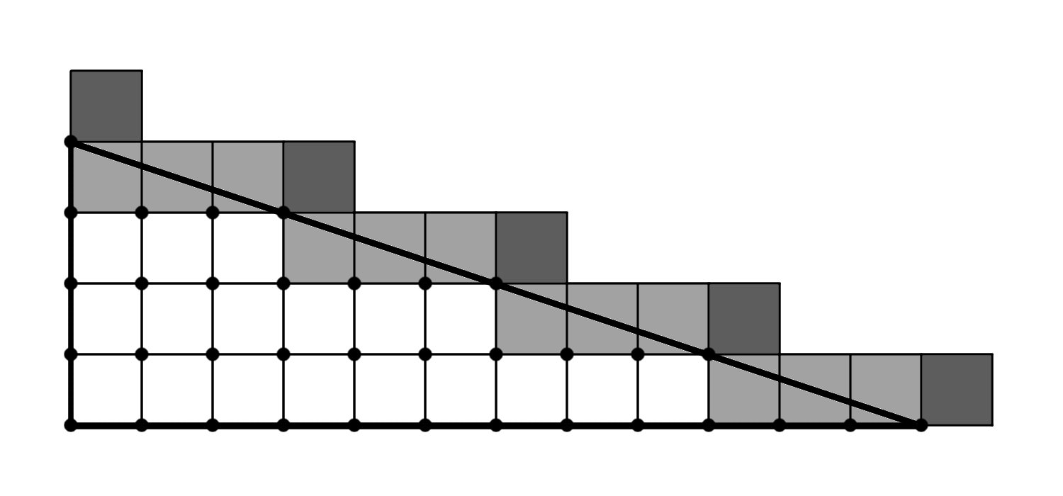
Figure 1: The polytope in this example is a triangle with height 1 and base 3. Furthermore, $k$ = 4. The dots correspond to lattice points in $\mathcal{P}_{3}$. The white squares correspond to the set $P_{{\cal I},3}$, the light gray squares correspond to the set $P_{{\cal F},3}$ and the dark gray squares correspond to the set $P_{\mathcal{E},3}$.

Lemma 8.2.

Let $h$ be a $C^{2}$ function on $B=\Box_{k}(0,\ldots,0)$ and $p_{k,m}$ the midpoint of $B$. Then

$$\left|k^{n}\left(\int_{B}hd\mu\right)-h(p_{k,m})\right|\leq\frac{1}{k^{2}}C_{n}||h||_{C^{2}(B)},$$

where $C_{n}$ only depends on the dimension $n$.

Proof.

First consider the one-dimensional case where $B=[0,\frac{1}{k}]$. Integrating by parts, we see

$$\int_{0}^{\frac{1}{k}}h(x)dx =\int_{0}^{\frac{1}{2k}}h(x)dx+\int_{\frac{1}{2k}}^{\frac{1}{k}}h(x)dx$$

$$=\int_{0}^{\frac{1}{2k}}\left(\frac{x^{2}}{2}+Ax+B\right)h^{\prime\prime}(x)dx-\left.\left.\left(\frac{x^{2}}{2}+Ax+B\right)h^{\prime}(x)\right|^{\frac{1}{2k}}_{0}+(x+A)h(x)\right|^{\frac{1}{2k}}_{0}$$

$$+\int_{\frac{1}{2k}}^{\frac{1}{k}}\left(\frac{x^{2}}{2}+Cx+D\right)h^{\prime\prime}(x)dx-\left.\left.\left(\frac{x^{2}}{2}+Cx+D\right)h^{\prime}(x)\right|_{\frac{1}{2k}}^{\frac{1}{k}}+(x+C)h(x)\right|_{\frac{1}{2k}}^{\frac{1}{k}},$$

where $A,B,C,$ and $D$ are constants that we can choose freely. By choosing $A=B=0$, $C=-\frac{1}{k}$, and $D=\frac{1}{2k^{2}}$, we see that

$$\int_{0}^{\frac{1}{k}}h(x)dx=\frac{1}{k}h\left(\frac{1}{2k}\right)+\int_{0}^{\frac{1}{2k}}\frac{x^{2}}{2}h^{\prime\prime}(x)dx+\int_{\frac{1}{2k}}^{\frac{1}{k}}\frac{\left(x-\frac{1}{k}\right)^{2}}{2}h^{\prime\prime}(x)dx.$$

Hence we have

$$\left|k\int_{0}^{\frac{1}{k}}h(x)dx-h\left(\frac{1}{2k}\right)\right|\leq\frac{1}{24k^{2}}\max_{x\in\left[0,\frac{1}{k}\ \right]}|h^{\prime\prime}(x)|.$$

The proof is completed by induction. Assume the lemma is true for the $n$-dimensional case. Let $h$ be a function of $n+1$ variables. Define $\tilde{h}(x)=h(x_{1},\ldots,x_{n},x)$ and apply the previous argument and the induction hypothesis to get the desired result. ∎

Lemma 8.3.

Let $h$ be a $C^{2}$ function on $P$ and $p_{k,m}$ the midpoint of box $\Box_{k}(p)$. Then we have

$$\left|k^{n}\int_{P_{{\cal I},k}}h(x)dx-\sum_{p\in{\cal I}_{k}}h(p_{k,m})\right|\leq k^{n-2}C_{n}K_{P}||h||_{C^{2}(P)|},$$

where $C_{n}$ is the same constant as the last lemma, and $K_{P}$ is a constant depending on the geometry of $P$.

Proof.

Sum up the previous lemma over the points in ${\cal I}_{k}$. ∎

These lemmas yield a sort of asymptotic estimate for

$$k^{n}\int_{P_{{\cal I},k}}h(x)dx,$$

but in order to estimate the right side of (1.2), we still need an estimate for

$$k^{n}\int_{P\ \backslash\ P_{{\cal I},k}}h(x)dx.$$ (8.3)

We will compare (8.3) to the sum

$$\sum_{p\in{\cal F}_{k}}h(x_{p,k}),$$ (8.4)

where $x_{p,k}$ is some arbitrary point in $B=\Box_{k}(p)$. Note that if $x_{p,k},x_{p,k}^{\prime}\in\Box_{k}(p)$, then

$$|h(x_{p,k})-h(x_{p,k}^{\prime})|\leq\frac{\sqrt{n}}{k}||h||_{C^{1}(B)}.$$ (8.5)

Now let $m_{k}(p)\in\Box_{k}(p)$ be such that $\min_{\Box_{k}(p)}h=h(m_{k}(p))$ and define $M_{k}(p)$ similarly to be where $h$ takes its maximum. We have then that

$$\sum_{p\in{\cal F}_{k}}h(m_{k}(p))\leq k^{n}\int_{P_{{\cal F},k}}h(x)dx\leq\sum_{p\in{\cal F}_{k}}h(M_{k}(p)).$$ (8.6)

Lemma 8.4.

There exists a constant $C$ depending only on the dimension $n$, the geometry of $P$, and $||h||_{C^{1}(P)}$ such that

$$\left|k^{n}\int_{P\ \backslash\ P_{{\cal I},k}}hd\mu-\frac{1}{2}\sum_{p\in{\cal F}_{k}}h(x_{p,k})\right|\leq Ck^{n-2}.$$

where, as before, $x_{p,k}$ is any point in $\Box_{k}(k)$.

Proof.

Given (8.6) and (8.5), we need only show

$$\left|k^{n}\int_{P\ \backslash\ P_{{\cal I},k}}hd\mu-\frac{1}{2}k^{n}\int_{P_{{\cal F},k}}hd\mu\right|\leq Ck^{n-2}.$$ (8.7)

The idea of this proof is the following observation: Assume we are given a rational plane $H\subset\mathbb{R}^{n}$ through the origin which cuts $\mathbb{R}^{n}$ into two pieces $S_{1}$ and $S_{2}$. Furthermore, assume we are given a hypercube $B=\Box_{1}(p)$ such that $H$ intersects the interior of $B$. If $B^{\prime}$ is the hypercube given by reflecting $B$ about the origin, then the pair $(B,B^{\prime})$ has the property that $\mathrm{Vol}(B\cap S_{1})+\mathrm{Vol}(B^{\prime}\cap S_{1})=1$. We will use this idea to prove (8.7) by considering each of the different lattice points in ${\cal F}_{k}$ as our “origin”.

We would ideally like to proceed as follows. Let $p\in{\cal F}_{k}$ be a lattice point and let $q\in\mathcal{E}_{k}$ be the unique point in $\mathcal{E}_{k}$ which is closest to $B=\Box_{k}(p)$. Then let $p^{\prime}$ be the corner point of the box $B^{\prime}$ given by reflecting $B$ about the point $q$.

There are two problems with this approach. The first is that the corresponding point $p^{\prime}$ may not lie in ${\cal F}_{k}$. This will be true for the boxes $B$ which are close to the boundary of $F$. We deal with this problem by not considering the points $p$ which have no corresponding point. The second problem is that the point $q$ need not actually be unique. This could be handled multiple ways, but the easiest seems to be to do the following: Let $d$ be the distance from $B$ to the lattice $\mathcal{E}_{k}$. Let $Q_{B}$ be the set of $q\in\mathcal{E}_{k}$ such that $\mathrm{dist}(B,q)=d$. Let $N_{B}$ the number of elements in $Q_{B}$. Finally consider $N_{B}$ pairs $(B,B^{\prime})$—one for each different $q\in Q_{B}$—and in the end weight each pair by the fraction $\frac{1}{N_{B}}$. This allows us to compare the two integrals in (8.7) with the desired precision. ∎

Taken together, these lemmas result in the following:

Lemma 8.5.

There is a constant $C$ depending only on the geometry of $P$, $||h||_{C^{2}}$, and the dimension $n$ so that

$$\left|k^{n}\int_{P}h(x)-\left(\sum_{p\in{\cal I}_{k}}h(p_{k,m})+\frac{1}{2}\sum_{p\in{\cal F}_{k}}h(x_{p,k})\right)\right|\leq Ck^{n-2},$$ (8.8)

where $x_{p,k}$ is an arbitrary point in $\Box_{k}(p)$ as before.

We are finally in the position to prove Lemma 1.1.

Proof.

To prove this we may assume that $P$ is a “stretched standard simplex”. I.e. that there is a vertex $v$ of $P$, such that if one chooses $v$ as the origin, then $P$ is given as the convex hull of the origin $v$ and the points $p_{1}e_{1},\ldots,p_{n}e_{n}$, where $p_{i}>0$ and $e_{i}$ is the standard basis vector. Any polytope $P$ can be deconstructed into such stretched standard simplices and then if one applies Lemma 1.1 to each piece, one gets the result for all of $P$.

The asymptotic sum $S_{k}$ we need to approximate is given by

$$S_{k}=\sum_{p\in\mathcal{P}_{k}}h(p)=\sum_{p\in{\cal I}_{k}}h(p)+\sum_{p\in{\cal F}_{k}}h(p)+\sum_{p\in\mathcal{E}_{k}}h(p).$$ (8.9)

The main idea of the proof is to compare (8.9) with the “midpoint rule” for integrals. Given (8.8), we only need to understand the asymptotics of the difference $S_{k}-M_{k}$, where

$$M_{k}=\left(\sum_{p\in{\cal I}_{k}}h(p_{k,m})+\frac{1}{2}\sum_{p\in{\cal F}_{k}}h(p_{k,m})\right).$$ (8.10)

Now let $p$ be any lattice point in ${\partial P}\ \backslash\ F$. Let $l_{p,k}(j)=p+\frac{1}{2k}(j,\ldots,j).$ I.e. $l_{p,k}(0)=p$, $l_{p,k}(1)=p_{k,m}$, etc. Let $L_{p,k}=l_{p,k}(\mathbb{R})$ be the line through $p$ parallel to the vector $(1,\ldots,1)$.

Now for each $p$, we will define an alternating sum $A_{p,k}$ as follows. If $p\in{\partial P}\ \cap F$, then define $A_{p}=h(p)$. Otherwise, if $L_{p,k}\cap P$ is a line segment connecting $p$ to an element of $\mathcal{E}_{k}$, define $A_{p,k}$ as

$$A_{p,k}=h(l_{p,k}(0))-h(l_{p,k}(1))+h(l_{p,k}(2))-h(l_{p,k}(3))\pm\cdots+h(l_{p,k}(N)),$$

where we have $l_{p,k}(N)\in\mathcal{E}_{k}$ is that final terminating point. Finally, if $p$ satisfies neither of the preceeding requirements, define

$$A_{p,k}=h(l_{p,k}(0))-h(l_{p,k}(1))+h(l_{p,k}(2))-h(l_{p,k}(3))\pm\cdots+h(l_{p,k}(N-1))-\frac{1}{2}h(l_{p,k}(N)),$$

where $l_{p,k}(N)$ is the midpoint of the box $\Box_{k}(q)$ and $q$ is the point in ${\cal F}_{k}$ which lies on the line $L_{p,k}$.

With this setup, we have that

$$S_{k}-M_{k}=\sum_{p\in{\partial P}\ \backslash\ F}A_{p,k}.$$

Now if $L_{p,k}\cap P$ is a line terminating in a point in $\mathcal{E}_{k}$, then we have that

$$A_{p,k} =\frac{1}{2}h(l_{p,k}(0))+\frac{1}{2}\Bigg{\{}[h(l_{p,k}(0))-h(l_{p,k}(1))]-[h(l_{p,k}(1))-h(l_{p,k}(2))]$$

$$\ \ \ \ +\cdots-[h(l_{p,k}(N-1))-h(l_{p,k}(N))]\Bigg{\}}+\frac{1}{2}h(l_{p,k}(N)).$$

Due to convexity, the middle terms form an alternating series, and hence $A_{p,k}=\frac{1}{2}[h(l_{p,k}(0))+h(l_{p,k}(N))]+\frac{C}{k},$ for some constant $C$ depending on the derivative of $h$. Going back to the case where $L_{p,k}\cap P$ does not terminate in a point in $\mathcal{E}_{k}$, similar arguments show that $A_{p,k}=\frac{1}{2}h(l_{p,k}(0))+\frac{C}{k}$, with $C$ once again depending upon $||h||_{C^{1}(P)}$.

Combining these results we have that up to highest order $S_{k}-M_{k}=\frac{1}{2}\sum_{p\in{\partial P}}h(p)$. If we apply Lemma 8.1, the proof of Lemma 1.1 is complete. ∎

Remark: In the preceeding proof we essentially only used the fact that $h$ is convex along lines parallel to the vector $(1,\cdots,1)$. One may be tempted to conclude that that is all that is necessary for Lemma 1.1. However, in the previous proof we assumed that $P$ was in the form of a stretched standard simplex. If $P$ is arbitrary, we would need to decompose it into stretched standard simplices and apply this result to each one individually. On those other simplices, we would most likely have to change orientations and consider lines that are going in other directions. Hence in general we do need $h$ to be convex in all directions for Lemma 1.1 to be true.

Department of Mathematics
Columbia University, New York, NY 10027
tomnyberg@math.columbia.edu

References

- [1] Abreu, M. Kähler geometry of toric varieites and extremal metrics, International J. Math. 9 (1998) 641-651, MR 99j:58047, Zbl 0932.53043
- [2] Donaldson, S. K. Scalar curvature and stability of toric varieties, Jour. Differential Geometry 62 289-349 2002
- [3] Donaldson, S. K. Interior estimates for solutions of Abreu’s equation, Colectanea Math. 56 103-142 2005
- [4] Donaldson, S. K. Extremal metrics on toric surfaces: a continuity method, Jour. Differential Geometry 79 389-432 2008
- [5] Donaldson, S. K. Constant scalar curvature metrics on toric surfaces, Geometric And Functional Analysis 19 83-136 2008
- [6] Donaldson, S. K. Kähler Geometry on Toric Manifolds, and some other Manifolds with Large Symmetry, Handbook of Geometric Analysis, No. 1. International Press of Boston 2008
- [7] Guillemin, V. Kähler Structures On Toric Varieties, Jour. Differential Geometry 40 285-309 1994
- [8] Humphreys, J. E. Introduction to Lie Algebras and Representation Theory, Graduate Texts in Mathematics, Springer (1973)
- [9] Phong, D. H. and Sturm, J. Lectures on stability and constant scalar curvature”, Current Developments in Mathematics (2009) 101-176, International Press, arXiv: 0801.4179
- [10] Podestà, F. and Spiro, A. Kähler -Ricci solititons on homogeneous toric bundles, J. reine angew. Math. 642 (2010), 109-127
- [11] Raza, A. Scalar curvature and multiplicity-free actions, Ph. D. Thesis, Imperial College London (2005)
- [12] Sepanski, M. R. Compact Lie Groups, Graduate Texts in Mathematics Springer (2006), 151-186