Characterizing the Cool KOIs IV: Kepler-32 as a prototype for the formation of compact planetary systems throughout the Galaxy

Abstract

The Kepler space telescope has opened new vistas in exoplanet discovery space by revealing populations of Earth-sized planets that provide a new context for understanding planet formation. Approximately 70% of all stars in the Galaxy belong to the diminutive M dwarf class, several thousand of which lie within Kepler’s field of view, and a large number of these targets show planet transit signals. The Kepler M dwarf sample has a characteristic mass of 0.5 $M_{\odot}$ representing a stellar population twice as common as Sun-like stars. Kepler-32 is a typical star in this sample that presents us with a rare opportunity: five planets transit this star giving us an expansive view of its architecture. All five planets of this compact system orbit their host star within a distance one third the size of Mercury’s orbit with the innermost planet positioned a mere 4.3 stellar radii from the stellar photosphere. New observations limit possible false positive scenarios allowing us to validate the entire Kepler-32 system making it the richest known system of transiting planets around an M dwarf. Based on considerations of the stellar dust sublimation radius, a minimum mass protoplanetary nebula, and the near period commensurability of three adjacent planets, we propose that the Kepler-32 planets formed at larger orbital radii and migrated inward to their present locations. The volatile content inferred for the Kepler-32 planets and order of magnitude estimates for the disk migration rates suggest these planets may have formed beyond the snow line and migrated in the presence of a gaseous disk. If true, this would place an upper limit on their formation time of $\sim 10$ Myr. The Kepler-32 planets are representative of the full ensemble of planet candidates orbiting the Kepler M dwarfs for which we calculate an occurrence rate of $1.0\pm 0.1$ planet per star. The formation of the Kepler-32 planets therefore offers a plausible blueprint for the formation of one of the largest known populations of planets in our Galaxy.

1. Background

Before the discovery of exoplanets around main sequence stars two decades ago, models of planet formation were based on a solitary example: our own Solar System. Despite the discovery of hundreds, if not thousands of additional planets in the years since then, observational and theoretical efforts have focused on the formation of planets around Sun-like stars. However, the Sun is not a typical star. Seventy percent of stars in the Galaxy are dwarfs of the M spectral class (“M dwarfs” or “red dwarfs,” Bochanski et al. 2010), with masses that are only $\sim 10-50$% the mass of the Sun, much cooler temperatures, and different evolutionary histories. These differences likely result in different formation and evolutionary histories for their planets. For example, both Doppler and transit surveys have revealed a paucity of gas giant planets around M dwarfs, and a relative overabundance of planets with masses less than that of Neptune (Howard et al. 2012). This is in contrast to the high gas giant occurrence rate around stars more massive than the Sun (Johnson et al. 2010a). These correlations between stellar mass and gas giant occurrence are likely a consequence of the lower disk masses around M dwarfs, which result in less raw material available for planet building (Laughlin et al. 2004; Kennedy & Kenyon 2008).

Roughly 5500 of the 160,000 stars targeted by NASA’s Kepler mission are M dwarfs with a mass distribution skewed toward the high mass end of the spectral class (see § 5.1 for details). Of these stars, 66 show at least one periodic planetary transit signal. Aside from a single outlier—the hot Jupiter system around KOI-254 (Johnson et al. 2012)—the ensemble of 100 planet candidates around these M dwarfs have radii ranging from $\sim 0.5$ to 3 $R_{\oplus}$ and semimajor axes within about a few tenths of an astronomical unit (Muirhead et al. 2012a). These compact planetary configurations around the lowest mass stars (e.g., Muirhead et al. 2012b) offer a number of advantages: the signal-to-noise ratio of the transit signals of close-in planets is boosted due to the increased number of transits per observing period (Gould et al. 2003); transit depths are larger for a given planet radius allowing detections of ever smaller planets (Nutzman & Charbonneau 2008); and the reduced temperatures and luminosities of their host stars lead to equilibrium temperatures comparable to the Earth’s, despite their extreme proximity to their stars (Kasting et al. 1993; Tarter et al. 2007).

The Kepler M dwarf planets have been calculated to have an occurrence rate a factor of $\sim 3$ higher than for solar-type stars with occurrence rates increasing as planet size and stellar mass decrease (Mann et al. 2012; Howard et al. 2012). Microlensing studies also suggest a high planet occurrence around low mass stars (Cassan et al. 2012). However, the large errors on these results and the fact that microlensing surveys probe planets at larger separations from their host stars than transit surveys complicate the comparison between samples. The high frequency of small planets around low-mass stars is compounded by the fact that lower mass stars are more common than solar-type stars (Chabrier 2003). Therefore the mechanisms by which small planets form around the lowest mass stars determine the characteristics of the majority of planets currently known to exist in our Galaxy.

Kepler-32 is an M1V star with half the mass and radius of the Sun, roughly two-thirds the Sun’s temperature, and 5% of its luminosity (Muirhead et al. 2012a). While showing 5 distinct transit signals, to date only two of the planets have been validated, Kepler-32 b and c, from the timing variations of their transit signals (TTVs; Fabrycky et al. 2012a). The Kepler-32 host star and its planets are typical of the full Kepler M dwarf sample except for the chance alignment of this system with respect to our line of sight that offers a unique and expansive view of its dynamical architecture. To capitalize on this chance alignment we bring to bear a suite of ground-based observations using the W. M. Keck Observatory and the Robo-AO system on the Palomar 60-inch telescope (Baranec et al. 2012) to validate and characterize the system in detail. We follow this with an in-depth analysis that allows us to place tight constraints on the formation and evolution of the Kepler-32 planets, which in turn has implications for the formation of planets around early M dwarfs in general.

Since all planet parameters are derived directly from the physical characteristics of the host star, we start by refining the stellar properties in § 2. High spatial resolution images and optical spectra are then used by our false positive statistical analyses to validate the remaining three transit signals from the Kepler data in § 3. These above analyses provide the foundation for an accurate characterization of the Kepler-32 planets followed by an investigation into the formation and evolutionary history of this system implied by its observed architecture in § 4. We then turn to a discussion of the ensemble of Kepler M dwarf planets in § 5 and argue that the formation pathway deduced for Kepler-32 offers a plausible blueprint for the formation of planets around the smallest stars, and thus the majority of all stars throughout the Galaxy.

Table 1Observed Stellar Properties

Parameter	Value	Ref.
$\alpha$ (J2000)	19:51:22.18	1
$\delta$ (J2000)	$46^{\circ}34^{\prime}27^{\prime\prime}$	1
$\mu_{\alpha}$ (mas/yr)	-8	1
$\mu_{\delta}$ (mas/yr)	20	1
$K_{P}$	15.801	1
$A_{V}$	0.154	1
$g$	$17.251$	1
$r$	$15.913$	1
$V$	$16.452$	2
$J$	$13.616\pm 0.023$	3
$H$	$12.901\pm 0.024$	3
$K_{s}$	$12.757\pm 0.024$	3
$v_{rad}$ (km s-1)	$-32.5\pm 0.5$	4

References. — (1) Borucki et al. (2011b); (2) Jester et al. (2005); (3) Brown et al. (2011); (4) this work.

2. Kepler-32 Stellar Properties

The observed stellar properties for Kepler-32 are summarized in Table 1. It was originally listed in the Kepler Input Catalog (KIC) with an effective temperature of 3911K, below the 4500 K threshold where the photometric method for determining stellar parameters is deemed reliable (Brown et al. 2011). Follow-up, medium-resolution infrared spectroscopy presented by Muirhead et al. (2012a) revised and refined the KIC values to $T_{\rm eff}=3727^{+102}_{-58}$ and [Fe/H]$=0.04\pm 0.13$.

In this work we supplement these measurements with an independent estimation of the stellar mass, radius and metallicity using the broadband photometric method presented by Johnson et al. (2012). This method evaluates the posterior probability distribution of each stellar parameter conditioned on the observed apparent magnitudes and colors of the star listed in the KIC using model relationships such as the Delfosse et al. (2000) mass-luminosity relation and the West et al. (2005) color-spectral-type relation. Our Markov Chain Monte Carlo analysis yields $M_{\star}=0.57\pm 0.06$ $M_{\odot}$, $R_{\star}=0.53\pm 0.04$ $R_{\odot}$, and [Fe/H]$=-0.05\pm 0.17$.

We combine the results of the above analyses with those of Borucki et al. (2011a), Muirhead et al. (2012a), and Fabrycky et al. (2012a) by weighted mean to obtain the final values used in this work presented in Table 2.1. We adopt 10% errors on the Borucki et al. (2011a) values for stellar mass and radius. For the effective temperature, we construct probability distribution functions and compute the mean and $1\,\sigma$ errors numerically to account for the asymmetric errors in the Muirhead et al. (2012a) value. Using the Delfosse et al. (2000) $K$-band mass-luminosity relationship we find that our final stellar mass and its uncertainty give a distance modulus of $7.407\pm 0.098$, corresponding to a distance of $d=303\pm 14$ pc.

2.1. Stellar Age

It is difficult to measure the age of field M dwarfs unassociated with known moving groups or clusters because their global stellar properties change little over the course of their main sequence lifetime. However, Kepler-32 has a slow rotation rate of $P=37.8\pm 1.2$ days measured from the modulation of the light curve by star spots (Fabrycky et al. 2012a) implying that it is old. To estimate the age of Kepler-32 we use the age equation from Barnes (2010),

$$t=\frac{\tau}{k_{C}}\ln\left(\frac{P}{P_{0}}\right)+\frac{k_{I}}{2\tau}\left(P^{2}-P_{0}^{2}\right).$$ (1)

The dimensionless constants $k_{C}=0.646$ days Myr^-1 and $k_{I}=452$ Myr day^-1 are determined observationally, the convection turnover time is estimated as $\tau=k_{I}/2\cdot f^{2}(B-V)$, where we use $f(B-V)=0.77(B-V-0.4)^{0.6}$ (Barnes 2007) and $(B-V)=1.5$ (converted from $g-r$ using Jester et al. 2005) to give $\tau=155$ days. Using the median value of the initial spin period, $P_{0}=2.81$, as required to produce the observed rotation rates for $\approx 0.6$ $M_{\odot}$ stars in the Praesepe cluster (Agüeros et al. 2011) we derive an age of 2.7 Gyr for Kepler-32. The large scatter in observed rotation rates for Praesepe members used here to calibrate $P_{0}$ suggests the age of Kepler-32 could be as young as 2.3 Gyr or as old as 3.7 Gyr. For this work we will assume that the age of Kepler-32 is greater than $2$ Gyr.

Table 2Derived Stellar Properties

Parameter	KIC	M12	F12	this work	Adopted Values
$T_{\rm eff}$ (K)	$3911\pm 200$	$3727^{+102}_{-58}$	$3900\pm 200$	$\cdots$	$3793^{+80}_{-74}$
$M_{\star}$ ($M_{\odot}$)	$0.49\pm 0.05$	$0.52\pm 0.04$	$0.58\pm 0.05$	$0.57\pm 0.06$	$0.54\pm 0.02$
$R_{\star}$ ($M_{\odot}$)	$0.56\pm 0.06$	$0.50\pm 0.04$	$0.53\pm 0.04$	$0.53\pm 0.04$	$0.53\pm 0.02$
$[$Fe/H$]$	$-0.056\pm 0.2$	$0.04\pm 0.13$	$0\pm 0.4$	$-0.05\pm 0.17$	$-0.01\pm 0.09$
$d$ (pc)	$\cdots$	$\cdots$	$\cdots$	$303\pm 14$	$303\pm 14$
age (Gyr)	$\cdots$	$\cdots$	$\cdots$	$\sim 2.6$	$>2$

References. — (1) Brown et al. (2011); (2) Muirhead et al. (2012a); (3) Fabrycky et al. (2012a)

3. Validation of Transit Signals

Two of the Kepler-32 planets (b and c) have been validated previous to this study using signatures of their mutual dynamical interactions (Fabrycky et al. 2012a). The other three transit signals have hitherto retained the status of planet candidates. The probabilities for Kepler planet candidates to be astrophysical false positives, such as blended stellar eclipsing binaries, are generally low (Morton & Johnson 2011), and may even be negligible in multiply transiting systems (Lissauer et al. 2012). Diffraction limited images in the Kepler band made with the Robo-AO system on the Palomar 60-inch telescope (Baranec et al. 2012) show no evidence of blended companions for a $5\,\sigma$ contrast of $\Delta z\approx 3.5$ at $0^{\prime\prime}\!\!.5$ and $\Delta z\approx 4.5$ at $1^{\prime\prime}$. High-resolution optical spectroscopy with the HIRES spectrograph on Keck I and high-resolution adaptive optics imaging in the near infrared using the NIRC2 camera on Keck II place stringent constrains on the probabilities of various false positive scenarios, allowing a probabilistic validation of the transit signals using the procedure of Morton (2012).

3.1. Keck I/HIRES Spectroscopy

We obtained spectra of Kepler-32 at Keck Observatory using the HIgh-Resolution Echelle Spectrometer (HIRES, Vogt et al. 1994) on Keck I with the standard observing setup used by the California Planet Survey (Johnson et al. 2010b) which covers a wavelength range from 3640Å to 7820Å. Because of the star’s faint visual magnitude we used the C2 decker corresponding to a projected size of $14^{\prime\prime}\!\!.0\times 0^{\prime\prime}\!\!.851$ to allow sky subtraction and a resolving power of $R=55000$. We obtained 2 observations of Kepler-32 (UT 18 June 2011 and UT 13 March 2012), both with an exposure time of 700 seconds, each resulting in a signal-to-noise ratio (SNR) of 20 at 6500Å.

To measure the systemic radial velocity of Kepler-32 and to check for evidence of a second set of stellar lines in the spectrum, we performed a cross-correlation analysis with respect to a HIRES spectrum of a similar star (HIP 86961: $V_{rad}=-28.9\pm 0.4$ km s^-1; Nidever et al. 2002) using the methodology described by Johnson et al. (2010a). Our analysis yields a systemic radial velocity of $-32.5\pm 0.5$ km s^-1. No second set of lines are evident above the noise floor in the cross-correlation function, allowing us to rule out stellar companions with $V>10$ km s^-1 and $V$-band brightnesses within 2 magnitudes.

3.2. Keck II/NIRC2 Adaptive Optics Imaging

We performed adaptive optics imaging using the NIRC2 instrument on the Keck II telescope on UT 24 June 2011 to rule out false positive scenarios involving blended sources. With a Kepler bandpass magnitude $K_{P}=15.80$, Kepler-32 is relatively faint for natural guide star observations. Nevertheless, we were able to close the adaptive optics (AO) system control loops on the star with a frame rate of 41 Hz. With sufficient counts in each wavefront sensor subaperture, a stable lock was maintained for the duration of the observations.

Figure 1.— $J$ and $K^{\prime}$ band contrast curves derived from our Keck II/NIRC2 adaptive optics imaging constrain false positive scenarios involving blended sources.

We acquired two sets of dithered images using the NIRC2 medium camera (plate scale = 20 mas pix^-1) a sequence of 9 images in the $J$-filter (central wavelength = 1.25 $\mu$m), and a sequence of 9 images in the $K^{\prime}$-filter (central wavelength = 2.12 $\mu$m). Each image had an exposure time of 20 s, resulting in a total on-source integration time of 180 s per filter. To process the data, hot pixels were removed, the sky-background was subtracted, and the images were aligned then coadded. We measured the contrast achieved by NIRC2 adaptive optics imaging by comparing the peak intensity of the star in the final processed image to the intensity of residual scattered starlight at small angular separations. Specifically, we calculate the standard deviation of flux, $\sigma$, within a box of size $3\times 3$ FWHM, where FWHM is the point-spread function full-width at half-maximum spatial scale (also the size of a speckle). The standard deviation is evaluated at numerous locations close to the star and the results are azimuthally averaged to estimate the local radial contrast profile. Figure 1 shows the $5\,\sigma$ contrast curves based on each reduced AO image. The full instrument field of view is $20^{\prime\prime}\times 20^{\prime\prime}$, which corresponds to 5 Kepler pixels on a side. No obvious contaminants were identified within $\Delta K^{\prime}=6.5$ at a separation of $0^{\prime\prime}\!\!.7$ or farther from Kepler-32.

3.3. Kepler Light Curves

Our light curve data come from the Kepler space telescope, which is conducting a continuous photometric monitoring campaign of a target field near the constellations Cygnus and Lyra. A 0.95-m aperture Schmidt telescope feeds a mosaic CCD photometer with a $10^{\circ}\times 10^{\circ}$ field of view (Koch et al. 2010; Borucki et al. 2011b). Data reduction and analysis is described by Jenkins et al. (2010a, b) and photometric and astrometric data were made publicly available as part of the 28 July 2012 public data release. We downloaded the data from the Multimission Archive at STScI (MAST), and we use the pipeline-corrected light curves from Quarters 0 through 9 (Batalha et al. 2012).

These light curves were aggressively detrended to take out all astrophysical variation by first masking out all transit signals and then sequentially fitting a low-order polynomial to the time series data in 2 day chunks. These detrended data were then folded for each Kepler-32 d, e and f with the other planet signals masked according to the ephemeris of Fabrycky et al. (2012a). These folded transit signals were used for the FPP analysis. The binned photometric data are shown in Figure 2 with the trapezoidal fits used to assess the transit shape overlaid.

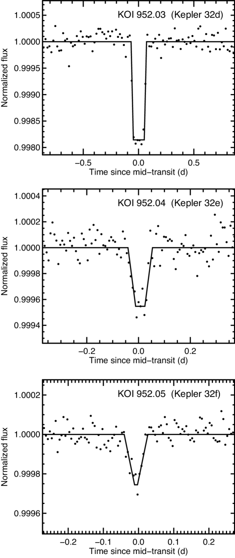
Figure 2.— Detrended, folded and binned Kepler lightcurves for the three planets that we validate with our FPP analysis. The trapezoidal fits from the analysis of Morton (2012) are overlaid.

3.4. False Positive Probability Analysis

To calculate the relative probabilities of astrophysical false positive and bona fide transiting planet scenarios, we follow the methodology of Morton (2012), which compares the observed transit shapes to those of simulated false positive populations, subject to the available observational constraints. Although occurrence rates may be as high as 10% for planets in the radius bins corresponding to KOI-952.03, .04, and .05 (Howard et al. 2012) we assume a very conservative occurrence rate of 1%.

Figure 3 summarizes these FPP results for all three signals. Despite our conservative estimates of planet occurrence rate and without accounting for the fact that Kepler-32 b and c have already been confirmed to be coplanar transiting planets, which would further decrease the FPPs by a factor of about 10, we estimate the FFPs for KOI-952.03, .04, and .05 to all be less than 0.3%. We therefore consider all five photometric signals to be fully validated planet transits making Kepler-32 the richest known system of transiting planets around an M dwarf, and we assign the names Kepler-32 d, e, and f to the former candidates KOI-952.03, .04, and .05, respectively. Verification of the transit signals allows us to take full advantage of the fortuitous alignment of the Kepler-32 system with respect to our line of sight, and in the next section we look deeper into the details and implications of its specific configuration.

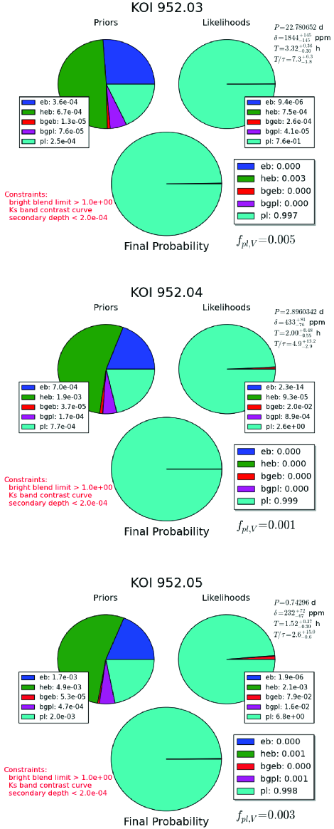
Figure 3.— The relative strength of each possible scenario in our false positive calculation—eclipsing binary (eb), hierarchical binary (heb), background eclipsing binary (bgeb), background planet (bpl) and planet (pl)—is shown pictorially for our priors (upper left chart), likelihood (upper right chart), and final probability (lower chart) for each KOI-952.03 (top panel), .04 (middle panel), and .05 (bottom panel). Observational constraints used in the calculation are stated in red (lower left) and the trapezoidal fit paramters are shown (upper right) in each panel. The quantity $f_{pl,V}$ is the smallest value of the planet occurrence that would result in validation for the given transit signal.

Table 3Derived Planet Properties

KOI	Kepler	$P$	$a$	$R_{p}$	$T_{eq}$
		($days$)	($AU$)	($R_{\oplus}$)	($K$)
952.05	32f	0.74296(7)	0.0130(2)	0.81(5)	1100
952.04	32e	2.8960(3)	0.0323(5)	1.5(1)	680
952.01	32b	5.9012(1)	0.0519(8)	2.2(1)	530
952.02	32c	8.7522(3)	0.067(1)	2.0(2)	470
952.03	32d	22.7802(5)	0.128(2)	2.7(1)	340

References. — (1) Fabrycky et al. (2012a)

4. The Kepler-32 Planetary System

The increased accuracy with which we derive the stellar parameters for Kepler-32 (see Table 2.1) leads to more precise planetary parameters, which we outline in Table 3.4. The planets of Kepler-32 have radii that are similar to values found in the Solar System, from below Earth size up to about 70% of Neptune. However, the planetary system of Kepler-32 has a remarkably distinct dynamical architecture in comparison. Figure 4 shows the relative sizes of the planets and their orbits, along with labels denoting their periods, semimajor axes and period commensurabilities rounded to the nearest integer. The five planets of this system orbit within 0.13 AU from the star, or approximately one third of Mercury’s semimajor axis. The outermost planet lies within a region where the stellar insolation is similar to Earth’s, while at the other extreme, the innermost planet orbits only 4.3 stellar radii from the photosphere of Kepler-32. The three middle planets—termed e, b, and c in order of increasing semimajor axis—exhibit period ratios within 2% of a 1:2:3 commensurability.

4.1. Tidal Evolution

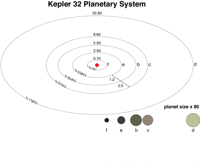
Figure 4.— Depiction of the Kepler-32 planetary system with the star and orbits drawn to scale. The relative sizes of the planets are shown at the bottom of the figure scaled up by a factor of $80$ in relation to their orbits.

The proximity of the Kepler-32 planets to their host star imply that their dynamics have been significantly altered due to tidal forces induced by the host star over the age of the system. Using an initial spin period of 10 hours, a tidal dissipation factor of 100, a rigidity factor of $3\times 10^{11}$ and a density profile similar to Earth such that the moment of inertia $I\approx 0.5\,M_{p}R_{p}^{2}$, we derive the tidal locking timescales for the Kepler-32 planets to all be $\lesssim 1$ Myr (Murray & Dermott 2000). This timescale depends linearly on the dissipation factor, $Q$, which is highly uncertain for exoplanets. However, for a reasonable range of $Q$ values ranging up to $10^{5}$ it can be expected that the rotation periods of all the planets in the Kepler-32 system are equal to their orbital period barring spin-orbit resonances.

Tidal forces from the host star will also damp the eccentricities of the planets in direct proportion to $Q$ (Murray & Dermott 2000). For $Q<10^{4}$ the inner planets will have no free (primordial) eccentricity. Though even for a low $Q$, the tidal damping time for Kepler-32 d, the most distant planet, is approximately 4 Gyr, comparable to the age of the system. The free eccentricities of Kepler-32 b and c have recently been estimated to have non-zero values from the phase of the TTV signals (Lithwick et al. 2012; Wu & Lithwick 2012). This suggests high $Q$ values for these planets, consistent with their moderate inferred densities (see § 4.2).

Contrary to the trend for Kepler pairs to lie longward of mean motion resonance (Fabrycky et al. 2012b), Kepler-32 b and c lie 1.1% shortward of resonance. The high $Q$ values suggested above would limit dissipative mechanisms that may spread their orbits (Lithwick & Wu 2012; Batygin & Morbidelli 2012). Also Kepler-32 b is near a 2:1 resonance with Kepler-32 e. However, our n-body simulation of § 4.4 suggests planet e has too small an effect to account for these effects.

4.2. Mass and Density Estimates

As mentioned above, Kepler-32 b and c were validated based on the TTVs observed due to their mutual interactions (Fabrycky et al. 2012a). The amplitude of the TTV signals specify upper limits to their masses of be 6.6 and 8.4 $M_{\oplus}$, implying densities of less than 3.4 and 5.7 g cm^-3 for b and c respectively (Lithwick et al. 2012). However, the TTV phases are measured to be $\sim 45^{\circ}$ from $0$ and $\pi$ implying a small free eccentricity. A correction for this effect by Wu & Lithwick (2012) reduce the estimated masses for Kepler-32 b and c by factors of $0.51$ and $0.45$. With these corrections the masses and densities for Kepler-32 b and c are 3.4 and 3.8 $M_{\oplus}$ and 1.7 and 2.6 g cm^-3. The nominal masses for Kepler-32 b and c imply mass-radius relationships of $M\propto R^{\gamma_{p}}$, with $\gamma_{p}=1.5-1.9$, similar to the value of 2.06 for the six Solar System planets bounded by Mars and Saturn (Lissauer et al. 2011).

The above stated densities imply that Kepler-32 b and c are composed of a significant amount of volatiles. Using Equations 7 and 8 of Fortney et al. (2007), we find that if Kepler-32 b and c had no atmospheres they would be expected to contain $\sim 96\%$ and $\sim 56\%$ volatiles. However, given the equilibrium temperatures of Kepler-32 b and c a large fraction of their volatile content likely exists in the form of an atmosphere.

4.3. Atmospheric Evolution

The proximity of the Kepler-32 planets to their host star suggest significant atmospheric evolution due to evaporation, outgassing or both processes. The equilibrium temperature of Kepler-32 f is $\sim 1100$ K and its radius is measured to be 0.81 $R_{\oplus}$. For a planet this small with such a high equilibrium temperature the atmospheric mass fraction would have to be very small, $\sim 10^{-5}$ (Rogers et al. 2011). Using an extreme ultraviolet luminosity of Kepler-32, $L_{EUV}\approx 10^{26.6}$ (Hodgkin & Pye 1994) and following Lecavelier Des Etangs (2007) using a conservative mass loss efficiency of $\epsilon_{UV}=0.1$ we derive an atmospheric mass loss of $\sim 10^{8}$ g s^-1. Thus the timescale to lose its atmosphere is more than 100 times shorter than the age of the Kepler-32 system. We therefore conclude the Kepler-32 f contains no atmosphere.

Given the size and equilibrium temperature of Kepler-32 e its atmospheric mass fraction must also be small, $M_{a}/M_{p}\sim 10^{-4}$ while the present day atmospheric mass loss rate is between $10^{7}$ and $10^{8}$ g s^-1. The timescale for the complete loss of the Kepler-32 e atmosphere is calculated to be between 0.2 and 2 Gyr. Therefore Kepler-32 e must have lost a significant fraction of any atmosphere it started with.

The total atmospheric mass loss for the other three planets is at least $\sim 10^{-4}$ $M_{\oplus}$ for reasonable choices of planetary mass. If these planets have relatively low-density cores (ice and rock) and started out with large atmospheres, they could have suffered considerable atmospheric evolution due to the heating by Kepler-32. Thus the observed sizes of the Kepler-32 planets are likely determined in part by the extreme ultraviolet and X-ray luminosity of their host star. However, the mass estimates from § 4.2 suggest that Kepler-32 b is 10% less massive than Kepler-32 c while being 10% larger and 25% closer to Kepler-32 hinting that the mass-radius relation for the Kepler-32 planets is not determined solely by a simple atmospheric evolution model.

4.4. Kepler-32 Planetary System Architecture

The physical characteristics of the Kepler-32 planets are summarized in Table 3.4 and the remarkably compact and orderly architecture of the system is shown schematically in Figure 4. As mentioned above, three of the planets lie within 2% of a 1:2:3 period commensurability. Kepler-32 e and b have a period ratio of 2.038, which is 1.9% longward of commensurability, while Kepler-32 b and c have a period ratio of 1.483, or 1.1% shortward of commensurability.

Planets within a mean motion resonance can stray a few percent from commensurability and maintain the libration of resonant angles (Murray & Dermott 2000). However without detailed knowledge of the individual orbits it is not possible to determine with certainty if a planet pair is in a resonant configuration. Therefore we assess the significance of the near commensurability of Kepler-32 e, b, and c using a probabilistic argument.

We randomly populate 5 planet systems with periods between the inner and outermost planets in the Kepler-32 system enforcing separations larger than $2\sqrt{3}$ for every pair of neighboring planets (Gladman 1993) and larger than 9 for chains of planets (Chambers et al. 1996; Smith et al. 2009; Lissauer et al. 2011) in units of mutual Hill radii. In this section a mass-radius relationship of $M\propto R^{2.06}$ (Lissauer et al. 2011) is adopted for consistency. The final ensemble of systems provide a baseline against which we can gauge the significance of the Kepler-32 architecture. The occurrence of period ratios in our randomly drawn sample that lie within either the observed period ratio of Kepler-32 e and b, or b and c, is fairly high, 11% and 12%, respectively. However the fraction of systems arranged in a chain involving any combination of 1:2 or 2:3 near-commensurabilities is $1.9\%\pm 0.5\%$. This suggests that the architecture we observe today reflects the result of dynamical evolution rather than a result of chance.

Given the compactness of the Kepler-32 system, we expand on the dynamical stability simulations of Fabrycky et al. (2012a) by considering all five planets. Kepler-32 f is very likely on a circular orbit and lies $>30$ mutual Hill radii away from the nearest planet. It therefore is not expected to have any bearing on the stability of the system (Smith & Lissauer 2009) and is not included in the following analysis.

Using the Mercury6 software (Chambers 1999) employing the hybrid symplectic Bulirsch-Stoer integrator we integrate the Kepler-32 system for 30 Myr, or $\sim 500$ million orbits of the outermost planet. Our initial conditions were set according to the ephemeris of Fabrycky et al. (2012a) with an initial time step of one tenth the orbital period of the innermost planet (in this case, Kepler-32 e). We began with zero eccentricity and random inclinations drawn uniformly between the minimum and maximum values that would produce a transit from our vantage point. We did not include any tidal effects. The eccentricities and inclinations varied stably with small amplitudes. Figure 5 shows the inclination evolution resampled at 100 kyr time steps and histograms of the eccentricities measured every 100 yrs over the 30 Myr simulation for the outer four planets.

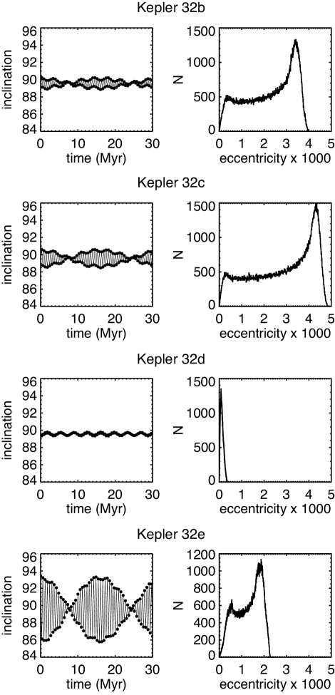
Figure 5.— Time evolution of the inclinations sampled every 100kyr and the distributions of eccentricities for the Kepler-32 planets sampled every 100 yrs from our n-body simulation. Kepler-32 f was not included in the simulation due to its dynamical isolation from the rest of the planetary system (see text).

4.5. The Formation and Evolution of the Kepler-32 Planetary System

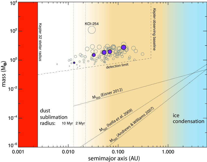
Figure 6.— The masses of the Kepler-32 planets (purple dots) at their respective semimajor axes are shown in relation to the full distribution of M dwarf planet candidate masses (gray circles) calculated according to $M\propto R^{2.06}$ except for Kepler-32 b and c for which we use the masses from § 4.2. The isolation masses of three different disk models are labeled ($M_{iso}$, dotted lines). Also shown are conservative locations of the dust sublimation radius for pre-main sequence ages of 2 Myr and 10 Myr (Baraffe et al. 1998), the approximate location of the ice line during the planet forming epoch (blue shaded region, Kennedy & Kenyon 2008), and the stellar radius of Kepler-32. The discovery space of the Kepler mission through quarter 6 (from which this sample is drawn) is roughly delineated with the thin dashed lines.

The long-term stability evident in our simulation of § 4.4 allows us to view the present-day architecture of the Kepler-32 planets as representing the state of the system at the end of its formation epoch, $\sim 10-100$ Myr after the formation of the star. We now investigate what can be learned about the formation of the Kepler-32 planets by looking backward from their end state.

4.5.1 The Kepler-32 Protoplanetary Nebula

Planets form from flattened disks of dust and gas circulating around protostars, and the masses and sizes of these protoplanetary disks as well as their lifetimes and accretion rates are constrained from observations (see Williams & Cieza 2011). The surface density profiles are typically assumed to follow a power law form $\Sigma_{d}\propto a^{-\gamma}$. (Note: Here and throughout we use $a$ to denote both the orbital radius of circumstellar material and the semimajor axis of the planets. The Kepler planets typically have low eccentricities (Wu & Lithwick 2012) minimizing ambiguity.)

The value of $\gamma$ is often taken to be $3/2$ based on estimates of the “minimum mass solar nebula” (MMSN; Weidenschilling 1977; Hayashi 1981). The MMSN is constructed by smoothing the planets of the Solar System over their respective domains and correcting for Solar abundance to recreate a minimal surface density profile from which the Solar System could have formed. Modern observations constrain the surface density profile in the outer disk ($\gtrsim 40$ AU) to be on average shallower than this, $\gamma\approx 0.4$–1.0 (Andrews & Williams 2007; Isella et al. 2009; Andrews et al. 2009), while the form of the surface density profile in the inner disk remains largely unconstrained.

We can construct a “minimum mass protoplanetary nebula” for Kepler-32 in a similar fashion. Since we do not have mass estimates for all the planets in the Kepler-32 system we use the mass-radius relationship for Solar System planets $M\propto R^{2.06}$ (Lissauer et al. 2011), consistent with the nominal masses from § 4.2 to within 50%. Assuming a gas-to-dust ratio of 100 and a rocky core mass fraction of 50% implies that the protoplanetary nebula of Kepler-32 contained $\approx 3\,M_{Jup}$ of gas between 0.013 and 0.13 AU of the host star.

This translates to a very high surface density, $\approx 5\times 10^{5}$ g cm^-2, in the inner regions of the disk that is incongruous with the masses and surface density profiles in the outer regions of disks as measured with (sub)-millimeter interferometry (Andrews & Williams 2007; Isella et al. 2009; Andrews et al. 2009). Indeed, if this surface density is used to scale the median best fit values of the disk radius and surface density profile index for stars less than 1 $M_{\odot}$ in the Andrews et al. (2009) sample—$R_{d}=126$ AU and $\gamma=0.9$—the total mass of the Kepler-32 protoplanetary nebula would be orders of magnitude greater than the star! This implies one of three possibilities: the disk surface density deviated significantly from a single powerlaw in the inner regions with a large pile-up of material near the disk inner radius (see, e.g., Chiang & Laughlin 2012); the material that formed the planets came from elsewhere in the disk; or the planets themselves formed elsewhere and were transported to their present-day locations.

4.5.2 Oligarchic Growth and the Isolation Mass

The gravitational influence of the host star poses another barrier to super-Earth-sized planets forming within a tenth of an AU. The amount of material accessible to a growing planetary embryo during the oligarchic phase of growth is estimated by the “isolation mass” (Lissauer 1987). This quantity is derived by calculating the amount of mass available to an oligarch within a disk of planetesimals. We choose the radius of gravitational influence to be $4$ Hill radii based on the approximate spacing of isolated oligarchs in numerical simulations (Kokubo & Ida 1998) to obtain

$$M_{iso}=\frac{\left[16\pi a^{2}\Sigma(a)\right]^{3/2}}{(3M_{\star})^{1/2}}$$ (2)

where $a$ is the radial distance from the star, $M_{\star}$ is the mass of the star, and $\Sigma(a)$ is disk surface density profile. To calculate values for $M_{iso}(a)$, we again use the median surface density profile of the M stars in the Andrews et al. (2009) sample, the median values of the M stars in the Isella et al. (2009) sample with $\gamma=0.5$ and $R_{d}=260$ AU, and also the Eisner (2012) model with a median disk radius of $R_{d}=250$ AU and a surface density profile with fixed $\gamma=1.37$ based on theoretical arguments.

Figure 6 shows that the isolation mass computed for these surface density models are $\gtrsim 3$ orders of magnitude too small to account for the mass in the Kepler-32 planets. While the planetary embryos can undergo an additional phase of growth through subsequent mergers that increase their mass by an order of magnitude (e.g., Chambers & Wetherill 1998), it would be difficult to achieve an additional factor of $\sim 100$ growth during this phase (see also Lissauer 2007). The total amount of growth in this late phase growth is limited to the total amount of mass present in the disk at the outset, which is addressed in the previous section.

The migration of planetesimals from outside this region also offers a possibility for late time growth of the Kepler-32 planets (Hansen & Murray 2012). However the gravitational stirring of the planetesimals can cause radial displacements of the planetary embryos away from period commensurability. The magnitude of this effect has recently been used to place limits on the amount of mass contained in orbit-crossing planetesimals at the end stages of planet formation for closely spaced, low inclination multi-planet Kepler systems (Moore et al. 2012). These limits of $\sim 1$ $M_{\oplus}$ are too low to contribute significantly to the discrepancy between the isolation mass and the final mass of the Kepler-32 planets.

This corroborates the above conclusions that the Kepler-32 protoplanetary disk either contained a disproportionately large amount of mass within 0.1 AU, or that the formation of the Kepler-32 planets followed a more complex formation and evolution history.

4.5.3 The Dust Sublimation Radius

Planets form from dust in protoplanetary disks. But at small orbital radii the stellar irradiation raises the dust temperature beyond the sublimation point, clearing these regions of the raw materials for planet formation. Low-mass stars such as Kepler-32 begin pre-main sequence evolution with luminosities much larger than their main sequence values and take $>10$ Myr to contract to the point when hydrogen burning begins. The sublimation radius at these early epochs is thus further from the star than one would conclude from the present-day luminosity of the star.

The dust sublimation radius is given as

$$R_{sub}=0.034\left(\frac{1500}{T_{sub}}\right)^{2}\sqrt{\frac{L_{\star}}{L_{\odot}}\left(2+\frac{1}{\epsilon}\right)}$$ (3)

(Isella et al. 2009) where $T_{sub}$ is the sublimation temperature of the dust, $L_{\star}$ is the stellar luminosity, and $\epsilon$ is a measure of the cooling efficiency of the grains with larger grains having higher efficiencies leading to smaller sublimation radii (Isella et al. 2006). Figure 7 shows the evolution of $R_{sub}$ as a function of pre-main sequence age of a 0.5 $M_{\odot}$ star based on the stellar evolution models of Baraffe et al. (1998).

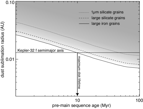
Figure 7.— Dust sublimation radius of Kepler-32 as a function of pre-main sequence age according to the models of Baraffe et al. (1998). The solid curve is for large iron grains ($T_{sub}=1908$ K and $\epsilon=1$) the dashed curve is for large silicate (olivine) grains ($T_{sub}=1774$ K and $\epsilon=1$), and the dotted curve is for 1 $\mu$m silicate (olivine) grains within a lower density environment ($T_{sub}=1570$ K and $\epsilon=0.58$). All curves cross the present day semimajor axis of Kepler-32 f after the typical lifetime of a protoplanetary disk.

Even if it is conservatively assumed that the dust is in large grains ($\epsilon=1$) and composed of pure iron with a sublimation temperature $T_{sub}=1908$ K (Pollack et al. 1994), the sublimation radius does not move inward of Kepler-32 f’s orbit until after 9.8 Myr of pre-main sequence evolution. For smaller grains made of silicates and for less dense environments the dust sublimation radius lies beyond the semimajor axis of Kepler-32 f until after $\sim 50$ Myr, and beyond the present day orbit of Kepler-32 e for $\sim 3$ Myr of pre-main sequence evolution. This poses a serious challenge to in situ formation particularly since the dusty disks from which planets form only last $\lesssim 10$ Myr before they are drained, disrupted, or evaporated away (Williams & Cieza 2011).

4.5.4 In Situ Formation vs. Formation then Migration

The above investigation into the structure of the Kepler-32 planetary system as well as the history and evolution of the host star present meaningful constraints on its formation. To form Kepler-32 f and e where we view them today requires that they formed from planetesimals scattered inward from the wider orbit planets. This kind of formation scenario would be different than the theory described by Hansen & Murray (2012) where scattered planetesimals accrete onto pre-existing oligarchs from an early phase of planet formation. Rather Kepler-32 f and e would have had to have formed from scattered planetesimals in a region largely devoid of solid material. It is not clear how feasible this would be, and requires an investigation beyond the scope of this work. An additional challenge for in situ formation of the Kepler-32 planets is to explain the near period commensurabilities of Kepler-32 e, b and c with in situ formation that we have shown to be statistically significant beyond pure chance.

On the other hand, a scenario in which the Kepler-32 planets formed further out in the disk and then migrated to their present locations offers a natural explanation for 1) the large amount of planetary mass within 0.1 AU of this 0.54 $M_{\odot}$ star, 2) the position of Kepler-32 f within the dust sublimation radius of the star for $\sim 10$ Myr of pre-main sequence evolution, and 3) the near period commensurabilities between three of the planets. The high volatile content inferred for Kepler-32 b and c is also indirect evidence that these planets may have acquired volatiles from beyond the snow line at $\sim 1$ AU (Kennedy & Kenyon 2008). The difficulties in applying this concept lie in understanding the mechanisms of migration through a disk of gas and planetesimals. While a full, rigorous analysis of these possibilities is also beyond the scope of this article, we look to some order of magnitude calculations of different migration mechanisms for insight.

4.5.5 Migration

The compact and coplanar architecture of the Kepler-32 system favors migration through a disk rather than through planet-planet interactions. Interactions with either a gaseous disk or a disk of planetesimals can cause radial migration of planetary orbits (see Kley & Nelson 2012, for a review). Planets massive enough to open a gap in the protoplanetary disk are coupled to the viscous evolution of the disk while less massive planets migrate more quickly due to larger disk torques.

Using a generalized criterion for gap formation in a viscous disk (Crida et al. 2006, Eq. 15) we find that none of the Kepler-32 planets would have opened a gap in their protoplanetary disk assuming a constant disk flaring term $a/H=0.05$ where $H$ is the scale height, a viscosity parameter $\alpha=10^{-3}$ and using the nominal masses for Kepler-32 b and c (§ 4.2) and $M_{p}\propto R_{p}^{2.06}$ otherwise. We therefore restrict our discussion of migration through a gaseous disk to the “type I” mechanism (Goldreich & Tremaine 1979; Lin & Papaloizou 1979)

Assuming a protoplanetary disk with with a powerlaw surface density profile, $\Sigma=\Sigma_{0}a^{-\gamma}$, and a midplane temperature profile, $T\propto a^{-\beta_{T}}$, we estimate the migration rate through a gaseous disk following Kley & Nelson (2012)

$$\frac{da}{dt}=\Gamma_{\rm tot}\frac{2}{m_{p}}\sqrt{\frac{a_{p}}{GM_{\star}}}$$ (4)

where $p$ subscripts refer to planet quantities, and $\Gamma_{\rm tot}$ is the total torque on the planet from Linblad, corotation, and horseshoe torques

$$\Gamma_{\rm tot}=\left[-1.36+0.62\gamma+0.43\beta_{T}+1.36(3/2-\gamma)\right]\Gamma_{0}$$ (5)

(also see Masset et al. 2006), and

$$\Gamma_{0}=\left(\frac{m_{p}}{M_{\star}}\right)^{2}\left(\frac{H}{a_{p}}\right)^{-2}\Sigma_{p}a_{p}^{4}\Omega_{p}^{2}.$$ (6)

As a baseline model we use a disk surface density profile with $\gamma=1$, which extends from the present day location of Kepler-32 f out to 200 AU, contains a total of 10% of the stellar mass and has a midplane temperature profile with $\beta_{T}=3/4$. This disk model yields type I migration rates $da/dt\sim-0.07,-0.3,-0.7,-0.9$ and $-1$ AU ($10^{4}$ yr)^-1 for Kepler-32 f through Kepler-32 c, respectively with the migration rate scaling as $da/dt\propto m_{p}\Sigma_{0}a_{p}^{3/2-\gamma}$. For these calculated rates, the timescale for these planets to have migrated from beyond the snow line at $\sim 1$ AU (Kennedy & Kenyon 2008) to their present day locations is short, $\tau_{mig}\sim 10^{4}$ years, in comparison to typical disk lifetimes.

The increasing mass of the Kepler-32 planets as a function of semimajor axis naturally produces convergent migration for type I torques in a smooth disk, a necessary but not sufficient condition for resonant capture. To estimate the probability for resonant capture we perform an order of magnitude calculation comparing the resonance crossing times to the libration time for the resonances. The resonance widths and libration times are estimated using the pendulum model for an interior resonance (Murray & Dermott 2000, § 8.6-7). For the 2:3 resonance of Kepler-32 b and c, the libration period is $T_{lib}\sim 10$ years and and the width is estimated to be $\Delta a_{res}\sim 0.009$ AU using the mean eccentricity of Kepler-32 b from the simulations of § 4.4. With a convergence rate of 0.2 AU ($10^{4}$ yr)^-1 we find that the resonance crossing time is roughly 40 libration periods. Following the same procedure for the 1:2 resonance of Kepler-32 e and b, we find that the resonance crossing is of order 10 libration periods.

Shallower surface density profiles produce slower convergence rates, increasing the probability of resonant capture while steeper profiles produce faster convergence, shortening resonance crossing times and decreasing the probability for capture. For $\gamma=1/2$ we find that the resonance crossing times are on the order of $10^{3}$ libration periods for both resonances and for $\gamma=3/2$ these times are shortened to $\lesssim 1$. The resonance crossing times in units of libration periods is a weakly increasing function of semimajor axis for our simple model, going as $a_{p}^{1/4}$.

Therefore we find that the Kepler-32 planets could have been captured into resonance while migrating through a gaseous disk if the surface density profile had $\gamma\lesssim 1$, consistent with modern observations of protoplanetary disks (Andrews et al. 2009). The probability for capture is a weak function of semimajor axis, and it is thus also feasible for the Kepler-32 planets to have been caught in resonance further out in the disk and have moved inward in lockstep (e.g. Cresswell & Nelson 2008). How the planets may have stopped their migration before falling onto the star remains an outstanding question in this scenario.

It is also possible that the Kepler-32 planets migrated through a planetesimal disk (Levison et al. 2007) rather than the gas dominated disk required for type I migration. We calculate the order of magnitude rates for planetesimal migration using the equations of Bromley & Kenyon (2011) assuming a gas to dust ratio of 100 and that all solids are in the form of planetesimals. We find migration rates of $da/dt\sim-0.44,-1.1,-1.7,-2.1,-3.2$ AU ($10^{8}$ yr)^-1, roughly 4 orders of magnitude slower than type I. This slow migration rate would favor resonance capture and may circumvent the need for an efficient stopping mechanism. However, it may be difficult to migrate these planets in lock step from much further out in the disk as the inner planets could stir the planetesimal disk reducing the migration efficiency at that location for the next further out planet (Kirsh et al. 2009; Bromley & Kenyon 2011). Also if Kepler-32 b and c were migrating at such slow rates, it is likely that they would have ended up in a 1:2 resonance rather than the more compact 2:3 resonance. These details may limit the distances over which planetesimal migration could have acted to produce the observed architecture of Kepler-32.

From these analyses, migration through a gaseous disk produces a more favorable situation for transporting the Kepler-32 planets from far enough out in the disk to reconcile the difficulties with in situ formation outlined above. However, further investigation into the migration of multi-planet systems through both gas and planetesimal disks is needed to draw more definitive conclusions.

5. Discussion

The analyses of the preceding sections provide evidence that the Kepler-32 planets formed further out in their protoplanetary disk from where we see them today and migrated convergently into their present locations. The high inferred volatile content of Kepler-32 b and c, and the order of magnitude calculations for the migration rates of the Kepler-32 planets suggest that these planets have formed beyond the snow line in the presence of gas. If true, the Kepler-32 planets would have necessarily formed within $\sim 10$ Myr, the timescale over which gas survives in protoplanetary disks (Williams & Cieza 2011). This formation history stands in contrast to the formation of the terrestrial planets in the Solar System, which are commonly thought to have formed in situ in a gas-free environment on a 100 Myr timescale (Wetherill 1990). The possibility to constrain the timescale for the formation of the Kepler-32 planets motivates further investigation into migration of multi-planet systems.

Our conclusions about the formation of the Kepler-32 planets rely on a detailed characterization of a single system not possible for the full ensemble of Kepler’s M dwarf planets. However, both the Kepler-32 star and its planets are representative of this full ensemble giving important clues regarding the formation of full sample of Kepler M dwarf planet candidates.

5.1. The Ensemble of Kepler M Dwarf Planets

Our sample of M dwarfs was drawn from the catalog of Kepler Objects of Interest given by Batalha et al. (2012) using a color magnitude cut of $K_{P}>14$ and $K_{p}-J>2$ (Mann et al. 2012). This results in 5499 stars from the KIC catalog observed with Kepler, however there are only 4682 with finite, non-zero photometric precision values for at least one quarter between Q0 and Q6. Since the Kepler sample is magnitude limited, the sample is skewed toward the most massive M dwarfs, peaking around 0.5 $M_{\odot}$(see Figure 10). Two giant planet candidates are present in this sample. One is a bona fide giant planet confirmed with radial velocity data (KOI-254; Johnson et al. 2012). The other, KOI-1902, we found to be a false positive based on its transit profile. We scrutinized the light curves of several of the other apparent outliers by hand. We reject two KOIs in the list, KOI-531 and KOI-1152, on account of deep secondary transits, and two others, KOI-256 (Muirhead et al. in prep.), and KOI-1459 based on their transit profiles. The final distribution of M dwarf planet candidates are shown as gray circles in Figure 6. These remaining candidates are expected to have a high fidelity allowing us to treat them as a sound, statistical ensemble.

The distribution of M dwarf planet candidates in Figure 6 contains 100 planets in 66 systems. There are 48 single planet systems, 7 double planet systems, 7 three planet systems, 3 four planet systems, and 1 five planet system—Kepler-32. Therefore 18 systems or 27% of the M dwarf KOIs are multi-transit systems. The giant, KOI-254 is a single candidate system that constitutes 1% of all planets in the Kepler M dwarf sample and about 2% of all planet hosting M dwarfs. This planet is anomalous and we do not consider it as part of the ensemble hereafter.

The main distribution of M dwarf planets appears to follow a trend of increasing mass (radius) as a function of semimajor axis. Without accounting for biases, we derive the relationship, $M\propto a^{0.6}$. However, for a given signal to noise threshold the lower envelope of planet candidates is expected to follow

$$R_{lim}=({\rm SNR}\,\sigma_{p})^{1/2}R_{\star}^{3/4}a^{1/4}\left(\frac{\pi}{n}\right)^{1/4}$$ (7)

where SNR is the signal to noise threshold, $\sigma_{p}$ is the photometric precision, $R_{\star}$ is the stellar radius and $n$ is the number of transits measured. For our adopted mass-radius relationship this translates to $M_{lim}\propto a^{0.5}$. The detection limit for an observational baseline of 6 quarters and a SNR threshold of about 5 for a typical M1V star is shown in Figure 6 as the dashed line. This suggests that the apparent trend at the lower envelope of the distribution is due to observational biases. Also shown in Figure 6 is the semimajor axis corresponding to Kepler ​’s observing time baseline over the first 6 quarters of data over which the planet candidates were selected (Batalha et al. 2012).

Although we cannot perform as detailed analysis on the Kepler M dwarf planet ensemble as we have for Kepler-32, we note that positions and inferred masses of the planet candidates as a whole also imply very large disk masses within 0.1 AU (also see Chiang & Laughlin 2012). Figure 8 shows the reconstructed mean protoplanetary disk masses for the 18 multi-transit M dwarf KOIs as a function of $\gamma$, the 1 $\sigma$ spread in the derived masses for any given value of $\gamma$ is approximately 0.3 dex (shown as data point and error bar). Even for $\gamma=3/2$, an appreciable fraction of the disks would be gravitationally unstable and therefore unlikely to produce the observed planets where we see them.

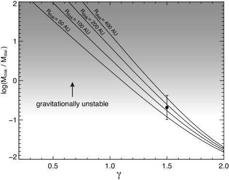
Figure 8.— The inferred disk mass in units of the stellar mass for all the M dwarf multi-transit systems in the Kepler sample as a function of assumed surface density profile index $\gamma$, and disk radius, $R_{\rm disk}$. The data point and error bars show the mean and standard deviation of one such calculation for $\gamma=1.5$ and $R_{\rm disk}=150$ AU to give a sense of the distribution of disk masses derived in each calculation. Disks with masses $\gtrsim 0.2\,M_{\star}$ are expected to be gravitationally unstable.

We also analyze the present-day locations of the Kepler M dwarf planets in terms of the sublimation radius of their host star at 10 Myr of pre-main sequence evolution. We find that between 5 and 14% of the total number of planet candidates fall within the dust sublimation radius of their host stars for large iron grains and $1\,\mu$m silicate grains, respectively, and could not have formed in place.

5.2. Kepler-32 as a Representative of the Kepler M Dwarfs

The Kepler-32 planets span the main distribution of the Kepler M dwarf planets seen in Figure 6 and we plot in Figure 9 the locations of these planets in relation to the full distribution as a function of planet radius and semimajor axis. In both parameter spaces the Kepler-32 planets fall well within the main distribution of planet candidates.

To further explore how representative the Kepler-32 planetary system is of the full sample of Kepler M dwarf planet candidates, we create an ensemble of planetary systems with the Kepler-32 system specifications oriented randomly on the sky with mutual inclinations drawn randomly from a Rayleigh distribution (Lissauer et al. 2011). We find the transit multiplicity fractions are best reproduced with a spread in mutual inclinations of $1.2^{\circ}\pm 0.2^{\circ}$, consistent with values for the entire Kepler planet candidate ensemble ($1.0^{\circ}$–$2.3^{\circ}$; Fabrycky et al. 2012b). The discrepancies between the real and simulated distributions of transiting systems are largest for the single transit systems (55% simulated vs. 73% real). This would be expected for a situation where the typical planetary system contains less than 5 planets or is less compact. However, we note that the observed transit multiplicity of Kepler M dwarf systems can be recreated remarkably well assuming the case that all planetary systems are exact clones of Kepler-32.

Figure 9.— The distributions of Kepler M dwarf planet candidates as a function of planet radius and semimajor axis (blank histogram; not including KOI-254, 256, 531, 1152, 1459, or 1902) in comparison to the Kepler-32 planets (hashed histogram).

The distribution of stellar masses, radii, and metallicities for the Kepler M dwarf sample are shown in Figure 10. A narrow range of stellar mass and radius is seen peaked around 0.5 in solar units due to the magnitude limit of the sample and is shown in contrast to the present day mass function of single stars (PDMF; Chabrier 2003) in the top panel. Kepler-32 is seen to be representative of the full sample in all quantities.

Figure 10.— The distribution of stellar masses and radii for our sample of M dwarf planet host stars are sharply peaked around 0.53 $M_{\odot}$ and 0.51 $R_{\odot}$, respectively. The present day mass function of single field stars in the Galaxy (Chabrier 2003) normalized to the number of stars in our sample is shown as the dotted line in the top panel for reference. Metallicities for our sample fall mostly between $-0.4$ and $0.4$. Kepler-32 values denoted by the vertical dashed line all fall near the center of these distributions.

5.3. Planet Occurrence

The planet occurrence rate for M dwarf planets has been calculated to be about 0.3 for planets with radii $>2$ $R_{\oplus}$ and periods less than 50 days (Mann et al. 2012). However, only 28 planets of the 100 total in our Kepler M dwarf ensemble satisfy these criteria. Therefore the total planet occurrence rate for short period planets around M dwarfs is much higher than this number. The detection of planet signals within the Kepler M dwarf sample is not uniform causing a systematic uncertainty to planet occurrence estimations. Since we have no way to correct for this currently, we ignore this effect which will result in a lower limit of the occurrence rate.

The number of planets per star in our sample is estimated as

$$f=\sum_{i}^{n_{p}}\frac{1}{\sum_{j}^{n_{\star,i}}p_{i,j}}$$ (8)

where $j$ is the index of the sum over all stars around which planet $i$ could be detected, $n_{\star,i}$ (see, e.g., Howard et al. 2012), and

$$p_{i,j}=\frac{R_{\star,j}}{a_{i}}$$ (9)

is the geometric probability of detecting planet $i$ around star $j$ if eccentricity is negligible and $R_{p}/R_{\star}\ll 1$. Since the KIC stellar radii values for stars with $T_{\rm eff}\lesssim 4500$ K are unreliable, we randomly sample the distribution of stellar radii in Figure 10 estimated from near infrared spectra for this calculation. Evaluating Equation 8 over our sample yields $f=1.0\pm 0.1$ planets per star where we use a binomial error estimate.

Though we do not perform statistical validations for all the Kepler M dwarf planets, our sample is expected to have a higher fidelity than the total ensemble of Kepler transit signals since we culled our sample by hand. The planet occurrence derived from our sample assuming 90% fidelity, $f_{90}$, is calculated by evaluating equation 8 repeatedly for 90 randomly drawn planets of the 100 total. We find $f_{90}=0.9\pm 0.1$ where the stated error is the standard deviation of the distribution of 1000 realizations. As a futher check, we limit our sample to the 28 planets with $R_{p}>2$ $R_{\oplus}$ and $P<50$ d to obtain $f=0.26\pm 0.05$ at the lower end of the estimations of Mann et al. (2012). This may be further evidence that our estimations are conservative.

Counting only one planet per system in equation 8 gives the occurrence of stars with at least one planet, $0.51\pm 0.07$ (not including KOI-254), which together with our estimate of the total occurrence gives the average number of planets per system as $\sim 2$. Stars with masses characteristic of the Kepler M dwarf sample are a factor of $\sim 1.8$ times more common than stars of 1 $M_{\odot}$ (Chabrier 2003), and the planets of the Kepler-32 system are representative of the planets that form around these stars. Therefore the insights gleaned from the Kepler-32 system both show us where to look for additional planets in the Solar Neighborhood, and provide a template for understanding the formation of the ubiquitous compact planetary systems throughout the Galaxy.

5.4. Summary and Future Directions

We present a detailed analysis of the Kepler-32 planetary system which offers the rare circumstance of 5 transit signals. While two of the planets have been previously validated through evidence of their mutual gravitational interactions, we validate the remaining three transit signals probabilistically using observations from the W. M. Keck Observatory as constraints. This validation makes Kepler-32 the richest system of transiting planets known around an M dwarf.

Kepler-32 has a markedly compact architecture. All five planets orbit within one third of Mercury’s distance from the Sun, with the closest planet orbiting only 4.3 stellar radii from the Kepler-32 photosphere. The three middle planets lie close to a 1:2:3 period commensurability that is unlikely to be the result of chance.

Our refined stellar parameters improve the derived planetary characteristics, and aid in reconstructing this system’s formation history. Several pieces of evidence from our analyses indicate that the Kepler-32 planets did not form where we see them today:

• the dust sublimation radius of Kepler-32 lying outside the present day semimajor axis of Kepler-32 f for longer than a typical protostellar disk lifetime

• the extremely high surface densities inferred by assuming in situ formation

• the limited range of gravitational influence for planetary embryos located so close to their host star

• the unlikely arrangement of three planets in the system near a 1:2:3 period commensurability

• the high volatile content of Kepler-32 b and c.

This conclusion necessitates planet migration through a disk, and our order of magnitude calculations for the migration rates of the Kepler-32 planets embedded in a typical protostellar disk suggest the presence of gas. If true, this would limit the formation time of the Kepler-32 planets to $\lesssim 10$ Myr—the known timescales over which gaseous disks survive.

Kepler-32 is found to be representative of the full sample of 66 Kepler M dwarf host stars, and the Kepler-32 planets span the mid-line of the distribution of 100 Kepler M dwarf planet candidates in radius-semimajor axis space. Although we are unable to treat each system in this ensemble with the same care as for Kepler-32, we show that similar analyses applied to the ensemble give consistent results to those derived for Kepler-32. Thus the formation scenario deduced from Kepler-32 offers a plausible blueprint for the formation of the full sample of Kepler M dwarf planets.

We select out 4682 M dwarfs from the Kepler Input Catalog that have been observed with Kepler and use their observational parameters to derive the planet occurrence rate of Kepler M dwarf planet candidates. We confirm that within the completeness limits of the first 6 quarters of Kepler data, the M dwarf planet candidates have an occurrence rate about 3 times that of solar-type stars, while the occurrence rate of all candidates around M dwarfs is $1.0\pm 0.1$. We expect the fidelity of our culled sample to be above 90%. Thus the compact systems of planets around the Kepler M dwarf sample are a major population of planets throughout the Galaxy amplifying the significance of the insights gleaned from Kepler-32.

At the time of this writing, there are only 37 planets confirmed to exist around 24 M dwarfs in the Galaxy (exoplanets.org, Wright et al. 2011). The Kepler space telescope has revealed 100 planet candidates around 66 M dwarfs from which we draw our statistics. It would be of great benefit to the study of M dwarf planet formation to explore and validate a larger statistical sample of M dwarfs such that comparisons can be drawn against the detailed analyses of solar-type stars (e.g., Youdin 2011). The continued monitoring of the current sample is also important as this will reveal trends in planet occurrence as a function of orbital period for the smallest planets.

Mass measurements of the growing numbers of confirmed M dwarf planets will also play an important role in interpreting their origins. This can be achieved with nearby M dwarfs using precision radial velocity measurements, or by using alternative techniques such the amplitude of transit timing variations.

Lastly, direct imaging of the inner few AU of nearby protostellar disks will be possible in multiple wavebands with the Atacama Large Telescope Array (ALMA). The modeling of this emission may be the most direct way to constrain where in the protoplanetary disk compact planetary systems form.

References

- Agüeros et al. (2011) Agüeros, M. A., et al. 2011, ApJ, 740, 110
- Andrews & Williams (2007) Andrews, S. M., & Williams, J. P. 2007, ApJ, 659, 705
- Andrews et al. (2009) Andrews, S. M., Wilner, D. J., Hughes, A. M., Qi, C., & Dullemond, C. P. 2009, ApJ, 700, 1502
- Baraffe et al. (1998) Baraffe, I., Chabrier, G., Allard, F., & Hauschildt, P. H. 1998, A&A, 337, 403
- Baranec et al. (2012) Baranec, C., et al. 2012, ArXiv e-prints
- Barnes (2007) Barnes, S. A. 2007, ApJ, 669, 1167
- Barnes (2010) —. 2010, ApJ, 722, 222
- Batalha et al. (2012) Batalha, N. M., et al. 2012, ArXiv e-prints
- Batygin & Morbidelli (2012) Batygin, K., & Morbidelli, A. 2012, ArXiv e-prints
- Bochanski et al. (2010) Bochanski, J. J., Hawley, S. L., Covey, K. R., West, A. A., Reid, I. N., Golimowski, D. A., & Ivezić, Ž. 2010, AJ, 139, 2679
- Borucki et al. (2011a) Borucki, W. J., et al. 2011a, ApJ, 728, 117
- Borucki et al. (2011b) —. 2011b, ApJ, 736, 19
- Bromley & Kenyon (2011) Bromley, B. C., & Kenyon, S. J. 2011, ApJ, 735, 29
- Brown et al. (2011) Brown, T. M., Latham, D. W., Everett, M. E., & Esquerdo, G. A. 2011, AJ, 142, 112
- Cassan et al. (2012) Cassan, A., et al. 2012, Nature, 481, 167
- Chabrier (2003) Chabrier, G. 2003, PASP, 115, 763
- Chambers (1999) Chambers, J. E. 1999, MNRAS, 304, 793
- Chambers & Wetherill (1998) Chambers, J. E., & Wetherill, G. W. 1998, Icarus, 136, 304
- Chambers et al. (1996) Chambers, J. E., Wetherill, G. W., & Boss, A. P. 1996, Icarus, 119, 261
- Chiang & Laughlin (2012) Chiang, E., & Laughlin, G. 2012, ArXiv e-prints
- Cresswell & Nelson (2008) Cresswell, P., & Nelson, R. P. 2008, A&A, 482, 677
- Crida et al. (2006) Crida, A., Morbidelli, A., & Masset, F. 2006, Icarus, 181, 587
- Delfosse et al. (2000) Delfosse, X., Forveille, T., Ségransan, D., Beuzit, J.-L., Udry, S., Perrier, C., & Mayor, M. 2000, A&A, 364, 217
- Eisner (2012) Eisner, J. A. 2012, ApJ, 755, 23
- Fabrycky et al. (2012a) Fabrycky, D. C., et al. 2012a, ApJ, 750, 114
- Fabrycky et al. (2012b) —. 2012b, ArXiv e-prints
- Fortney et al. (2007) Fortney, J. J., Marley, M. S., & Barnes, J. W. 2007, ApJ, 659, 1661
- Gladman (1993) Gladman, B. 1993, Icarus, 106, 247
- Goldreich & Tremaine (1979) Goldreich, P., & Tremaine, S. 1979, ApJ, 233, 857
- Gould et al. (2003) Gould, A., Pepper, J., & DePoy, D. L. 2003, ApJ, 594, 533
- Hansen & Murray (2012) Hansen, B. M. S., & Murray, N. 2012, ApJ, 751, 158
- Hayashi (1981) Hayashi, C. 1981, Progress of Theoretical Physics Supplement, 70, 35
- Hodgkin & Pye (1994) Hodgkin, S. T., & Pye, J. P. 1994, MNRAS, 267, 840
- Howard et al. (2012) Howard, A. W., et al. 2012, ApJS, 201, 15
- Isella et al. (2009) Isella, A., Carpenter, J. M., & Sargent, A. I. 2009, ApJ, 701, 260
- Isella et al. (2006) Isella, A., Testi, L., & Natta, A. 2006, A&A, 451, 951
- Jenkins et al. (2010a) Jenkins, J. M., et al. 2010a, ApJ, 713, L87
- Jenkins et al. (2010b) Jenkins, J. M., et al. 2010b, in Society of Photo-Optical Instrumentation Engineers (SPIE) Conference Series, Vol. 7740, Society of Photo-Optical Instrumentation Engineers (SPIE) Conference Series
- Jester et al. (2005) Jester, S., et al. 2005, AJ, 130, 873
- Johnson et al. (2010a) Johnson, J. A., Aller, K. M., Howard, A. W., & Crepp, J. R. 2010a, PASP, 122, 905
- Johnson et al. (2012) Johnson, J. A., et al. 2012, AJ, 143, 111
- Johnson et al. (2010b) —. 2010b, PASP, 122, 149
- Kasting et al. (1993) Kasting, J. F., Whitmire, D. P., & Reynolds, R. T. 1993, Icarus, 101, 108
- Kennedy & Kenyon (2008) Kennedy, G. M., & Kenyon, S. J. 2008, ApJ, 673, 502
- Kirsh et al. (2009) Kirsh, D. R., Duncan, M., Brasser, R., & Levison, H. F. 2009, Icarus, 199, 197
- Kley & Nelson (2012) Kley, W., & Nelson, R. P. 2012, ArXiv e-prints
- Koch et al. (2010) Koch, D. G., et al. 2010, ApJ, 713, L79
- Kokubo & Ida (1998) Kokubo, E., & Ida, S. 1998, Icarus, 131, 171
- Laughlin et al. (2004) Laughlin, G., Bodenheimer, P., & Adams, F. C. 2004, ApJ, 612, L73
- Lecavelier Des Etangs (2007) Lecavelier Des Etangs, A. 2007, A&A, 461, 1185
- Levison et al. (2007) Levison, H. F., Morbidelli, A., Gomes, R., & Backman, D. 2007, Protostars and Planets V, 669
- Lin & Papaloizou (1979) Lin, D. N. C., & Papaloizou, J. 1979, MNRAS, 186, 799
- Lissauer (1987) Lissauer, J. J. 1987, Icarus, 69, 249
- Lissauer (2007) —. 2007, ApJ, 660, L149
- Lissauer et al. (2012) Lissauer, J. J., et al. 2012, ApJ, 750, 112
- Lissauer et al. (2011) —. 2011, ApJS, 197, 8
- Lithwick & Wu (2012) Lithwick, Y., & Wu, Y. 2012, ApJ, 756, L11
- Lithwick et al. (2012) Lithwick, Y., Xie, J., & Wu, Y. 2012, ArXiv e-prints
- Mann et al. (2012) Mann, A. W., Gaidos, E., Lépine, S., & Hilton, E. J. 2012, ApJ, 753, 90
- Masset et al. (2006) Masset, F. S., D’Angelo, G., & Kley, W. 2006, ApJ, 652, 730
- Moore et al. (2012) Moore, A., Hasan, I., & Quillen, A. 2012, ArXiv e-prints
- Morton (2012) Morton, T. D. 2012, ArXiv e-prints
- Morton & Johnson (2011) Morton, T. D., & Johnson, J. A. 2011, ApJ, 738, 170
- Muirhead et al. (2012a) Muirhead, P. S., Hamren, K., Schlawin, E., Rojas-Ayala, B., Covey, K. R., & Lloyd, J. P. 2012a, ApJ, 750, L37
- Muirhead et al. (2012b) Muirhead, P. S., et al. 2012b, ApJ, 747, 144
- Murray & Dermott (2000) Murray, C. D., & Dermott, S. F. 2000, Solar System Dynamics
- Nidever et al. (2002) Nidever, D. L., Marcy, G. W., Butler, R. P., Fischer, D. A., & Vogt, S. S. 2002, ApJS, 141, 503
- Nutzman & Charbonneau (2008) Nutzman, P., & Charbonneau, D. 2008, PASP, 120, 317
- Pollack et al. (1994) Pollack, J. B., Hollenbach, D., Beckwith, S., Simonelli, D. P., Roush, T., & Fong, W. 1994, ApJ, 421, 615
- Rogers et al. (2011) Rogers, L. A., Bodenheimer, P., Lissauer, J. J., & Seager, S. 2011, ApJ, 738, 59
- Smith & Lissauer (2009) Smith, A. W., & Lissauer, J. J. 2009, Icarus, 201, 381
- Smith et al. (2009) Smith, R. J., Clark, P. C., & Bonnell, I. A. 2009, MNRAS, 396, 830
- Tarter et al. (2007) Tarter, J. C., et al. 2007, Astrobiology, 7, 30
- Vogt et al. (1994) Vogt, S. S., et al. 1994, in Society of Photo-Optical Instrumentation Engineers (SPIE) Conference Series, Vol. 2198, Society of Photo-Optical Instrumentation Engineers (SPIE) Conference Series, ed. D. L. Crawford & E. R. Craine, 362
- Weidenschilling (1977) Weidenschilling, S. J. 1977, Ap&SS, 51, 153
- West et al. (2005) West, A. A., Walkowicz, L. M., & Hawley, S. L. 2005, PASP, 117, 706
- Wetherill (1990) Wetherill, G. W. 1990, Annual Review of Earth and Planetary Sciences, 18, 205
- Williams & Cieza (2011) Williams, J. P., & Cieza, L. A. 2011, ARA&A, 49, 67
- Wright et al. (2011) Wright, J. T., et al. 2011, PASP, 123, 412
- Wu & Lithwick (2012) Wu, Y., & Lithwick, Y. 2012, ArXiv e-prints
- Youdin (2011) Youdin, A. N. 2011, ApJ, 742, 38