Joint Iterative Power Allocation and Linear Interference Suppression Algorithms in Cooperative DS-CDMA Networks

Abstract

This work presents joint iterative power allocation and interference suppression algorithms for spread spectrum networks which employ multiple hops and the amplify-and-forward cooperation strategy for both the uplink and the downlink. We propose a joint constrained optimization framework that considers the allocation of power levels across the relays subject to individual and global power constraints and the design of linear receivers for interference suppression. We derive constrained linear minimum mean-squared error (MMSE) expressions for the parameter vectors that determine the optimal power levels across the relays and the linear receivers. In order to solve the proposed optimization problems, we develop cost-effective algorithms for adaptive joint power allocation, and estimation of the parameters of the receiver and the channels. An analysis of the optimization problem is carried out and shows that the problem can have its convexity enforced by an appropriate choice of the power constraint parameter, which allows the algorithms to avoid problems with local minima. A study of the complexity and the requirements for feedback channels of the proposed algorithms is also included for completeness. Simulation results show that the proposed algorithms obtain significant gains in performance and capacity over existing non-cooperative and cooperative schemes.

I Introduction

Multiple collocated antennas enable the exploitation of the spatial diversity in wireless channels, mitigating the effects of fading and enhancing the performance of wireless communications systems. Due to size and cost it is often impractical to equip mobile terminals or sensor nodes with multiple antennas. However, spatial diversity gains can be obtained when terminals with single antennas establish a distributed antenna array through cooperation [1]-[3]. In a cooperative transmission system, terminals or users relay signals to each other in order to propagate redundant copies of the same signals to the destination user or terminal. To this end, the designer must employ a cooperation strategy such as amplify-and-forward (AF) [3], decode-and-forward (DF) [3, 4] and compress-and-forward (CF) [5].

Prior work on cooperative multiuser direct-sequence code-division multiple-access (DS-CDMA) systems in interference channels has focused on problems that include the impact of multiple access interference (MAI) and intersymbol interference (ISI), the problem of partner selection [4, 10] and the bit error rate (BER) [12, 13], outage performance analysis issues [11], and the evaluation of the spectral efficiency [22] and the diversity gains [23] based on asymptotic results. The main motivation for cooperative relaying with DS-CDMA systems is to increase the capacity, reliability and the interference suppression capability of these networks [10, 11, 22, 23]. Recent contributions in the area of cooperative communications have considered the problem of resource allocation [6, 7] in multi-hop time-division multiple access (TDMA) systems and MIMO systems [8, 9]. Related work on DS-CDMA system has focused on adaptive modulation [14], power and rate allocation [18, 20] and scheduling [21]. In the literature, there has been no attempt to jointly consider the problem of power allocation and interference mitigation in cooperative multiuser DS-CDMA systems so far. This problem is of paramount importance in cooperative wireless ad-hoc and sensor networks [14]-[18] that utilize DS-CDMA systems. These networks require multiple hops to communicate with nodes that are far from the base station in order to increase their coverage [19]. Moreover, multi-hop cooperative relaying can substantially improve the interference suppression capabilities [10, 12, 13].

The goal of this paper is to devise a cross-layer optimization strategy to significantly increase the capacity, reliability and coverage of spread spectrum networks which employ multiple hops and the AF cooperation protocol. Specifically, the problem of joint resource allocation and linear interference suppression in multiuser DS-CDMA with a general number of hops is addressed. In order to facilitate the receiver design, we adopt linear multiuser receivers [24, 25] which only require a training sequence and the timing. More sophisticated receiver techniques [24, 26, 27, 28] are also possible for situations with increased levels of interference. A joint constrained optimization framework that considers the allocation of power levels among the relays subject to individual and global power constraints and the design of linear receivers is presented. It should be noted that the proposed design with individual power constraints has been initially reported in [29], whereas the proposed design with both individual and global power constraints has been introduced in [30]. Here, the proposed designs are described and investigated in further detail, more complete derivations along with analysis and simulations results are included. Linear MMSE expressions that jointly determine the optimal power levels across the relays and the linear receivers are derived. Adaptive least squares (LS) algorithms are also developed for efficiently solving the joint optimization problems and mitigating the effects of MAI and ISI, and allocating the power levels across the links. An analysis of the optimization problem is conducted and shows that the problem can have its convexity enforced by an appropriate selection of the power constraint parameter. This allows the algorithms to avoid problems with local minima. A study of the computational complexity and the requirements for feedback channels of the proposed algorithms is also included.

The main contributions of this work can be summarized as:
1) A joint constrained optimization framework for the allocation of power levels among the relays subject to individual and global power constraints and the design of linear receivers;
2) Constrained linear MMSE expressions for the power allocation and the design of linear receive filters;
3) Recursive algorithms for estimating the channels, the power allocation and the receive filters;
4) Convexity analysis of the proposed optimization problems;
5) A study of the computational complexity and the requirements for feedback channels of the proposed and existing algorithms.

The rest of this paper is organized as follows. Section II describes a cooperative DS-CDMA system model with multiple relays. Section III is devoted to the problem formulation and the constrained linear MMSE design of the interference mitigation receiver and the power allocation. The proposed LS algorithms for the estimation of the receive filter, the power allocation and the channels subject to a global and individual power constraints are developed in Sections IV and V, respectively. Section VI is devoted to the analysis of the computational complexity and feedback requirements of the proposed algorithms. Section VI presents and discusses the simulations and Section VII draws the conclusions.

II Cooperative DS-CDMA System and Data Models

Consider a synchronous DS-CDMA system communicating over multipath channels with QPSK modulation, $K$ users, $N$ chips per symbol and $L$ ($L<N$) as the maximum number of propagation paths for each link. The synchronous DS-CDMA systems is considered for simplicity as it captures most of the effects of asynchronous systems with a low delay spread [25, 26]. We consider both uplink and downlink transmissions. The network is equipped with an AF protocol that allows communication in multiple hops using $n_{r}$ relays in a repetitive fashion. Therefore, we have $n_{p}=n_{r}+1$ phases of transmission or hops and only one transmitter (source or relay) is active per phase, which increases the delay but also improves the coverage. The throughput is affected by the fact that there is an extra time slot per phase of transmission, however, there are situations for which the performance gains can offset the extra time slots and the throughput can be improved. Other cooperation protocols such as DF can be employed without significant modifications, however, the AF has been adopted for simplicity and due to its lower complexity for implementation [3]. We assume that the source node or terminal transmits data organized in packets comprising $P$ symbols, where there is a preamble with training symbols followed by a part with data symbols. We also assume that the packet contains a sufficient number of training symbols in the preamble for parameter estimation and that the network can coordinate transmissions and cooperation. The relays and destination terminals are equipped with linear receivers, which are synchronized with their desired signals. Since the focus of this work is on the resource allocation and linear interference mitigation, we assume perfect synchronization, however, this assumption can be relaxed to account for more realistic synchronization effects in the system. The proposed algorithms for power allocation and interference mitigation are employed at the receivers. A feedback channel is required to convey the power allocation parameters, which should cope with the channel variations.

Figure 1: (a) Uplink and (b) downlink of the cooperative DS-CDMA system.

The cooperative DS-CDMA system under consideration is depicted in Fig. 1. The data model is described for the uplink in what follows. However, it should be remarked that the downlink data models can be obtained as a particular case of the uplink one. The received signals are filtered by a matched filter, sampled at chip rate and organized into $M\times 1$ vectors ${\boldsymbol{r}}_{sd}$, ${\boldsymbol{r}}_{sr_{i}}$ and ${\boldsymbol{r}}_{r_{i}d}$, which describe the signal received from the source to the destination, the source to the relays, and the relays to the destination, respectively,

$$\begin{split}{\boldsymbol{r}}_{sd}&=\sum_{k=1}^{K}a_{sd}^{k}{\boldsymbol{D}}_{k}{\boldsymbol{h}}_{sd,k}b_{k}+{\boldsymbol{\eta}}_{sd}+{\boldsymbol{n}}_{sd},\\ {\boldsymbol{r}}_{sr_{j}}&=\sum_{k=1}^{K}a_{sr_{j}}^{k}{\boldsymbol{D}}_{k}{\boldsymbol{h}}_{sr_{j},k}{b}_{k}+{\boldsymbol{\eta}}_{sr_{j}}+{\boldsymbol{n}}_{sr_{j}},\\ {\boldsymbol{r}}_{r_{j}d}&=\sum_{k=1}^{K}a_{r_{j}d}^{k}{\boldsymbol{D}}_{k}{\boldsymbol{h}}_{r_{j}d,k}\tilde{b}_{k}^{r_{j}d}+{\boldsymbol{\eta}}_{r_{j}d}+{\boldsymbol{n}}_{r_{j}d},\end{split}$$ (1)

where $M=N+L-1$. The quantity $b_{k}[m_{j}]$ corresponds to the transmitted symbol of user $k$, whereas $\tilde{b}_{k}^{r_{j}d}$ represents the symbol $b_{k}^{r_{j}d}$ processed at the relay $j$ using the AF protocol. The amplitudes of the source to the destination, the source to the relay $j$ and the relay $j$ to the destination links for user $k$ are denoted by $a_{sd}^{k}$, $a_{sr_{j}}^{k}$ and $a_{r_{j}d}^{k}$, respectively. The vectors ${\boldsymbol{n}}_{sd}$, ${\boldsymbol{n}}_{sr_{j}}$ and ${\boldsymbol{n}}_{r_{j}d}$ represent the noise at the receiver of the destination and the relays. The vectors ${\boldsymbol{\eta}}_{sd}$, ${\boldsymbol{\eta}}_{sr_{j}}$ and ${\boldsymbol{\eta}}_{r_{j}d}$ denote the intersymbol interference (ISI) arising from the source to destination, source to relay $j$ and relay $j$ to destination links, respectively. The $M\times L$ matrix ${\boldsymbol{D}}_{k}$ has the signature sequences of each user shifted down by one position at each column that form

$${\boldsymbol{D}}_{k}=\left[\begin{array}[]{c c c }d_{k}(1)&&{\bf 0}\\ \vdots&\ddots&d_{k}(1)\\ d_{k}(N)&&\vdots\\ {\bf 0}&\ddots&d_{k}(N)\\ \end{array}\right],$$ (2)

where ${\boldsymbol{d}}_{k}=\big{[}d_{k}(1),~{}d_{k}(2),~{}\ldots,~{}d_{k}(N)\big{]}$ stands for the signature sequence of user $k$, the $L\times 1$ channel vectors from the source to the destination, the source to the relay, and the relay to the destination are ${\boldsymbol{h}}_{sd,k}$, ${\boldsymbol{h}}_{r_{j}d,k}$, ${\boldsymbol{h}}_{r_{j}s,k}$, respectively. By stacking the data vectors in (1) (including the links from the relays to the destination) into a $(n_{r}+1)M\times 1$ received vector at the destination we have

$$\begin{split}\left[\begin{array}[]{l}{\boldsymbol{r}}_{sd}\\ {\boldsymbol{r}}_{r_{1}d}\\ \vdots\\ {\boldsymbol{r}}_{r_{n_{r}}d}\end{array}\right]&=\left[\begin{array}[]{l}\sum_{k=1}^{K}a_{sd}^{k}{\boldsymbol{D}}_{k}{\boldsymbol{h}}_{sd,k}b_{k}\\ \sum_{k=1}^{K}a_{{r_{1}}d}^{k}{\boldsymbol{D}}_{k}{\boldsymbol{h}}_{{r_{1}}d,k}{\tilde{b}}_{k}^{{r_{1}}d}\\ \vdots\\ \sum_{k=1}^{K}a_{{r_{n_{r}}}d}^{k}{\boldsymbol{D}}_{k}{\boldsymbol{h}}_{r_{n_{r}}d,k}{\tilde{b}}_{k}^{{r_{n_{r}}}d}\end{array}\right]+\left[\begin{array}[]{l}{\boldsymbol{\eta}}_{sd}\\ {\boldsymbol{\eta}}_{r_{1}d}\\ \vdots\\ {\boldsymbol{\eta}}_{r_{n_{r}}d}\end{array}\right]+\left[\begin{array}[]{l}{\boldsymbol{n}}_{sd}\\ {\boldsymbol{n}}_{r_{1}d}\\ \vdots\\ {\boldsymbol{n}}_{r_{n_{r}}d}\end{array}\right]\end{split}$$ (3)

By using the stacked received data from the source and the relays for joint processing and using $i$ to denote the desired symbol in the transmitted packet and its received and relayed copies, we can rewrite the data in a compact form given by

$${\boldsymbol{r}}[i]=\sum_{k=1}^{K}{\boldsymbol{\mathcal{C}}}_{k}{\boldsymbol{\mathcal{H}}}_{k}[i]{\boldsymbol{B}}_{k}[i]{\boldsymbol{a}}_{k}[i]+{\boldsymbol{\eta}}[i]+{\boldsymbol{n}}[i],$$ (4)

where the $(n_{r}+1)M\times(n_{r}+1)L$ matrix ${\boldsymbol{\mathcal{C}}}_{k}$ contains shifted versions of ${\boldsymbol{D}}_{k}$ as shown by

$${\boldsymbol{\mathcal{C}}}_{k}=\left[\begin{array}[]{c c c c}{\boldsymbol{D}}_{k}&{\bf 0}&\ldots&{\bf 0}\\ {\bf 0}&{\boldsymbol{D}}_{k}&\ldots&\vdots\\ \vdots&\vdots&\ddots&{\bf 0}\\ {\bf 0}&{\bf 0}&\ldots&{\boldsymbol{D}}_{k}\\ \end{array}\right].$$ (5)

The $(n_{r}+1)L\times(n_{r}+1)$ matrix ${\boldsymbol{\mathcal{H}}}_{k}[i]$ has the channel gains of the links between the source and the destination, and the relays and the destination. The $(n_{r}+1)\times(n_{r}+1)$ diagonal matrix ${\boldsymbol{B}}_{k}[i]={\rm diag}(b_{k}~{}{\tilde{b}}_{k}^{{r_{1}}d}\ldots{\tilde{b}}_{k}^{{r_{n}}d})$ contains the symbols transmitted from the source to the destination ($b_{k}$) and the $n_{r}$ symbols transmitted from the relays to the destination (${\tilde{b}}_{k}^{{r_{1}}d}\ldots{\tilde{b}}_{k}^{{r_{n}}d}$) on the main diagonal, the $(n_{r}+1)\times 1$ vector ${\boldsymbol{a}}_{k}[i]=[a_{sd}^{k}~{}a_{{r_{1}}d}^{k}\ldots a_{{r_{n_{r}}}d}^{k}]^{T}$ of the amplitudes, the $(n_{r}+1)M\times 1$ vector ${\boldsymbol{\eta}}[i]$ with the ISI terms and $(n_{r}+1)M\times 1$ vector ${\boldsymbol{n}}[i]$ with the noise. A schematic that summarizes the transmission and reception schemes is depicted in Fig. 2.

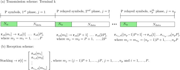
Figure 2: (a) Transmission and (b) reception scheme of the cooperative DS-CDMA system.

III Problem Statement and Proposed MMSE Design

This section states the problem of joint power allocation and interference suppression for a cooperative DS-CDMA network. Specifically, constrained optimization problems are formulated in order to describe the joint power allocation and interference suppression problems subject to a global and individual power constraints. The proposed linear MMSE designs are aimed at the destination, which is responsible for jointly computing the receiver parameters and the power allocation that is sent via a feedback channel to the source.

III-A MMSE Design with a Global Power Constraint

The linear MMSE design of the power allocation of the links across the source, relay and destination terminals and interference suppression filters is presented here using a global power constraint. Let us express the received vector in (4) in a more convenient way for the proposed optimization. The $(n_{r}+1)M\times 1$ received vector can be written as

$${\boldsymbol{r}}[i]={\boldsymbol{\mathcal{C}}}_{T}{\boldsymbol{\mathcal{H}}}_{T}[i]{\boldsymbol{B}}_{T}[i]{\boldsymbol{a}}_{T}[i]+{\boldsymbol{\eta}}[i]+{\boldsymbol{n}}[i],$$ (6)

where the $(n_{r}+1)M\times K(n_{r}+1)L$ matrix ${\boldsymbol{\mathcal{C}}}_{T}=[{\boldsymbol{\mathcal{C}}}_{1}~{}{\boldsymbol{\mathcal{C}}}_{2}~{}\ldots~{}{\boldsymbol{\mathcal{C}}}_{K}]$ contains all the signatures, the $K(n_{r}+1)L\times K(n_{r}+1)$ matrix ${\boldsymbol{\mathcal{H}}}_{T}[i]$ contains the channel gains of all the links, the $K(n_{r}+1)\times K(n_{r}+1)$ diagonal matrix ${\boldsymbol{B}}_{T}[i]={\rm diag}(b_{1}[m_{1}]~{}{\tilde{b}}_{1}^{{r_{1}}d}[m_{2}]\ldots{\tilde{b}}_{1}^{{r_{n_{r}}}d}[m_{n_{p}}]\ldots b_{K}[m_{1}]~{}{\tilde{b}}_{K}^{{r_{1}}d}[m_{2}]\ldots{\tilde{b}}_{K}^{{r_{n_{r}}}d}[m_{n_{p}}])$ contains the symbols transmitted from all the sources to the destination and from all the relays to the destination on the main diagonal, and the $K(n_{r}+1)\times 1$ power allocation vector ${\boldsymbol{a}}_{T}[i]=[a_{sd}^{1}[m_{1}]~{}a_{{r_{1}}d}^{1}[m_{2}]\ldots a_{{r_{n_{r}}}d}^{1}[m_{n_{p}}]\ldots a_{sd}^{K}[m_{1}]~{}a_{{r_{1}}d}^{K}[m_{2}]\ldots a_{{r_{n_{r}}}d}^{K}[m_{n_{p}}]]^{T}$ contains the amplitudes of all the links.

Consider a joint MMSE design of the receivers for the $K$ users represented by a $(n_{r}+1)M\times K$ parameter matrix ${\boldsymbol{W}}[i]=[{\boldsymbol{w}}_{1}[i],~{}\ldots,~{}{\boldsymbol{w}}_{K}[i]]$ and for the computation of the $K(n_{r}+1)\times 1$ optimal power allocation vector ${\boldsymbol{a}}_{T,{\rm opt}}[i]$. This problem can be cast as

$$\begin{split}[{\boldsymbol{W}}_{{\rm opt}},{\boldsymbol{a}}_{T,{\rm opt}}]&=\arg\min_{{\boldsymbol{W}}[i],{\boldsymbol{a}}_{k}[i]}~{}E[||{\boldsymbol{b}}[i]-{\boldsymbol{W}}^{H}[i]{\boldsymbol{r}}[i]||^{2}]\\ {\rm subject~{}to~{}}&{\boldsymbol{a}}_{T}^{H}[i]{\boldsymbol{a}}_{T}[i]=P_{T},\end{split}$$ (7)

where the $K\times 1$ vector ${\boldsymbol{b}}[i]=[b_{1}[i],~{}\ldots,b_{K}[i]]^{T}$ represents the desired symbols of the $K$ users. The linear MMSE expressions for the parameter matrix ${\boldsymbol{W}}_{\rm opt}$ and the vector ${\boldsymbol{a}}_{T,{\rm opt}}$ can be obtained by transforming the above constrained optimization problem into an unconstrained one with the method of Lagrange multipliers [39] which leads to

$$\begin{split}{\mathcal{L}}_{T}&=E\big{[}\big{\|}{\boldsymbol{b}}[i]-{\boldsymbol{W}}^{H}[i]\big{(}{\boldsymbol{\mathcal{C}}}_{T}{\boldsymbol{\mathcal{H}}}_{T}[i]{\boldsymbol{B}}_{T}[i]{\boldsymbol{a}}_{T}[i]+{\boldsymbol{\eta}}[i]+{\boldsymbol{n}}[i]\big{)}\big{\|}^{2}\big{]}\\ &\quad+\lambda_{T}({\boldsymbol{a}}_{T}^{H}[i]{\boldsymbol{a}}_{T}[i]-P_{T}),\end{split}$$ (8)

Fixing ${\boldsymbol{a}}_{T}[i]$, taking the gradient terms of the Lagrangian and equating them to zero yields

$${\boldsymbol{W}}_{{\rm opt}}={\boldsymbol{R}}^{-1}{\boldsymbol{P}}_{{\boldsymbol{\mathcal{C}}}{\boldsymbol{\mathcal{H}}}},$$ (9)

where the covariance matrix of the received vector is ${\boldsymbol{R}}=E[{\boldsymbol{r}}[i]{\boldsymbol{r}}^{H}[i]]={\boldsymbol{\mathcal{C}}}_{T}{\boldsymbol{\mathcal{H}}}_{T}[i]{\boldsymbol{B}}_{T}[i]{\boldsymbol{a}}_{T}[i]{\boldsymbol{a}}_{T}^{H}[i]{\boldsymbol{B}}_{T}^{H}[i]{\boldsymbol{\mathcal{H}}}^{H}_{T}[i]{\boldsymbol{\mathcal{C}}}_{T}^{H}+\sigma^{2}{\boldsymbol{I}}$ and ${\boldsymbol{P}}_{{\boldsymbol{\mathcal{C}}}{\boldsymbol{\mathcal{H}}}}=E[{\boldsymbol{r}}[i]{\boldsymbol{b}}^{H}[i]]=E[{\boldsymbol{\mathcal{C}}}_{T}{\boldsymbol{\mathcal{H}}}_{T}[i]{\boldsymbol{B}}_{T}[i]{\boldsymbol{a}}_{T}[i]{\boldsymbol{b}}^{H}[i]]$ is the $(n_{r}+1)M\times K$ cross-correlation matrix. The matrices ${\boldsymbol{R}}$ and ${\boldsymbol{P}}_{{\boldsymbol{\mathcal{C}}}{\boldsymbol{\mathcal{H}}}}$ depend on the power allocation vector ${\boldsymbol{a}}_{T}[i]$. The expression for ${\boldsymbol{a}}_{T}[i]$ is obtained by fixing ${\boldsymbol{W}}[i]$, taking the gradient terms of the Lagrangian and equating them to zero which leads to

$${\boldsymbol{a}}_{T,{\rm opt}}=({\boldsymbol{R}}_{{\boldsymbol{a}}_{T}}+\lambda_{T}{\boldsymbol{I}})^{-1}{\boldsymbol{p}}_{{\boldsymbol{a}}_{T}},$$ (10)

where the $K(n_{r}+1)\times K(n_{r}+1)$ covariance matrix ${\boldsymbol{R}}_{{\boldsymbol{a}}_{T}}=E[{\boldsymbol{\boldsymbol{B}}}_{T}^{H}[i]{\boldsymbol{\mathcal{H}}}^{H}_{T}[i]{\boldsymbol{\mathcal{C}}}_{T}^{H}{\boldsymbol{W}}[i]{\boldsymbol{W}}^{H}[i]{\boldsymbol{\mathcal{C}}}_{T}{\boldsymbol{\mathcal{H}}}_{T}[i]{\boldsymbol{B}}_{T}[i]]$ and the vector ${\boldsymbol{p}}_{{\boldsymbol{a}}_{T}}=E[{\boldsymbol{B}}_{T}^{H}[i]{\boldsymbol{\mathcal{H}}}_{T}[i]^{H}{\boldsymbol{\mathcal{C}}}_{T}^{H}{\boldsymbol{W}}[i]{\boldsymbol{b}}[i]]$ is a $K(n_{r}+1)\times 1$ cross-correlation vector. The Lagrange multiplier $\lambda_{T}$ in the expression above plays the role of a regularization term and has to be determined numerically due to the difficulty of evaluating its expression. The expressions in (9) and (10) depend on each other and require the estimation of the channel matrix ${\boldsymbol{\mathcal{H}}}_{T}[i]$. Thus, it is necessary to estimate the channel and to iterate (9) and (10) with initial values to obtain a solution. In addition, the network has to convey all the information necessary to compute the global power allocation including the filter ${\boldsymbol{W}}_{{\rm opt}}$. The expressions in (9) and (10) require matrix inversions with cubic complexity ( $O((n_{r}+1)M)^{3})$ and $O((K(n_{r}+1))^{3})$, should be iterated as they depend on each other and require channel estimation.

III-B MMSE Design with Individual Power Constraints

Here, the joint design of a linear MMSE receiver and the calculation of the optimal power levels across the relays subject to individual power constraints is presented. Consider an MMSE approach for the design of the receive filter ${\boldsymbol{w}}_{k}[i]$ and the power allocation vector ${\boldsymbol{a}}_{k}[i]$ for user $k$. This design problem is posed as

$$\begin{split}[{\boldsymbol{w}}_{k,{\rm opt}},{\boldsymbol{a}}_{k,{\rm opt}}]&=\arg\min_{{\boldsymbol{w}}_{k}[i],{\boldsymbol{a}}_{k}[i]}~{}E[|b_{k}[i]-{\boldsymbol{w}}_{k}^{H}[i]{\boldsymbol{r}}[i]|^{2}]\\ {\rm subject~{}to~{}}&{\boldsymbol{a}}_{k}^{H}[i]{\boldsymbol{a}}_{k}[i]=P_{A,k},~{}~{}~{}k=1,~{}2,~{}\ldots,~{}K.\end{split}$$ (11)

The expressions for the parameter vectors ${\boldsymbol{w}}_{k}[i]$ and ${\boldsymbol{a}}_{k}[i]$ can be obtained by transforming the above constrained optimization problem into an unconstrained one with the method of Lagrange multipliers [39], which leads to

$$\begin{split}{\mathcal{L}}_{k}&=E\big{[}\big{|}b_{k}[i]-{\boldsymbol{w}}_{k}^{H}[i]\big{(}\sum_{l=1}^{K}{\boldsymbol{\mathcal{C}}}_{l}{\boldsymbol{\mathcal{H}}}_{l}[i]{\boldsymbol{B}}_{l}[i]{\boldsymbol{a}}_{l}[i]+{\boldsymbol{\eta}}[i]+{\boldsymbol{n}}[i]\big{)}\big{|}^{2}\big{]}\\ &\quad+\lambda_{k}({\boldsymbol{a}}_{k}^{H}[i]{\boldsymbol{a}}_{k}[i]-P_{A,k}),~{}~{}~{}k=1,~{}2,~{}\ldots,~{}K.\end{split}$$ (12)

Fixing ${\boldsymbol{a}}_{k}[i]$, taking the gradient terms of the Lagrangian and equating them to zero yields

$${\boldsymbol{w}}_{k,{\rm opt}}={\boldsymbol{R}}^{-1}{\boldsymbol{p}}_{{\boldsymbol{\mathcal{C}}}{\boldsymbol{\mathcal{H}}}},~{}~{}~{}k=1,~{}2,~{}\ldots,~{}K,$$ (13)

where ${\boldsymbol{R}}=\sum_{k=1}^{K}{\boldsymbol{\mathcal{C}}}_{k}{\boldsymbol{\mathcal{H}}}_{k}[i]{\boldsymbol{B}}_{k}[i]{\boldsymbol{a}}_{k}[i]{\boldsymbol{a}}_{k}^{H}[i]{\boldsymbol{B}}_{k}^{H}[i]{\boldsymbol{\mathcal{H}}}^{H}_{k}[i]{\boldsymbol{\mathcal{C}}}_{k}^{H}+\sigma^{2}{\boldsymbol{I}}$ is the covariance matrix and ${\boldsymbol{p}}_{{\boldsymbol{\mathcal{C}}}{\boldsymbol{\mathcal{H}}}}=E[b_{k}^{*}[i]{\boldsymbol{r}}[i]]={\boldsymbol{\mathcal{C}}}_{k}{\boldsymbol{\mathcal{H}}}[i]{\boldsymbol{a}}_{k}[i]$ is the cross-correlation vector. The quantities ${\boldsymbol{R}}$ and ${\boldsymbol{p}}_{{\boldsymbol{\mathcal{C}}}{\boldsymbol{\mathcal{H}}}}$ depend on ${\boldsymbol{a}}_{k}[i]$. By fixing ${\boldsymbol{w}}_{k}[i]$, the expression for ${\boldsymbol{a}}_{k}[i]$ is given by

$${\boldsymbol{a}}_{k,{\rm opt}}=({\boldsymbol{R}}_{{\boldsymbol{a}}_{k}}+\lambda_{k}{\boldsymbol{I}})^{-1}{\boldsymbol{p}}_{{\boldsymbol{a}}_{k}},~{}~{}~{}k=1,~{}2,~{}\ldots,~{}K,$$ (14)

where ${\boldsymbol{R}}_{{\boldsymbol{a}}_{k}}=\sum_{k=1}^{K}{\boldsymbol{\boldsymbol{B}}}_{k}^{H}[i]{\boldsymbol{\mathcal{H}}}^{H}_{k}[i]{\boldsymbol{\mathcal{C}}}_{k}^{H}{\boldsymbol{w}}_{k}[i]{\boldsymbol{w}}_{k}^{H}[i]{\boldsymbol{\mathcal{C}}}_{k}{\boldsymbol{\mathcal{H}}}_{k}[i]{\boldsymbol{B}}_{k}[i]$ is the $(n_{r}+1)\times(n_{r}+1)$ covariance matrix and the $(n_{r}+1)\times 1$ cross-correlation vector is ${\boldsymbol{p}}_{{\boldsymbol{a}}_{k}}=E[b_{k}[i]{\boldsymbol{B}}_{k}^{H}[i]{\boldsymbol{\mathcal{H}}}_{k}[i]^{H}{\boldsymbol{\mathcal{C}}}_{k}^{H}{\boldsymbol{w}}_{k}[i]]$. The expressions in (13) and (14) have to be iterated as they depend on each other and require the estimation of the channel matrices ${\boldsymbol{\mathcal{H}}}_{k}[i]$. The expressions in (13) and (14) also require matrix inversions with cubic complexity ( $O(((n_{r}+1)M)^{3})$ and $O((n_{r}+1)^{3})$. In what follows, we will develop adaptive algorithms for computing ${\boldsymbol{a}}_{k,{\rm opt}}$, ${\boldsymbol{w}}_{k,{\rm opt}}$ and the channels ${\boldsymbol{\mathcal{H}}}_{k}[i]$ for $k=1,\ldots,K$ in an alternating fashion.

IV Proposed Joint Estimation Algorithms with a Global Power Constraint

Here we present adaptive joint estimation algorithms to determine the parameters of the linear receiver, the power allocation and the channel with a global power constraint. The proposed joint power allocation and interference suppression (JPAIS) algorithms with a global power constraint (GPC) are simply called JPAIS-GPC, are suitable for the uplink of DS-CDMA systems and rely on LS-based estimation algorithms. The proposed algorithms are based on the idea of alternating optimization [31, 32], in which the recursions for computing the parameters of interest are employed in cycles of iterations and over the received symbols. Note that more advanced algorithms [33]-[38] could also be considered in this context.

IV-A Receiver and Power Allocation Parameter Estimation Algorithms

Let us now consider the following proposed least squares (LS) optimization problem

$$\begin{split}[\hat{\boldsymbol{W}}[i],\hat{\boldsymbol{a}}_{T}[i]]&=\arg\min_{{\boldsymbol{W}}[i],{\boldsymbol{a}}_{T}[i]}~{}\sum_{l=1}^{i}\alpha^{i-l}||{\boldsymbol{b}}[l]-{\boldsymbol{W}}^{H}[i]{\boldsymbol{r}}[l]||^{2}\\ {\rm subject~{}to~{}}&{\boldsymbol{a}}_{T}^{H}[i]{\boldsymbol{a}}_{T}[i]=P_{T},\end{split}$$ (15)

where $\alpha$ is a forgetting factor. The goal is to develop a cost-effective recursive solution to (15). To this end, we will resort to the theory of adaptive algorithms [39] and derive a constrained joint iterative recursive least squares (RLS) algorithm. This algorithm will compute $\hat{\boldsymbol{W}}[i]$ and $\hat{\boldsymbol{a}}_{T}[i]$ and will exchange information between the recursions. The part of the algorithm to compute $\hat{\boldsymbol{W}}[i]$ uses ${\boldsymbol{\Phi}}[i]=\hat{\boldsymbol{R}}[i]=\sum_{l=1}^{i}\alpha^{l=i}{\boldsymbol{r}}[l]{\boldsymbol{r}}^{H}[l]$ and is given by

$${\boldsymbol{k}}[i]=\frac{\alpha^{-1}{\boldsymbol{\Phi}}[i]{\boldsymbol{r}}[i]}{1+\alpha^{-1}{\boldsymbol{r}}^{H}[i]{\boldsymbol{\Phi}}[i]{\boldsymbol{r}}[i]},$$ (16)

$${\boldsymbol{\Phi}}[i]=\alpha^{-1}{\boldsymbol{\Phi}}[i-1]-\alpha^{-1}{\boldsymbol{k}}[i]{\boldsymbol{r}}^{H}[i]{\boldsymbol{\Phi}}[i-1],$$ (17)

$$\hat{\boldsymbol{W}}[i]=\hat{\boldsymbol{W}}[i-1]+{\boldsymbol{k}}[i]{\boldsymbol{\xi}}^{H}[i],$$ (18)

where the a priori estimation error is given by

$${\boldsymbol{\xi}}[i]={\boldsymbol{b}}[i]-\hat{\boldsymbol{W}}^{H}[i-1]{\boldsymbol{r}}[i].$$ (19)

The derivation for the recursion that estimates the power allocation $\hat{\boldsymbol{a}}_{T}[i]$ presents a difficulty related to the enforcement of the constraint and how to incorporate it into an efficient LS algorithm. This is because the problem in (15) incorporates a Lagrange multiplier ($\lambda_{T}$) to ensure the global power constraint and the resulting system of equations cannot be solved with the aid of the matrix inversion lemma [39] due to its structure. Our approach is to obtain a recursive expression by relaxing the constraint, to solve the system of equations with Gaussian elimination or with an adaptive conjugate gradient algorithm [41], and then ensure the constraint is incorporated via a subsequent normalization procedure.

The power allocation vector ${\boldsymbol{a}}_{T}[i]$ is estimated via the solution of the following equation

$$\hat{\boldsymbol{R}}_{\hat{\boldsymbol{a}}_{T}}[i]\hat{\boldsymbol{a}}_{T}[i]=\hat{\boldsymbol{p}}_{\boldsymbol{a}_{T}}[i],$$ (20)

where the $K(n_{r}+1)\times K(n_{r}+1)$ input data correlation matrix is given by

$$\begin{split}\hat{\boldsymbol{R}}_{\boldsymbol{a}_{T}}[i]&=\alpha\hat{\boldsymbol{R}}_{\boldsymbol{a}_{T}}[i-1]+{\boldsymbol{U}}_{T}[i]{\boldsymbol{U}}_{T}^{H}[i],\end{split}$$ (21)

where the $K(n_{r}+1)\times K$ matrix ${\boldsymbol{U}}_{T}[i]={\boldsymbol{\boldsymbol{B}}}_{T}^{H}[l]\hat{\boldsymbol{\mathcal{H}}}^{H}_{T}[l]{\boldsymbol{\mathcal{C}}}_{T}^{H}\hat{\boldsymbol{W}}[i]$ and the $K(n_{r}+1)\times 1$ cross-correlation vector is given by

$$\begin{split}\hat{\boldsymbol{p}}_{\boldsymbol{a}_{T}}[i]&=\hat{\boldsymbol{p}}_{\boldsymbol{a}_{T}}[i-1]+{\boldsymbol{U}}_{T}[i]{\boldsymbol{b}}[i].\end{split}$$ (22)

The system of linear equations in (20) can be solved via Gaussian elimination with cubic complexity or more efficiently with quadratic complexity via an adaptive conjugate gradient algorithm [41] as described below

$${\boldsymbol{v}}[i]=\hat{\boldsymbol{p}}_{\boldsymbol{a}_{T}}[i]-\hat{\boldsymbol{R}}_{\hat{\boldsymbol{a}}_{T}}[i]\hat{\boldsymbol{a}}_{T}[i],~{}~{}{\boldsymbol{d}}[i]={\boldsymbol{v}}[i],$$ (23)

$$\alpha[i]={\boldsymbol{v}}^{H}[i]{\boldsymbol{v}}[i]/({\boldsymbol{d}}^{H}[i]\hat{\boldsymbol{R}}_{\hat{\boldsymbol{a}}_{T}}[i]{\boldsymbol{d}}[i],$$ (24)

$$\hat{\boldsymbol{a}}_{T}[i+1]=\hat{\boldsymbol{a}}_{T}[i]+\alpha[i]\hat{\boldsymbol{R}}_{\hat{\boldsymbol{a}}_{T}}[i]{\boldsymbol{d}}[i],$$ (25)

$${\boldsymbol{v}}[i+1]={\boldsymbol{v}}[i]-\alpha[i]\hat{\boldsymbol{R}}_{\hat{\boldsymbol{a}}_{T}}[i]{\boldsymbol{d}}[i],$$ (26)

$$\beta[i+1]={\boldsymbol{v}}^{H}[i+1]{\boldsymbol{v}}[i+1]/({\boldsymbol{v}}^{H}[i]{\boldsymbol{v}}[i]),$$ (27)

$${\boldsymbol{d}}[i+1]={\boldsymbol{v}}[i+1]+\beta[i+1]{\boldsymbol{d}}[i],$$ (28)

In order to ensure the global power constraint $\hat{\boldsymbol{a}}_{T}^{H}[i]\hat{\boldsymbol{a}}_{T}[i]=P_{T}$, we apply the following rule

$$\hat{\boldsymbol{a}}_{T}[i]\leftarrow\sqrt{P_{T}}~{}\hat{\boldsymbol{a}}_{T}[i]\big{(}\sqrt{\hat{\boldsymbol{a}}_{T}^{H}[i]\hat{\boldsymbol{a}}_{T}[i]}\big{)}^{-1}.$$ (29)

The algorithms for recursive computation of $\hat{\boldsymbol{W}}[i]$ and $\hat{\boldsymbol{a}}_{T}[i]$ require estimates of the channel vector ${\boldsymbol{\mathcal{H}}}_{T}[i]$, which will also be developed in what follows. The complexity of the proposed algorithm is $O(((n_{r}+1)M)^{2})$ for calculating $\hat{\boldsymbol{W}}[i]$ and $O((K(n_{r}+1))^{2})$ for obtaining $\hat{\boldsymbol{a}}_{T}[i]$.

IV-B Channel Estimation with a Global Power Constraint

We present a channel estimator that considers jointly all the $K$ users and exploits the knowledge of the receive filter matrix $\hat{\boldsymbol{W}}[i]$ and the power allocation vector $\hat{\boldsymbol{a}}_{T}[i]$. Let us consider the received vector in (6) and develop a channel estimation algorithm for ${\boldsymbol{\mathcal{H}}}_{T}[i]$. The proposed channel estimator can be derived from the following optimization problem

$$\begin{split}\hat{\boldsymbol{\mathcal{H}}}_{T}[i]&=\arg\min_{{\boldsymbol{\mathcal{H}}}_{T}[i]}~{}\sum_{l=1}^{i}\alpha^{i-l}||{\boldsymbol{r}}[l]-{\boldsymbol{\mathcal{C}}}_{T}{\boldsymbol{\mathcal{H}}}_{T}[i]{\boldsymbol{B}}_{T}[i]{\boldsymbol{a}}_{T}[i]||^{2}.\end{split}$$ (30)

The solution to the above optimization problem is given by

$$\hat{\boldsymbol{H}}_{T}[i]=\big{(}{\boldsymbol{\mathcal{C}}}_{T}^{H}{\boldsymbol{\mathcal{C}}}_{T}\big{)}^{-1}\hat{\boldsymbol{P}}_{{\boldsymbol{\mathcal{H}}}_{T}}^{-1}[i]\hat{\boldsymbol{R}}_{{\boldsymbol{\mathcal{H}}}_{T}}^{-1}[i],$$ (31)

where the matrix inversion $\big{(}{\boldsymbol{\mathcal{C}}}_{T}^{H}{\boldsymbol{\mathcal{C}}}_{T}\big{)}^{-1}$ can be pre-computed and stored at the terminal of interest, and the $K(n_{r}+1)L\times(n_{r}+1)L$ correlation matrix $\hat{\boldsymbol{P}}_{{\boldsymbol{\mathcal{H}}}_{T}}[i]$ is computed by the formula

$$\begin{split}\hat{\boldsymbol{P}}_{{\boldsymbol{\mathcal{H}}}_{T}}[i]&=\sum_{l=1}^{i}\alpha^{i-l}{\boldsymbol{\mathcal{C}}}_{T}^{H}{\boldsymbol{r}}[l]{\boldsymbol{u}}_{{\boldsymbol{\mathcal{H}}}_{T}}^{H}[l]\\ &=\hat{\boldsymbol{P}}_{{\boldsymbol{\mathcal{H}}}_{T}}[i-1]+{\boldsymbol{\mathcal{C}}}_{T}^{H}{\boldsymbol{r}}[i]{\boldsymbol{u}}_{{\boldsymbol{\mathcal{H}}}_{T}}^{H}[i],\end{split}$$ (32)

where the $K(n_{r}+1)L\times 1$ input data vector ${\boldsymbol{u}}_{{\boldsymbol{\mathcal{H}}}_{T}}[i]$ for this recursion is

$${\boldsymbol{u}}_{{\boldsymbol{\mathcal{H}}}_{T}}[i]={{\boldsymbol{B}}}_{T}[i]{\boldsymbol{a}}_{T}[i],$$ (33)

and the inverse of the $K(n_{r}+1)L\times K(n_{r}+1)L$ matrix $\hat{\boldsymbol{R}}_{{\boldsymbol{\mathcal{H}}}_{T}}[i]=\sum_{l=1}^{i}\lambda^{i-l}{\boldsymbol{u}}_{{\boldsymbol{\mathcal{H}}}_{T}}[l]{\boldsymbol{u}}_{{\boldsymbol{\mathcal{H}}}_{T}}^{H}[l]$ is computed with the aid of the matrix inversion lemma [39] as follows

$$\hat{\boldsymbol{R}}_{{\boldsymbol{\mathcal{H}}}_{T}}^{-1}[i]=\frac{\hat{\boldsymbol{R}}_{{\boldsymbol{\mathcal{H}}}_{T}}^{-1}[i-1]}{\alpha}-\frac{\alpha^{-2}\hat{\boldsymbol{R}}_{{h}_{k}}^{-1}[i-1]{\boldsymbol{u}}_{{\boldsymbol{\mathcal{H}}}_{T}}[i]{\boldsymbol{u}}_{{\boldsymbol{\mathcal{H}}}_{T}}^{H}[i]\hat{\boldsymbol{R}}_{{\boldsymbol{\mathcal{H}}}_{T}}^{-1}[i-1]}{1+\alpha^{-1}{\boldsymbol{u}}_{{\boldsymbol{\mathcal{H}}}_{T}}^{H}[i]\hat{\boldsymbol{R}}_{{\boldsymbol{\mathcal{H}}}_{T}}^{-1}[i-1]{\boldsymbol{u}}_{{\boldsymbol{\mathcal{H}}}_{T}}[i]},$$ (34)

This algorithm jointly estimates the coefficients of the channels across all the links and for all users subject to a global power constraint. Therefore, the complexity of the proposed RLS channel estimation algorithm is $O((K(n_{r}+1)L)^{2})$. A summary of the main steps of the GPAIS-GPC algorithms is provided in Table I.

TABLE I: Summary of the JPAIS-GPC.

1. Initialise parameters: $\hat{\boldsymbol{W}}[0]$, $\hat{\boldsymbol{a}}_{T}[0]$ and $\lambda$.

for $i=1,\ldots,P$ do

2. Compute the receive filter $\hat{\boldsymbol{W}}[i]$ using (18).

3. Calculate the power allocation vector $\hat{\boldsymbol{a}}_{T}[i]$ using (25).

4. Normalise $\hat{\boldsymbol{a}}_{T}[i]$ with (29).

5. Compute the channel estimate $\hat{\boldsymbol{H}}_{T}[i]$ using (31).

end for.

6. Transmit power allocation $\hat{\boldsymbol{a}}_{T}[i]$ to users.

V Proposed Joint Estimation Algorithms with Individual Power Constraints

In this section, we present adaptive joint estimation algorithms to determine the parameters of the linear receiver, the power allocation and the channel subject to individual power constraints. The proposed JPAIS algorithms with individual power constraints (IPC) are simply called JPAIS-IPC and, unlike the algorithms presented in the previous section, are more appropriate for the downlink and for distributed resource allocation, detection and estimation. Specifically, the JPAIS-IPC algorithms can be employed in a distributed fashion in which the linear receivers compute the individual receive filter, the power allocation and channel parameters, and then convey the power allocation parameters to the base station.

V-A Receiver and Power Allocation Parameter Estimation

We develop a recursive solution to the expressions in (13) and (14) using time averages instead of the expected value. The proposed RLS algorithms will compute $\hat{\boldsymbol{w}}_{k}[i]$ and $\hat{\boldsymbol{a}}_{k}[i]$ for each user $k$ and will exchange information between the recursions. We fix $\hat{\boldsymbol{a}}_{k}[i]$ and compute the inverse of $\hat{\boldsymbol{R}}[i]$ using the matrix inversion lemma [39] to obtain $\hat{\boldsymbol{w}}_{k}[i]$. Defining ${\boldsymbol{\Phi}}[i]=\hat{\boldsymbol{R}}[i]$ then we can obtain the recursions

$${\boldsymbol{k}}[i]=\frac{\alpha^{-1}{\boldsymbol{\Phi}}[i]{\boldsymbol{r}}[i]}{1+\alpha^{-1}{\boldsymbol{r}}^{H}[i]{\boldsymbol{\Phi}}[i]{\boldsymbol{r}}[i]},$$ (35)

$${\boldsymbol{\Phi}}[i]=\alpha^{-1}{\boldsymbol{\Phi}}[i-1]-\alpha^{-1}{\boldsymbol{k}}[i]{\boldsymbol{r}}^{H}[i]{\boldsymbol{\Phi}}[i-1],$$ (36)

$$\hat{\boldsymbol{w}}_{k}[i]=\hat{\boldsymbol{w}}_{k}[i-1]+{\boldsymbol{k}}[i]\xi^{*}_{k}[i],$$ (37)

where the a priori estimation error is

$$\xi_{k}[i]=b_{k}[i]-{\boldsymbol{w}}_{k}^{H}[i-1]{\boldsymbol{r}}[i].$$ (38)

The derivation for the recursion that estimates the power allocation requires a strategy to enforce the constraint on the individual power of user $k$, which circumvents the need to compute the Lagrange multiplier $\lambda_{k}$. In order to develop the recursions for $\hat{\boldsymbol{a}}_{k}[i]$, we need to compute the inverse of $\hat{\boldsymbol{R}}_{\boldsymbol{a}_{k}}[i]=\sum_{l=1}^{i}{\boldsymbol{\boldsymbol{B}}}_{k}^{H}[l]\hat{\boldsymbol{\mathcal{H}}}^{H}_{k}[l]{\boldsymbol{\mathcal{C}}}_{k}^{H}\hat{\boldsymbol{w}}_{k}[l]\hat{\boldsymbol{w}}^{H}_{k}[l]{\boldsymbol{\mathcal{C}}}_{k}\hat{\boldsymbol{\mathcal{H}}}_{k}[l]{\boldsymbol{B}}_{k}[l]$. To this end, let us first define ${\boldsymbol{\Phi}}_{\boldsymbol{a}_{k}}=\hat{\boldsymbol{R}}_{\boldsymbol{a}_{k}}[i]$ and proceed as follows:

$${\boldsymbol{k}}_{\boldsymbol{a}_{k}}[i]=\frac{\alpha^{-1}{\boldsymbol{\Phi}}_{\boldsymbol{a}_{k}}[i]{\boldsymbol{B}}_{k}^{H}[i]\hat{\boldsymbol{\mathcal{H}}}^{H}_{k}[i]{\boldsymbol{\mathcal{C}}}_{k}^{H}\hat{\boldsymbol{w}}_{k}[i]}{1+\alpha^{-1}\hat{\boldsymbol{w}}_{k}^{H}[i]{\boldsymbol{\mathcal{C}}}_{k}\hat{\boldsymbol{\mathcal{H}}}_{k}[i]{\boldsymbol{B}}_{k}[i]{\boldsymbol{\Phi}}_{\boldsymbol{a}_{k}}[i]{\boldsymbol{B}}_{k}^{H}[i]\hat{\boldsymbol{\mathcal{H}}}^{H}_{k}[i]{\boldsymbol{\mathcal{C}}}_{k}^{H}\hat{\boldsymbol{w}}_{k}[i]},$$ (39)

$${\boldsymbol{\Phi}}_{\boldsymbol{a}_{k}}[i]=\alpha^{-1}{\boldsymbol{\Phi}}_{\boldsymbol{a}_{k}}[i-1]-\alpha^{-1}{\boldsymbol{k}}_{\boldsymbol{a}_{k}}[i]\hat{\boldsymbol{w}}_{k}^{H}[i]{\boldsymbol{\mathcal{C}}}_{k}\hat{\boldsymbol{\mathcal{H}}}_{k}[i]{\boldsymbol{B}}_{k}[i]{\boldsymbol{\Phi}}_{\boldsymbol{a}_{k}}[i-1],$$ (40)

$$\hat{\boldsymbol{a}}_{k}[i]=\hat{\boldsymbol{a}}_{k}[i]+{\boldsymbol{k}}_{\boldsymbol{a}_{k}}[i]\xi_{\boldsymbol{a}_{k}}^{*}[i],$$ (41)

where the a priori estimation error for the above recursion is

$$\xi_{\boldsymbol{a}_{k}}[i]=b_{k}[i]-\hat{\boldsymbol{a}}_{k}^{H}[i]{\boldsymbol{B}}_{k}^{H}[i]\hat{\boldsymbol{\mathcal{H}}}^{H}_{k}[i]{\boldsymbol{\mathcal{C}}}_{k}^{H}\hat{\boldsymbol{w}}_{k}[i],$$ (42)

In order to ensure the individual power constraint ${\boldsymbol{a}}_{k}^{H}[i]{\boldsymbol{a}}_{k}[i]=P_{A,k}$, we apply the rule

$$\hat{\boldsymbol{a}}_{k}[i]\leftarrow\sqrt{P_{A,k}}~{}\hat{\boldsymbol{a}}_{k}[i]\big{(}\sqrt{\hat{\boldsymbol{a}}_{k}^{H}[i]\hat{\boldsymbol{a}}_{k}[i]}\big{)}^{-1}.$$ (43)

The algorithms for recursive computation of $\hat{\boldsymbol{w}}_{k}[i]$ and $\hat{\boldsymbol{a}}_{k}[i]$ require estimates of the channel vector ${\boldsymbol{\mathcal{H}}}_{k}[i]$, which will also be developed in what follows. The complexity of the proposed algorithm is $O(((n_{r}+1)M)^{2})$ for calculating $\hat{\boldsymbol{w}}_{k}[i]$ and $O((n_{r}+1)^{2})$ for obtaining $\hat{\boldsymbol{a}}_{k}[i]$.

V-B Channel Estimation with Individual Power Constraints

We propose here an algorithm that estimates the channels for each user $k$ across all links subject to individual power constraints and exploits the knowledge of the receiver filter $\hat{\boldsymbol{w}}_{k}[i]$ and the power allocation vector $\hat{\boldsymbol{a}}_{k}[i]$. Let us consider the received vector in (4) for the channel estimation procedure. A channel estimation algorithm can be developed to solve the following optimization problem

$$\begin{split}\hat{\boldsymbol{\mathcal{H}}}_{k}[i]&=\arg\min_{{\boldsymbol{\mathcal{H}}}_{k}[i]}~{}\sum_{l=1}^{i}\alpha^{i-l}||{\boldsymbol{r}}[l]-{\boldsymbol{\mathcal{C}}}_{k}{\boldsymbol{\mathcal{H}}}_{k}[i]{\boldsymbol{B}}_{k}[l]{\boldsymbol{a}}_{k}[l]||^{2},\\ ~{}~{}{\rm for}~{}~{}k&=1,~{}2,~{}\ldots,K,\end{split}$$ (44)

The solution to the above optimization problem is

$$\hat{\boldsymbol{\mathcal{H}}}_{k}[i]=\big{(}{\boldsymbol{\mathcal{C}}}_{k}^{H}{\boldsymbol{\mathcal{C}}}_{k}\big{)}^{-1}\hat{\boldsymbol{P}}_{{\boldsymbol{h}}_{k}}[i]\hat{\boldsymbol{R}}_{{\boldsymbol{h}}_{k}}^{-1}[i],~{}~{}{\rm for}~{}~{}k=1,~{}2,~{}\ldots,K,$$ (45)

where the matrix inversion $\big{(}{\boldsymbol{\mathcal{C}}}_{k}^{H}{\boldsymbol{\mathcal{C}}}_{k}\big{)}^{-1}$ can be pre-computed and stored at the base station, relays and mobile terminals, and the $(n_{r}+1)L\times(n_{r}+1)L$ correlation matrix $\hat{\boldsymbol{P}}_{{\boldsymbol{h}}_{k}}[i]$ is computed by the formula

$$\begin{split}\hat{\boldsymbol{P}}_{{\boldsymbol{h}}_{k}}[i]&=\sum_{l=1}^{i}\alpha^{i-l}{\boldsymbol{\mathcal{C}}}_{k}^{H}{\boldsymbol{r}}[l]{\boldsymbol{u}}_{{\boldsymbol{h}}_{k}}^{H}[l]\\ &=\hat{\boldsymbol{P}}_{{\boldsymbol{h}}_{k}}[i-1]+{\boldsymbol{\mathcal{C}}}_{k}^{H}{\boldsymbol{r}}[i]{\boldsymbol{u}}_{{\boldsymbol{h}}_{k}}^{H}[i],\end{split}$$ (46)

where the $(n_{r}+1)L\times 1$ input data vector ${\boldsymbol{u}}_{{\boldsymbol{h}}_{k}}[i]$ for this recursion is

$${\boldsymbol{u}}_{{\boldsymbol{h}}_{k}}[i]={{\boldsymbol{B}}}_{k}[i]{\boldsymbol{a}}_{k}[i]$$ (47)

and the inverse of the $(n_{r}+1)L\times(n_{r}+1)L$ matrix $\hat{\boldsymbol{R}}_{{\boldsymbol{h}}_{k}}^{-1}[i]$ is computed as follows

$$\hat{\boldsymbol{R}}_{{\boldsymbol{h}}_{k}}^{-1}[i]=\alpha^{-1}\hat{\boldsymbol{R}}_{{\boldsymbol{h}}_{k}}^{-1}[i-1]-\frac{\alpha^{-2}\hat{\boldsymbol{R}}_{{h}_{k}}^{-1}[i-1]{\boldsymbol{u}}_{{\boldsymbol{h}}_{k}}[i]{\boldsymbol{u}}_{{\boldsymbol{h}}_{k}}^{H}[i]\hat{\boldsymbol{R}}_{{\boldsymbol{h}}_{k}}^{-1}[i-1]}{1+\alpha^{-1}{\boldsymbol{u}}_{{\boldsymbol{h}}_{k}}^{H}[i]\hat{\boldsymbol{R}}_{{\boldsymbol{h}}_{k}}^{-1}[i-1]{\boldsymbol{u}}_{{\boldsymbol{h}}_{k}}[i]}.$$ (48)

This algorithm estimates the coefficients of the channels of each user $k$ across all the links subject to individual power constraints. The complexity is $O(((n_{r}+1)L)^{2})$. A summary of the main steps of the GPAIS-IPC algorithms is provided in Table I.

TABLE II: Summary of the JPAIS-IPC.

1. Initialise parameters: $\hat{\boldsymbol{w}}_{k}[0]$, $\hat{\boldsymbol{a}}_{k}[0]$ and $\lambda$.

for each user $k$ do

for $i=1,\ldots,P$ do

2. Compute the receive filter $\hat{\boldsymbol{w}}_{k}[i]$ using (37).

3. Calculate the power allocation vector $\hat{\boldsymbol{a}}_{k}[i]$ using (41).

4. Normalise $\hat{\boldsymbol{a}}_{k}[i]$ with (43).

5. Compute the channel estimate $\hat{\boldsymbol{H}}_{k}[i]$ using (45).

end for with variable $i$.

6. Transmit power allocation $\hat{\boldsymbol{a}}_{k}[i]$ to base station.

VI Analysis and Requirements of the Algorithms

In this section, we analyze the optimization problems described in Section III, and assess the requirements of the proposed JPAIS-GPC and JPAIS-IPC algorithms in terms of computational complexity and number of feedback bits.

VI-A Analysis of the Optimization Problems

In this part, we develop an analysis of the optimization problems introduced in Section III, which can be extended to the algorithms introduced in Sections IV and V. Our approach is based on an algebraic manipulation of the original problem and the incorporation of the power constraints to illustrate the properties of the problem. The optimization problems considered in Section III constitute non-convex problems, however, it turns out that it is possible to devise a strategy that modifies the MSE-based optimization and enforces the convexity. This is corroborated by our studies that verify that the algorithms converge to the same solutions regardless of the initialization when this strategy is adopted.

Let us consider the proposed optimization method in (7) and examine the cost function

$$\begin{split}{\mathcal{C}}({\boldsymbol{W}}[i],{\boldsymbol{a}}_{k}[i])&=E[||{\boldsymbol{b}}[i]-{\boldsymbol{W}}^{H}[i]{\boldsymbol{r}}[i]||^{2}]\\ &=E[\sum_{k=1}^{K}|{b}_{k}[i]-[{\boldsymbol{W}}]_{k}^{H}{\boldsymbol{r}}[i]|^{2}],\end{split}$$ (49)

which must be minimized subject to ${\boldsymbol{a}}_{T}^{H}[i]{\boldsymbol{a}}_{T}[i]=P_{T}$ and where $[{\boldsymbol{W}}]_{k}[i]$ denotes the $k$-column of the matrix ${\boldsymbol{W}}[i]$. Let us now express ${\boldsymbol{x}}[i]={\boldsymbol{W}}^{H}[i]{\boldsymbol{r}}[i]$ as

$$\begin{split}{\boldsymbol{x}}[i]&={\boldsymbol{W}}^{H}[i]{\boldsymbol{r}}[i]\\ &={\boldsymbol{W}}^{H}[i](\underbrace{{\boldsymbol{\mathcal{C}}}_{T}{\boldsymbol{\mathcal{H}}}_{T}[i]{\boldsymbol{B}}_{T}[i]}_{{\boldsymbol{\Re}}[i]}{\boldsymbol{a}}_{T}[i]+{\boldsymbol{W}}^{H}[i](\underbrace{{\boldsymbol{\eta}}[i]+{\boldsymbol{n}}[i]}_{{\boldsymbol{t}}[i]})\\ &=\sum_{k=1}^{K}(\underbrace{[{\boldsymbol{W}}]_{k}^{H}[i]{\boldsymbol{\Re}}[i]{\boldsymbol{a}}_{T}[i]+[{\boldsymbol{W}}]_{k}^{H}[i]{\boldsymbol{t}}[i]}_{x_{k}[i]}){\boldsymbol{\pi}}_{k},\end{split}$$ (50)

where ${\boldsymbol{\pi}}_{k}$ is a $K\times 1$ vector that contains a $1$ in the $k$-th position and zeros elsewhere. Now let us consider the joint optimization problem via a single parameter vector defined as

$${\boldsymbol{q}}_{k}[i]=\left[\begin{array}[]{c}[{\boldsymbol{W}}]_{k}[i]\\ {\boldsymbol{a}}_{T}^{*}[i]\end{array}\right].$$ (51)

Using the above definition, we can rewrite the data symbol expression for user $k$ as follows

$$\begin{split}x_{k}[i]&=\sum_{k=1}^{K}\big{(}{\boldsymbol{q}}_{k}^{H}[i]({\boldsymbol{U}}_{s}[i]+{\boldsymbol{U}}_{I}[i]){\boldsymbol{q}}_{k}[i]\big{)}{\boldsymbol{\pi}}_{k}\\ &=\sum_{k=1}^{K}{\boldsymbol{q}}_{k}^{H}[i]{\boldsymbol{U}}_{T}[i]{\boldsymbol{q}}_{k}[i]{\boldsymbol{\pi}}_{k},\end{split}$$ (52)

where the $(n_{r}+1)(M+K)\times(n_{r}+1)(M+K)$ matrices with the signal and noise components are
${\boldsymbol{U}}_{s}[i]=\left[\begin{array}[]{cc}{\boldsymbol{0}}_{(n_{r}+1)K\times(n_{r}+1)K}&{\boldsymbol{0}}_{(n_{r}+1)M\times(n_{r}+1)M}\\ {\boldsymbol{\Re}}[i]&{\boldsymbol{0}}_{(n_{r}+1)K\times(n_{r}+1)K}\end{array}\right]$ and
${\boldsymbol{U}}_{I}[i]=\left[\begin{array}[]{cc}{\boldsymbol{t}}[i]&{\boldsymbol{0}}_{(n_{r}+1)M\times(n_{r}+1)(K+M)-1}\\ {\boldsymbol{0}}_{(n_{r}+1)K\times 1}&{\boldsymbol{0}}_{(n_{r}+1)K\times(n_{r}+1)(K+M)-1}\end{array}\right]$.

If we now rewrite the cost function in (49) as a function of ${\boldsymbol{q}}_{k}[i]$, we obtain the equivalent function

$${\mathcal{C}}({\boldsymbol{q}}_{k}[i])=E[\sum_{k=1}^{K}|{b}_{k}[i]-{\boldsymbol{q}}_{k}[i]^{H}{\boldsymbol{U}}_{T}[i]{\boldsymbol{q}}_{k}[i]|^{2}],$$ (53)

which is also subject to the global power constraint ${\boldsymbol{a}}_{T}^{H}[i]{\boldsymbol{a}}_{T}[i]=P_{T}$. In order to evaluate the convexity of the optimization problem, we can verify if the Hessian (${\boldsymbol{H}}_{k}$) with respect to user $k$ of ${\mathcal{C}}({\boldsymbol{q}}_{k}[i])$ is positive semi-definite if ${\boldsymbol{m}}^{H}{\boldsymbol{H}}_{k}{\boldsymbol{m}}\geq 0$ for all nonzero ${\boldsymbol{m}}\in\boldsymbol{C}^{(n_{r}+1)(M+K)\times 1}$ [41, 40]. Computing the Hessian [41] of the above cost function for the $k$th user we obtain

$$\begin{split}{\boldsymbol{H}}_{k}&=\frac{\partial}{\partial{\boldsymbol{q}}_{k}^{H}[i]}\frac{\partial{\mathcal{C}}({\boldsymbol{q}}_{k}[i])}{\partial{\boldsymbol{q}}_{k}^{H}[i]}\\ &=E\big{[}({\boldsymbol{q}}^{H}_{k}[i]{\boldsymbol{U}}_{T}[i]{\boldsymbol{q}}_{k}[i]-b_{k}^{*}[i]){\boldsymbol{U}}_{T}[i]+{\boldsymbol{U}}^{H}_{T}[i]{\boldsymbol{q}}_{k}[i]{\boldsymbol{q}}_{k}^{H}[i]{\boldsymbol{U}}_{T}[i]\\ &\quad+({\boldsymbol{q}}^{H}_{k}[i]{\boldsymbol{U}}_{T}[i]{\boldsymbol{q}}_{k}[i]-b_{k}[i]){\boldsymbol{U}}^{H}_{T}[i]+{\boldsymbol{U}}_{T}[i]{\boldsymbol{q}}_{k}[i]{\boldsymbol{q}}_{k}^{H}[i]{\boldsymbol{U}}^{H}_{T}[i]\big{]},\end{split}$$ (54)

By examining ${\boldsymbol{H}}_{k}$, we verify that the second and fourth terms are positive semi-definite, whereas the first and the third terms are indefinite. At this stage, it is of central importance in the analysis to employ the constraint ${\boldsymbol{a}}_{T}^{H}[i]{\boldsymbol{a}}_{T}[i]=P_{T}$ and perform some algebraic manipulations in the first and the third terms, which yield

$$\begin{split}&2\Re e\big{\{}E\big{[}\big{(}[{\boldsymbol{W}}]_{k}^{H}[i]{\boldsymbol{\Re}}[i]{\boldsymbol{\beta}}_{T}[i]P_{T}+[{\boldsymbol{W}}]_{k}^{H}[i]{\boldsymbol{t}}[i]-b_{k}^{*}[i]\big{)}{\boldsymbol{U}}_{T}[i]\big{]}\big{\}},\end{split}$$ (55)

where ${\boldsymbol{\beta}}_{T}[i]=({\boldsymbol{a}}_{T}{\boldsymbol{a}}_{T}^{H}[i])^{{\dagger}}{\boldsymbol{a}}_{T}$, $(\cdot)^{{\dagger}}$ represents the pseudo-inverse and the operator $\Re e\{\cdot\}$ selects the real part of the argument. The above development shows that the optimization problem can have its convexity enforced by adjusting the power constraint $P_{T}$ so that the following condition holds

$$\begin{split}P_{T}\geq\frac{{\boldsymbol{m}}^{H}\Re e\big{\{}E\big{[}\big{(}b_{k}^{*}[i]-[{\boldsymbol{W}}]_{k}^{H}[i]{\boldsymbol{t}}[i]\big{)}{\boldsymbol{U}}_{T}[i]\big{]}\big{\}}{\boldsymbol{m}}}{{\boldsymbol{m}}^{H}\Re e\big{\{}E\big{[}\big{(}[{\boldsymbol{W}}]_{k}^{H}[i]{\boldsymbol{\Re}}[i]{\boldsymbol{\beta}}_{T}[i]\big{)}{\boldsymbol{U}}_{T}[i]\big{]}\big{\}}{\boldsymbol{m}}}.\end{split}$$ (56)

The previous analysis can be conducted for the proposed JPAIS-IPC algorithm and leads to the following condition

$$\begin{split}P_{k}\geq\frac{{\boldsymbol{m}}^{H}\Re e\big{\{}E\big{[}\big{(}b_{k}^{*}[i]-{\boldsymbol{w}}_{k}^{H}[i]{\boldsymbol{j}}[i]\big{)}{\boldsymbol{U}}_{T}[i]\big{]}\big{\}}{\boldsymbol{m}}}{{\boldsymbol{m}}^{H}\Re e\big{\{}E\big{[}\big{(}{\boldsymbol{w}}_{k}^{H}[i]{\boldsymbol{\Re}}_{k}[i]{\boldsymbol{\gamma}}_{k}[i]\big{)}{\boldsymbol{U}}_{T}[i]\big{]}\big{\}}{\boldsymbol{m}}},\end{split}$$ (57)

where ${\boldsymbol{\Re}}_{k}[i]={\boldsymbol{\mathcal{C}}}_{k}{\boldsymbol{\mathcal{H}}}_{k}[i]{\boldsymbol{B}}_{k}[i]$, ${\boldsymbol{U}}_{k+j}[i]={\boldsymbol{U}}_{k}[i]+{\boldsymbol{U}}_{j}[i]$, ${\boldsymbol{U}}_{k}[i]=\left[\begin{array}[]{cc}{\boldsymbol{0}}_{(n_{r}+1)\times(n_{r}+1)}&{\boldsymbol{0}}_{(n_{r}+1)M\times(n_{r}+1)M}\\ {\boldsymbol{\Re}}_{k}[i]&{\boldsymbol{0}}_{(n_{r}+1)\times(n_{r}+1)}\end{array}\right]$ and
${\boldsymbol{U}}_{j}[i]=\left[\begin{array}[]{cc}{\boldsymbol{j}}[i]&{\boldsymbol{0}}_{(n_{r}+1)M\times(n_{r}+1)M-1}\\ {\boldsymbol{0}}_{(n_{r}+1)\times 1}&{\boldsymbol{0}}_{(n_{r}+1)\times(n_{r}+1)M-1}\end{array}\right]$, the $(n_{r}+1)M\times 1$ vector ${\boldsymbol{j}}[i]=\sum_{l\neq k}^{K}{\boldsymbol{\mathcal{C}}}_{l}{\boldsymbol{\mathcal{H}}}_{l}[i]{\boldsymbol{B}}_{l}[i]+{\boldsymbol{\eta}}[i]+{\boldsymbol{n}}[i]$, and ${\boldsymbol{\gamma}}_{k}[i]=({\boldsymbol{a}}_{k}{\boldsymbol{a}}_{k}^{H}[i])^{{\dagger}}{\boldsymbol{a}}_{k}$. These conditions have been verified by numerical experiments, which corroborate the analytical results. Therefore, the optimization problem can have its convexity enforced by an appropriate selection of the global and individual power constraints $P_{T}$ and $P_{k}$, respectively.

VI-B Computational Complexity Requirements

We discuss here the computational complexity of the proposed and existing algorithms. Specifically, we will detail the required number of complex additions and multiplications of the proposed JPAIS-GPC and JPAIS-IPC algorithms, and compare them with interference suppression schemes without cooperation (NCIS) and with cooperation (CIS) [10, 11] using an equal power allocation across the relays. Both uplink and downlink scenarios are considered in the analysis. In Table III we show the computational complexity required by each recursion associated with a parameter vector/matrix for the JPAIS-GPC, which is more suitable for the uplink.

TABLE III: Computational complexity of algorithms with a global power constraint .

	Number of operations per symbol
Parameter	Additions	Multiplications
	$2((n_{r}+1)M)^{2}$	$3((n_{r}+1)M)^{2}$
$\hat{\boldsymbol{W}}[i]$	$+2K((n_{r}+1)M)$	$+2K((n_{r}+1)M)$
	$-(n_{r}+1)M+1$	$+3(n_{r}+1)M+1$
	$3K(K(n_{r}+1))$	$K(K(n_{r}+1))$
	$+K(n_{r}+1)(L-1)$	$+4(K(n_{r}+1))^{2}$
$\hat{\boldsymbol{a}}_{T}[i]$	$+K(M(n_{r}+1))$	$+(K+L)(K(n_{r}+1))^{2}$
	$+K(K(n_{r}+1))$	$-(K(n_{r}+1))^{2}$
	$+6(K(n_{r}+1))^{2}$	$+K(M(n_{r}+1)L$
	$+3K(n_{r}+1)+n_{r}+2$	$+n_{r}$
	$5(K(n_{r}+1)L)^{2}$	$+5(K(n_{r}+1))^{2}$
$\hat{\boldsymbol{H}}_{T}[i]$	$+5K(n_{r}+1)L$	$+6K(n_{r}+1)L$
	$+3$	$+1$

TABLE IV: Computational complexity of algorithms with individual power constraints.

	Number of operations per symbol
Parameter	Additions	Multiplications
	$2((n_{r}+1)M)^{2}$	$3((n_{r}+1)M)^{2}$
$\hat{\boldsymbol{w}}_{k}[i]$	$+(n_{r}+1)M$	$+5(n_{r}+1)M$
	$+1$	$+1$
	$2(n_{r}+1)^{2}$	$3(n_{r}+1)^{2}$
	$+3(n_{r}+1)$	$+7(n_{r}+1)$
$\hat{\boldsymbol{a}}_{k}[i]$	$+M(n_{r}+1)L$	$+M(n_{r}+1)L$
	$+(n_{r}+1)L$	$+(n_{r}+1)L$
	$-3$	$+3$
	$2((n_{r}+1)L)^{2}$	$6((n_{r}+1)L)^{2}$
$\hat{\boldsymbol{H}}_{k}[i]$	$+5M(n_{r}+1)L$	$+M(n_{r}+1)L$
	$-5(n_{r}+1)+3$	$+4(n_{r}+1)+1$

In Table IV we describe the computational complexity required by each recursion associated with a parameter vector for the JPAIS-IPC algorithm, which is suitable for both the uplink and the downlink. A noticeable difference between the JPAIS-GPC and the JPAIS-IPC is that the latter is employed for each user, whereas the former is used for all the $K$ users in the system. Since the computation of the inverse of $\hat{\boldsymbol{R}}[i]$ is common to all users for the uplink in our system, the JPAIS-GPC is more efficient than the JPAIS-IPC when the latter is computed for all the $K$ users.

TABLE V: Computational complexity of the proposed JPAIS and existing algorithms.

Algorithm	Recursions
JPAIS-GPC (Uplink)	$\hat{\boldsymbol{W}}[i]$, $\hat{\boldsymbol{a}}_{T}[i]$,$\hat{\boldsymbol{H}}_{T}[i]$
JPAIS-IPC (Downlink)	$\hat{\boldsymbol{w}}_{k}[i]$, $\hat{\boldsymbol{a}}_{k}[i]$, $\hat{\boldsymbol{H}}_{k}[i]$
CIS (Uplink)	$\hat{\boldsymbol{W}}[i]$, $\hat{\boldsymbol{a}}_{T}[i]$ is fixed
CIS (Downlink)	$\hat{\boldsymbol{w}}_{k}[i]$, $\hat{\boldsymbol{a}}_{k}[i]$ is fixed
NCIS (Uplink)	$\hat{\boldsymbol{W}}[i]$ with $n_{r}=0$
NCIS (Downlink)	$\hat{\boldsymbol{w}}_{k}[i]$ with $n_{r}=0$

The recursions employed for the proposed JPAIS-GPC and the JPAIS-IPC are general and parts of them are used in the existing CIS and NIS algorithms. Therefore, we can use them to describe the required computational complexity of the existing algorithms. In Table V we show the required recursions for the proposed and existing algorithms, whose complexity is detailed in Tables III and IV.

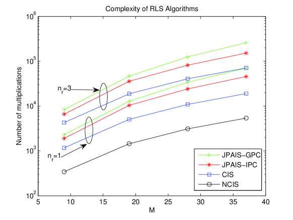
Figure 3: Computational complexity in terms of the number of complex multiplications of the proposed and existing schemes for the uplink.

In Fig. 3, we illustrate the required computational complexity for the proposed and existing schemes for different number of relays ($n_{r}$). The curves show that the proposed JPAIS-GPC and JPAIS-IPC are more complex than the CIS scheme and the NCIS. This is due to the fact that the power allocation and channel estimation recursions are employed. However, we will show in the next section that this additional required complexity (which is modest and equivalent to an additional $20-25\%$ cost as compared to the CIS scheme) can significantly improve the performance of the system.

VI-C Feedback Channel Requirements

The proposed JPAIS algorithms require feedback signalling in order to allocate the power levels across the relays. In order to illustrate how these requirements are addressed, we can refer to Fig. 4 which depicts the structure for both the data and feedback packets. The data packet comprises a preamble with a number of training symbols ($N_{\rm tr}$), which are used for parameter estimation and synchronization, and the transmitted data symbols ($N_{\rm data}$). The feedback packet requires the transmission of the power allocation vector ${\boldsymbol{a}}_{T}$ for the case of the JPAIS-GPC algorithm, whereas it requires the transmission of ${\boldsymbol{a}}_{k}$ for each user for JPAIS-IPC. A typical number of bits $n_{b}$ required to quantize each coefficient of the vectors ${\boldsymbol{a}}_{T}$ and ${\boldsymbol{a}}_{k}$ via scalar quantization is $n_{b}=4$ bits. More efficient schemes employing vector quantization [42, 43] and that take into account correlations between the coefficients are also possible.

For the uplink (or multiple-access channel), the base station (or access point) needs to feedback the power levels across the links to the $K$ destination users in the system. With the JPAIS-GPC algorithm, the parameter vector ${\boldsymbol{a}}_{T}$ with $(n_{r}+1)Kn_{b}$ bits/packet must be broadcasted to the $K$ users. For the JPAIS-IPC algorithm, a parameter vector ${\boldsymbol{a}}_{k}$ with $(n_{r}+1)n_{b}$ bits/packet must be broadcasted to each user in the system. In terms of feedback, the JPAIS-IPC algorithm is more flexible and may require less feedback bits if there is no need for a constant update of the power levels for all $K$ users.

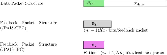
Figure 4: Proposed structure of the data and feedback packets.

For the downlink (or broadcast channel), the $K$ users must feedback the power levels across the links to the base station. With the JPAIS-GPC algorithm, the parameter vector ${\boldsymbol{a}}_{T}$ with $(n_{r}+1)Kn_{b}$ bits/packet must be computed by each user and transmitted to the base station, which uses the ${\boldsymbol{a}}_{T}$ vector coming from each user. An algorithm for data fusion or a simple averaging procedure can be used. For the JPAIS-IPC algorithm, a parameter vector ${\boldsymbol{a}}_{k}$ with $(n_{r}+1)n_{b}$ bits/packet must be transmitted from each user to the base station. In terms of feedback, the JPAIS-IPC algorithm requires significantly less feedback bits than the JPAIS-GPC in this scenario.

VII Simulations

In this section, a simulation study of the proposed JPAIS and existing algorithms is carried out. The first existing scheme that is considered in the comparisons is a linear interference suppression technique that only takes into account the source to destination links and does not consider the contribution of the relays. This scheme is denoted non-cooperative interference suppression (NCIS) and corresponds to a linear receive filter designed according to the MMSE criterion or computed with an RLS algorithm for each user. The second existing scheme is denoted cooperative interference suppression (CIS) and processes the signals arriving from the source and the relays using an equal power allocation across the relays for each user. The CIS scheme employs a linear receive filter designed according to the MMSE criterion or adjusted with an RLS algorithm, and the entries of the power allocation parameter vectors are equal (equal power allocation). We first evaluate the bit error ratio (BER) performance of the proposed JPAIS-GPC and JPAIS-IPC algorithms and compare them with the NCIS and the CIS schemes. We consider a DS-CDMA system with randomly generated spreading codes with a processing gain $N=16$. The noise samples at the receivers of the relays and the destination are drawn from zero mean complex Gaussian random variables with variance $\sigma^{2}$. The fading channels (that can be time-varying or time-invariant) are generated using a random power delay profile with gains taken from a complex Gaussian variable with unit variance and mean zero, $L=3$ paths spaced by one chip, and are normalized for unit power. The time-varying channels are generated according to Clarke’s model [44], which is parameterized by the normalized Doppler frequency $f_{d}T$, where $f_{d}$ is the Doppler frequency and $T$ is the inverse of the symbol rate. The power constraint parameter $P_{A,k}$ is set for each user so that one can control the SNR (${\rm SNR}=P_{A,k}/\sigma^{2}$) and $P_{T}=KP_{A,k}$, whereas the power distribution of the interferers follows a log-normal distribution with associated standard deviation of $3$ dB. We adopt the AF cooperative strategy with repetitions and all the relays and the destination terminal are equipped with linear MMSE or adaptive receivers. Note that the noise amplification of the AF protocol is considered [3]. The receivers have either full knowledge of the channel and the noise variance ( MMSE design) or are adaptive and estimate all the required coefficients and the channels using the proposed and existing algorithms with optimized parameters. For the JPAIS algorithms employing the MMSE expressions we employ $2$ iterations per packet (when the channels are time-invariant) or per symbol (when the channels are time-varying) for the design of the parameter vectors, whereas for the adaptive versions we use only $1$ iteration per update. The JPAIS algorithms are used at the destination and employ a feedback channel to send the power allocation vector to the source, whereas the relays are equipped with conventional linear MMSE or adaptive receivers. We employ packets with $1500$ QPSK symbols and average the curves over $1000$ runs. For the adaptive receivers, we provide training sequences with $N_{\rm tr}=200$ symbols placed at the preamble of the packets. After the training sequence, the adaptive receivers are switched to decision-directed mode.

Figure 5: BER versus SNR and $K$ for the optimal linear MMSE detectors. Parameters: $\lambda_{T}=\lambda_{k}=0.025$.

We first consider the proposed JPAIS method with the MMSE expressions of (9) and (10) using a global power constraint (JPAIS-GPC), and (13) and (14) with individual power constraints (JPAIS-IPC). We compare the proposed scheme with a non-cooperative approach (NCIS) and a cooperative scheme with equal power allocation (CIS) across the relays for $n_{r}=1,2$ relays. The results shown in Fig. 5 illustrate the performance improvement achieved by the proposed JPAIS scheme and algorithms, which significantly outperform the CIS and the NCIS techniques. As the number of relays is increased so is the performance, reflecting the exploitation of the spatial diversity. In the scenario studied, the proposed JPAIS-IPC approach can accommodate up to $3$ more users as compared to the CIS scheme and double the capacity as compared with the NCIS for the same performance. The proposed JPAIS-GPC is superior to the JPAIS-IPC and can accommodate up to $2$ more users than the JPAIS-IPC, while its complexity is higher. Equivalently, the BER versus SNR curves show that the proposed JPAIS scheme and algorithms can obtain a higher diversity order than the existing schemes, and save up to $2$ dB in SNR for the same BER as compared with the existing techniques. The results in Fig. 5 suggest that the JPAIS-GPC algorithms are more suitable than the JPAIS-IPC algorithms for the uplink and situations with a high SNR and a large number of users. For the downlink and situations with low SNR and a small number of users, the gains of the JPAIS-GPC algorithms over the JPAIS-IPC algorithms are more very significant, suggesting that the latter are more suitable in these scenarios. The reason for the improved performance of the JPAIS algorithms over the existing schemes is that they jointly optimize the linear receive filter parameters and the power allocation, better exploiting the degrees of freedom at both the transmitter via power allocation and at the receiver with linear interference suppression to mitigate the interference. This approach allows a more effective reduction of the MSE and an improvement in the BER.

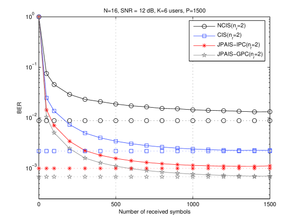
Figure 6: BER performance versus number of symbols. The curves for the adaptive schemes are in solid lines, whereas those of the optimal MMSE schemes are in dotted lines. Parameters: $\lambda_{T}=\lambda_{k}=0.025$ (for MMSE schemes), $\alpha=0.998$ (for adaptive schemes).

The second experiment depicted in Fig. 6 shows the BER performance of the proposed adaptive algorithms (JPAIS) against the existing NCIS and CIS schemes with $n_{r}=2$ relays. All techniques employ RLS algorithms for the estimation of the coefficients of the channel, the receive filters and the power allocation for each user (JPAIS only). The complexity of the proposed algorithms is quadratic with the filter length of the receivers and the number of relays $n_{r}$, whereas the optimal MMSE schemes require cubic complexity. From the results, we can verify that the proposed adaptive joint estimation algorithms converge to approximately the same level of the MMSE schemes, which have full knowledge of the channel and the noise variance. Again, the proposed JPAIS-GPC is superior to the JPAIS-IPC but requires higher complexity and joint demodulation of signals, whereas the JPAIS-IPC lends itself to a distributed implementation.

Figure 7: BER performance versus $f_{d}T$. The parameters of the adaptive algorithms are optimized for each $f_{d}T$.

The next experiment considers the average BER performance against the normalized fading rate $f_{d}T$ (cycles/symbol), as depicted in Fig. 7. The idea is to illustrate a situation where the channel changes within a packet and the system transmits the power allocation vectors computed by the proposed JPAIS algorithms via a feedback channel. In this scenario, the JPAIS algorithms compute the parameters of the receiver and the power allocation vector, which is transmitted only once to the mobile users. This leads to a situation in which the power allocation becomes outdated. The results show that the gains of the proposed JPAIS algorithms decrease gradually as the $f_{d}T$ is increased to the BER level of the existing CIS algorithms for both $n_{r}=2$ and $n_{r}=4$ relays, indicating that the power allocation is no longer able to provide performance advantages. This problem requires the deployment of a frequent update of the power allocation via feedback channels. Therefore, the proposed JPAIS algorithms are suitable for scenarios with $f_{d}T<10^{-3}$ for which there are performance gains.

The algorithms are now assessed in terms of the mutual information between the $k$-th user and the base station as suggested in [11] and the normalized throughput (NT) defined as $NT=R(1-BER)^{P~{}log_{2}M}$ in bits/time slot, where $R$ is the normalized rate, $M$ is the number of points in the constellation and $P$ is the packet size in symbols. Since the protocols operate at full rate in a synchronous system and QPSK modulation is used the parameter used are $R=1$ and $M=4$. The results are shown in Fig. 8 and indicate that the JPAIS algorithms can obtain gains in terms of the mutual information and the NT for a sufficiently high SNR level. When the SNR is low the use of more phases of transmission (or time slots) can degrade the NT and the mutual information of the system. The use of the proposed JPAIS algorithms with multihop transmission is not recommended in these situations. However, as the SNR is increased the proposed JPAIS algorithms obtain the best results with $n_{r}=1,2$. The JPAIS-GPC algorithm achieves the best NT results followed by the JPAIS-IPC and the CIS techniques.

Figure 8: (a) Mutual information (bits/Hz) versus SNR (dB) and (b) the normalized throughput (bits/time slot) versus SNR (dB).

The last experiment, shown in Fig. 9, illustrates the averaged BER performance versus the percentage of errors in the feedback channel for an uplink scenario. Specifically, the feedback packet structure is employed and each coefficient is quantized with $4$ bits. Each feedback packet is constructed with a sequence of binary data ($0$s and $1$s) and is transmitted over a binary symmetric channel (BSC) with an associated probability of error $P_{e}$. We then evaluate the BER of the proposed JPAIS and the existing algorithms against several values of the $P_{e}$. The results show that the proposed JPAIS algorithms obtain significant gains over the existing CIS algorithm for values of $P_{e}<0.1\%$. As we increase the rate of feedback errors, the performance of the proposed JPAIS algorithms becomes worse than the CIS algorithms and are no longer suitable. This suggests the use of error-control coding techniques to keep the level of errors in the feedback channel below a certain value.

Figure 9: BER performance versus $f_{d}T$. The parameters of the adaptive algorithms are optimized for each $f_{d}T$.

VIII Concluding remarks and extensions

We have presented in this work joint iterative power allocation and interference mitigation techniques for DS-CDMA networks which employ multiple hops and the AF cooperation strategy. A joint constrained optimization framework and algorithms that consider the allocation of power levels across the relays subject to global and individual power constraints and the design of linear receivers for interference suppression have been proposed. A study of the proposed optimization problems has been carried out and has shown that the convexity of the problem can be enforced via an appropriate choice of the global and individual power constraints. A study of the requirements of the proposed and existing algorithms in terms of computational complexity and feedback channels has also been conducted. The results of simulations have shown that the proposed JPAIS techniques obtain significant gains in performance and capacity over existing non-cooperative and cooperative schemes. The proposed JPAIS algorithms can be employed in a variety of wireless communications systems with relays including multiple-antenna, orthogonal-frequency-division-multiplexing (OFDM) and ultra-wide band (UWB) systems. Prior work on asymptotic results has been reported in [22] and [23] for $2$-phase systems without power allocation. A possible extension would be to use the power allocation strategy of this work and investigate the asymptotic gains.

References

• [1] A. Sendonaris, E. Erkip, and B. Aazhang, โ€User cooperation diversity - Parts I and II,โ€ IEEE Trans. Commun., vol. 51, no. 11, pp. 1927-1948, November 2003.
• [2] J. N. Laneman and G. W. Wornell, โ€Distributed space-time-coded protocols for exploiting cooperative diversity in wireless networks,โ€ IEEE Trans. Inf. Theory, vol. 49, no. 10, pp. 2415-2425, Oct. 2003.
• [3] J. N. Laneman and G. W. Wornell, โ€Cooperative diversity in wireless networks: Efficient protocols and outage behaviour,โ€ IEEE Trans. Inf. Theory, vol. 50, no. 12, pp. 3062-3080, Dec. 2004.
• [4] W. J. Huang, Y. W. Hong and C. C. J. Kuo, โ€œDecode-and-forward cooperative relay with multi-user detection in uplink CDMA networks,โ€ in Proc. IEEE Global Telecommunications Conference, November 2007, pp. 4397-4401.
• [5] G. Kramer, M. Gastpar and P. Gupta, โ€œCooperative strategies and capacity theorems for relay networks,โ€ IEEE Trans. Inf. Theory, vol. 51, no. 9, pp. 3037-3063, September 2005.
• [6] J. Luo, R. S. Blum, L. J. Cimini, L. J Greenstein and A. M. Haimovich, โ€œDecode-and-Forward Cooperative Diversity with Power Allocation in Wireless Networksโ€, IEEE Transactions on Wireless Communications, vol. 6, no. 3, pp. 793 - 799, March 2007.
• [7] L. Long and E. Hossain, โ€œCross-layer optimization frameworks for multihop wireless networks using cooperative diversityโ€œ, IEEE Transactions on Wireless Communications, vol. 7, no. 7, pp. 2592-2602, July 2008.
• [8] P. Clarke and R. C. de Lamare, โ€œJoint Transmit Diversity Optimization and Relay Selection for Multi-relay Cooperative MIMO Systems Using Discrete Stochastic Algorithmsโ€, IEEE Communications Letters, vol. 15, no. 10, 2011, pp.1035-1037.
• [9] P. Clarke ad R. C. de Lamare, โ€Transmit Diversity and Relay Selection Algorithms for Multi-relay Cooperative MIMO Systemsโ€, IEEE Transactions on Vehicular Technology, vol. 61 , no. 3, March 2012, Page(s): 1084 - 1098.
• [10] L. Venturino, X. Wang and M. Lops, โ€œMultiuser detection for cooperative networks and performance analysis,โ€ IEEE Trans. Sig. Proc., vol. 54, no. 9, September 2006.
• [11] K. Vardhe, D. Reynolds and M. C. Valenti, โ€œThe performance of multi-user cooperative diversity in an asynchronous CDMA uplinkโ€, IEEE Transactions on Wireless Communications, vol. 7, no. 5, Part 2, May 2008, pp. 1930 - 1940.
• [12] W. Fang, L. L. Yang, and L. Hanzo, โ€œPerformance of DS-CDMA downlink using transmitter preprocessing and relay diversity over Nakagami-m fading channelsโ€, IEEE Transactions on Wireless Communications, vol. 8, no. 2, pp. 678-682, 2009.
• [13] L. L. Yang, W. Fang, โ€œPerformance of Distributed-Antenna DS-CDMA Systems Over Composite Lognormal Shadowing and Nakagami-m-Fading Channelsโ€, IEEE Transactions on Vehicular Technology, vol. 58, no. 6, pp. 2872-2883, 2009.
• [14] M. R. Souryal, B. R. Vojcic and R. Pickholtz, โ€œAdaptive modulation in ad hoc DS/CDMA packet radio networksโ€, IEEE Transactions on Communications, vol. 54, no. 4, April 2006 pp. 714 - 725.
• [15] C. Comaniciu, and H. V. Poor, โ€œOn the capacity of mobile ad hoc networks with delay constraintsโ€ IEEE Transactions on Wireless Communications, vol. 5, no. 8, August 2006, pp.2061 - 2071.
• [16] M. Levorato, S. Tomasin, M. Zorzi, โ€œCooperative spatial multiplexing for ad hoc networks with hybrid ARQ: system design and performance analysisโ€, IEEE Transactions on Communications, vol. 56, no. 9, September 2008. pp. 1545 - 1555.
• [17] C.Fischione, K. H. Johansson, A. Sangiovanni-Vincentelli, B. Zurita Ares, โ€œMinimum Energy coding in CDMA Wireless Sensor Networks,โ€ IEEE Transactions on Wireless Communications, vol. 8, no. 2, Feb. 2009, pp. 985 - 994.
• [18] T. Kastrinogiannis, V. Karyotis, S. Papavassiliou, โ€œAn Opportunistic Combined Power and Rate Allocation Approach in CDMA Ad Hoc Networksโ€, 2008 IEEE Sarnoff Symposium, 28-30 April 2008.
• [19] G. Jakllari, S. V. Krishnamurthy , M. Faloutsos, and P. V. Krishnamurthy, โ€œOn Broadcasting with Cooperative Diversity in Multi-hop Wireless Networksโ€, IEEE Journal on Selected Areas in Communications, vol. 25, no. 2, February 2007.
• [20] C.-H. Liu, โ€œEnergy-Optimized Low-Complexity Control of Power and Rate in Clustered CDMA Sensor Networks with Multirate Constraintsโ€, Proc. IEEE 66th Vehicular Technology Conference, 30 Sept. - 3 Oct. 2007, pp. 331 - 335.
• [21] M. Chen, C. Oh and A. Yener,โ€œEfficient Scheduling for Delay Constrained CDMA Wireless Sensor Networksโ€, Proc. IEEE 64th Vehicular Technology Conference, VTC-2006 Fall. 2006, 25-28 September 2006.
• [22] D. Gregoratti and X. Mestre, โ€œRandom DS/CDMA for the Amplify and Forward Relay Channelโ€, IEEE Transactions on Wireless Communications, vol. 8, no. 2, February 2009.
• [23] K. Zarifi, S. Affes and A. Ghrayeb, โ€œLarge-System-Based Performance Analysis and Design of Multiuser Cooperative Networksโ€, IEEE Transactions on Signal Processing, vol. 57, no. 4, April 2009.
• [24] S. Verdu, Multiuser Detection, Cambridge, 1998.
• [25] R. C. de Lamare and R. Sampaio-Neto, โ€œAdaptive Interference Suppression for DS-CDMA Systems based on Interpolated FIR Filters with Adaptive Interpolators in Multipath Channelsโ€, IEEE Trans. Vehicular Technology, Vol. 56, no. 6, September 2007, 2457 - 2474.
• [26] R. C. de Lamare and R. Sampaio-Neto, โ€œMinimum Mean Squared Error Iterative Successive Parallel Arbitrated Decision Feedback Detectors for DS-CDMA Systems,โ€ IEEE Transactions on Communications, vol. 56, no. 5, May 2008, pp. 778 - 789.
• [27] R.C. de Lamare, R. Sampaio-Neto, A. Hjorungnes, โ€œJoint iterative interference cancellation and parameter estimation for cdma systemsโ€, IEEE Communications Letters, vol. 11, no. 12, December 2007, pp. 916 - 918.
• [28] Y. Cai and R. C. de Lamare, โ€Adaptive Space-Time Decision Feedback Detectors with Multiple Feedback Cancellationโ€, IEEE Transactions on Vehicular Technology, vol. 58, no. 8, October 2009, pp. 4129 - 4140.
• [29] R. C. de Lamare, โ€œJoint Power Allocation and Interference Suppression Techniques for Cooperative CDMA Systems โ€, Proc. IEEE Vehicular Technology Conference, VTC-2009 Spring, Barcelona, 2009.
• [30] R. C. de Lamare and S. Li, โ€œJoint Iterative Power Allocation and Interference Suppression Algorithms for Cooperative DS-CDMA Networksโ€, Proc. IEEE Vehicular Technology Conference, VTC-2010 Spring, Taipei, 2010.
• [31] I. Csiszar and G. Tusnisdy, โ€œInformation geometry and alternating minimization procedures,โ€ Statistics and Decisions, Supplement Issue, no. l, pp. 205-237, 1984.
• [32] U. Niesen, D. Shah, and G. W. Wornell, โ€œAdaptive Alternating Minimization Algorithmsโ€, IEEE Trans. Inform. Theory, vol. 55, no. 3, pp. 1423-1429, Mar. 2009.
• [33] R. C. de Lamare and R. Sampaio-Neto, โ€œReduced-Rank Adaptive Filtering Based on Joint Iterative Optimization of Adaptive Filtersโ€, IEEE Signal Processing Letters, Vol. 14, no. 12, December 2007.
• [34] R. C. de Lamare and R. Sampaio-Neto, โ€œReduced-Rank Space-Time Adaptive Interference Suppression With Joint Iterative Least Squares Algorithms for Spread-Spectrum Systems,โ€ IEEE Transactions on Vehicular Technology, vol.59, no.3, March 2010, pp.1217-1228.
• [35] M. L. Honig and J. S. Goldstein, โ€œAdaptive reduced-rank interference suppression based on the multistage Wiener filter,โ€ IEEE Trans. Commun., vol. 50, pp. 986-994, June 2002.
• [36] H. Qian and S. N Batalama, โ€œData record-based criteria for the selection of an auxiliary vector estimator of the MMSE/MVDR filterยดยด IEEE Trans. on Commun., vol. 51, No. 10, October 2003, pp. 1700-1708.
• [37] R. C. de Lamare and R. Sampaio-Neto, โ€œAdaptive Reduced-Rank Processing Based on Joint and Iterative Interpolation, Decimation, and Filtering,โ€ IEEE Transactions on Signal Processing, vol. 57, no. 7, July 2009, pp. 2503 - 2514.
• [38] R.C. de Lamare, R. Sampaio-Neto and M. Haardt, โ€Blind Adaptive Constrained Constant-Modulus Reduced-Rank Interference Suppression Algorithms Based on Interpolation and Switched Decimation,โ€ IEEE Trans. on Signal Processing, vol.59, no.2, pp.681-695, Feb. 2011.
• [39] S. Haykin, Adaptive Filter Theory, 4th ed. Englewood Cliffs, NJ: Prentice- Hall, 2002.
• [40] G. H. Golub and C. F. van Loan, Matrix Computations, 3rd ed., The Johns Hopkins University Press, Baltimore, Md, 1996.
• [41] D. Luenberger, Linear and Nonlinear Programming, 2nd Ed. Addison-Wesley, Inc., Reading, Massachusetts 1984.
• [42] A. Gersho and R. M. Gray, Vector Quantization and Signal Compression, Kluwer Academic Press/Springer, 1992.
• [43] R. C. de Lamare and A. Alcaim, โ€Strategies to improve the performance of very low bit rate speech coders and application to a 1.2 kb/s codecโ€ IEE Proceedings- Vision, image and signal processing, vol. 152, no. 1, February, 2005.
• [44] T. S. Rappaport, Wireless Communications, Prentice-Hall, Englewood Cliffs, NJ, 1996.