Set-Membership Adaptive Algorithms based on Time-Varying Error Bounds for Interference Suppression

Abstract

This work presents set-membership adaptive algorithms based on time-varying error bounds for CDMA interference suppression. We introduce a modified family of set-membership adaptive algorithms for parameter estimation with time-varying error bounds. The algorithms considered include modified versions of the set-membership normalized least mean squares (SM-NLMS), the affine projection (SM-AP) and the bounding ellipsoidal adaptive constrained (BEACON) recursive least-squares technique. The important issue of error bound specification is addressed in a new framework that takes into account parameter estimation dependency, multi-access and inter-symbol interference for DS-CDMA communications. An algorithm for tracking and estimating the interference power is proposed and analyzed. This algorithm is then incorporated into the proposed time-varying error bound mechanisms. Computer simulations show that the proposed algorithms are capable of outperforming previously reported techniques with a significantly lower number of parameter updates and a reduced risk of overbounding or underbounding.

I Introduction

Set-membership filtering (SMF) [2, 3, 4, 5] represents a class of recursive estimation algorithms that, on the basis of a pre-determined error bound, seeks a set of parameters that yield bounded filter output errors. These algorithms have been used in a variety of applications such as adaptive equalization [6] and multi-access interference suppression [7, 8]. The SMF algorithms are able to combat conflicting requirements such as fast convergence and low misadjustment by introducing a modification on the objective function. In addition, these algorithms exhibit reduced complexity due to data-selective updates, which involve two steps: a) information evaluation and b) update of parameter estimates. If the filter update does not occur frequently and the information evaluation does not involve much computational complexity, the overall complexity can be significantly reduced.

The adaptive SMF algorithms usually achieve good convergence and tracking performance due to an adaptive step size for each update, and reduced complexity resulting from data selective updating. However, the performance of SMF techniques depends on the error-bound specification, which is very difficult to obtain in practice due to the lack of knowledge of the environment and its dynamics. In wireless networks characterized by non-stationary environments, where users often enter and exit the system, it is very difficult to choose an error bound and the risk of overbounding (when the error bound is larger than the actual one) and underbounding (when the error bound is smaller than the actual one) is significantly increased, leading to performance degradation. In addition, when the measured noise in the system is time-varying and the multiple access interference (MAI) and the intersymbol interference (ISI) encountered by a receiver in a communication system are highly dynamic, the selection of an error-bound is further complicated. This is especially relevant for low-complexity estimation problems encountered in applications such as mobile terminals and wireless sensor networks [9], where the sensors have limited signal processing capabilities and power consumption is of central importance. These problems suggest the deployment of mechanisms to automatically adjust the error bound in order to guarantee good performance and a small update rate (UR). It should also be remarked that most of prior work on adaptive algorithms for interference suppression [19] is restricted to systems with short codes. However, the proposed adaptive techniques are also applicable to systems with long codes provided some modifications are carried out. For downlink scenarios, the designer can resort to chip equalization [25] followed by a despreader. For an uplink solution, channel estimation algorithms for aperiodic sequences [26, 27] are required and the sample average approach for estimating the covariance matrix ${\bf R}=E[{\bf r}(i){\bf r}^{H}(i)]$ of the observed data ${\bf r}(i)$ has to be replaced by $\hat{\bf R}={\bf P}{\bf P}^{H}+\sigma^{2}{\bf I}$, which is constructed with a matrix ${\bf P}$ containing the effective signature sequence of users and the variance $\sigma^{2}$ of the receiver’s noise [28].

Previous works on time-varying error bounds include the tuning of noise bounds in [10, 11], the approach in [14] which assumes that the ”true” error bound is constant, and the parameter-dependent error bound recently proposed in [12, 13] with frequency-domain estimation algorithms. The techniques so far reported do not introduce any mechanism for tracking the MAI and the ISI and incorporating their power estimates in the error bound. In addition, the existing approaches with time-varying bounds have not been considered for more sophisticated adaptive filtering algorithms such as the affine projection (AP) and the least-squares (LS) based techniques.

In this work, we propose and analyze a low-complexity framework for tracking parameter evolution and MAI and ISI power levels, that relies on simple channel and interference estimation techniques, and encompasses a family of set-membership algorithms [3, 4, 7, 15] with time-varying error bounds. Specifically, we present modified versions of the set-membership normalized least mean squares (SM-NLMS) [3], the affine projection [4] (SM-AP) and the bounding ellipsoidal adaptive constrained (BEACON) [7, 15] recursive least-squares (RLS) algorithm for parameter estimation. Then, we incorporate the proposed mechanisms of interference estimation and tracking into the time-varying error bounds. In order to evaluate the proposed algorithms, we consider a DS-CDMA interference suppression application and adaptive linear multiuser receivers in situations of practical interest.

This work is organized as follows. Section II briefly describes the DS-CDMA system model and linear receivers. Section III reviews the SMF concept with time-varying error bounds and is devoted to the derivation of adaptive algorithms. Section IV presents the framework for time-varying error bounds and the proposed algorithms for channel, interference estimation and tracking. Section V is dedicated to the analysis of the algorithms for channel, amplitude, interference estimation and their tracking. Section VI shows and discusses the simulations results, while Section VII gives the conclusions.

II DS-CDMA System Model and Linear Receivers

Let us consider the downlink of a symbol synchronous DS-CDMA system with $K$ users, $N$ chips per symbol and $L_{p}$ propagation paths [19]. We assume that the delay is a multiple of the chip rate, the channel is constant during each symbol interval and the spreading codes are repeated from symbol to symbol. The received signal $r(t)$ after filtering by a chip-pulse matched filter and sampled at chip rate yields the $M$-dimensional received vector

$$\begin{split}{\bf r}[i]&=\sum_{k=1}^{K}A_{k}[i]{b}_{k}[i]{\bf C}_{k}{\bf h}[i]+{\boldsymbol{\eta}}[i]+{\bf n}[i],\end{split}$$ (1)

where $M=N+L_{p}-1$, ${\bf n}[i]=[n_{1}[i]~{}\ldots~{}n_{M}[i]]^{T}$ is the complex Gaussian noise vector with zero mean and covariance matrix $E[{\bf n}[i]{\bf n}^{H}[i]]=\sigma^{2}{\bf I}$, where $(\cdot)^{T}$ and $(\cdot)^{H}$ denote transpose and Hermitian transpose, respectively. The quantity $E[\cdot]$ stands for expected value, the user $k$ symbol is $b_{k}[i]$ and is assumed to be drawn from a general constellation. The amplitude of user $k$ is $A_{k}[i]$ and ${\boldsymbol{\eta}}[i]$ is the intersymbol interference (ISI) for user $k$. The $M\times L_{p}$ convolution matrix ${\bf C}_{k}$ that contains one-chip shifted versions of the signature sequence for user $k$ expressed by ${\bf s}_{k}=[a_{k}(1)\ldots a_{k}(N)]^{T}$ and the $L_{p}\times 1$ vector ${\bf h}[i]$ with the multipath components are described by:

$${\bf C}_{k}=\left[\begin{array}[]{c c c }a_{k}(1)&&{\bf 0}\\ \vdots&\ddots&a_{k}(1)\\ a_{k}(N)&&\vdots\\ {\bf 0}&\ddots&a_{k}(N)\\ \end{array}\right],{\bf h}[i]=\left[\begin{array}[]{c}{h}_{0}[i]\\ \vdots\\ {h}_{L_{p}-1}[i]\\ \end{array}\right].$$ (2)

In this model, the ISI span and contribution ${\boldsymbol{\eta}}_{k}[i]$ are functions of the processing gain $N$ and $L_{p}$. If $1<L_{p}\leq N$ then $3$ symbols would interfere in total, the current one, the previous and the successive symbols. In the case of $N<L_{p}\leq 2N$ then $5$ symbols would interfere, the current one, the $2$ previous and the $2$ successive ones. In most practical CDMA systems, we have that $1<L_{p}\leq N$ and then only $3$ symbols are usually affected. The reader is referred to UMTS channel models [23], which reveal that the channel usually affects at most $3$ symbols (it typically spans a few chips).

The multiuser linear receiver design corresponds to determining an FIR filter ${\bf w}_{k}[i]=\big{[}w_{0}[i]~{}w_{1}[i]~{}\ldots~{}w_{M-1}\big{]}^{T}$ with $M$ coefficients that provides an estimate of the desired symbol as given by

$$\hat{b}_{k}[i]=\textrm{sgn}\Big{(}\Re\Big{[}{\bf w}_{k}^{H}[i]{\bf r}[i]\Big{]}\Big{)}=\textrm{sgn}\Big{(}\Re\Big{[}{z}_{k}[i]\Big{]}\Big{)},$$ (3)

where the quantity $\Re(\cdot)$ selects the real part and $\textrm{sgn}(\cdot)$ is the signum function. The quantity $z_{k}[i]={\bf w}_{k}^{H}[i]{\bf r}[i]$ is the output of the receiver parameter vector ${\bf w}_{k}$ for user $k$, which is optimized according to a chosen criterion.

III Set-Membership Adaptive Algorithms with Time-Varying Error Bounds and Problem Statement

In this section, we describe a framework that encompasses modified set-membership (SM) adaptive algorithms with time-varying error bounds for communications applications. In an SM filtering [3] framework, the parameter vector ${\bf w}_{k}[i]$ for user $k$ in a multi-access system is designed to achieve a specified bound on the magnitude of the estimation error $e_{k}[i]=b_{k}[i]-{\bf w}_{k}^{H}[i]{\bf r}[i]$. As a result of this constraint, the SM adaptive algorithm will only perform filter updates for certain data. Let $\Theta_{k}[i]$ represent the set containing all ${\bf w}_{k}[i]$ that yields an estimation error upper bounded in magnitude by a time-varying error bound $\gamma_{k}[i]$. Thus, we can write

$$\Theta_{k}[i]=\bigcap_{{(b_{k}[i],~{}{\bf r}[i])\in{\boldsymbol{S}}_{k}}}\{{\bf w}_{k}\in{\mathcal{C}}^{M}:\mid e_{k}[i]\mid\leq\gamma_{k}[i]\},$$ (4)

where ${\bf r}[i]$ is the observation vector, ${\boldsymbol{S}}_{k}$ is the set of all possible data pairs $(b_{k}[i],~{}{\bf r}[i])$ and the set $\Theta_{k}[i]$ is referred to as the feasibility set for user $k$, and any point in it is a valid estimate ${z}_{k}[i]={\bf w}_{k}^{H}[i]{\bf r}[i]$. Since it is not practical to predict all data pairs, adaptive methods work with the membership sets $\psi_{k,i}=\bigcap_{m=1}^{i}{\mathcal{H}}_{k,m}$ provided by the observations, where ${\mathcal{H}}_{k,m}=\{{\bf w}_{k}\in{\mathcal{C}}^{M}:|b_{k}[m]-z_{k}[m]|\leq\gamma_{k}[m]\}$ is the constraint set. It can be seen that the feasibility set $\Theta_{k}[i]$ is a subset of the exact membership set at any given time instant. The feasibility set $\Theta_{k}[i]$ is also the limiting set of the exact membership set, i.e., the two sets will be equal if the training signal traverses all signal pairs belonging to ${\boldsymbol{S}}_{k}$. The idea of the SM algorithms is to adaptively find an estimate that belongs to the feasibility set $\Theta_{k}[i]$. One alternative is to apply one of the many OBE algorithms such as the bounding ellipsoidal adaptive constrained (BEACON) [15, 7] recursive least-squares (RLS) algorithm, which tries to approximate the exact membership set with ellipsoids. Another way is to compute a point estimate through projections using, for example, the information provided by the constraint set ${\mathcal{H}}_{k,i}$, as done by the set-membership NLMS (SM-NLMS) and the affine projection [4] (SM-AP) algorithms. In order to devise an effective SM algorithm, the error bound $\gamma_{k}[i]$ must be appropriately chosen. Due to time-varying nature of many practical environments, this error bound should also be adaptive and adjustable to certain characteristics of the environment for the SM estimation technique. The natural question that arises is: how to design an efficient and effective mechanism to adjust $\gamma_{k}[i]$? In what follows, we will present a modified family of SM adaptive algorithms that rely on general time-varying error bounds. Specifically, we will consider the SM-NLMS [3], SM-AP [4] and BEACON [15, 7] algorithms and we will modify them such that they will operate with general time-varying error bounds.

III-A SM-NLMS Algorithm with Time-Varying Bounds

In order to derive an SM-NLMS adaptive algorithm with time-varying bounds using point estimates, we consider the following optimization problem

$$\begin{split}{\textrm{minimize}}&~{}||{\bf w}_{k}[i+1]-{\bf w}_{k}[i]||^{2}\\ {\textrm{subject to}}&~{}(b_{k}[i]-{\bf w}_{k}^{H}[i+1]{\bf r}[i])={g}_{k}[i]\end{split}$$ (5)

In order to solve the above constrained optimization problem, we resort to the method of Lagrange multipliers [2, 24], which yields the unconstrained cost function

$$\begin{split}{\mathcal{L}}&=||{\bf w}_{k}[i+1]-{\bf w}_{k}[i]||^{2}+2\Re\Big{[}{\bf\lambda}^{*}(b_{k}[i]-{\bf w}_{k}^{H}[i+1]{\bf r}[i]-g_{k}[i])\Big{]},\end{split}$$ (6)

where $*$ denotes complex conjugate, ${\bf\lambda}$ is a Lagrange multiplier and $g_{k}[i]$ is the time-varying set-membership constraint for user $k$. Taking the gradient terms of (6) with respect to ${\bf w}_{k}[i+1]$ and ${\bf\lambda}*$, and setting them to zero, leads us to a system of equations. Solving these equations yields:

$$e_{k}[i]=b_{k}[i]-{\bf w}_{k}^{H}[i]{\bf r}[i],$$ (7)

$${\bf w}_{k}[i+1]={\bf w}_{k}[i]+({\bf r}^{H}[i]{\bf r}[i])^{-1}(e_{k}[i]-g_{k}[i])^{*}{\bf r}[i],$$ (8)

where $e_{k}[i]$ is the error for user $k$. By choosing $g_{k}[i]$ such that $e_{k}[i]$ lies on the closest boundary of $\Theta_{k}[i]$ and considering a time-varying error bound $\gamma_{k}[i]$, i.e., $g_{k}[i]=\gamma_{k}[i]sgn(e_{k}[i])$ [3], we obtain the following data dependent update rule and step size

$${\bf w}_{k}[i+1]={\bf w}_{k}[i]+\mu_{w}[i]e_{k}^{*}[i]{\bf r}[i],$$ (9)

$$\mu_{w}[i]=\left\{\begin{array}[]{ll}\frac{1}{{\bf r}^{H}[i]{\bf r}[i]}(1-\gamma_{k}[i]/|e_{k}^{*}[i]|)&\textrm{if $|e_{k}^{*}[i]|>\gamma_{k}[i]$,}\\ 0&\textrm{otherwise.}\\ \end{array}\right.$$ (10)

III-B SM-AP Algorithm with Time-Varying Bounds

In order to describe a modified SM-AP algorithm with time-varying bounds, let us first define the observation matrix ${\bf Y}[i]=[{\bf r}[i]~{}\ldots~{}{\bf r}[i-P+1]]$, the desired output vector ${\bf b}_{k}[i]=[b_{k}[i]~{}\ldots~{}b_{k}[i-P+1]]^{T}$ that comprises $P$ outputs and the error vector

$${\bf e}_{k}[i]=\left[\begin{array}[]{c}{b^{*}_{k}[i]-{\bf r}^{H}[i]{\bf w}_{k}[i]}\\ \vdots\\ {b^{*}_{k}[i]-{\bf r}^{H}[i-P+1]{\bf w}_{k}[i]}\\ \end{array}\right]={\bf b}^{*}_{k}[i]-{\bf Y}^{H}[i]{\bf w}_{k}[i].$$ (11)

The SM-AP adaptive algorithm with time-varying bounds can be derived from the optimization problem

$$\begin{split}{\textrm{minimize}}&~{}||{\bf w}_{k}[i+1]-{\bf w}_{k}[i]||^{2}\\ {\textrm{subject to}}&~{}({\bf b}_{k}[i]-{\bf Y}^{H}[i]{\bf w}_{k}[i+1])={\bf g}_{k}[i].\end{split}$$ (12)

In order to solve the above problem, we employ the method of Lagrange multipliers and consider the unconstrained cost function

$$\begin{split}{\mathcal{L}}&=||{\bf w}_{k}[i+1]-{\bf w}_{k}[i]||^{2}+2\Re\Big{[}({\bf b}_{k}[i]-{\bf Y}^{H}[i]{\bf w}_{k}[i+1]-{\bf g}_{k}[i])^{H}\boldsymbol{\lambda}\Big{]},\end{split}$$ (13)

where $\boldsymbol{\lambda}$ is the vector with Lagrange multipliers and ${\bf g}_{k}[i]$ is a constraint vector. By calculating the gradient terms of (13) with respect to ${\bf w}_{k}[i+1]$ and ${\boldsymbol{\lambda}}$, setting them to zero and solving the resulting equations we arrive at the following algorithm:

$${\bf t}_{k}[i]=({\bf Y}^{H}[i]{\bf Y}[i]+\delta{\bf I})^{-1}({\bf e}_{k}[i]-{\bf g}[i]),$$ (14)

$${\bf w}_{k}[i+1]={\bf w}_{k}[i]+{\bf Y}[i]{\bf t}_{k}[i],$$ (15)

where $\delta$ is a small constant inserted in addition to the term ${\bf Y}^{H}[i]{\bf Y}[i]$ for improving robustness. If we select ${\bf e}_{k}[i]-{\bf g}_{k}[i]=(e_{k}[i]-\gamma sgn(e_{k}[i])){\bf u}=(1-\gamma_{k}[i]/|e_{k}[i]|)e_{k}[i]{\bf u}$, where the a posteriori errors $e_{k}[i-j]$ are kept constant for $j=1,~{}\ldots,P-1$ and ${\bf u}=[1~{}0~{}\ldots~{}0]^{T}$, we obtain the following recursion for the update of ${\bf t}_{k}[i]$:

$${\bf t}_{k}[i]=({\bf Y}^{H}[i]{\bf Y}[i]+\delta{\bf I})^{-1}(1-\gamma/|e_{k}[i]|)e_{k}[i]{\bf u}.$$ (16)

Substituting (16) into (15) and using the bound constraint, we obtain the following SM-AP algorithm:

$${\bf w}_{k}[i+1]={\bf w}_{k}[i]+\mu_{w}[i]{\bf Y}[i]({\bf Y}^{H}[i]{\bf Y}[i]+\delta{\bf I})^{-1}e_{k}[i]{\bf u},$$ (17)

$$\mu_{w}[i]=\left\{\begin{array}[]{ll}(1-\gamma_{k}[i]/|e_{k}[i]|)&\textrm{if $|e_{k}[i]|>\gamma_{k}[i]$,}\\ 0&\textrm{otherwise.}\\ \end{array}\right.$$ (18)

The SM-AP algorithm described here has computational complexity of $UR\times{\mathcal{O}}(PM+2K_{inv}P^{2})$, where $K_{inv}$ is a factor required to invert a $P\times P$ matrix [2] and $UR$ is the update rate. Note that the SM-AP is a generalized case of the SM-NLMS where $P$ data vectors are used to increase the convergence speed.

III-C BEACON Adaptive Algorithm with Time-Varying Bounds

Here, we propose a modification for a computationally efficient version of an optimal bounding ellipsoidal (OBE) algorithm called the Bounding Ellipsoidal Adaptive Constrained Least-Squares (BEACON) algorithm [7], which is closely related to a constrained least-squares optimization problem. The proposed technique amounts to deriving the BEACON algorithm equipped with time-varying bounds. Unlike the other previously reported low-complexity algorithms [3, 4] and the modified SM-NLMS and SM-AP techniques described in the previous subsections, the modified BEACON recursion has the potential to achieve a very fast convergence performance, which is relatively independent from the eigenvalue spread of the data covariance matrix as compared to the stochastic gradient algorithms [2].

The proposed BEACON algorithm with a time-varying bound can be derived from the following optimization problem [7]

$$\begin{split}{\textrm{minimize}}&~{}\sum_{l=1}^{i-1}\lambda^{i-l}[l]|b_{k}[l]-{\bf w}_{k}^{H}[i]{\bf r}[l]|^{2}\\ {\textrm{subject to}}&~{}|{\bf b}_{k}[i]-{\bf w}_{k}[i]^{H}{\bf r}[i]|^{2}=\gamma_{k}^{2}[i].\end{split}$$ (19)

The constrained problem above can be recast as an unconstrained one and be solved via an unconstrained least-squares cost function using the method of Lagrange multipliers given by

$$\begin{split}{\mathcal{L}}&=\sum_{l=1}^{i-1}\lambda_{k}[l]^{i-l}|b_{k}[l]-{\bf w}^{H}_{k}[i]{\bf r}[l]|^{2}+\lambda_{k}[i](|b_{k}[i]-{\bf w}^{H}_{k}[i]{\bf r}[i]|^{2}-\gamma_{k}^{2}[i]),\end{split}$$ (20)

where $\lambda_{k}[l]$ plays the role of Lagrange multiplier and forgetting factor at the same time for user $k$. The solution to the above optimization problem is obtained by taking the gradient terms with respect to ${\bf w}_{k}[i]$ and making them equal to zero. After some mathematical manipulations we have

$${\bf w}_{k}[i]={\bf w}_{k}[i-1]+\lambda_{k}[i]{\bf P}_{k}[i]{\bf r}[i](b_{k}[i]-{\bf w}^{H}_{k}[i]{\bf r}[i])^{*}.$$ (21)

By using the constraint $b_{k}[i]-{\bf w}^{H}_{k}[i]{\bf r}[i]=(\xi_{k}[i]/|\xi_{k}[i]|)\gamma_{k}[i]=\xi_{k}[i]-(\lambda_{k}[i]{\bf G}_{k}[i](\xi_{k}[i]/|\xi_{k}[i]|)\gamma_{k}[i])$, and the matrix inversion lemma [2], we can arrive at the BEACON algorithm with time-varying bounds described by

$${\bf P}_{k}[i]={\bf P}_{k}[i-1]-\frac{\lambda_{k}[i]{\bf P}_{k}[i-1]{\bf r}[i]{\bf r}^{H}[i]{\bf P}_{k}[i-1]}{1+\lambda_{k}[i]t_{k}[i]},$$ (22)

$${\bf w}_{k}[i]={\bf w}_{k}[i-1]+\lambda_{k}[i]{\bf P}_{k}[i]{\bf r}[i]\xi^{*}_{k}[i],$$ (23)

where the prediction error is $\xi_{k}[i]=b_{k}[i]-{\bf w}^{H}_{k}[i-1]{\bf r}[i]$, $t_{k}[i]={\bf r}^{H}[i]{\bf P}_{k}[i-1]{\bf r}[i]$, and $\lambda_{k}[i]\geq 0$. In order to compute the optimal value for $\lambda_{k}[i]$, the algorithm considers the following cost function [7]:

$${\mathcal{C}}_{\lambda_{k}[i]}=\lambda_{k}[i]\Bigg{[}\frac{\xi_{k}[i]}{\gamma^{2}_{k}[i]}\Bigg{(}\frac{1}{1+\lambda_{k}[i]t_{k}[i]}\Bigg{)}-1\Bigg{]}.$$ (24)

The minimization of the cost function in (24) leads to the innovation check of the proposed BEACON algorithm:

$$\lambda_{k}[i]=\left\{\begin{array}[]{ll}\frac{1}{t_{k}[i]}\Bigg{(}\frac{|\xi_{k}[i]|}{\gamma_{k}[i]}-1\Bigg{)}&\textrm{if $|\xi^{*}_{k}[i]|>\gamma_{k}[i],$}\\ 0&\textrm{otherwise.}\\ \end{array}\right.$$ (25)

IV Algorithms for Time-Varying Error Bounds, Interference Estimation and Tracking

This section is devoted to time-varying error bounds that incorporate parameter and interference dependency. We propose a low-complexity framework for time-varying error bounds, interference estimation and tracking. A simple and effective algorithm for taking into consideration parameter dependency is introduced and incorporated into the error bound. A procedure for estimating MAI and ISI power levels is also presented and employed in the adaptive error bound for SM algorithms. The proposed algorithms are based on the use of simple rules and parameters that behave as forgetting factors, regulate the pace of time averages and selectively weigh some quantities.

IV-A Parameter Dependent Bound

Here, we describe a parameter dependent bound (PDB), that is similar to the one proposed in [12] and considers the evolution of the parameter vector ${\bf w}_{k}[i]$ for the desired user (user $k$). The proposed PDB recursion computes a bound for SM adaptive algorithms and is described by:

$$\gamma_{k}[i+1]=(1-\beta)\gamma_{k}[i]+\beta\sqrt{\alpha||{\bf w}_{k}[i]||^{2}{\hat{\sigma}}^{2}_{v}[i]},$$ (26)

where $\beta$ is a forgetting factor that should be adjusted to ensure an appropriate time-averaged estimate of the evolutions of the parameter vector ${\bf w}_{k}[i]$, $\alpha||{\bf w}_{k}[i]||^{2}{\hat{\sigma}}^{2}_{v}[i]$ is the variance of the inner product of ${\bf w}_{k}[i]$ with ${\bf n}[i]$ that provides information on the evolution of ${\bf w}_{k}[i]$, $\alpha$ is a tuning parameter and ${\hat{\sigma}}^{2}_{v}[i]$ is an estimate of the noise power. This kind of recursion helps avoiding too high or low values of the squared norm of ${\bf w}_{k}[i]$ and provides a smoother evolution of its trajectory for use in the time-varying bound. The noise power at the receiver should be estimated via a time average recursion. In this work, we will assume that it is known at the receiver.

IV-B Parameter and Interference Dependent Bound

In this part, we develop an interference estimation and tracking procedure to be combined with a parameter dependent bound and incorporated into a time-varying error bound for SM recursions. The MAI and ISI power estimation scheme, outlined in Fig. 2, employs both the RAKE receiver and the linear receiver described in (3) for subtracting the desired user signal from ${\bf r}[i]$ and estimating MAI and ISI power levels. With the aid of adaptive algorithms, we design the linear receiver, estimate the channel modeled as an FIR filter for the RAKE receiver and obtain the detected symbol $\hat{b}_{k}[i]$, which is combined with an amplitude estimate $\hat{A}_{k}[i]$ for subtracting the desired signal from the output $x_{k}[i]$ of the RAKE. Then, the difference $d_{k}[i]$ between the desired signal and $x_{k}[i]$ is used to estimate MAI and ISI power.

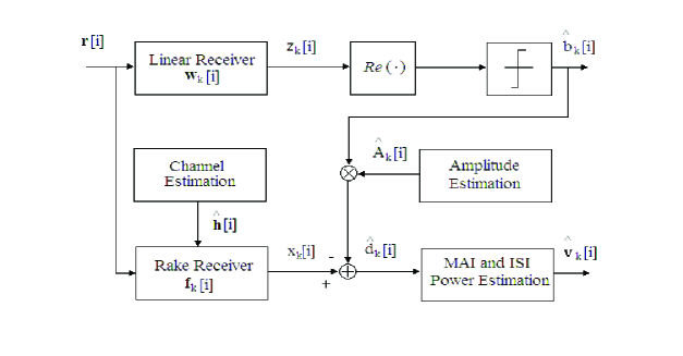
Figure 1: Block diagram of the proposed interference estimation and tracking algorithm.

Channel Estimation:

Let us first present a simple channel estimation algorithm for designing the RAKE receiver. Consider the constraint matrix ${\bf C}_{k}$ that contains one-chip shifted versions of the signature sequence for user $k$ defined in (2) and the assumption that the symbols $b_{k}[i]$ are independent and identically distributed (i.i.d) and statistically independent from the symbols of the other users. The proposed channel estimation algorithm is based on the following cost function

$$\begin{split}{\mathcal{C}}(\hat{\bf h}[i],\hat{A}_{k}[i])&=E\big{[}||\hat{A}_{k}[i]b_{k}[i]{\bf C}_{k}\hat{\bf h}[i]-{\bf r}[i]||^{2}\big{]}\\ &=E\big{[}||\hat{A}_{k}[i]b_{k}[i]\hat{\bf f}_{k}[i]-{\bf r}[i]||^{2}\big{]},\end{split}$$ (27)

where $\hat{\bf h}[i]$ is an estimate of the channel ${\bf h}[i]$ and $\hat{\bf f}_{k}[i]={\bf C}_{k}\hat{\bf h}[i]$ is the RAKE receiver for user $k$ with the estimated channel. By taking the gradient terms of (27), making them equal to zero, we can devise a stochastic gradient (SG) channel estimation algorithm as follows:

$$\hat{\bf h}[i+1]=\hat{\bf h}[i]-\mu_{h}\hat{A}_{k}[i]{\bf C}_{k}^{H}b_{k}^{*}[i]\big{(}b_{k}[i]{\bf C}_{k}\hat{\bf h}[i]-{\bf r}[i]\big{)}.$$ (28)

Amplitude Estimation:

The amplitude has also to be estimated at the receiver in order to provide this information for different tasks such as interference cancellation and power control. The proposed interference estimation and tracking algorithm needs some form of amplitude estimation in order to proceed with the estimation of the interference power. To estimate the amplitudes of the associated user signals, we describe the following optimization problem with the cost function in (27)

$$\begin{split}{\hat{A}}_{k}[i]&=\arg\min_{{A}_{k}[i]}{\mathcal{C}}(\hat{\bf h}[i],\hat{A}_{k}[i])\\ &=\arg\min_{{A}_{k}[i]}E[||{A}_{k}[i]\hat{b}_{k}[i]{\bf C}_{k}\hat{\bf h}[i]-{\bf r}[i]||^{2}].\end{split}$$ (29)

In order to solve the problem above efficiently we describe a simple SG algorithm to estimate the amplitude of user $k$, as given by

$$\begin{split}{\hat{A}}_{k}[i+1]&={\hat{A}}_{k}[i]-\mu_{A}b_{k}^{*}[i]\hat{\bf h}^{H}[i]{\bf C}_{k}^{H}\Big{(}{\hat{A}}_{k}[i]b_{k}[i]{\bf C}_{k}\hat{\bf h}[i]-{\bf r}[i]\Big{)}.\end{split}$$ (30)

Interference Estimation and Tracking:

Let us consider the RAKE receiver with perfect channel knowledge, whose parameter vector ${\bf f}_{k}[i]={\bf C}_{k}{\bf h}[i]$ for user $k$ (desired one) estimates the effective signature sequence at the receiver, i.e. ${\bf C}_{k}{\bf h}[i]=\tilde{\bf s}_{k}[i]$. The output of the RAKE receiver is given by:

$$\begin{split}x_{k}[i]={\bf f}_{k}^{H}[i]{\bf r}[i]&=\underbrace{A_{k}[i]b_{k}[i]{\bf f}_{k}^{H}[i]\tilde{\bf s}_{k}[i]}_{\rm desired~{}signal}+\underbrace{\sum_{\begin{subarray}{c}j=2\\ j\neq k\end{subarray}}^{K}A_{j}[i]b_{j}[i]{\bf f}_{j}^{H}[i]\tilde{\bf s}_{j}[i]}_{\rm MAI}\\ &\quad+\underbrace{{\bf f}_{k}^{H}[i]\boldsymbol{\eta}[i]}_{\rm ISI}+\underbrace{{\bf f}_{k}^{H}[i]{\bf n}[i]}_{\rm noise},\end{split}$$ (31)

where ${\bf f}_{k}^{H}[i]\tilde{\bf s}_{k}[i]=\rho_{k}[i]$ and ${\bf f}_{k}^{H}[i]\tilde{\bf s}_{j}[i]=\rho_{1,j}[i]$ for $j\neq 1$. The symbol $\rho_{k}$ represents the cross-correlation (or inner product) between the effective signature and the RAKE with perfect channel estimates. The symbol $\rho_{1,j}[i]$ represents the cross-correlation between the RAKE receiver and the effective signature of user $j$. The second-order statistics of the output of the RAKE in (31) are described by:

$$\begin{split}E[|x_{k}[i]|^{2}]&=A_{k}^{2}[i]\rho_{p}^{2}[i]\underbrace{E[|b_{k}[i]|^{2}]}_{\rightarrow 1}\\ &\quad+\underbrace{\sum_{\begin{subarray}{c}j=1\\ j\neq k\end{subarray}}^{K}~{}~{}\sum_{\begin{subarray}{c}l=1\\ j\neq k\end{subarray}}^{K}A_{j}^{2}[i]E[b_{j}[i]b_{l}^{*}[i]]{\bf f}_{j}^{H}\tilde{\bf s}_{j}\tilde{\bf s}_{l}^{H}{\bf f}_{j}}_{\rightarrow\sum_{j=1,j\neq k}^{K}{\bf f}_{j}^{H}\tilde{\bf s}_{j}\tilde{\bf s}_{j}^{H}[i]{\bf f}_{j}}\\ &\quad+{{\bf f}_{k}^{H}E[\boldsymbol{\eta}[i]\boldsymbol{\eta}^{H}[i]]{\bf f}_{k}}+\underbrace{{\bf f}_{k}^{H}E[{\bf n}[i]{\bf n}^{H}[i]]{\bf f}_{k}}_{\rightarrow\sigma^{2}{\bf f}_{k}^{H}{\bf f}_{k}}.\end{split}$$ (32)

From the analysis above, we conclude that through the second-order statistics one can identify the sum of the power levels of MAI, ISI and the noise terms. Therefore, our strategy is to obtain instantaneous estimates of the MAI, the ISI and the noise from the output of a RAKE receiver, subtract the detected symbol in (3) from this output (using the more reliable multiuser receiver (${\bf w}_{k}[i]$)) and to track the interference (MAI + ISI + noise) power as shown in Fig. 2. Let us define the difference between the output of the RAKE receiver and the detected symbol for user $1$:

$$\begin{split}d_{k}[i]=x_{k}[i]-\hat{A}_{k}[i]\hat{b}_{k}[i]&\approx\underbrace{\sum_{k=2}^{K}A_{k}[i]b_{k}[i]{\bf f}_{k}^{H}[i]\tilde{\bf s}_{k}[i]}_{\rm MAI}+\underbrace{{\bf f}_{k}^{H}[i]\boldsymbol{\eta}[i]}_{\rm ISI}\\ &+\underbrace{{\bf f}_{k}^{H}[i]{\bf n}[i]}_{\rm noise}.\end{split}$$ (33)

By taking expectations on $|d_{k}[i]|^{2}$ and taking into account the assumption that MAI, ISI and noise are uncorrelated we have:

$$\begin{split}E[|d_{k}[i]|^{2}]&\approx\sum_{k=2}^{K}{\bf f}_{k}^{H}[i]\tilde{\bf s}_{k}[i]\tilde{\bf s}_{k}^{H}[i]{\bf f}_{k}[i]\\ &+{{\bf f}_{k}^{H}[i]E[\boldsymbol{\eta}[i]\boldsymbol{\eta}^{H}[i]]}{\bf f}_{k}[i]+\sigma^{2}{\bf f}_{k}^{H}[i]{\bf f}_{k}[i],\end{split}$$ (34)

where the above equation represents the interference power. Based on time averages of the instantaneous values of the interference power, we introduce the following algorithm to estimate and track $E[|d_{k}[i]|^{2}]$:

$$\hat{v}[i+1]=(1-\beta)\hat{v}[i]+\beta|d_{k}[i]|^{2},$$ (35)

where $\beta$ is a forgetting factor. To incorporate parameter dependency and interference power for computing a more effective bound, we propose the parameter and interference dependent bound (PIDB):

$$\gamma_{k}[i+1]=(1-\beta)\gamma_{k}[i]+\beta\Big{(}\sqrt{\tau~{}{\hat{v}}^{2}[i]}+\sqrt{\alpha||{\bf w}_{k}||^{2}{\hat{\sigma}}^{2}_{v}[i]}\Big{)},$$ (36)

where ${\hat{v}}[i]$ is the estimated interference power in the multiuser system and $\tau$ is a weighting parameter that must be set. Similarly to (26), the equations in (35) and (36) are time-averaged recursions that are aimed at tracking the quantities $|d_{k}[i]|^{2}$ and $(\sqrt{\tau\hat{v}^{2}[i]}+\sqrt{\alpha||{\bf w}_{k}||^{2}\hat{\sigma_{v}}^{2}[i]})$, respectively. The equations in (35) and (36) also avoid undesirable too high or low instantaneous values which may lead to inappropriate time-varying bound $\gamma_{k}[i]$.

V Analysis of The Algorithms

In this section we analyze the channel estimation and interference estimation algorithms described in the previous section. We focus on the convergence properties of the algorithms in terms of the step size parameters $\mu_{h}$, $\mu_{A}$ and $\beta$ used for the channel, the amplitude and the interference power estimators, respectively.

V-A Channel Estimator

In order to analyze the SG channel estimator given in (28), let us first define an error vector $\boldsymbol{\epsilon}_{h}[i]=\hat{\bf h}[i]-{\bf h}_{opt}$. By subtracting ${\bf h}_{opt}$ from the SG recursion in (28), we get

$$\begin{split}\boldsymbol{\epsilon}_{h}[i+1]&=\boldsymbol{\epsilon}_{h}[i]-\mu_{h}\hat{A}_{k}[i]{\bf C}_{k}^{H}b_{k}^{*}[i]\big{(}\hat{A}_{k}[i]b_{k}[i]{\bf C}_{k}\hat{\bf h}[i]\\ &\quad-{\bf r}[i]\big{)}\\ \quad&=\boldsymbol{\epsilon}_{h}[i]-\mu_{h}\hat{A}_{k}[i]b_{k}^{*}[i]{\bf C}_{k}^{H}\big{(}\hat{A}_{k}[i]b_{k}[i]{\bf C}_{k}(\boldsymbol{\epsilon}_{h}[i]+{\bf h}_{opt})\\ &\quad-{\bf r}[i]\big{)}\\ \quad&=\big{[}{\bf I}-\mu_{h}\hat{A}_{k}[i]|b_{k}[i]|^{2}{\bf C}_{k}^{H}{\bf C}_{k}\big{]}\boldsymbol{\epsilon}_{h}[i]\\ &\quad-\mu_{h}\hat{A}_{k}[i]b_{k}^{*}[i]{\bf C}_{k}^{H}\big{(}\hat{A}_{k}[i]b_{k}[i]{\bf C}_{k}{\bf h}_{opt}-{\bf r}[i]\big{)}\\ &=\big{[}{\bf I}-\mu_{h}\hat{A}_{k}[i]|b_{k}[i]|^{2}{\bf C}_{k}^{H}{\bf C}_{k}\big{]}\boldsymbol{\epsilon}_{h}[i]\\ &\quad-\mu_{h}\hat{A}_{k}[i]b_{k}^{*}[i]{\bf C}_{k}^{H}{\bf e}_{k,\textrm{opt}}[i].\end{split}$$ (37)

By considering that the error vector $\boldsymbol{\epsilon}_{h}[i]$, ${\bf e}_{k,\textrm{opt}}[i]$, the signal components $\sum_{k=1}^{K}{\bf x}_{k}[i]$ from the data vector ${\bf r}[i]=\sum_{k=1}^{K}{\bf x}_{k}[i]+{\bf n}[i]$ given by (1) and ${\bf n}[i]$ are statistically independent and computing the covariance matrix of the error vector, i.e. ${\bf K}[i]=E\big{[}\boldsymbol{\epsilon}_{h}[i]\boldsymbol{\epsilon}_{h}^{H}[i]\big{]}$, we obtain

$$\begin{split}{\bf K}[i+1]&=\big{[}{\bf I}-\mu_{h}\sigma_{A_{k}}^{2}\sigma_{b}^{2}{\bf C}_{k}^{H}{\bf C}_{k}\big{]}{\bf K}[i]\big{[}{\bf I}-\mu_{h}\sigma_{A_{k}}^{2}\sigma_{b}^{2}{\bf C}_{k}^{H}{\bf C}_{k}\big{]}\\ &\quad+\mu_{h}^{2}\sigma_{A_{k}}^{2}\sigma_{b}^{2}||{\bf C}_{k}^{H}{\bf C}_{k}||^{2}\textrm{MSE}_{min},\end{split}$$ (38)

where $\sigma_{b}=E[|b_{k}[i]|^{2}]$, $\sigma_{A_{k}}^{2}=E[|A_{k}[i]|^{2}]$ and $\textrm{MSE}_{min}=E[||{\bf e}_{k,\textrm{opt}}[i]||^{2}]$ stands for the minimum MSE achieved by the estimator. The recursive rule/algorithm in (28) is asymptotically unbiased and will converge to the optimum channel estimator ${\bf h}_{\textrm{o}pt}$ if the step size $\mu_{h}$ satisfies the following condition

$$0<\mu_{h}<\frac{2}{\sigma_{b}^{2}\sigma_{A_{k}}^{2}\lambda_{max}},$$ (39)

where $\lambda_{max}$ is the largest eigenvalue of the matrix ${\bf C}_{k}^{H}{\bf C}_{k}$. The condition above with concern to the step size $\mu_{h}$ arises from difference equations. The quantities generated in (38) represent a geometric series with a geometric ratio equal to $(1-\mu_{h}\sigma_{A_{k}}^{2}\sigma_{b}^{2}{\bf C}_{k}^{H}{\bf C}_{k})$. For stability or convergence of this algorithm, the magnitude of this geometric ratio must be less than $1$ for all $k$ ($|1-\mu_{h}\sigma_{A_{k}}^{2}\sigma_{b}^{2}{\bf C}_{k}^{H}{\bf C}_{k}|<1$). This means that $0<\mu_{h}<\frac{2}{\sigma_{b}^{2}\sigma_{A_{k}}^{2}\lambda_{max}}$. The reviewer is referred to [2, 24] for further details.

V-B Amplitude Estimator

In order to analyze the SG amplitude estimator described in (30), let us first define an error signal $\epsilon_{A,k}[i]=\hat{A}_{k}[i]-A_{k,opt}$. By subtracting $A_{k,opt}$ from the equation in (30) we obtain

$$\begin{split}\epsilon_{A_{k}}[i+1]&=\epsilon_{A_{k}}[i]-\mu_{A}b_{k}^{*}[i]\hat{\bf h}^{H}[i]{\bf C}_{k}^{H}\big{(}\hat{A}_{k}[i]b_{k}[i]{\bf C}_{k}\hat{\bf h}[i]-{\bf r}[i]\big{)}\\ &=\epsilon_{A_{k}}[i]-\mu_{A}b_{k}^{*}[i]\hat{\bf h}^{H}[i]{\bf C}_{k}^{H}\big{(}(\epsilon_{A,k}[i]\\ &\quad+A_{k,opt})b_{k}[i]{\bf C}_{k}\hat{\bf h}[i]-{\bf r}[i]\big{)}\\ &=\epsilon_{A_{k}}[i]-\mu_{A}|b_{k}[i]|^{2}\hat{\bf h}[i]{\bf C}_{k}^{H}{\bf C}_{k}\hat{\bf h}[i]\epsilon_{A_{k}}[i]\\ &\quad-\mu_{A}b_{k}^{*}[i]\hat{\bf h}^{H}[i]{\bf C}_{k}^{H}\big{(}A_{k,opt}b_{k}[i]{\bf C}_{k}\hat{\bf h}[i]-{\bf r}[i]\big{)}\\ &=\big{(}1-\mu_{A}|b_{k}[i]|^{2}\hat{\bf h}[i]{\bf C}_{k}^{H}{\bf C}_{k}\hat{\bf h}[i]\big{)}\epsilon_{A_{k}}[i]\\ &\quad-\mu_{A}b_{k}^{*}[i]\hat{\bf h}^{H}[i]{\bf C}_{k}^{H}e_{A,\textrm{opt}}[i].\end{split}$$ (40)

By considering that the error $\epsilon_{A}[i]$, ${\bf e}_{A,\textrm{opt}}[i]=A_{k,opt}b_{k}[i]{\bf C}_{k}\hat{\bf h}[i]-{\bf r}[i]$, the signal components $\sum_{k=1}^{K}{\bf x}_{k}[i]$ from the data vector ${\bf r}[i]=\sum_{k=1}^{K}{\bf x}_{k}[i]+{\bf n}[i]$ given by (1) and ${\bf n}[i]$ are statistically independent, and by computing the mean-squared error, i.e., $\textrm{MSE}(A_{k}[i])[i]=K_{A_{k}}[i]=E[|\epsilon[i]|^{2}]$, we get

$$\begin{split}\textrm{MSE}(A_{k}[i])[i+1]&=\big{(}1-\mu_{A}\sigma_{b}^{2}E[||{\bf h}_{k}^{H}[i]{\bf C}_{k}^{H}||^{2}]\big{)}^{2}K_{A_{k}}[i]\\ &\quad+\mu_{A}^{2}\sigma_{b}^{2}E[||{\bf h}_{k}^{H}[i]{\bf C}_{k}^{H}||^{2}]\textrm{MSE}_{A,min},\end{split}$$ (41)

where $\textrm{MSE}_{A,min}=E[||{e}_{A,\textrm{opt}}[i]||^{2}]$. The cross multiplication between the terms will vanish as a result of the statistical independence between them. The general algorithm in (30) will converge asymptotically and in an unbiased way to the $A_{k,opt}$ provided the step size $\mu_{A}$ is chosen such that

$$0<\mu_{A}<\frac{2}{\sigma_{b}^{2}E[||{\bf h}_{k}^{H}[i]{\bf C}_{k}^{H}||^{2}]}.$$ (42)

The above range of values has to be tuned in order to ensure good convergence and tracking of the amplitude.

V-C Interference Estimation and Tracking Algorithm

Let us describe in a general form the mechanisms for interference estimation and tracking given in (26) and (36). We can write without loss of generality

$$\gamma_{k}[i+1]=(1-\beta)\gamma_{k}[i]+\beta~{}\textrm{Po}[i],$$ (43)

where $\textrm{Po}[i]$ can account either for a parameter dependent bound (PDB), as described in Section IV. A, or for a parameter and interference dependent bound (PIDB), as the one detailed in Section IV.B.

Our goal is to establish the convergence of a general stochastic recursion, as the one given in (43), in terms of the mean-squared error (MSE) at iteration $[i]$, as described by

$$\textrm{MSE}(\gamma[i])[i]=E\big{[}|\gamma_{k}[i]-\gamma_{k,\textrm{opt}}|^{2}\big{]},$$ (44)

where $\gamma_{k,\textrm{opt}}$ is the optimal parameter estimate for $\gamma_{k}[i]$.

We will show that under certain conditions on $\beta$, the sequence converges to the optimal $\gamma_{k,\textrm{opt}}$ in the mean-square sense. Let us define the error

$$\epsilon_{\gamma}[i]=\gamma_{k}[i]-\gamma_{k,\textrm{opt}},$$

and substitute the above equation into (44), which yields

$$\begin{split}\epsilon_{\gamma}[i+1]&=(1-\beta)\epsilon_{\gamma}[i]+\beta(\textrm{Po}[i]-\gamma_{k,\textrm{opt}})\\ &=(1-\beta)\epsilon_{\gamma}[i]+\beta e_{k,\textrm{opt}}[i],\end{split}$$ (45)

The MSE at time instant $[i+1]$ is given by

$$\begin{split}\textrm{MSE}(\gamma[i+1])[i+1]&=\epsilon_{\gamma}^{*}[i+1]\epsilon_{\gamma}[i+1]=|\epsilon_{\gamma}[i+1]|^{2}\\ &=(1-\beta)^{2}\epsilon_{\gamma}^{*}[i]\epsilon_{\gamma}[i]\\ &\quad+\beta^{2}~{}e_{k,\textrm{opt}}[i]e_{k,\textrm{opt}}^{*}[i]\\ &\quad+(1-\beta)\beta~{}\epsilon_{\gamma}[i]e_{k,\textrm{opt}}^{*}[i]\\ &\quad+(1-\beta)\beta~{}\epsilon_{\gamma}^{*}[i]e_{k,\textrm{opt}}[i].\end{split}$$ (46)

By taking the expected value on both sides and assuming that $\epsilon_{\gamma}[i]$ and $e_{k,\textrm{opt}}[i]$ are statistically independent we have

$$\begin{split}E\big{[}\textrm{MSE}[i+1]\big{]}&=E\big{[}|\epsilon_{\gamma}[i+1]|^{2}\big{]}\\ &=K_{\gamma}[i+1]\\ &=(1-\beta)K_{\gamma}[i](1-\beta)+\beta^{2}|e_{k,\textrm{opt}}[i]|^{2},\end{split}$$ (47)

where $|e_{k,\textrm{opt}}[i]|^{2}$ is the minimum MSE achieved by the estimator.

We can notice that the cross-multiplication terms will vanish as a result of the statistical independence between the terms. The general recursive rule in (43) will converge asymptotically provided the step size $\beta$ is chosen such that

$$0<\beta<2.$$ (48)

The above range of values has to be adjusted in order to ensure good convergence and tracking of the parameter dependency and/or the interference modeled here as the quantity $\textrm{Po}[i]$.

VI Simulations

In this section we assess the performance of the proposed and existing adaptive algorithms in several scenarios of practical interest:

• The NLMS, the SM-NLMS [3], the SM-NLMS of Guo and Huang [12] and the proposed SM-NLMS with the parameter-dependent (PDB) and parameter and interference dependent (PIDB) time-varying bounds.

• The AP [2], the SM-AP [4] and the proposed SM-AP with the PDB and PIDB time-varying bounds.

• The BEACON [7] and the proposed BEACON algorithms with the PDB and PIDB time-varying bounds.

We consider for the sake of simplicity binary phase-shift-keying (BPSK) modulation, a DS-CDMA system with Gold sequences of length $N=31$ and typical fading channels found in mobile communications systems that can be modeled according to Clarke’s model [22]. The channels experienced by different users are identical since we focus on a downlink scenario and the desired receiver processes the transmissions intended to other users (MAI) over the same channel as its own signal. The channel coefficients are $h_{l}[i]=p_{l}\alpha_{l}[i]$, where $\alpha_{l}[i]$ ($l=0,1,\ldots,L_{p}-1$) are obtained with Clarke’s model [22]. In particular, we employ standard SG adaptive algorithms for channel estimation and RAKE design in order to concentrate on the comparison between the analyzed algorithms for receiver parameter estimation. We show the results in terms of the normalized Doppler frequency $f_{d}T$ (cycles/symbol) and use three-path channels with relative powers given by $0$, $-3$ and $-6$ dB, where in each run the spacing between paths is obtained from a discrete uniform random variable between $1$ and $2$ chips. The channel coefficients $h_{l}[i]$ ($l=0,1,\ldots,L_{p}-1$) are constant during each symbol interval and change according to Clarke’s model over time. Since the channel is modelled as an FIR filter, we employ a channel estimation filter with $6$ taps as an upper bound for the experiments. Note that the delays of the channel taps are multiples of the chip rate and are random. Their range coincides with the maximum length of the estimation filter which is $6$ taps.

The parameters of the algorithms are optimized and shown for each example, the system has a power distribution for the interferers that follows a log-normal distribution with associated standard deviation of $3$ dB and experiments are averaged over $100$ independent runs. The receivers are trained with $200$ symbols and then switch to decision-directed mode for each data packet. We address the dynamic channel by adjusting the receiver weights with the training sequences (with length equal to $200$ symbols) and then we exploit the decision-directed mode to track the channel variations. If the channel does not vary too fast then the adaptive receivers can track it with this scheme, as will be shown in what follows.

VI-A Interference Estimation and Tracking

In order to evaluate the effectiveness of the proposed interference estimation and tracking algorithms, that are incorporated into the time-varying error bounds for tracking the MAI and ISI powers, we carried out an experiment, depicted in Fig. 2. In this scenario, the proposed algorithm estimates of the MAI and ISI powers are compared to the actual interference power levels that are generated by the simulations. The results obtained show that the proposed algorithms are very effective for estimating and tracking the interference power in dynamic environments. Specifically, the estimation error does not exceed in average $5\%$ of the estimated power level, as depicted in Fig. 2. Indeed, the algorithms are capable of accurately estimating the interference power levels and tracking them, which can be verified by the proximity between the curves obtained with the estimation algorithms and the actual values.

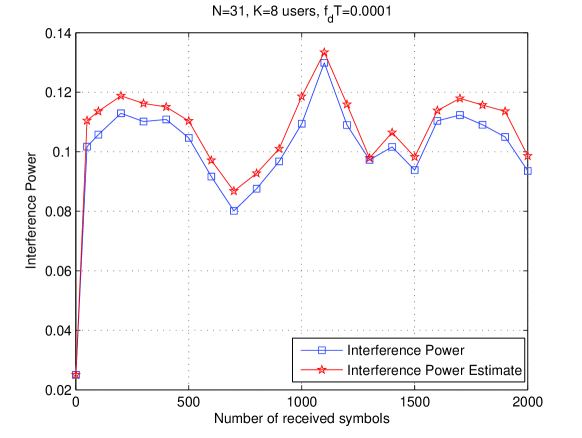
Figure 2: Performance of the interference power estimation and tracking at $E_{b}/N_{0}=12$ dB and with $\beta=0.05$ .

VI-B SINR Performance

In this part, the performance of the proposed algorithms is assessed in terms of output signal-to-interference-plus-noise ratio (SINR), which is defined as

$$\centering{\rm SINR}[i]=\frac{{\boldsymbol{w}}^{H}[i]{\boldsymbol{R}}_{s}[i]{\boldsymbol{w}}[i]}{{\boldsymbol{w}}^{H}[i]{\boldsymbol{R}}_{I}[i]{\boldsymbol{w}}[i]},\@add@centering$$ (49)

where ${\boldsymbol{R}}_{s}[i]$ is the autocorrelation matrix of the desired signal and ${\boldsymbol{R}}_{I}[i]$ is the cross-correlation matrix of the interference and noise in the environment. The goal here is to evaluate the convergence performance of the proposed algorithms with time-varying error bounds for the modified SM-NLMS, SM-AP and BEACON techniques. Specifically, we consider examples where the adaptive receivers converge to about the same level of SINR, which illustrates in a fair way the speed of convergence of the proposed algorithms and the existing ones. We also measure the update rate (UR) of all the SM-based algorithms as an important complexity issue.

The SINR convergence performance of NLMS, AP and BEACON algorithms is illustrated via computer experiments in Figs. 3, 4 and 5, respectively. The curves in Fig. 3 show that the proposed SM-NLMS algorithms with the PIDB time-varying error bounds achieve the fastest convergence, followed by the proposed SM-NLMS-PDB, the SM-NLMS-Huang [12], the conventional SM-NLMS [3] and the NLMS [2] recursions. Even though the proposed SM-NLMS-PIDB and SM-NLMS-PDB algorithms enjoy the fastest convergence rates, they exhibit remarkably lower UR properties, saving significant computational resources and being substantially more economical than the conventional SM-NLMS algorithm.

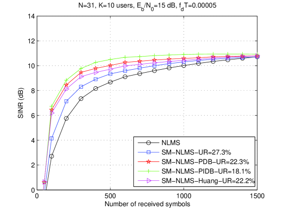
Figure 3: SINR Performance of NLMS algorithms at $E_{b}/N_{0}=15$ dB with $\beta=0.05$, $\alpha=8$ and $\tau=2$ .

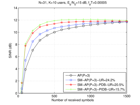
Figure 4: SINR Performance of AP algorithms at $E_{b}/N_{0}=15$ dB with $\beta=0.05$, $\alpha=8$ and $\tau=2$ .

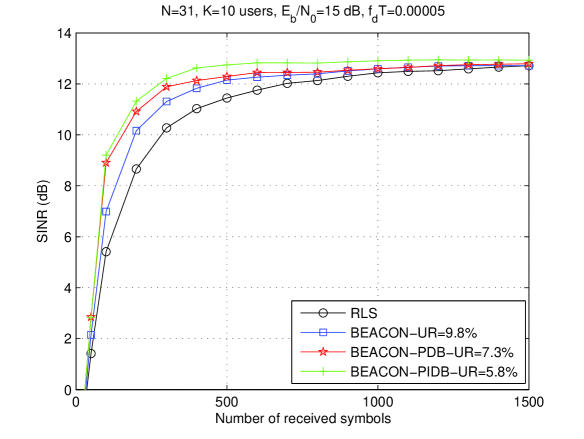
Figure 5: SINR Performance of RLS and BEACON algorithms at $E_{b}/N_{0}=15$ dB with $\beta=0.05$, $\alpha=5$ and $\tau=1.5$ .

By observing the results for the AP and the BEACON algorithms, shown in Figs. 4 and 5, one can notice that the results corroborate those found for the NLMS algorithms. It should be noted that despite their higher complexity than NLMS algorithms, the AP and BEACON techniques have faster convergence, better SINR steady-state performance and lower URs.

VI-C BER Performance

In this subsection, we focus on the bit error rate (BER) performance of the proposed algorithms. We consider a simulation setup where the data packets transmitted have $1500$ symbols and the adaptive receivers and algorithms are trained with $200$ symbols and then switch to decision-directed mode, in which they continue to adapt and track the channel variations.

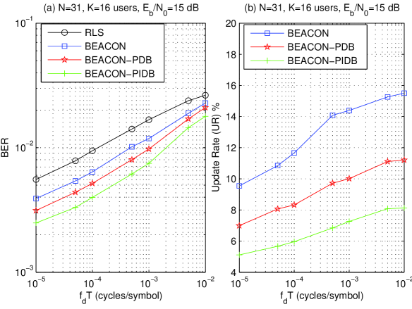
Figure 6: (a) BER performance versus $f_{d}T$ and (b) Update Rate (UR) versus $f_{d}T$ for the BEACON algorithms for a forgetting factor $\lambda=0.997$ for the conventional RLS algorithm. The proposed BEACON-PDB abd BEACON-PIDB algorithms use $\beta=0.05$, $\alpha=5$ and $\tau=1.5$.

Firstly, we consider a study of the BER performance and the impact on the UR of the fading rate of the channel ($f_{d}T$) in the experiment shown in Fig. 6. We observe from the curves in Fig. 6 (a) that the new BEACON algorithms obtain substantial gains in BER performance over the original BEACON [7] and the RLS algorithm [2] for a wide range of fading rates. In addition, as the channel becomes more hostile the performance of the analyzed algorithms approaches one another, indicating that the adaptive techniques are encountering difficulties in dealing with the changing environment and interference. With regard to the UR, the curves in Fig. 6 (b) illustrate the impact of the fading rate on the UR of the algorithms. Indeed, it is again verified that the proposed BEACON-PDB and BEACON-PIDB algorithms can obtain significant savings in terms of UR, allowing the mobile receiver to share its processing power with other important functions and to save battery life.

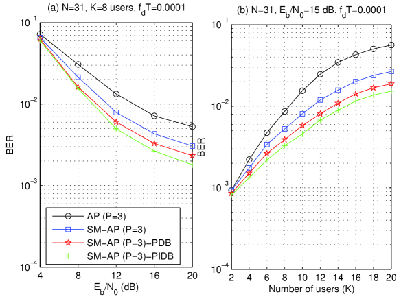
Figure 7: BER performance versus (a) $E_{b}/N_{0}$ dB (b) $K$ for AP algorithms with $P=3$.

The BER performance versus the signal-to-noise ratio ($E_{b}/N_{0}$) and the number of users (K) is illustrated in Figs. 7 for the AP with $P=3$. The results confirm the excellent performance of the proposed PIDB time-varying error bound for a variety of scenarios, algorithms and loads. The PIDB technique allows significantly superior performance while reducing the UR of the algorithm and saving computations. We can also notice that significant performance and capacity gains can be obtained by exploiting data reuse. From the curves it can be seen that the proposed PIDB mechanism with the SM-AP with $P=3$ can save up to $3$ dB and up to $4$ dB as compared to the PDB and to the SM-AP with fixed bounds, respectively, for the same BER performance. In terms of system capacity, we verify that the PIDB approach can accommodate up to $4$ more users as compared to the PDB technique for the same BER performance.

VII Conclusions

We proposed SM adaptive algorithms based on time-varying error bounds. Adaptive algorithms for tracking MAI and ISI power and taking into account parameter dependency were incorporated into the new time-varying error bounds. Simulations show that the new algorithms outperform previously reported techniques and exhibit a reduced number of updates. The proposed algorithms can have a significant impact on the design of low-complexity receivers for spread spectrum systems, as well as for future MIMO systems employing either CDMA or OFDM as the multiple access technology. The proposed algorithms are especially relevant to future wireless cellular, ad hoc and sensor networks, where their potential to save computational resources may play a significant role given the limited battery resources and processing capabilities of mobile units and sensors.

References

- [1]
- [2] P. S. R. Diniz, Adaptive Filtering: Algorithms and Practical Implementations, 2nd edition, Kluwer Academic Publishers, Boston, MA, 2002.
- [3] S. Gollamudi, S. Nagaraj, S. Kapoor and Y. F. Huang, “Set-Membership Filtering and a Set-Membership Normalized LMS Algorithm with an Adaptive Step Size,” IEEE Sig. Proc. Letters, vol. 5, No. 5, May 1998.
- [4] S. Werner and P. S. R. Diniz, “Set-membership affine projection algorithm”, IEEE Sig. Proc. Letters, vol 8., no. 8, August 2001.
- [5] P. S. R. Diniz and S. Werner, “Set-Membership Binormalized Data Re-using LMS Algorithms,” IEEE Trans. Sig. Proc., vol. 51, no. 1, pp. 124-134, January 2003.
- [6] S. Gollamudi, S. Kapoor, S. Nagaraj and Y. F. Huang, “Set-Membership Adaptive Equalization and an Updator-Shared Implementation for Multiple Channel Communication Systems”, IEEE Transactions on Signal Processing, vol. 46, no. 9, pp. 2372-2385, September 1998.
- [7] S. Nagaraj, S. Gollamudi, S. Kapoor and Y. F. Huang, “BEACON: an adaptive set-membership filtering technique with sparse updates”, IEEE Transactions on Signal Processing, vol. 47, no. 11, November 1999.
- [8] S. Nagaraj, S. Gollamudi, S. Kapoor, Y. F. Huang and J. R. Deller Jr., “Adaptive Interference Suppression for CDMA Systems with a Worst-Case Error Criterion,” IEEE Transactions on Signal Processing, vol. 48, No. 1, January 2000.
- [9] I. Akyildiz, W. Su, Y. Sankarasubramaniam, and E. Cayirci, ”A survey on sensor networks,” IEEE Communications Magazine, vol. 40, Issue 8, August, 2002, pp. 102-114.
- [10] D. Maksarov and J. P. Norton, “Tuning of noise bounds in parameter set estimation,” in Proceedings of International Conference on Identification in Engineering Systems, Swansea, UK, 27-29, March 1996, pp. 584-593.
- [11] S. Gazor and K. Shahtalebi, “A New NLMS Algorithm for Slow Noise Magnitude Variation”, IEEE Signal Processing Letters, vol. 9, no. 11, November 2002.
- [12] L. Guo and Y. F. Huang, “Set-Membership Adaptive Filtering with Parameter-Dependent Error Bound Tuning,” IEEE Proc. Int. Conf. Acoust. Speech and Sig. Proc., 2005.
- [13] L. Guo and Y. F. Huang, “Frequency-Domain Set-Membership Filtering and Its Applications”, IEEE Transactions on Signal Processing, Vol. 55, No. 4, April 2007, pp. 1326-1338.
- [14] T. M. Lin, M. Nayeri and J. R. Deller, Jr., “Consistently Convergent OBE Algorithm with Automatic Selection of Error Bounds,” International Journal of Adaptive Control and Signal Processing, vol. 12, pp. 302-324, June 1998.
- [15] J. R. Deller, S. Gollamudi, S. Nagaraj, and Y. F. Huang, “Convergence analysis of the QUASI-OBE algorithm and the performance implications,” in Proc. IFAC Int. Symp. Syst. Ident., vol. 3, Santa Barbara, CA, June 2000, pp. 875-880.
- [16] S. Dasgupta and Y. F. Huang, “Asymptotically convergent modified recursive least-squares with data dependent updating and forgetting factor for systems with bounded noise,” IEEE Trans. Inform. Theory, vol. IT-33, pp. 383–392, 1987.
- [17] J. R. Deller, M. Nayeri, and M. Liu, “Unifying the landmark developments in optimal bounding ellipsoid identification,” Int. J. Adap. Contr. Signal Process., vol. 8, pp. 43–60, 1994.
- [18] D. Joachim, J. R. Deller, and M. Nayeri, “Multiweight optimization in OBE algorithms for improved tracking and adaptive identification,” in Proc. IEEE Int. Acoust., Speech Signal Process., vol. 4, Seattle, WA, May 1998, pp. 2201-2204.
- [19] M. L. Honig and H. V. Poor, “Adaptive interference suppression,” in Wireless Communications: Signal Processing Perspectives, H. V. Poor and G. W. Wornell, Eds. Englewood Cliffs, NJ: Prentice-Hall, 1998, Chapter 2, pp. 64-128.
- [20] R.C. de Lamare, R. Sampaio-Neto, “Minimum Mean-Squared Error Iterative Successive Parallel Arbitrated Decision Feedback Detectors for DS-CDMA Systems”, IEEE Transactions on Communications, vol. 56, no. 5, May 2008, pp. 778 - 789.
- [21] S. Haykin, Adaptive Filter Theory, 4rd edition, Prentice-Hall, Englewood Cliffs, NJ, 2002.
- [22] T. S. Rappaport, Wireless Communications, Prentice-Hall, Englewood Cliffs, NJ, 1996.
- [23] Third Generation Partnership Project (3GPP), specifications 25.101, 25.211-25.215, versions 5.x.x.
- [24] D. P. Bertsekas, Nonlinear Programming, Athena Scientific, 2nd Ed., 1999.
- [25] A. Klein, G. Kaleh, and P. Baier, “Zero forcing and minimum mean- square-error equalization for multiuser detection in code-divisionmultiple-access channels,” IEEE Trans. Vehicular Technology, vol. 45, no. 2, pp. 276–287, 1996.
- [26] S. Buzzi and H. V. Poor, “Channel estimation and multiuser detection in long-code DS/CDMA systems,” IEEE Journal on Selected Areas in Communications, vol. 19, no. 8, pp. 1476– 1487, 2001.
- [27] Z. Xu and M. Tsatsanis, “Blind channel estimation for long code multiuser CDMA systems,” IEEE Trans. Signal Processing, vol. 48, no. 4, pp. 988–1001, 2000.
- [28] P. Liu and Z. Xu, “Joint performance study of channel estimation and multiuser detection for uplink long-code CDMA systems,” EURASIP Journal on Wireless Communications and Networking: Special Issue on Innovative Signal Transmission and Detection Techniques for Next Generation Cellular CDMA System, vol. 2004, no. 1, pp. 98-112, August 2004.
- [29] R. C. de Lamare and R. Sampaio-Neto, “Reduced-Rank Adaptive Filtering Based on Joint Iterative Optimization of Adaptive Filters, ” IEEE Signal Processing Letters, Vol. 14 No. 12, December 2007, pp. 980 - 983.
- [30] R. C. de Lamare and R. Sampaio-Neto, “Adaptive Reduced-Rank Processing Based on Joint and Iterative Interpolation, Decimation and Filtering”, IEEE Transactions on Signal Processing, vol. 57, no. 7, July 2009, pp. 2503 - 2514.