Compressed Sensing with Linear Correlation Between Signal and Measurement Noise

Abstract

Existing convex relaxation-based approaches to reconstruction in compressed sensing assume that noise in the measurements is independent of the signal of interest. We consider the case of noise being linearly correlated with the signal and introduce a simple technique for improving compressed sensing reconstruction from such measurements. The technique is based on a linear model of the correlation of additive noise with the signal. The modification of the reconstruction algorithm based on this model is very simple and has negligible additional computational cost compared to standard reconstruction algorithms, but is not known in existing literature. The proposed technique reduces reconstruction error considerably in the case of linearly correlated measurements and noise. Numerical experiments confirm the efficacy of the technique. The technique is demonstrated with application to low-rate quantization of compressed measurements, which is known to introduce correlated noise, and improvements in reconstruction error compared to ordinary Basis Pursuit De-Noising of up to approximately 7 dB are observed for 1 bit/sample quantization. Furthermore, the proposed method is compared to Binary Iterative Hard Thresholding which it is demonstrated to outperform in terms of reconstruction error for sparse signals with a number of non-zero coefficients greater than approximately $\nicefrac{{1}}{{10}}$th of the number of compressed measurements.

1 Introduction

In the recently emerged field of compressed sensing, one considers linear measurements $\mathbf{y}$ of a sparse vector $\mathbf{x}$, possibly affected by noise as:

$$\mathbf{y}=\mathbf{A}\mathbf{x}+\mathbf{n},$$ (1)

where the measurements $\mathbf{y}\in\mathbb{R}^{M\times 1}$, the sparse vector $\mathbf{x}\in\mathbb{R}^{N\times 1}$, the additive noise $\mathbf{n}\in\mathbb{R}^{M\times 1}$, the system matrix $\mathbf{A}\in\mathbb{R}^{M\times N}$, and $M\ll N$ [1, 2, 3]. $\mathbf{A}$ is generally the product of a measurement matrix and a dictionary matrix: $\mathbf{A}=\bm{\Phi}\bm{\Psi}$, where $\bm{\Phi}\in\mathbb{C}^{M\times N}$, $\bm{\Psi}\in\mathbb{C}^{N\times N}$. For simplicity, we assume that $\bm{\Psi}$ is an orthonormal basis although more general dictionaries are indeed possible [4].

The essence of compressed sensing, as Donoho, Candès, Romberg, and Tao show in [1, 2], is that the under-determined equation system (1) can be solved provided that:

1. The vector $\mathbf{x}$ is sparse; i.e., only few ($K$) elements in $\mathbf{x}$ are non-zero.

   $$K=\left|\left\{x_{i}\middle|x_{i}\neq 0,i=1,\ldots,N\right\}\right|$$ (2)

   $\mathbf{x}$ can also be approximated sparsely if it is compressible [3, Sec. 3.3], meaning that its coefficients sorted by magnitude decay rapidly to zero.

2. The system matrix $\mathbf{A}$ obeys the Restricted Isometry Property (RIP) with isometry constant $\delta_{K}>0$, defined as follows:

   $$\left(1-\delta_{K}\right)\left\|\mathbf{x}\right\|_{\ell_{2}}^{2}\leq\left\|\mathbf{A}\mathbf{x}\right\|_{\ell_{2}}^{2}\leq\left(1+\delta_{K}\right)\left\|\mathbf{x}\right\|_{\ell_{2}}^{2},$$ (3)

   for any at most $K$-sparse vector $\mathbf{x}$ such that [5]:

   $$\delta_{K}+\delta_{2K}+\delta_{3K}<1.$$ (4)

   This holds with high probability when $\bm{\Phi}$ is generated with zero-mean independent identically distributed (i.i.d.) Gaussian entries with variance $\frac{1}{M}$. Note that (3) and (4) are sufficient but not necessary conditions, and rather conservative conditions indeed, as shown in [6].

   Conditions (3) and (4) lead to the following sufficient amount of measurements $M$ for Gaussian measurement matrices $\bm{\Phi}$ [7]:

   $$M\geq CK\log\left(\frac{N}{M}\right),$$ (5)

   where $C$ is a fairly small constant which can be calculated as a function of $\frac{M}{N}$ [5].

Given the measurements $\mathbf{y}$, the unknown sparse vector $\mathbf{x}$ can be reconstructed by solving the following convex optimization problem [3, Sec. 4]:

$$\hat{\mathbf{x}}=\operatornamewithlimits{argmin}_{\mathbf{u}:\ \|\mathbf{y}-\mathbf{A}\mathbf{u}\|_{2}\leq\epsilon}\|\mathbf{u}\|_{1},$$ (6)

where the fidelity constraint $\|\mathbf{y}-\mathbf{A}\mathbf{u}\|_{2}\leq\epsilon$ ensures consistency with the observed measurements to within some margin of error, $\epsilon$, which is chosen sufficiently large to accommodate the error $\mathbf{n}$ and/or approximation error in the case of compressible signals. The form of the optimization problem in (6) is known as Least Absolute Shrinkage and Selection Operator (LASSO) [8] or Basis Pursuit De-Noising (BPDN) [9] and also comes in other variants such as the Dantzig selector [10]. In addition to the convex optimization approach to reconstruction in compressed sensing, there exist several iterative/greedy algorithms such as Iterative Hard Thresholding (IHT) [11], or Subspace Pursuit (SP) [12] and Compressive Sampling Matching Pursuit (CoSaMP) [13] as well as the more generalized incarnation of the two latter, Two-Stage Thresholding (TST) [14]. We generally refer to such convex or greedy approaches as reconstruction algorithms. The reconstruction algorithms generally assume the noise to be white and independent of the measurements before noise $\bar{}\mathbf{y}=\mathbf{A}\mathbf{x}$. In particular, to the best of the authors’ knowledge, the case of measurement noise being linearly correlated with the measurements has not been treated in the existing literature. Such correlation arises in for example the case of low-resolution quantization. As we demonstrate in Section 2, this case poses a problem for the accuracy of the found solution $\hat{\mathbf{x}}$. More special cases of correlated noise arising from Poisson measurements or quantisation of measurements has, however, been treated in for example [15, 16, 17].

In this paper, we propose a simple yet efficient approach to alleviating the problem of linear correlation between the measurements before noise $\bar{}\mathbf{y}$ and the noise $\mathbf{n}$. Our proposal boils down to a simple scaling of the solution $\hat{\mathbf{x}}$. Through numerical experiments we demonstrate how linearly correlated measurements and noise adversely affect the reconstruction error and demonstrate how our proposal improves the estimates considerably.

As an application example, we demonstrate the proposed approach in the case of low-rate scalar quantization of the measurements $\bar{}\mathbf{y}$ which can be observed to introduce the mentioned linearly correlated measurement noise. We demonstrate how a well-known linear model used for modeling such correlation in scalar quantization is equivalent to the model of correlated measurement noise considered in this work.

The article is structured as follows: Section 2 introduces the considered model of linear correlation between compressed measurements and noise and proposes a solution to enhance reconstruction under these conditions, Section 3 describes simulations conducted to evaluate the performance of the proposed approach compared to a traditional approach, Section 4 presents the results of these numerical simulations, Section 5 provides discussions of some of the presented results, and Section 6 concludes the article.

2 Methodology

2.1 Correlated Measurements and Noise

We consider additive measurement noise $\mathbf{n}$ which is correlated with the measurements before noise $\bar{}\mathbf{y}$. We model the correlation by the linear model:

$$\mathbf{y}=\alpha\mathbf{A}\mathbf{x}+\mathbf{w},$$ (7)

where $\mathbf{w}$ is assumed an additive white noise uncorrelated with $\mathbf{x}$ and $0<\alpha\leq 1$ where $\alpha=1$ covers the ordinary case of uncorrelated measurement noise. $\mathbf{A}$ is the product of a measurement matrix $\bm{\Phi}$ with i.i.d. Gaussian entries $\sim\mathcal{N}\left(0,\frac{1}{M}\right)$ and an orthonormal dictionary matrix $\bm{\Psi}$. The model (7) results in the following additive noise term:

$$\mathbf{n}=\mathbf{y}-\bar{}\mathbf{y}=\alpha\mathbf{A}\mathbf{x}+\mathbf{w}-\mathbf{A}\mathbf{x}=(\alpha-1)\mathbf{A}\mathbf{x}+\mathbf{w}$$ (8)

We define $\bar{}\mathbf{y}=\mathbf{A}\mathbf{x}$ to signify the measurements before introduction of additive noise. It is readily seen from (8) that $\mathbf{n}$ is correlated with $\mathbf{x}$. The noise variance is

$$\sigma_{n}^{2}=\frac{1}{M}\operatorname{\mathbb{E}}\left[\mathbf{n}^{\mathrm{T}}\mathbf{n}\right]=\frac{1}{M}\left((\alpha-1)^{2}\operatorname{\mathbb{E}}\left[\bar{}\mathbf{y}^{\mathrm{T}}\bar{}\mathbf{y}\right]+\operatorname{\mathbb{E}}\left[\mathbf{w}^{\mathrm{T}}\mathbf{w}\right]\right),$$ (9)

which can be calculated by assuming that $\sigma_{\bar{y}}^{2}=\frac{1}{M}\operatorname{\mathbb{E}}\left[\bar{}\mathbf{y}^{\mathrm{T}}\bar{}\mathbf{y}\right]$ and $\sigma_{w}^{2}=\frac{1}{M}\operatorname{\mathbb{E}}\left[\mathbf{w}^{\mathrm{T}}\mathbf{w}\right]$ are known or can be estimated. For example, we show an example for $\sigma_{w}^{2}$ in the case of quantization in Section 2.5, (21).

The specific problem caused by correlated measurements and noise as modeled by (7) is that the noise itself is partly sparse in the same dictionary as the signal of interest, $\mathbf{x}$. Intuitively, this causes a solution $\hat{\mathbf{x}}$ as given by, e.g., (6) to adapt to part of the noise as well as the signal of interest, unless steps are taken to mitigate this effect.

2.2 Proposed Approach

Using the model in (7), we propose the following reconstruction of the sparse vector $\mathbf{x}$ instead of the standard approach in (6). Equation (7) motivates replacing the system matrix $\mathbf{A}$ by its scaled version $\alpha\mathbf{A}$. We exemplify this approach by applying it in the BPDN reconstruction formulation as below. Replacing $\mathbf{A}$ by $\alpha\mathbf{A}$ in the standard approach (6), we arrive at

$$\hat{\mathbf{x}}_{1}=\operatornamewithlimits{argmin}_{\mathbf{u}:\ \|\mathbf{y}-\alpha\mathbf{A}\mathbf{u}\|_{2}\leq\epsilon}\|\mathbf{u}\|_{1}.$$ (10)

Since $\epsilon$ should be chosen to accommodate the level of noise in the measurements $\mathbf{y}$, we can see that, one choice could be to set

$$\epsilon =\|\mathbf{n}\|_{2}$$ (11)

$$\epsilon =\|\mathbf{w}\|_{2}$$ (12)

in (6) or (10), respectively. Since the noise terms $\mathbf{n}$ and $\mathbf{w}$ are assumed unknown, (11) and (12) are not realistic choices of $\epsilon$. The optimal choice of $\epsilon$ is dependent on the true solution $\mathbf{x}$, and is therefore difficult to obtain in practice as exemplified for more general inverse problems in, e.g., [18]. For this reason, various rules of thumb exist for the selection of $\epsilon$. One such choice is found in [19, Sec. 5.3]:

$$\epsilon=\sqrt{M+2\sqrt{2M}}\sigma,$$ (13)

where $\sigma$ is the noise level (standard deviation) of the stochastic error $\mathbf{n}$ or $\mathbf{w}$ in (1) or (7), respectively.

2.3 Additional Insight on the Proposed Approach

As outlined in Section 2.2, the model of the correlation between $\mathbf{n}$ and $\bar{}\mathbf{y}$ suggests scaling $\mathbf{A}$ in the constraint of (10). In fact, as we show here, an equivalent solution can be obtained simply by scaling the solution found by the optimization formulation (6).

Proposition 1.

The following optimization formulation is equivalent to the formulation (10) in the sense that they produce solutions of comparable precision:

$$\hat{\mathbf{x}}_{2}=\frac{1}{\alpha}\operatornamewithlimits{argmin}_{\mathbf{v}:\ \|\mathbf{y}-\mathbf{A}\mathbf{v}\|_{2}\leq\epsilon}\|\mathbf{v}\|_{1}.$$ (14)

To see why (14) is equivalent to (10), consider the optimization problem over the variable $\mathbf{v}$, in which we introduce a change of variable $\mathbf{v}\curvearrowright\mathbf{u}$:

$$\hat{\mathbf{x}}_{2}\in\hat{X}_{2} =\operatornamewithlimits{Argmin}_{\mathbf{v}:\ \|\mathbf{y}-\mathbf{A}\mathbf{v}\|_{2}\leq\epsilon}\left\|\frac{1}{\alpha}\mathbf{v}\right\|_{1}$$ (15)

$$=\operatornamewithlimits{Argmin}_{\mathbf{u}:\ \|\mathbf{y}-\alpha\mathbf{A}\mathbf{u}\|_{2}\leq\epsilon}\|\mathbf{u}\|_{1},\ \mathbf{v}=\alpha\mathbf{u}$$

$$=\hat{X}_{1}\ni\hat{\mathbf{x}}_{1}$$

In (15) we use the notation $\hat{X}=\operatornamewithlimits{Argmin}\ldots$ to denote the set of solutions to the stated optimization problem since this is generally not one unique solution [20, Ch. 5]. $\hat{\mathbf{x}}\in\hat{X}$ is used to emphasize that $\hat{\mathbf{x}}$ is any feasible minimizer of the problem. It can generally not be guaranteed that algorithms used to obtain solutions to the two optimization problems (10) and (15) return the same solution, but they are subject to the same guarantees of reconstruction accuracy (stability) as given by [20, Theorem 5.3].

According to the above, down-scaling the solution to the optimization in (14) by $\alpha$ results in a solution $\hat{\mathbf{x}}_{2}$ of comparable accuracy to the solution $\hat{\mathbf{x}}_{1}$ to (10). Please note that all constraints in (10), (14) and (15) use the same value of $\epsilon$ given by (13) with $\sigma=\sigma_{w}$, the standard deviation of the entries in $\mathbf{w}$ in (7).

In short, Proposition 1 says that for compressed measurements with noise correlated with the measurements according to the model (7), given the correlation parameter $\alpha$, when the signal $\mathbf{x}$ is reconstructed using BPDN, (6), the obtained solution should be scaled by the factor $\frac{1}{\alpha}$ to account for the effect of the correlation.

2.4 Optimality of the Proposed Approach

In relation to the method proposed in Sections 2.2 and 2.3, it is of course interesting to investigate whether the corrective scaling by $\alpha$ in the reconstruction of $\mathbf{x}$ is indeed optimal. To investigate this, consider the following optimization formulation:

$$\hat{\mathbf{x}}_{\beta}=\frac{1}{\beta}\operatornamewithlimits{argmin}_{\mathbf{u}:\ \|\mathbf{y}-\mathbf{A}\mathbf{u}\|_{2}\leq\epsilon}\|\mathbf{u}\|_{1},$$ (16)

where $\epsilon$ is given by (13) and the optimization problem is evaluated for a number of values of $\beta\in[\alpha-\beta_{1},\alpha+\beta_{2}]$ for a given value of $\alpha$ used in the correlated noise model (7) and a suitable choice of $\beta_{1}$ and $\beta_{2}$. The numerical results of this investigation can be found in Section 4.3. $\beta=\alpha$ intuitively seems a suitable choice, but numerical experiments indicate that it is in fact not optimal. An explanation of this observation is offered in Section 5.

2.5 An Application: Quantization

As a practical example where the introduced measurement noise is correlated with the measurements, we investigate low-rate scalar quantization of the individual compressed measurements in $\mathbf{y}$. Quantization is usually modeled by an additive noise model [21]:

$$y=Q(\bar{y})=\bar{y}+q,$$ (17)

where $\bar{y}$ is the original value before quantization, which we consider as $\bar{y}\in\mathbb{R}$. $Q(\cdot)$ is the (non-linear) operation of scalar quantization, mapping $\bar{y}$ to an index $i$ representing a quantized value $y$

$$Q:\ \bar{y}\rightarrow y_{i},\ \text{if}\ \bar{y}\in R_{i},i\in\{1,\ldots,L\},$$ (18)

where the range of input values is partitioned into $L$ regions $R_{i},\ i\in\{1,\ldots,L\}$ and any value $\bar{y}\in R_{i}$ is quantized to the point $y_{i}\in R_{i}$. For input $\bar{y}$ with unbounded support, the regions $R_{i}$ can be defined as follows:

$$R_{i}=\begin{cases}(p_{i-1},p_{i}],&\text{for}\ i=1,\ldots,L-1\\ (p_{i-1},p_{i}),&\text{for}\ i=L,\end{cases}$$ (19)

where $p_{0}=-\infty\wedge p_{L}=\infty$. The additive noise $q=y-\bar{y}$ represents the error introduced by quantizing $\bar{y}$ to the value $y$.

Various modeling assumptions are typically made about $q$. One type of quantizers has centroid codebooks, i.e. quantizers where the reconstruction points $y_{i}$ are calculated as the respective centroids of the distribution of the input $y$ in each of the regions $R_{i}$, e.g., Lloyd-Max quantizers [22, 23]. For quantizers with centroid codebooks, $q$ is correlated with the input $x$. A model of this correlation used in the literature is the so-called gain-plus-additive-noise model [24, Sec. II]:

$$y=Q(\bar{y})=\alpha\bar{y}+r,$$ (20)

where $\alpha\in[0,1]$ and $r$ is an additive noise, assumed uncorrelated with $\bar{y}$. The variance of $r$ is

$$\sigma^{2}_{r}=\alpha(1-\alpha)\sigma^{2}_{\bar{y}}.$$ (21)

The variance of $q$ is

$$\sigma^{2}_{q}=(1-\alpha)\sigma^{2}_{\bar{y}},$$ (22)

which is easily seen by inserting (21) in $\sigma^{2}_{q}=(\alpha-1)^{2}\sigma_{\bar{y}}+\sigma^{2}_{r}$.

The parameter $\alpha$ can be computed for a specific quantizer. One way to do this is to estimate it numerically by Monte-Carlo simulation. From [24, Eq. (8)] we have

$$\alpha=1-\frac{\sigma_{q}^{2}}{\sigma_{\bar{y}}^{2}}.$$ (23)

The procedure is to generate a random test sequence $\bar{y}$, quantize it with the given quantizer $Q$ designed for the probability density function (p.d.f.) of $\bar{y}$, estimate the variances $\sigma_{q}^{2}$ and $\sigma_{\bar{y}}^{2}$ from the realizations of $\bar{y}$ and $q=\bar{y}-y$, and use these to calculate (23).

The model (20) of the quantizer corresponds to the proposed model of correlated measurements and noise described by (7), where $r=w$. Please note that the model, (20), considers scalar quantization. In the case of quantization of a vector $\mathbf{v}$, we use $Q(\mathbf{v})$ to signify scalar quantization of the individual elements of the vector $\mathbf{v}$.

We consider quantization of compressed measurements $\mathbf{y}$ of the signal $\mathbf{x}$:

$$\mathbf{y} =Q\left(\mathbf{A}\mathbf{x}\right)$$ (24)

$$=\mathbf{A}\mathbf{x}+\mathbf{q}$$ (25)

$$\approx\alpha\mathbf{A}\mathbf{x}+\mathbf{w},$$ (26)

where

$$\operatorname{\mathbb{E}}\left[\mathbf{q}\mathbf{q}^{\mathrm{T}}\right] =\sigma^{2}_{q}\mathbf{I}, \operatorname{\mathbb{E}}\left[\bar{}\mathbf{y}\bar{}\mathbf{y}^{\mathrm{T}}\right] =\sigma^{2}_{\bar{y}}\mathbf{I},$$

and $\mathbf{I}$ is the $M\times M$ identity matrix.

Approximating the quantization operation by the noise model in (26), we propose using the reconstruction technique (14) to improve reconstruction with scalar quantized compressed measurements, (24), as an example of noise correlated with the measurements.

Noise variance estimates given by (21) and (22) can be obtained from a known $\sigma^{2}_{\bar{y}}$. In hardware implementations, $\sigma^{2}_{\bar{y}}$ can be considered known through the use of automatic gain control prior to quantization or by other means of estimating signal variance prior to quantization.

3 Simulation Framework

In this section we present the numerical simulation set-up used to evaluate the reconstruction method proposed in (14).

Donoho & Tanner have shown in [6] that compressed sensing problems can be divided into two “phases” according to their probability of correct recovery by the method (6). When evaluating the probability of correct reconstruction of a sparse vector $\mathbf{x}$ over the parameter space defined by $\delta=\frac{M}{N}\in[0,1]$ and $\rho=\frac{K}{M}\in[0,1]$, a given problem can be proven to fall into one of two phases where the probability of correct reconstruction is close to 1 (feasible) and 0 (infeasible), respectively. These two phases are divided by a sharp phase transition around the correct reconstruction probability of $50\%$ as drawn in Fig. 1 (—). The feasible phase lies below the transition and the infeasible phase lies above. Compressed sensing is utilized most efficiently when operating close to the phase transition in the feasible phase since $\mathbf{x}$ can be reconstructed with the highest possible number of non-zero elements $K$, given $N$ and $M$, here. This phase transition occurs in the case of noiseless measurements, in the limit of $N\rightarrow\infty$. The theory still holds for finite $N$, but the phase transition is shifted downwards with respect to $\rho$ in the $(\delta,\rho)$-parameter space, see Fig. 1 (- - -). It has also been shown that a similar transition occurs at the same location in the noisy case, i.e. (1) [25]. In the noisy case, mean squared reconstruction error, $\operatorname{\mathbb{E}}\left[\|\hat{\mathbf{x}}-\mathbf{x}\|_{2}^{2}/N\right]$ relative to the measurement noise variance $\sigma_{n}^{2}$ is bounded in the feasible region and unbounded in the infeasible region.

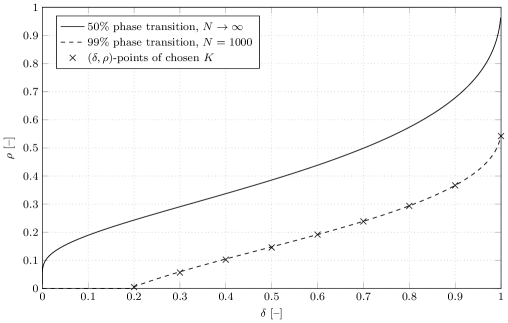
Figure 1: The theoretical Donoho-Tanner phase transition for $N\rightarrow\infty$, lower bound for $N=1000$, and points corresponding to the values of $K$ chosen for test signals.

In all simulations, we apply the proposed approach to test signals generated randomly according to the following specifications: size of $\mathbf{x}$ vector $N=1000$; number of compressed measurements $M\in\{200,300,400,500,600,700,800,900,1000\}$. The non-zero elements of $\mathbf{x}$ are i.i.d. $\sim\mathcal{N}(0,1)$; the number of non-zero elements $K$ is selected for each value of $M$. This is done by calculating the largest possible $K$ for each $M$ according to the lower bound on the $99\%$ phase transition for finite $N=1000$ by the formula given in [6, Sec. IV, Theorem 2], drawn in Fig. 1 (- - -). The resulting values are $K\in\{1,17,41,73,115,167,235,330,542\}$. The corresponding $(\delta,\rho)$-points are plotted in Fig. 1 ($\times$).

The measurement matrix $\bm{\Phi}$ has i.i.d. entries $\sim\mathcal{N}(0,\frac{1}{M})$ and we use the dictionary $\bm{\Psi}=\mathbf{I}$, so that $\mathbf{A}=\bm{\Phi}$. We repeat the experiment $T=$1000$$ times for randomly generated $\mathbf{x}$ and $\bm{\Phi}$ in each repetition and average the reconstructed signal Normalized Mean Squared Error (NMSE), $\mathcal{P}$, over all solution instances $\hat{\mathbf{x}}_{i},\ i\in\{1,\ldots,T\}$:

$$\mathcal{P}=\frac{1}{T}\sum_{i=1}^{T}\frac{\|\hat{\mathbf{x}}_{i}-\mathbf{x}_{i}\|_{2}^{2}}{\|\mathbf{x}_{i}\|_{2}^{2}}.$$ (27)

To enable assessment of the quality of the obtained results, we plot the simulated figures with error bars signifying their $99\%$ confidence intervals computed under the assumption of a Gaussian distributed mean of the NMSE, see e.g. [26, Sec. 7.3.1]. The simulations were conducted for reconstruction using regular BPDN (6) vs. our proposed approach (14) (denoted “BPDN-scale” in result plots). The numerical optimization problems were solved using the SPGL1 software package [27].

Regarding the choice of $\epsilon$, for regular BPDN (6), we chose $\epsilon$ according to (13), with $\sigma=\sqrt{\sigma^{2}_{q}}$ from (22). For our proposed approach (14), we chose $\epsilon$ according to (13), with $\sigma=\sqrt{\sigma^{2}_{r}}$ from (21). For both compared approaches, we consider $\sigma^{2}_{\bar{y}}$ known. As demonstrated in Section 4.3, $\epsilon$ could be chosen better from empirical observations to provide smaller error in the reconstruction, i.e. $\|\hat{\mathbf{x}}-\mathbf{x}\|$. We chose the values (13) as practically useful values for fairness of the evaluation of our proposed method.

As we have chosen low-rate scalar quantization to demonstrate the proposed approach to noise correlated with the measurements, we additionally performed simulations to compare the proposed method to a state-of-the-art reconstruction algorithm for 1-bit compressed sensing, Binary Iterative Hard Thresholding (BIHT) [17]. This simulation was performed by evaluating both our proposed method and BIHT over the phase space $\delta,\rho\in[0,1]$ where we discretized the range [0,1] in steps of $0.01$ for both $\delta$ and $\rho$. In each point $(\delta,\rho)$ we evaluated $\mathcal{P}$ according to (27) over $T=1000$ repetitions with different $\mathbf{x}$ and $\mathbf{A}$ in each instance. For each value $\delta\in\{0.01,0.02,\ldots,1\}$ we evaluate each of the methods from $\rho=0.01$ until $\mathcal{P}>1$. For BIHT, we generated sparse signals $\mathbf{x}$ normalized to $\|\mathbf{x}\|_{2}=1$ which is assumed by BIHT and other 1-bit compressed sensing reconstruction algorithms in general. In BIHT, estimates $\hat{\mathbf{x}}$ are re-normalised after reconstruction which is not the case in our proposed method.

All scripts required to reproduce the simulation results are openly accessible.

4 Numerical Simulation Results

In this section we present results of the numerical simulations conducted according to Section 3. Firstly, we evaluate the proposed method under artificial correlated measurement noise generated according to (7). Secondly, we evaluate the method under correlated measurement noise incurred by scalar quantization of the compressed measurements. These results are shown in Section 4.1. Furthermore, in Section 4.2 we present results of simulations comparing the proposed method to BIHT. Finally, in Section 4.3 we present results of simulations to shed light on how the choices of the parameters $\beta$ and $\epsilon$ in (16) affect the main results.

4.1 Main Results

In this section, noise variance and correlation parameters are first set equal to the corresponding parameters estimated for the Lloyd-Max quantizer used later in this section, for comparability. The parameter values for $\alpha$ are listed in Table 1.

Table 1: Correlation parameter values used in Figs. 2–4.

Equiv. quantizer resolution	$\alpha$ (Lloyd-Max)	$\alpha$ (uniform)
$1\text{\,}\mathrm{bit}\text{\,}{\mathrm{sample}}^{-1}$	$0.636\,597\,595$	$0.636\,597\,595$
$3\text{\,}\mathrm{bit}\text{\,}{\mathrm{sample}}^{-1}$	$0.965\,461\,586$	$0.962\,583\,611$
$5\text{\,}\mathrm{bit}\text{\,}{\mathrm{sample}}^{-1}$	$0.997\,494\,182$	$0.996\,506\,750$

The listed values of $\alpha$ (Lloyd-Max) are used together with $\sigma_{\mathbf{r}}^{2}$ calculated from (21) to generate correlated measurement noise according to (7). In the conducted simulations, BPDN is used to reconstruct $\hat{\mathbf{x}}_{2}$ from the compressed measurements $\mathbf{y}$. We compare the standard (correlation-unaware) reconstruction, (6), of the signal (denoted “BPDN” in Fig. 2) to the reconstruction obtained by our proposed method, (14), of scaling the reconstructed signal to account for correlation (denoted “BPDN-scale” in Fig. 2). Selected results for equivalent quantizer resolutions $1\text{\,}\mathrm{bit}\text{\,}{\mathrm{sample}}^{-1}$, $3\text{\,}\mathrm{bit}\text{\,}{\mathrm{sample}}^{-1}$, and $5\text{\,}\mathrm{bit}\text{\,}{\mathrm{sample}}^{-1}$ are shown in Fig. 2. The proposed method is observed to improve the reconstruction error $\mathcal{P}$ by $7.258\,935\,064\,559\,580\text{\,}\mathrm{dB}1.265\,073\,250\,845\,205\text{\,}\mathrm{dB}$ (for increasing $\rho$) at $1\text{\,}\mathrm{bit}\text{\,}{\mathrm{sample}}^{-1}$, $3.078\,548\,916\,636\,066\text{\,}\mathrm{dB}0.259\,461\,209\,546\,714\text{\,}\mathrm{dB}$ (for increasing $\rho$) at $3\text{\,}\mathrm{bit}\text{\,}{\mathrm{sample}}^{-1}$, and $0.863\,954\,374\,872\,776\text{\,}\mathrm{dB}0.058\,916\,440\,237\,851\text{\,}\mathrm{dB}$ (for increasing $\rho$) at $5\text{\,}\mathrm{bit}\text{\,}{\mathrm{sample}}^{-1}$.

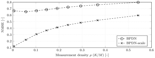
(a) Noise of var. equivalent to $1\text{\,}\mathrm{bit}\text{\,}{\mathrm{sample}}^{-1}$ quantizer.

(b) Noise of var. equivalent to $3\text{\,}\mathrm{bit}\text{\,}{\mathrm{sample}}^{-1}$ quantizer.

(c) Noise of var. equivalent to $5\text{\,}\mathrm{bit}\text{\,}{\mathrm{sample}}^{-1}$ quantizer.

Figure 2: Simulated NMSE of reconstruction using BPDN vs. relative number of measurements for parameters $\alpha$ and $\sigma_{\mathbf{r}}^{2}$ equal to corresponding values for Lloyd-Max quantizers.

The experiments for quantized measurements are conducted exactly as above, with the exception that the measurements $\mathbf{y}$ are quantized using a Lloyd-Max quantizer [23, 22]. The Lloyd-Max quantizer is designed for the Gaussian distribution of the entries of $\bar{}\mathbf{y}$ which results from the use of a measurement matrix containing i.i.d. zero-mean Gaussian entries. The correlated noise model uses the values of $\alpha$ (Lloyd-Max) for the selected quantizer resolutions listed in Table 1.

Selected results for quantizer resolutions $1\text{\,}\mathrm{bit}\text{\,}{\mathrm{sample}}^{-1}$, $3\text{\,}\mathrm{bit}\text{\,}{\mathrm{sample}}^{-1}$, and $5\text{\,}\mathrm{bit}\text{\,}{\mathrm{sample}}^{-1}$ with Lloyd-Max quantization are shown in Fig. 3. It can be observed that the reconstruction error figures $\mathcal{P}$ agree well with those simulated with artificially generated correlated noise in Fig. 2. The observed improvements by the proposed method are almost identical to those observed for artificial noise: $7.630\,424\,592\,316\,444\text{\,}\mathrm{dB}1.269\,499\,068\,230\,857\text{\,}\mathrm{dB}$ at $1\text{\,}\mathrm{bit}\text{\,}{\mathrm{sample}}^{-1}$, $3.069\,402\,388\,553\,215\text{\,}\mathrm{dB}0.260\,195\,090\,772\,186\text{\,}\mathrm{dB}$ at $3\text{\,}\mathrm{bit}\text{\,}{\mathrm{sample}}^{-1}$, and $0.795\,311\,069\,099\,512\text{\,}\mathrm{dB}0.027\,794\,290\,505\,028\text{\,}\mathrm{dB}$ at $5\text{\,}\mathrm{bit}\text{\,}{\mathrm{sample}}^{-1}$.

(a) $1\text{\,}\mathrm{bit}\text{\,}{\mathrm{sample}}^{-1}$ quantizer.

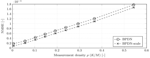
(b) $3\text{\,}\mathrm{bit}\text{\,}{\mathrm{sample}}^{-1}$ quantizer.

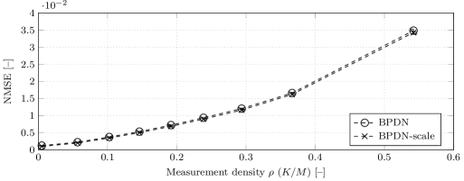
(c) $5\text{\,}\mathrm{bit}\text{\,}{\mathrm{sample}}^{-1}$ quantizer.

Figure 3: Simulated NMSE of reconstruction using BPDN vs. relative number of measurements for parameters $\alpha$ and $\sigma_{\mathbf{r}}^{2}$ equal to corresponding values for Lloyd-Max quantizers.

To evaluate our proposed approach for a more practical quantization scheme than the non-uniform Lloyd-Max quantizer, we additionally simulated results where the measurements $\mathbf{y}$ are quantized using a uniform quantizer with mid-point quantization points, optimized for minimum mean squared error (MMSE) of the quantized measurements. The uniform quantizer is designed for the Gaussian distribution of the entries of $\bar{}\mathbf{y}$. This serves to evaluate how well the proposed approach performs for a more practical quantizer type that does not theoretically obey the quantization noise model (20) due to the fact that its reconstruction points are not the centroids of the input signal’s p.d.f. in the quatizer’s input regions. The correlated noise model uses the values of $\alpha$ (uniform) from Table 1.

Selected results for quantizer resolutions $1\text{\,}\mathrm{bit}\text{\,}{\mathrm{sample}}^{-1}$, $3\text{\,}\mathrm{bit}\text{\,}{\mathrm{sample}}^{-1}$, and $5\text{\,}\mathrm{bit}\text{\,}{\mathrm{sample}}^{-1}$ with uniform quantization are shown in Fig. 4. The observed improvements by the proposed method are close to those observed for artificial noise: $7.630\,376\,055\,876\,695\text{\,}\mathrm{dB}1.269\,499\,006\,131\,298\text{\,}\mathrm{dB}$ at $1\text{\,}\mathrm{bit}\text{\,}{\mathrm{sample}}^{-1}$, $3.171\,612\,435\,612\,246\text{\,}\mathrm{dB}0.280\,326\,866\,601\,740\text{\,}\mathrm{dB}$ at $3\text{\,}\mathrm{bit}\text{\,}{\mathrm{sample}}^{-1}$, and $0.892\,202\,647\,533\,395\text{\,}\mathrm{dB}0.072\,544\,852\,438\,341\text{\,}\mathrm{dB}$ at $5\text{\,}\mathrm{bit}\text{\,}{\mathrm{sample}}^{-1}$.

(a) $1\text{\,}\mathrm{bit}\text{\,}{\mathrm{sample}}^{-1}$ quantizer.

(b) $3\text{\,}\mathrm{bit}\text{\,}{\mathrm{sample}}^{-1}$ quantizer.

(c) $5\text{\,}\mathrm{bit}\text{\,}{\mathrm{sample}}^{-1}$ quantizer.

Figure 4: Simulated NMSE of reconstruction using BPDN vs. relative number of measurements for parameters $\alpha$ and $\sigma_{\mathbf{r}}^{2}$ equal to corresponding values for uniform quantizers.

The results in Fig. 3a and 4a are identical due to the fact that the 2-level Lloyd-Max quantizer is a uniform 2-level quantizer optimized for MMSE of the quantized values. It can also be observed that the uniform quantizer for $3\text{\,}\mathrm{bit}\text{\,}{\mathrm{sample}}^{-1}5\text{\,}\mathrm{bit}\text{\,}{\mathrm{sample}}^{-1}$ results in slightly larger reconstruction error while the improvement by our proposed method is preserved.

4.2 Comparison to Binary Iterative Hard Thresholding (BIHT)

In this section, we provide results comparing our proposed method to BIHT. Results for our proposed method were computed in the same manner as for the results regarding 1-bit quantization in Section 4.1. The simulated NMSE of our proposed method and BIHT are shown in Fig. 5. The white regions of the phase space are un-tested as they lie beyond $\mathcal{P}>1$; a threshold we selected to define the region we wished to investigate. The bold contour lines mark the boundary where the NMSEs of our proposed method and BIHT are equal. As the numbered contour lines show, “BPDN-scale” exhibits lower NMSE than BIHT in the majority (upper left region) of the phase space, whereas the NMSE of BIHT is lower along the bottom of the phase space – up to around $\rho=0.1$ – and in the upper right-hand corner – towards $(\delta,\rho)=(1,1)$.

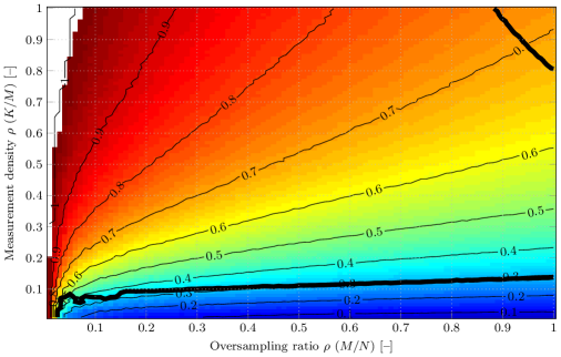
(a) Proposed method (BPDN-scale).

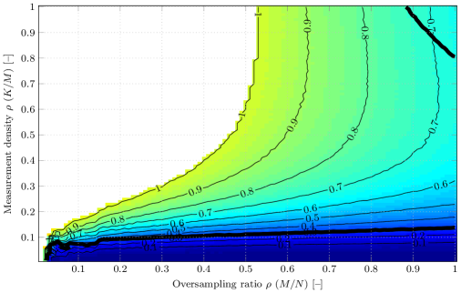
(b) BIHT.

Figure 5: Simulated NMSE of reconstruction from 1-bit quantized measurements. The numbered (—$0.1$— etc.) contour lines trace equal NMSE levels. The bold contour lines (—) mark the boundary where the NMSE levels of the proposed method and BIHT, respectively, are equal. (“Wiggly” contour lines are caused by interpolation in Matlab).

4.3 Empirical Investigation of Scaling Factors and Regularization Parameters

In order to assess the optimality of the proposed approach as described in Section 2.4, we conducted simulations for values of $\beta$ in (16) using artificial pseudo-random noise generated according to the model (20). Since the reconstruction error performance is also affected by the choice of $\epsilon$ in (16), we similarly performed the simulations over different values $\epsilon$. Preliminary simulations indicated that $\mathcal{P}$ (see (27)) evolves in a quasi-convex manner over $\beta$ and $\epsilon$. Based on this observation, we have used the Nelder-Mead simplex algorithm [28] to find the $(\beta,\epsilon)$-optimal error figures $\mathcal{P}$ for each of the points $(M,K)$ listed in Section 3. The results for all $(M,K)$ with correlated noise generated according to each of the values $\alpha$ (Lloyd-Max) in Table 1 are shown in tables  2 to  4 . The optimal regularization parameter values for ordinary BPDN are denoted $\epsilon_{1}$ – with resulting error figure $\mathcal{P}_{1}$, while the optimal scaling and regularization parameter values for the proposed method are denoted $\beta_{2}$ and $\epsilon_{2}$ – with resulting error figure $\mathcal{P}_{2}$. The error figures from our proposed method as reported in Fig. 2 are included in tables  2 to  4 as $\mathcal{P}_{\alpha}$ to facilitate comparison.

Table 2: Simulated NMSE at empirically optimal parameter values $\beta$ and $\epsilon$. Noise equivalent to $1\text{\,}\mathrm{bit}\text{\,}{\mathrm{sample}}^{-1}$ quantizer.

$(M,K)$	$\epsilon_{1}/\epsilon$	$\mathcal{P}_{1}$	$\beta_{2}/\alpha$	$\epsilon_{2}/\epsilon$	$\mathcal{P}_{2}$	$\mathcal{P}_{\alpha}$
$(200,1)$	$0.600\,000\,094$	$1.962\,764\,128\text{\cdot}{10}^{-02}$	$0.836\,230\,469$	$0.921\,484\,375$	$1.019\,192\,831\text{\cdot}{10}^{-03}$	$1.211\,786\,045\text{\cdot}{10}^{-01}$
$(300,17)$	$0.499\,999\,905$	$3.309\,425\,673\text{\cdot}{10}^{-02}$	$0.738\,657\,352$	$0.925\,879\,428$	$1.366\,921\,566\text{\cdot}{10}^{-02}$	$2.215\,994\,094\text{\cdot}{10}^{-01}$
$(400,41)$	$0.512\,988\,281$	$3.888\,425\,539\text{\cdot}{10}^{-02}$	$0.829\,915\,241$	$0.865\,297\,454$	$2.248\,581\,511\text{\cdot}{10}^{-02}$	$3.073\,345\,237\text{\cdot}{10}^{-01}$
$(500,73)$	$0.4625$	$4.271\,101\,597\text{\cdot}{10}^{-02}$	$0.772\,141\,054$	$0.931\,689\,703$	$2.889\,661\,903\text{\cdot}{10}^{-02}$	$3.657\,011\,687\text{\cdot}{10}^{-01}$
$(600,115)$	$0.512\,597\,632$	$4.472\,722\,152\text{\cdot}{10}^{-02}$	$0.792\,977\,346$	$0.901\,562\,64$	$3.445\,824\,343\text{\cdot}{10}^{-02}$	$4.112\,594\,208\text{\cdot}{10}^{-01}$
$(700,167)$	$0.474\,993\,896$	$4.605\,901\,923\text{\cdot}{10}^{-02}$	$0.882\,593\,934$	$0.843\,647\,052$	$3.801\,668\,597\text{\cdot}{10}^{-02}$	$4.501\,421\,697\text{\cdot}{10}^{-01}$
$(800,235)$	$0.499\,951\,172$	$4.783\,124\,560\text{\cdot}{10}^{-02}$	$0.997\,998\,047$	$0.739\,648\,437$	$4.172\,978\,167\text{\cdot}{10}^{-02}$	$4.846\,145\,118\text{\cdot}{10}^{-01}$
$(900,330)$	$0.456\,152\,368$	$4.895\,679\,800\text{\cdot}{10}^{-02}$	$1.034\,924\,32$	$0.730\,126\,953$	$4.527\,469\,529\text{\cdot}{10}^{-02}$	$5.212\,606\,004\text{\cdot}{10}^{-01}$
$(1000,542)$	$0.463\,378\,906$	$5.265\,562\,631\text{\cdot}{10}^{-02}$	$1.151\,389\,43$	$0.654\,899\,013$	$5.122\,387\,807\text{\cdot}{10}^{-02}$	$5.965\,638\,647\text{\cdot}{10}^{-01}$

Table 3: Simulated NMSE at empirically optimal parameter values $\beta$ and $\epsilon$. Noise equivalent to $3\text{\,}\mathrm{bit}\text{\,}{\mathrm{sample}}^{-1}$ quantizer.

$(M,K)$	$\epsilon_{1}/\epsilon$	$\mathcal{P}_{1}$	$\beta_{2}/\alpha$	$\epsilon_{2}/\epsilon$	$\mathcal{P}_{2}$	$\mathcal{P}_{\alpha}$
$(200,1)$	$0.835\,937\,5$	$5.003\,686\,966\text{\cdot}{10}^{-04}$	$0.895\,251\,465$	$1.055\,413\,82$	$3.845\,094\,096\text{\cdot}{10}^{-05}$	$7.777\,292\,419\text{\cdot}{10}^{-03}$
$(300,17)$	$0.751\,562\,5$	$1.956\,225\,894\text{\cdot}{10}^{-03}$	$0.914\,624\,023$	$0.929\,260\,254$	$8.878\,818\,358\text{\cdot}{10}^{-04}$	$1.858\,795\,845\text{\cdot}{10}^{-02}$
$(400,41)$	$0.639\,453\,125$	$3.003\,703\,742\text{\cdot}{10}^{-03}$	$0.883\,948\,517$	$0.962\,291\,336$	$1.799\,853\,026\text{\cdot}{10}^{-03}$	$3.110\,813\,475\text{\cdot}{10}^{-02}$
$(500,73)$	$0.646\,875$	$3.925\,235\,888\text{\cdot}{10}^{-03}$	$0.870\,380\,402$	$0.926\,201\,82$	$2.706\,928\,466\text{\cdot}{10}^{-03}$	$4.315\,267\,758\text{\cdot}{10}^{-02}$
$(600,115)$	$0.65$	$4.805\,505\,342\text{\cdot}{10}^{-03}$	$0.921\,708\,177$	$0.737\,433\,008$	$3.578\,545\,485\text{\cdot}{10}^{-03}$	$5.587\,304\,139\text{\cdot}{10}^{-02}$
$(700,167)$	$0.610\,937\,5$	$5.639\,735\,722\text{\cdot}{10}^{-03}$	$0.904\,189\,301$	$0.730\,999\,565$	$4.454\,644\,609\text{\cdot}{10}^{-03}$	$6.893\,618\,006\text{\cdot}{10}^{-02}$
$(800,235)$	$0.549\,609\,375$	$6.412\,675\,786\text{\cdot}{10}^{-03}$	$0.915\,832\,612$	$0.674\,575\,924$	$5.402\,928\,323\text{\cdot}{10}^{-03}$	$8.318\,545\,949\text{\cdot}{10}^{-02}$
$(900,330)$	$0.500\,195\,312$	$7.433\,060\,562\text{\cdot}{10}^{-03}$	$0.929\,301\,54$	$0.627\,553\,277$	$6.762\,944\,552\text{\cdot}{10}^{-03}$	$1.027\,183\,318\text{\cdot}{10}^{-01}$
$(1000,542)$	$0.4875$	$1.044\,461\,637\text{\cdot}{10}^{-02}$	$0.981\,768\,556$	$0.505\,537\,388$	$1.023\,121\,716\text{\cdot}{10}^{-02}$	$1.584\,817\,387\text{\cdot}{10}^{-01}$

Table 4: Simulated NMSE at empirically optimal parameter values $\beta$ and $\epsilon$. Noise equivalent to $5\text{\,}\mathrm{bit}\text{\,}{\mathrm{sample}}^{-1}$ quantizer.

$(M,K)$	$\epsilon_{1}/\epsilon$	$\mathcal{P}_{1}$	$\beta_{2}/\alpha$	$\epsilon_{2}/\epsilon$	$\mathcal{P}_{2}$	$\mathcal{P}_{\alpha}$
$(200,1)$	$0.831\,152\,344$	$1.799\,160\,130\text{\cdot}{10}^{-05}$	$0.972\,290\,802$	$1.039\,707\,18$	$2.574\,893\,847\text{\cdot}{10}^{-06}$	$5.589\,140\,078\text{\cdot}{10}^{-04}$
$(300,17)$	$0.699\,218\,75$	$1.181\,667\,478\text{\cdot}{10}^{-04}$	$0.973\,400\,879$	$0.935\,858\,154$	$6.284\,629\,468\text{\cdot}{10}^{-05}$	$1.395\,401\,644\text{\cdot}{10}^{-03}$
$(400,41)$	$0.654\,687\,5$	$2.009\,662\,307\text{\cdot}{10}^{-04}$	$0.967\,785\,645$	$0.961\,956\,787$	$1.295\,546\,072\text{\cdot}{10}^{-04}$	$2.457\,189\,756\text{\cdot}{10}^{-03}$
$(500,73)$	$0.681\,25$	$2.827\,824\,401\text{\cdot}{10}^{-04}$	$0.970\,315\,552$	$0.846\,421\,814$	$1.904\,358\,375\text{\cdot}{10}^{-04}$	$3.617\,261\,602\text{\cdot}{10}^{-03}$
$(600,115)$	$0.631\,445\,312$	$3.756\,479\,372\text{\cdot}{10}^{-04}$	$0.968\,706\,578$	$0.723\,657\,039$	$2.740\,219\,755\text{\cdot}{10}^{-04}$	$5.028\,247\,464\text{\cdot}{10}^{-03}$
$(700,167)$	$0.5$	$4.768\,401\,725\text{\cdot}{10}^{-04}$	$0.964\,893\,913$	$0.721\,007\,252$	$3.628\,962\,904\text{\cdot}{10}^{-04}$	$6.600\,790\,772\text{\cdot}{10}^{-03}$
$(800,235)$	$0.563\,281\,25$	$5.768\,559\,384\text{\cdot}{10}^{-04}$	$0.969\,677\,734$	$0.659\,985\,352$	$4.776\,633\,846\text{\cdot}{10}^{-04}$	$8.639\,184\,807\text{\cdot}{10}^{-03}$
$(900,330)$	$0.448\,437\,5$	$7.326\,732\,124\text{\cdot}{10}^{-04}$	$0.964\,321\,676$	$0.575\,938\,128$	$6.383\,322\,100\text{\cdot}{10}^{-04}$	$1.210\,708\,841\text{\cdot}{10}^{-02}$
$(1000,542)$	$0.414\,062\,5$	$1.315\,488\,557\text{\cdot}{10}^{-03}$	$0.980\,423\,737$	$0.373\,928\,452$	$1.255\,090\,752\text{\cdot}{10}^{-03}$	$2.686\,228\,056\text{\cdot}{10}^{-02}$

It was expected that $\alpha$ would be the optimal choice of $\beta$, i.e. $\beta=\alpha$. However, it turns out that the (empirically observed) optimal value of $\beta_{2}$ is typically slightly smaller than $\alpha$ with observed values $\beta_{2}\in[$0.738\,657\,352$\alpha,$0.981\,768\,556$\alpha]$, depending on $(M,K)$. An exception is seen in Table 2, where $\beta_{2}\in[$1.034\,924\,32$\alpha,$1.151\,389\,43$\alpha]$.

The optimal values of the regularization parameter $\epsilon$ are similarly found to be lower than the values given by (13). For the baseline method (6), the (empirically observed) optimal values are observed as $\epsilon_{1}\in[$0.414\,062\,5$\epsilon,$0.835\,937\,5$\epsilon]$, depending on $(M,K)$, where $\epsilon$ denotes the values given by (13) as described in Section 3. For our proposed method (14), the optimal values are generally closer to the values given by (13) with observed values $\epsilon_{2}\in[$0.373\,928\,452$\epsilon,$1.055\,413\,82$\epsilon]$, depending on $(M,K)$.

It is important to note that the demonstrated advantage of our proposed approach in Section 4.1 is not merely a result of a particularly lucky choice of $\epsilon$, as these experiments testify. The observed NMSE of our proposed method, $\mathcal{P}_{2}$, consistently outperforms the baseline approach, $\mathcal{P}_{1}$. The improvement is consistent across different correlation parameters $\alpha$ as seen in tables  2 to  4 where $\mathcal{P}_{2}$ is smaller than $\mathcal{P}_{1}$ by $12.8461\text{\,}\mathrm{dB}11.1438\text{\,}\mathrm{dB}8.4431\text{\,}\mathrm{dB}$ in tables  2 to  4 , respectively, for $(M,K)=(200,1)$. At the other extreme of $(M,K)=(1000,542)$, $\mathcal{P}_{2}$ is smaller than $\mathcal{P}_{1}$ by $0.1197\text{\,}\mathrm{dB}0.0897\text{\,}\mathrm{dB}0.2041\text{\,}\mathrm{dB}$, respectively. Additionally, the observed NMSEs $\mathcal{P}_{2}$ are generally around an order of magnitude lower than $\mathcal{P}_{\alpha}$ arising from our proposed choices of $\beta=\alpha$ and $\epsilon$ according to (13). However, note that $\beta_{2}$ and $\epsilon_{2}$ optimized through simulations are not practically useful.

5 Discussion

As seen from the experimental results in Section 4.3, the correlation parameter $\alpha$ from (7) may in fact not be the optimal choice of scaling parameter, as expressed by $\beta$ in (16). The generally smaller values found in Section 4.3 to be optimal for BPDN reconstruction according to (16) can be explained by the fact that they scale the estimate $\hat{\mathbf{x}}_{\beta}$ larger. It is well-known in the literature that the $\ell_{1}$-norm minimization approach represented by, e.g., (6) tends to penalize larger coefficients of $\mathbf{x}$ more than smaller coefficients [29], thus estimating the former relatively too small. Therefore, it is possible to choose a scaling parameter $\beta<\alpha$ in (16) that improves the estimate $\hat{\mathbf{x}}_{\beta}$, i.e. yields smaller $\|\hat{\mathbf{x}}_{\beta}-\mathbf{x}\|$ compared to $\|\hat{\mathbf{x}}_{\alpha}-\mathbf{x}\|$. At this time, we cannot quantify the optimal $\beta$ analytically and it depends on the indeterminacy and/or measurement density of the performed compressed sensing.

Regarding the comparison of the proposed method to BIHT, the two methods require two different kinds of prior information. BIHT requires knowing that the sparse vector $\mathbf{x}$ is unit-norm: $\|\mathbf{x}\|_{2}=1$. Our proposed method requires knowing the variance of the unquantized measurements $\bar{y}$ – the elements of $\bar{}\mathbf{y}$. It may depend on the specific application which quantity is more realistic to know about the signal. At least, the variance assumed known in our proposed method does not require any knowledge (such as norm) of the sparse representation $\mathbf{x}$ of the observed signal.

6 Conclusion

We proposed a simple technique to model correlation between measurements and an additive noise in compressed sensing signal reconstruction. The technique is based on a linear model of the correlation between the measurements and noise. It consists of scaling signals reconstructed by a well-known $\ell_{1}$-norm convex optimization method according to the model and comes at negligible computational cost. We provided practical expressions for computing the scaling parameter and the reconstruction regularization parameter.

We performed numerical simulations to demonstrate the obtainable reconstruction error improvement by the proposed method compared to ordinary $\ell_{1}$-norm convex optimization reconstruction for noise generated according to the model. We further demonstrated as an example that the model applies well to low-rate scalar quantization of the measurements; both Lloyd-Max quantization that complies accurately with the correlation model, as well as the more practical uniform quantization. For example, simulations indicated that the proposed method offers improvements on the order of $1\text{\,}\mathrm{dB}7\text{\,}\mathrm{dB}$ for $1\text{\,}\mathrm{bit}\text{\,}{\mathrm{sample}}^{-1}$ quantization, depending on the indeterminacy of the performed compressed sensing.

We compared the proposed approach to a state-of-the-art reconstruction method, Binary Iterative Hard Thresholding (BIHT), for the special case of $1\text{\,}\mathrm{bit}\text{\,}{\mathrm{sample}}^{-1}$ quantization. This comparison showed that the proposed approach reconstructs signals with smaller error than BIHT when the signals contain more non-zero elements than an approximate fraction of $0.1$ of the number of measurements. This indicated that the proposed method is able to reconstruct less sparse signals from 1-bit quantized measurements than BIHT is capable of.

We conducted numerical simulations to evaluate the validity of our results which confirmed that the improvements offered by the proposed method are not merely a coincidental result of the suggested practical choices of scaling and optimization regularization parameters. These results further indicated that the proposed method is robust to the choice of scaling and optimization regularization parameter in the sense that a suboptimal choice still leads to considerable improvements over the ordinary convex optimization reconstruction method.

References

References

- [1] D. Donoho, Compressed sensing, IEEE Trans. Inf. Theory 52 (4) (2006) 1289–1306. doi:10.1109/TIT.2006.871582.
- [2] E. J. Candès, J. Romberg, T. Tao, Robust uncertainty principles: exact signal reconstruction from highly incomplete frequency information, IEEE Trans. Inf. Theory 52 (2) (2006) 489–509. doi:10.1109/TIT.2005.862083.
- [3] E. J. Candès, Compressive sampling, in: Proceedings of the International Congress of Mathematicians, Vol. 3, 2006, pp. 1433–1452.
- [4] E. J. Candès, Y. C. Eldar, D. Needell, P. Randall, Compressed sensing with coherent and redundant dictionaries, Applied and Computational Harmonic Analysis 31 (1) (2011) 59–73. doi:10.1016/j.acha.2010.10.002.
- [5] E. J. Candès, T. Tao, Decoding by linear programming, IEEE Trans. Inf. Theory 51 (12) (2005) 4203–4215. doi:10.1109/TIT.2005.858979.
- [6] D. Donoho, J. Tanner, Precise undersampling theorems, Proc. IEEE 98 (6) (2010) 913–924. doi:10.1109/JPROC.2010.2045630.
- [7] E. J. Candès, T. Tao, Near-optimal signal recovery from random projections: Universal encoding strategies?, IEEE Trans. Inf. Theory 52 (12) (2006) 5406–5425. doi:10.1109/TIT.2006.885507.
- [8] R. Tibshirani, Regression shrinkage and selection via the lasso, Journal of the Royal Statistical Society. Series B (Methodological) 58 (1) (1996) 267–288.
- [9] S. S. Chen, D. L. Donoho, M. A. Saunders, Atomic decomposition by basis pursuit, SIAM J. Sci. Comput. 20 (1) (1998) 33–61. doi:10.1137/S1064827596304010.
- [10] E. Candes, T. Tao, The Dantzig selector: Statistical estimation when p is much larger than n, Annals of Statistics 35 (6) (2007) 2313–2351. doi:10.1214/009053606000001523.
- [11] T. Blumensath, M. Davies, Normalized iterative hard thresholding: Guaranteed stability and performance, IEEE J. Sel. Topics Signal Process. 4 (2) (2010) 298–309. doi:10.1109/JSTSP.2010.2042411.
- [12] W. Dai, O. Milenkovic, Subspace pursuit for compressive sensing signal reconstruction, IEEE Trans. Inf. Theory 55 (5) (2009) 2230–2249. doi:10.1109/TIT.2009.2016006.
- [13] D. Needell, J. A. Tropp, CoSaMP: Iterative signal recovery from incomplete and inaccurate samples, Applied and Computational Harmonic Analysis 26 (3) (2009) 301–321. doi:10.1016/j.acha.2008.07.002.
- [14] A. Maleki, D. Donoho, Optimally tuned iterative reconstruction algorithms for compressed sensing, IEEE J. Sel. Topics Signal Process. 4 (2) (2010) 330–341. doi:10.1109/JSTSP.2009.2039176.
- [15] M. Raginsky, R. Willett, Z. Harmany, R. Marcia, Compressed sensing performance bounds under poisson noise, Signal Processing, IEEE Transactions on 58 (8) (2010) 3990–4002. doi:10.1109/TSP.2010.2049997.
- [16] L. Jacques, D. Hammond, J. Fadili, Dequantizing compressed sensing: When oversampling and non-gaussian constraints combine, Information Theory, IEEE Transactions on 57 (1) (2011) 559–571. doi:10.1109/TIT.2010.2093310.
- [17] L. Jacques, J. Laska, P. Boufounos, R. Baraniuk, Robust 1-bit compressive sensing via binary stable embeddings of sparse vectors, IEEE Trans. Inf. Theory 59 (4) (2013) 2082–2102. doi:10.1109/TIT.2012.2234823.
- [18] P. C. Hansen, Rank-Deficient and Discrete Ill-Posed Problems: Numerical Aspects of Linear Inversion (Monographs on Mathematical Modeling and Computation), Society for Industrial Mathematics, Philadelphia, 1987.
- [19] S. Becker, J. Bobin, E. J. Candes, NESTA: A fast and accurate first-order method for sparse recovery, SIAM Journal on Imaging Sciences 4 (1) (2011) 1–39. doi:10.1137/090756855.
- [20] M. Elad, Sparse and Redundant Representations: From Theory to Applications in Signal and Image Processing, Springer, New York, 2010. doi:10.1007/978-1-4419-7011-4.
- [21] N. S. Jayant, P. Noll, Digital Coding of Waveforms - Principles and Applications to Speech and Video, Prentice Hall, Englewood Cliffs, New Jersey, 1984.
- [22] S. Lloyd, Least squares quantization in PCM, IEEE Trans. Inf. Theory 28 (2) (1982) 129–137. doi:10.1109/TIT.1982.1056489.
- [23] J. Max, Quantizing for minimum distortion, IEEE Trans. Inf. Theory 6 (1) (1960) 7–12. doi:10.1109/TIT.1960.1057548.
- [24] P. H. Westerink, J. Biemond, D. E. Boekee, Scalar quantization error analysis for image subband coding using qmfs, IEEE Trans. Signal Process. 40 (2) (1992) 421–428. doi:10.1109/78.124952.
- [25] D. Donoho, A. Maleki, A. Montanari, The noise-sensitivity phase transition in compressed sensing, IEEE Trans. Inf. Theory 57 (10) (2011) 6920–6941. doi:10.1109/TIT.2011.2165823.
- [26] S. M. Ross, Introduction to Probability and Statistics for Engineers and Scientists, 2nd Edition, Academic Press, San Diego, 2000.
- [27] E. van den Berg, M. P. Friedlander, Probing the Pareto frontier for basis pursuit solutions, SIAM J. Sci. Comput. 31 (2) (2008) 890–912. doi:10.1137/080714488.
- [28] J. A. Nelder, R. Mead, A simplex method for function minimization, The Computer Journal 7 (4) (1965) 308–313. doi:10.1093/comjnl/7.4.308.
- [29] E. Candès, M. Wakin, S. Boyd, Enhancing sparsity by reweighted minimization, Journal of Fourier Analysis and Applications 14 (5) (2008) 877–905. doi:10.1007/s00041-008-9045-x.