Applying Strategic Multiagent Planning to Real-World Travel Sharing Problems

Abstract

Travel sharing, i.e., the problem of finding parts of routes which can be shared by several travellers with different points of departure and destinations, is a complex multiagent problem that requires taking into account individual agents’ preferences to come up with mutually acceptable joint plans. In this paper, we apply state-of-the-art planning techniques to real-world public transportation data to evaluate the feasibility of multiagent planning techniques in this domain. The potential of improving travel sharing technology has great application value due to its ability to reduce the environmental impact of travelling while providing benefits to travellers at the same time.

We propose a three-phase algorithm that utilises performant single-agent planners to find individual plans in a simplified domain first and then merges them using a best-response planner which ensures resulting solutions are individually rational. Finally, it maps the resulting plan onto the full temporal planning domain to schedule actual journeys.

The evaluation of our algorithm on real-world, multi-modal public transportation data for the United Kingdom shows linear scalability both in the scenario size and in the number of agents, where trade-offs have to be made between total cost improvement, the percentage of feasible timetables identified for journeys, and the prolongation of these journeys. Our system constitutes the first implementation of strategic multiagent planning algorithms in large-scale domains and provides insights into the engineering process of translating general domain-independent multiagent planning algorithms to real-world applications.

1 Introduction

Travelling is an important and frequent activity, yet people willing to travel have to face problems with rising fuel prices, carbon footprint and traffic jams. These problems can be ameliorated by travel sharing, i.e., groups of people travel together in one vehicle for parts of the journey. Participants in such schemes can benefit from travel sharing in several ways: sharing parts of a journey may reduce cost (e.g., through group tickets), carbon footprint (e.g., when sharing a private car, or through better capacity utilisation of public means of transport), and travellers can enjoy the company of others on a long journey. In more advanced scenarios one could even imagine this being combined with working together while travelling, holding meetings on the road, etc.

Today, there exist various commercial online services for car, bike, and walk sharing as well as services which assist users in negotiating shared journeys, and, of course, plenty of travel planning services that automate individual travel planning for one or several means of transport. On the research side, there is previous work that deals with the ridesharing and car-pooling problem [1, 8, 14]. However, no work has been done that attempts to compute joint travel plans based on public transportation timetable data and geographical stop locations, let alone in a way that takes into account the strategic nature of the problem, which comes about through the different (and potentially conflicting) preferences of individuals who might be able to benefit from travelling together. From the point of view of (multiagent) planning, this presents itself as a very complex application scenario: Firstly, even if one restricted oneself to centralised (non-strategic) planning, the domain is huge – public transportation data for the UK alone currently involves $240,590$ timetable connections for trains and coaches (even excluding local city buses), which would have to be translated to a quarter of a million planning actions, at least in a naive formalisation of the domain. Secondly, planning for multiple self-interested agents that are willing to cooperate only if it is beneficial for them is known to be exponentially harder than planning for each agent individually [2]. Yet any automated service that proposes joint journeys would have to guarantee such strategic properties in order to be acceptable for human users (who could then even leave it to the service to negotiate trips on their behalf).

In this paper, we present an implementation of best-response planning (BRP) [13] within a three-phase algorithm that is capable of solving strategic travel sharing problems for several agents based on real-world transportation data. Based on a simplified version of the domain that ignores timetabling information, the algorithm first builds individual travel plans using state-of-the-art single-agent planners that are available off the shelf. It then merges these individual plans and computes a multiagent plan that is a Nash equilibrium and guarantees individual rationality of solutions, as well as stability in the sense that no single agent has an incentive to deviate from the joint travel route. This is done using BRP as the underlying planner, as it is the only available planner that can solve strategic multiagent planning problems of such scale, and is proven to converge in domains that comply with certain assumptions, as is the case for our travel sharing domain. In a third and final step, the resulting multiagent plan is mapped onto the full temporal planning domain to schedule actual journeys. This scheduling task is not guaranteed to always find a feasible solution, as the previous simplification ignores a potential lack of suitable connections. However, we show through an extensive empirical evaluation that our method finds useful solutions in a large number of cases despite its theoretical incompleteness.

The contribution of our work is threefold: Firstly, we show that current multiagent planning technology can be used in important planning domains such as travel sharing by presenting its application to a practical problem that cannot be solved with other existing techniques. In the process, we describe the engineering steps that are necessary to deal with the challenges of real-world large-scale data and propose suitable solutions. Secondly, we present an algorithm that combines different techniques in a practically-oriented way, and which is largely based on domain-independent off-the-shelf heuristic problem solvers. In fact, only data preprocessing and timetable mapping use domain-specific knowledge, and much of the process of incorporating this knowledge could be replicated for similar other domains (such as logistics, manufacturing, and network communications). Finally, we provide a potential solution to the hard computational problem of travel sharing that could be exploited for automating important tasks in a future real-world application to the benefits of users, who normally have to plan such routes manually and would be overwhelmed by the choices in a domain full of different transportation options which is inhabited by many potential co-travellers.

We start off by describing the problem domain in section 2 and specifying the planning problem formally in section 3, following the model used in [13]. Section 4 introduces our three-phase algorithm for strategic planning in travel sharing domains and we present an extensive experimental evaluation of the algorithm in section 5. Section 6 presents a discussion of our results and section 7 concludes.

2 The travel sharing domain

The real-world travel domain used in this paper is based on the public transport network in the United Kingdom, a very large and complex domain which contains $4,055$ railway and coach stops supplemented by timetable information. An agent representing a passenger is able to use different means of transport during its journey: walking, trains, and coaches. The aim of each agent is to get from its starting location to its final destination at the lowest possible cost, where the cost of the journey is based on the duration and the price of the journey. Since we assume that all agents are travelling on the same day and that all journeys must be completed within 24 hours, in what follows below we consider only travel data for Tuesdays (this is an arbitrary choice that could be changed without any problem). For the purposes of this paper, we will make the assumption that sharing a part of a journey with other agents is cheaper than travelling alone. While this may not currently hold in many public transportation systems, defining hypothetical cost functions that reflect this would help assess the potential benefit of introducing such pricing schemes.

2.1 Source data

The travel sharing domain uses the National Public Transport Data Repository (NPTDR) which is publicly available from the Department for Transport of the British Government. It contains a snapshot of route and timetable data that has been gathered in the first or second complete week of October since 2004. For the evaluation of the algorithm in section 5, we used data from 2010, which is provided in TransXChange XML.

National Public Transport Access Nodes (NaPTAN) is a UK national system for uniquely identifying all the points of access to public transport. Every point of access (bus stop, rail station, etc.) is identified by an ATCO code, e.g., 9100HAYMRKT for Haymarket Rail Station in Edinburgh. Each stop in NaPTAN XML data is also supplemented by common name, latitude, longitude, address and other pieces of information. This data also contains information about how the stops are grouped together (e.g., several bus bays that are located at the same bus station).

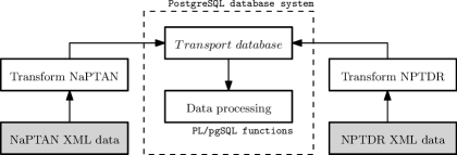
Figure 1: Overview of the data transformation and processing

To be able to use this domain data with modern AI planning systems, it has to be converted to the Planning Domain Definition Language (PDDL). We transformed the data in three subsequent stages, cf. Figure 1. First, we transformed the NPTDR and NaPTAN XML data to a spatially-enabled PostgreSQL database. Second, we automatically processed and optimised the data in the database. The data processing by SQL functions in the procedural PL/pgSQL language included the following steps: merging bus bays at bus stations and parts of train stations, introducing walking connections to enable multi-modal journeys, and eliminating duplicates from the timetable. Finally, we created a script for generating PDDL specifications based on the data in the database. More details about the data processing and PDDL specifications can be found in [11].

Figure 2: An example of the relaxed domain (e.g., it takes 50 minutes to travel from the stop $\boldsymbol{A}$ to $\boldsymbol{B}$)

2.2 Planning domain definitions

Since the full travel planning domain is too large for any current state-of-the-art planner to deal with, we distinguish the full domain from a relaxed domain, which we will use to come up with an initial plan before mapping it to the full timetable information in our algorithm below.

The relaxed domain is a single-agent planning domain represented as a directed graph where the nodes are the stops and the edges are the connections provided by a service. The graph must be directed because there exist stops that are used in one direction only. There is an edge from $A$ to $B$ if there is at least one connection from $A$ to $B$ in the timetable. The cost of this edge is the minimal time needed for travelling from $A$ to $B$. A plan $P_{i}$ found in the relaxed domain for the agent $i$ is a sequence of connections to travel from its origin to its destination. The relaxed domain does not contain any information about the traveller’s departure time. This could be problematic in a scenario where people are travelling at different times of day. This issue could be solved by clustering of user requests, cf. chapter 7.

A small example of the relaxed domain is shown in Figure 2. An example plan for an agent travelling from $C$ to $F$ is $P_{1}=\langle C\rightarrow D,D\rightarrow E,E\rightarrow F\rangle$. To illustrate the difference between the relaxed domain and the full timetable, there are $8,688$ connections in the relaxed domain for trains and coaches in the UK compared to $240,590$ timetable connections.

Direct trains that do not stop at every stop are filtered out from the relaxed domain for the following reason: Assume that in Figure 2, there is only one agent travelling from $C$ to $F$ and that its plan in the relaxed domain is to use a direct train from $C$ to $F$. In this case, it is only possible to match its plan to direct train connections from $C$ to $F$, and not to trains that stop at $C$, $D$, $E$, and $F$. Therefore, the agent’s plan cannot be matched against all possible trains between $C$ and $F$ which is problematic especially in the case where the majority of trains stop at every stop and only a few trains are direct. On the other hand, it is possible to match a plan with a train stopping in every stop to a direct train, as it is explained later in section 4.3.

The full domain is a multiagent planning domain based on the joint plan $P$. Assume that there are $N$ agents in the full domain (each agent $i$ has the plan $P_{i}$ from the relaxed domain). Then, the joint plan $P$ is a merge of single-agent plans defined by formula

$$P=\bigcup_{i=1}^{N}P_{i}$$

where we interpret $\bigcup$ as the union of graphs that would result from interpreting each plan as a set of edges connecting stops. More specifically, given a set of single-agent plans, the plan merging operator $\bigcup$ computes its result in three steps: First, it transforms every single-agent plan $P_{i}$ to a directed graph $G_{i}$ where the nodes are the stops from the single-agent plan $P_{i}$ and the edges represent the actions of $P_{i}$ (for instance, a plan $P_{1}=\langle C\rightarrow D,D\rightarrow E,E\rightarrow F\rangle$ is transformed to a directed graph $G_{1}=\{C\rightarrow D\rightarrow E\rightarrow F\}$). Second, it performs a graph union operation over the directed graphs $G_{i}$ and labels every edge in the joint plan with the numbers of agents that are using the edge (we don’t introduce any formal notation for these labels here, and simply slightly abuse the standard notation of sets of edges to describe the resulting graph).

As an example, the joint plan for agent 1 travelling from $C$ to $F$ and sharing a journey from $D$ to $E$ with agent 2 would be computed as

$$\langle C\rightarrow D,D\rightarrow E,E\rightarrow F\rangle\>\cup\>\langle D\rightarrow E\rangle=\\ \{C\xrightarrow{(1)}D\xrightarrow{(1,2)}E\xrightarrow{(1)}F\}$$

With this, the full domain is represented as a directed multigraph where the nodes are the stops that are present in the joint plan of the relaxed domain. Edges of the multigraph are the service journeys from the timetable. Every service is identified by a unique service name and is assigned a departure time from each stop and the duration of its journey between two stops. In the example of the full domain in Figure 3, the agents can travel using some subset of five different services S1 to S5. In order to travel from $C$ to $D$ using service S1, an agent must be present at stop $C$ before its departure.

Figure 3: An example of the full domain with stops $\boldsymbol{C}$, $\boldsymbol{D}$, $\boldsymbol{E}$ and $\boldsymbol{F}$ for the joint plan $\boldsymbol{P}\boldsymbol{=}\boldsymbol{\{}\boldsymbol{C}\xrightarrow{(1)}\boldsymbol{D}\xrightarrow{(1,2)}\boldsymbol{E}\xrightarrow{(1)}\boldsymbol{F}\boldsymbol{\}}$

3 The planning problem

Automated planning technology [9] has developed a variety of scalable heuristic algorithms for tackling hard planning problems, where plans, i.e., sequences of actions that achieve a given goal from a given initial state, are calculated by domain-independent problem solvers. To model the travel sharing problem, we use a multiagent planning formalism which is based on MA-STRIPS [2] and coalition-planning games [3]. States are represented by sets of ground fluents, actions are tuples $a=\langle\mathit{pre}(a),\mathit{eff}(a)\rangle$. After the execution of action $a$, positive fluents $p$ from $\mathit{eff}(a)$ are added to the state and negative fluents $\neg p$ are deleted from the state. Each agent has individual goals and actions with associated costs. There is no extra reward for achieving the goal, the total utility received by an agent is simply the inverse of the cost incurred by the plan executed to achieve the goal.

More formally, following the notation of [13], a multiagent planning problem (MAP) is a tuple

$$\Pi=\langle N,F,I,\{G_{i}\}_{i=1}^{n},\{A_{i}\}_{i=1}^{n},\Psi,\{c_{i}\}_{i=1}^{n}\rangle$$

where

• $N=\{1,\ldots,n\}$ is the set of agents,

• $F$ is the set of fluents,

• $I\subseteq F$ is the initial state,

• $G_{i}\subseteq F$ is agent $i$’s goal,

• $A_{i}$ is agent $i$’s action set,

• $\Psi:A\rightarrow\{0,1\}$ is an admissibility function,

• $c_{i}:\times_{i=1}^{n}A_{i}\rightarrow\mathbb{R}$ is the cost function of agent $i$.

$A=A_{1}\times\ldots\times A_{n}$ is the joint action set assuming a concurrent, synchronous execution model, and $G=\wedge_{i}G_{i}$ is the conjunction of all agents’ individual goals. A MAP typically imposes concurrency constraints regarding actions that cannot or have to be performed concurrently by different agents to succeed which the authors of [13] encode using an admissibility function $\Psi$, with $\Psi(a)=1$ if the joint action $a$ is executable, and $\Psi(a)=0$ otherwise.

A plan $\pi=\langle a^{1},\ldots,a^{k}\rangle$ is a sequence of joint actions $a^{j}\in A$ such that $a^{1}$ is applicable in the initial state $I$ (i.e., $\mathit{pre}(a^{1})\subseteq I$), and $a^{j}$ is applicable following the application of $a^{1},\ldots,$ $a^{j-1}$. We say that $\pi$ solves the MAP $\Pi$ if the goal state $G$ is satisfied following the application of all actions in $\pi$ in sequence. The cost of a plan $\pi$ to agent $i$ is given by $C_{i}(\pi)=\sum_{j=1}^{k}c_{i}(a^{j})$. Each agent’s contribution to a plan $\pi$ is denoted by $\pi_{i}$ (a sequence of $a_{i}\in A_{i}$).

3.1 Best-response planning

The best-response planning (BRP) algorithm proposed in [13] is an algorithm which, given a solution $\pi^{k}$ to a MAP $\Pi$, finds a solution $\pi^{k+1}$ to a transformed planning problem $\Pi_{i}$ with minimum cost $C_{i}(\pi^{k+1})$ among all possible solutions:

$$\pi^{k+1}=\arg\min\{C_{i}(\pi)|\pi\textrm{ identical to }\pi^{k}\textrm{ for all }j\neq i\}$$

The transformed planning problem $\Pi_{i}$ is obtained by rewriting the original problem $\Pi$ so that all other agents’ actions are fixed, and agent $i$ can only choose its own actions in such a way that all other agents still can perform their original actions. Since $\Pi_{i}$ is a single-agent planning problem, any cost-optimal planner can be used as a best-response planner.

In [13], the authors show how for a class of congestion planning problems, where all fluents are private, the transformation they propose allows the algorithm to converge to a Nash equilibrium if agents iteratively perform best-response steps using an optimal planner. This requires that every agent can perform its actions without requiring another agent, and hence can achieve its goal in principle on its own, and conversely, that no agent can invalidate other agents’ plans. Assuming infinite capacity of vehicles, the relaxed domain is an instance of a congestion planning problem.

The BRP planner works in two phases: In the first phase, an initial plan for each agent is computed (e.g., each agent plans independently or a centralised multi-agent planner is used). In the second phase, the planner solves simpler best-response planning problems from the point of view of each individual agent. The goal of the planner in a BRP problem is to minimise the cost of an agent’s plan without changing the plans of others. Consequently, it optimises a plan of each agent with respect to the current joint plan.

This approach has several advantages. It supports full concurrency of actions and the BRP phase avoids the exponential blowup in the action space resulting in much improved scalability. For the class of potential games [16], it guarantees to converge to a Nash equilibrium. On the other hand, it does not guarantee the optimality of a solution, i.e., the quality of the equilibrium in terms of overall efficiency is not guaranteed (it depends on which initial plan the agents start off with). However, experiments have proven that it can be successfully used for improving general multiagent plans [13]. Such non-strategic plans can be computed using a centralised multiagent planner, i.e., a single-agent planner (for instance Metric-FF [10]) which tries to optimise the value of the joint cost function (in our case the sum of the values of the cost functions of agents in the environment) while trying to achieve all agents’ goals. Centralised multiagent planners have no notion of self-interested agents, i.e., they ignore the individual preferences of agents.

4 A three-phase strategic travel sharing algorithm

The main problem when planning for multiple agents with a centralised multiagent planner is the exponential blowup in the action space which is caused by using concurrent, independent actions [13]. Using a naive PDDL translation has proven that a direct application of a centralised multiagent planner to this problem does not scale well. For example, a simple scenario with two agents, ferries to Orkney Islands and trains in the area between Edinburgh and Aberdeen resulted in a one-day computation time.

As mentioned above, we tackle the complexity of the domain by breaking down the planning process into different phases that avoid dealing with the full fine-grained timetable data from the outset. Our algorithm, which is shown in Figure 4, is designed to work in three phases.

4.1 The initial phase

First, in the initial phase, an initial journey is found for each agent using the relaxed domain. A journey for each agent is calculated independently of other agents in the scenario using a single-agent planner. As a result, each agent is assigned a single-agent plan which will be further optimised in the next phase. This approach makes sense in our domain because the agents do not need each other to achieve their goals and they cannot invalidate each other’s plans.

Input

• a relaxed domain

• a set of $N$ agents $A=\{a_{1},\dots,a_{N}\}$

• an origin and a destination for each agent

1. The initial phase

For $i=1,\dots,N$ do

  Find an initial journey for agent $a_{i}$ using
a single-agent planner.

2. The BR phase

Do until no change in the cost of the joint plan

For $i=1,\dots,N$ do

1. Create a simpler best-response planning (BRP)
   problem from the point of view of agent $a_{i}$.

2. Minimise the cost of $a_{i}$’s plan without changing
   the plans of others.

End

3. The timetabling phase

Identify independent groups of agents $G=\{g_{1},\dots,g_{M}\}$.

For $i=1,\dots,M$ do

1. Find the relevant timetable for group $g_{i}$.

2. Match the joint plan of $g_{i}$ to timetable using a temporal single-agent planner in the full domain with the relevant timetable.

End

Figure 4: Three-phase algorithm for finding shared journeys for agents

4.2 The BR phase

Second, in the BR phase (best-response phase), which is also based on the relaxed domain, the algorithm uses the BRP algorithm as described above. It iteratively creates and solves simpler best-response planning problems from the point of view of each individual agent. In the case of the relaxed domain, the BRP problem looks almost the same as a problem of finding a single-agent initial journey. The difference is that the cost of travelling is smaller when an agent uses a connection which is used by one or more other agents, as will be explained below, cf. equation (1).

Iterations over agents continue until there is no change in the cost of the joint plan between two successive iterations. This means that the joint plan cannot be further improved using the best-response approach. The output of the BR phase is the joint plan $P$ in the relaxed domain (defined in section 2.2) that specifies which connections the agents use for their journeys and which segments of their journeys are shared. The joint plan $P$ will be matched to the timetable in the final phase of the algorithm.

4.3 The timetabling phase

In the final timetabling phase, the optimised shared journeys are matched against timetables using a temporal single-agent planner which assumes the full domain. For this, as a first step, independent groups of agents with respect to journey sharing are identified. An independent group of agents is defined as an edge disjoint subgraph of the joint plan $P$. This means that actions of independent groups do not affect each other so it is possible to find a timetable for each independent group separately.

Then, for every independent group, parts of the group journey are identified. A part of the group journey is defined as a maximal continuous segment of the group journey which is performed by the same set of agents. As an example, there is a group of two agents that share a segment of their journeys in Figure 5: Agent 1 travels from $A$ to $G$ while agent 2 travels from $B$ to $H$. Their group journey has five parts, with the shared part (part 3) of their journey occurring between stops $C$ and $F$.

Figure 5: Parts of the group journey of two agents

Figure 6: The full domain with services from the relevant timetable. There are five different trains T1 to T5, and train T1 is a direct train.

Table 1: Parameters of the testing scenarios

Scenario code	S1	S2	S3	S4	S5
Number of stops	344	721	$1\>044$	$1\>670$	$2\>176$
Relaxed domain connections	744	$1\>520$	$2\>275$	$4\>001$	$4\>794$
Timetabled connections	$23\>994$	$26\>702$	$68\>597$	$72\>937$	$203\>590$
Means of transport	trains	trains, coaches	trains	trains, coaches	trains

In order to use both direct and stopping trains when the group journey is matched to the timetable, the relevant timetable for a group journey is composed in the following way: for every part of the group journey, return all timetable services in the direction of agents’ journeys which connect the stops in that part. An example of the relevant timetable for a group of agents from the previous example is shown in Figure 6. Now, the agents can travel using the direct train T1 or using train T2 with intermediate stops.

The relevant timetable for the group journey is used with the aim to cut down the amount of data that will be given to a temporal single-agent planner. For instance, there are $23\,994$ timetabled connections in Scotland. For an example journey of two agents, there are only 885 services in the relevant timetable which is approximately 4 % of the data. As a result, the temporal single-agent planner gets only the necessary amount of data as input, to prevent the time-consuming exploration of irrelevant regions of the state space.

4.4 Cost functions

The timetable data used in this paper (cf. section 2.1) contains neither information about ticket prices nor distances between adjacent stops, only durations of journeys from one stop to another. This significantly restricts the design of cost functions used for the planning problems. Therefore, the cost functions used in the three phases of the algorithm are based solely on the duration of journeys.

In the initial phase, every agent tries to get to its destination in the shortest possible time. The cost of travelling between adjacent stops $A$ and $B$ is simply the duration of the journey between stops $A$ and $B$. In the BR phase, we design the cost function in such a way that it favours shared journeys. The cost $c_{i,n}$ for agent $i$ travelling from $A$ to $B$ in a group of $n$ agents is then defined by equation (1):

$$c_{i,n}=\left(\frac{1}{n}\,0.8+0.2\right)c_{i}$$ (1)

where $c_{i}$ is the individual cost of the single action to $i$ when travelling alone. In our experiments below, we take this to be equal to the duration of the trip from $A$ to $B$.

This is designed to approximately model the discount for the passengers if they buy a group ticket: The more agents travel together, the cheaper the shared (leg of a) journey becomes for each agent. Also, an agent cannot travel any cheaper than 20 % of the single-agent cost. In reality, pricing for group tickets could vary, and while our experimental results assume this specific setup, the actual price calculation could be easily replaced by any alternative model.

In the timetabling phase, every agent in a group of agents tries to spend the shortest possible time on its journey. When matching the plan to the timetable, the temporal planner tries to minimise the sum of durations of agents’ journeys including waiting times between services.

5 Evaluation

We have evaluated our algorithm on public transportation data for the United Kingdom, using various off-the-shelf planners for the three phases described above, and a number of different scenarios. These are described together with the results obtained from extensive experiments below.

5.1 Planners

All three single-agent planners used for the evaluation were taken from recent International Planning Competitions (IPC) from 2008 and 2011. We use LAMA [18] in the initial and the BR phase, a sequential satisficing (as opposed to cost-optimal) planner which searches for any plan that solves a given problem and does not guarantee optimality of the plans computed. LAMA is a propositional planning system based on heuristic state-space search. Its core feature is the usage of landmarks [17], i.e., propositions that must be true in every solution of a planning problem.

SGPlan₆ [12] and POPF2 [7] are temporal satisficing planners used in the timetabling phase. Such temporal planners take the duration of actions into account and try to minimise makespan (i.e., total duration) of a plan but do not guarantee optimality. The two planners use different search strategies and usually produce different results. This allows us to run them in sequence on every problem and to pick the plan with the shortest duration. It is not strictly necessary to run both planners, one could save computation effort by trusting one of them.

SGPlan₆ consists of three inter-related steps: parallel decomposition, constraint resolution and subproblem solution [4, 10, 15, 19]. POPF2 is a temporal forward-chaining partial-order planner with a specific extended grounded search strategy described in [5, 6]. It is not known beforehand which of the two planners will return a better plan on a particular problem instance.

5.2 Scenarios

To test the performance of our algorithm, we generated five different scenarios of increasing complexity, whose parameters are shown in Table 1. They are based on different regions of the United Kingdom (Scotland for S1 and S2, central UK for S3 and S4, central and southern UK for S5). Each scenario assumes trains or trains and coaches as available means of transportation.

In order to observe the behaviour of the algorithm with different numbers of agents, we ran our algorithm on every scenario with $2,4,6,\dots,14$ agents in it. To ensure a reasonable likelihood of travel sharing to occur, all agents in the scenarios travel in the same direction. This imitates a preprocessing step where the agents’ origins and destinations are clustered according to their direction of travel. For simplicity reasons, we have chosen directions based on cardinal points (N–S, S–N, W–E, E–W). For every scenario and number of agents, we generated 40 different experiments (10 experiments for each direction of travel), resulting in a total of $1,400$ experiments. All experiments are generated partially randomly as defined below.

To explain how each experiment is set up, assume we have selected a scenario from S1 to S5, a specific number of agents, and a direction of travel, say north–south. To compute the origin–destination pairs to be used by the agents, we place two axes $x$ and $y$ over the region, dividing the stops in the scenario into four quadrants I, II, III and IV. Then, the set $O$ of possible origin–destination pairs is computed as

$$O:=\{(A,B)|(\left(A\in\mathbf{I}\wedge B\in\mathbf{IV}\right)\vee\left(A\in\mathbf{II}\wedge B\in\mathbf{III}\right))\\ \wedge|AB|\in[20,160]\}$$

This means that each agent travels from $A$ to $B$ either from quadrant I to IV or from quadrant II to III. The straight-line distance $\left|AB\right|$ between the origin and the destination is taken from the interval 20–160 km (when using roads or rail tracks, this interval stretches approximately to a real distance of 30–250 km). This interval is chosen to prevent journeys that could be hard to complete within 24 hours. We sample the actual origin-destination pairs from the elements of $O$, assuming a uniform distribution, and repeat the process for all other directions of travel.

5.3 Experimental results

We evaluate the performance of the algorithm in terms of three different metrics: the amount of time the algorithm needs to compute shared journeys for all agents in a given scenario, the success rate of finding a plan for any given agent and the quality of the plans computed. Unless stated otherwise, the values in graphs are averaged over 40 experiments that were performed for each scenario and each number of agents. The results obtained are based on running the algorithm on a Linux desktop computer with 2.66 GHz Intel Core 2 Duo processor and 4 GB of memory. The data, source codes and scenarios in PDDL are archived online.

5.3.1 Scalability

To assess the scalability of the algorithm, we measure the amount of time needed to plan shared journeys for all agents in a scenario.

In many of the experiments, the SGPlan₆ and POPF2 used in the timetabling phase returned some plans in the first few minutes but then they continued exploration of the search space without returning any better plan. To account for this, we imposed a time limit for each planner in the temporal planning stage to 5 minutes for a group of up to 5 agents, 10 minutes for a group of up to 10 agents, and 15 minutes otherwise.

Figure 7 shows the computation times of the algorithm. The graph indicates that overall computation time grows roughly linearly with increasing number of agents, which confirms that the algorithm avoids the exponential blowup in the action space characteristic for centralised multiagent planning. Computation time also increases linearly with growing scenario size. Figure 8 shows computation times for 4, 8 and 12 agents against the different scenarios.

While the overall computation times are considerable (up to one hour for 14 agents in the largest scenario), we should emphasise that the algorithm is effectively computing equilibrium solutions in multi-player games with hundreds of thousands of states. Considering this, the linear growth hints at having achieved a level of scalability based on the structure of the domain that is far above naive approaches to plan jointly in such state spaces. Moreover, it implies that the runtimes could be easily reduced by using more processing power.

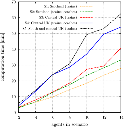
Figure 7: Computation time against number of agents

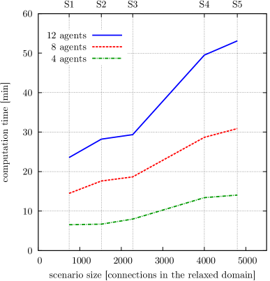
Figure 8: Computation time against scenario size

5.3.2 Success rate

To assess the value of the algorithm, we also need to look at how many agents end up having a valid travel plan. Planning in the relaxed domain in the initial and the BR phase of the algorithm is very successful. After the BR phase, 99.4 % of agents have a journey plan. The remaining 0.6 % of all agents does not have a single-agent plan because of the irregularities in the relaxed domain caused by splitting the public transportation network into regions. The agents without a single-agent plan are not matched to timetable connections in the timetabling phase.

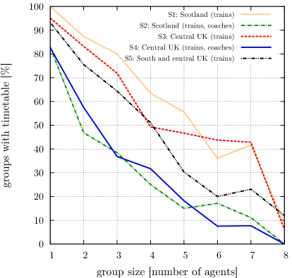
Figure 9: Percentage of groups for which a timetable was found as a function of group size.

The timetabling phase is of course much more problematic. Figure 9 shows the percentage of groups for which a timetable was found, as a function of group size. In order to create this graph, number of groups with assigned timetable and total number of groups identified was counted for every size of the group. There are several things to point out here.

Naturally, the bigger a group is, the harder it is to find a feasible timetable, as the problem quickly becomes overconstrained in terms of travel times and actually available transportation services. When a group of agents sharing parts of their journeys is big (5 or more agents), the percentage of groups for which we can find a timetable drops below 50 %. With a group of 8 agents, almost no timetable can be found. Basically what happens here is that the initial and BR phases find suitable ways of travelling together in principle, but that it becomes impossible to find appropriate connections that satisfy every traveller’s requirements, or do not add up to a total duration of less than 24 hours.

We can also observe that the success rate is higher in scenarios that use only trains than in those that combine trains and coaches. On closer inspection, we can observe that this is mainly caused by different service densities in the rail and coach networks, i.e., the ratios of timetabled connections over connections in the relaxed domain. For example, the service density is 33 train services a day compared to only 4 coach services in Scotland. As a consequence, it is much harder to find a timetable in a scenario with both trains and coaches because the timetable of coaches is much less regular than the timetable of trains. However, this does not mean that there is less sharing if coaches are included. Instead, it just reflects the fact that due to low service density, many of the envisioned shared journeys do not turn out to be feasible using coaches. The fact that this cannot be anticipated in the initial and BR phases is a weakness of our method, and is discussed further in section 7.

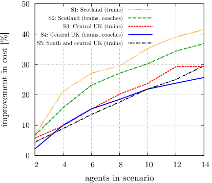
Figure 10: Average cost improvement

Figure 11: Percentage of groups with less than 30 % journey prolongation

5.3.3 Plan quality

Finally, we want to assess the quality of the plans obtained with respect to improvement in cost of agents’ journeys and their prolongation, to evaluate the net benefit of using our method in the travel sharing domain. We should mention that the algorithm does not explicitly optimises the solutions with respect to these metrics. To calculate cost improvement, recalling that $C_{i}(\pi)=\sum_{j}c_{i}(a^{j})$ for a plan is the cost of a plan $\pi=\langle a^{1},\ldots,a^{k}\rangle$ to agent $i$, assume $n(a^{j})$ returns the number of agents with whom the $j$th step of the plan is shared. We can define a cost of a shared travel plan $C_{i}^{{}^{\prime}}(\pi)=\sum_{j}c_{i,n(a^{j})}(a^{j})$ using equation (1). With this we can calculate the improvement $\Delta C$ as follows:

$$\Delta C=\frac{\sum_{i\in N}C_{i}(\pi_{i})-\sum_{i\in N}C_{i}^{{}^{\prime}}(\pi_{N})}{\sum_{i\in N}C_{i}(\pi_{i})}$$ (2)

where $N$ is the set of all agents, $\pi_{i}$ is the single-agent plan initially computed for agent $i$, and $\pi_{N}$ is the final joint plan of all agents after completion of the algorithm (which is interpreted as the plan of the “grand coalition” $N$ and reflects how subgroups within $N$ share parts of the individual journeys).

The average cost improvement obtained in our experiments is shown in Figure 10, and it shows that the more agents there are in the scenario, the higher the improvement. However, there is a trade-off between the improvement in cost and the percentage of groups that we manage to find a suitable timetable for, cf. Figure 9.

On the one hand, travel sharing is beneficial in terms of cost. On the other hand, a shared journey has a longer duration than a single-agent journey in most cases. In order to evaluate this trade-off, we also measure the journey prolongation. Assume that $T_{\mathrm{i}}(\pi)$ is the total duration of a plan to agent $i$ in plan $\pi$, and, as above, $\pi_{i}$/$\pi_{N}$ denote the initial single-agent plans and the shared joint plan at the end of the timetabling phase, respectively. Then, the prolongation $\Delta T$ of a journey is defined as follows:

$$\Delta T=\frac{\sum_{i\in N}T_{i}(\pi_{N})-\sum_{i\in N}T_{i}(\pi_{i})}{\sum_{i\in N}T_{i}(\pi_{i})}$$ (3)

Journey prolongation can be calculated only when a group is assigned a timetable and each member of the group is assigned a single-agent timetable. For this purpose, in every experiment, we also calculate single-agent timetables in the timetabling phase of the algorithm.

A graph of the percentage of groups that have a timetable with prolongation less than 30 % as a function of group size is shown in Figure 11. The graph shows which groups benefit from travel sharing, i.e., groups whose journeys are not prolonged excessively by travelling together. Approximately 15 % of groups with 3–4 agents are assigned a timetable that leads to a prolongation of less than 30 %. Such a low percentage of groups can be explained by the algorithm trying to optimise the price of the journey by sharing in the BR phase. However, there is a trade-off between the price and the duration of the journey. The more agents are sharing a journey, the longer the journey duration is likely to be.

These results were obtained based on the specific cost function (1) we have introduced to favour travel sharing, and which would have to be adapted to the specific cost structure that is present in a given transportation system. Also, the extent to which longer journey times are acceptable for the traveller depends on their preferences, but these could be easily adapted by using different cost functions.

6 Discussion

The computation of single-agent plans in the initial phase involves solving a set of completely independent planning problems. This means that the planning process could be speeded up significantly by using parallel computation on multiple CPUs. The same is true for matching different independent groups of agents to timetabled connections in the timetabling phase. As an example, assume that there are $N$ agents in the scenario and $t_{1},\dots,t_{N}$ are the computation times for respective single-agent initial plans. If computed concurrently, this would reduce the computation time from $t=\sum_{i=1}^{N}t_{i}$ to $t^{\prime}=\max_{i=1}^{N}(t_{i})$. Similar optimisations could be performed for the timetabling phase of the algorithm. In the experiments with 10 agents, for example, this would lead to a runtime reduced by 48 % in scenario S1 and by 44 % in scenario S5.

A major problem of our method is the inability to find appropriate connections in the timetabling phase for larger groups. There are several reasons for this. Firstly, the relaxed domain is overly simplified, and many journeys found in it do not correspond to journeys that would be found if we were planning in the full domain. Secondly, there are too many temporal constraints in bigger groups (5 or more agents), so the timetable matching problem becomes unsolvable given the 24-hour timetable. However, it should also be pointed out that such larger groups would be very hard to identify and schedule even using human planning. Thirdly, some parts of public transportation network have very irregular timetables.

Our method clearly improves the cost of agents’ journeys by sharing parts of the journeys, even though there is a trade-off between the amount of improvement, the percentage of found timetables and the prolongation of journeys. On the one hand, the bigger the group, the better the improvement. On the other hand, the more agents share a journey, the harder it is to match their joint plan to timetable. Also, the prolongation is likely to be higher with more agents travelling together, and will most likely lead to results that are not acceptable for users in larger groups.

Regarding the domain-independence of the algorithm, we should point out that its initial and BR phases are completely domain-independent so they could easily be used in other problem domains such as logistics, network routing or service allocation. In the traffic domain, the algorithm can be used to plan routes that avoid traffic jams or to control traffic lights. What is more, additional constraints such as staying at one city for some time or travelling together with a specific person can be easily added. On the other hand, the timetabling phase of the algorithm is domain-specific, providing an example of the specific design choices that have to be made from an engineering point of view.

To assess the practical value of our contribution, it is worth discussing how it could be used in practice as a part of a travel planning system for real passengers. In such a system, every user would submit origin, destination and travel times. Different users could submit their preferences at different times, with the system continuously computing shared journeys for them based on information about all users’ preferences. Users would need to agree on a shared journey in time to arrange meeting points and to purchase tickets, subject to any restrictions on advance tickets etc. Because of this lead time, it would be entirely sufficient if the users got an e-mail with a planned journey one hour after the last member of the travel group submits his or her journey details, which implies that even with our current implementation of the algorithm, the runtimes would be acceptable.

From our experimental evaluation, we conclude that reasonable group sizes range from two to four persons. Apart from the fact that such groups can be relatively easily coordinated, with the price model used in this paper, cf. formula (1), every member of a three-person group could save up to 53 % of the single-agent price. The success rate of the timetabling phase of the algorithm for three-person groups in the scenario S3 (trains in the central UK) is 70 %.

7 Conclusion

We have presented a multiagent planning algorithm which is able to plan meaningful shared routes in a real-world travel domain. The algorithm has been implemented and evaluated on five scenarios based on real-world UK public transport data. The algorithm exhibits very good scalability, since it scales linearly both with the scenario size and the number of agents. The average computation time for 12 agents in the scenario with 90 % of trains in the UK is less than one hour. Experiments indicate that the algorithm avoids the exponential blowup in the action space characteristic for a centralised multiagent planner.

To deal with thousands of users that could be in a real-world travel planning system, a preprocessing step would be needed: The agents would have to be divided into smaller groups by clustering them according to departure time, direction of travel, origin, destination, length of journey and preferences (e.g., travel by train only, find cheapest journey). Then, the algorithm could be used to find a shared travel plan with a timetable. To prevent too large groups of agents which are unlikely to be matched to the timetable, a limit can be imposed on the size of the group. If a group plan cannot be mapped to a timetable, the group can be split into smaller sub-groups which are more likely to identify a suitable timetable.

Finally, the price of travel and flexibility of travel sharing can be significantly improved by sharing a private car. In the future, we would like to explore the problem of planning shared journeys when public transport is combined with ride sharing. Then, in order to have a feasible number of nodes in the travel domain, train and bus stops can be used as meeting points where it is possible to change from a car to public transport or vice versa.

8 Acknowledgments

Partly supported by the Ministry of Education, Youth and Sports of Czech Republic (grant No. LD12044) and European Commission FP7 (grant agreement No. 289067).

References

- [1] S. Abdel-Naby, S. Fante, and P. Giorgini. Auctions Negotiation for Mobile Rideshare Service. In Procs. ICPCA 2007, pages 225–230, 2007.
- [2] R. I. Brafman and C. Domshlak. From One to Many: Planning for Loosely Coupled Multi-Agent Systems. In Procs. ICAPS 2008, pages 28–35. AAAI Press, 2008.
- [3] R. I. Brafman, C. Domshlak, Y. Engel, and M. Tennenholtz. Planning Games. In Procs. IJCAI 2009, pages 73–78, July 2009.
- [4] Y. Chen, B. W. Wah, and C.-W. Hsu. Temporal planning using subgoal partitioning and resolution in SGPlan. Journal of Artificial Intelligence Research, 26:323–369, Aug. 2006.
- [5] A. J. Coles, A. I. Coles, A. Clark, and S. T. Gilmore. Cost-Sensitive Concurrent Planning under Duration Uncertainty for Service Level Agreements. In Procs. ICAPS 2011, pages 34–41. AAAI Press, June 2011.
- [6] A. J. Coles, A. I. Coles, M. Fox, and D. Long. Forward-Chaining Partial-Order Planning. In Procs. ICAPS 2010, pages 42–49. AAAI Press, May 2010.
- [7] A. J. Coles, A. I. Coles, M. Fox, and D. Long. POPF2: a Forward-Chaining Partial Order Planner. In Procs. IPC-7, 2011.
- [8] E. Ferrari, R. Manzini, A. Pareschi, A. Persona, and A. Regattieri. The car pooling problem: Heuristic algorithms based on savings functions. Journal of Advanced Transportation, 37(3):243–272, 2003.
- [9] M. Ghallab, D. Nau, and P. Traverso. Automated Planning: Theory and Practice. Morgan Kaufmann Publishers Inc., 2004.
- [10] J. Hoffmann and B. Nebel. The FF planning system: Fast plan generation through heuristic search. Journal of Artificial Intelligence Research, 14:253–302, 2001.
- [11] J. Hrnčíř. Improving a Collaborative Travel Planning Application. Master’s thesis, The University of Edinburgh, Aug. 2011.
- [12] C.-W. Hsu and B. W. Wah. The SGPlan Planning System in IPC-6. In Procs. IPC-6, 2008.
- [13] A. Jonsson and M. Rovatsos. Scaling Up Multiagent Planning: A Best-Response Approach. In Procs. ICAPS 2011, pages 114–121. AAAI Press, June 2011.
- [14] P. Lalos, A. Korres, C. K. Datsikas, G. S. Tombras, and K. Peppas. A Framework for Dynamic Car and Taxi Pools with the Use of Positioning Systems. In Computation World: Future Computing, Service Computation, Cognitive, Adaptive, Content, Patterns, pages 385–391, Nov. 2009.
- [15] N. Meuleau, M. Hauskrecht, K.-E. Kim, L. Peshkin, L. P. Kaelbling, T. Dean, and C. Boutilier. Solving very large weakly coupled Markov decision processes. In Procs. AAAI 1998, pages 165–172. AAAI Press, 1998.
- [16] D. Monderer and L. S. Shapley. Potential Games. Games and Economic Behavior, 14(1):124–143, 1996.
- [17] S. Richter, M. Helmert, and M. Westphal. Landmarks Revisited. In Procs. AAAI 2008, pages 975–982. AAAI Press, July 2008.
- [18] S. Richter and M. Westphal. The LAMA planner. Using landmark counting in heuristic search. In Procs. IPC-6, 2008.
- [19] B. W. Wah and Y. Chen. Constraint partitioning in penalty formulations for solving temporal planning problems. Artificial Intelligence, 170:187–231, Mar. 2006.