Combinatorial Heegaard Floer homology and sign assignments

Abstract.

We provide an intergral lift of the combinatorial definition of Heegaard Floer homology for nice diagrams, and show that the proof of independence using convenient diagrams adapts to this setting.

1. Introduction

In [4, 5] various versions of Heegaard Floer homology groups were defined for oriented, closed 3–manifolds. The construction of these invariants relied on a Heegaard diagram of the 3–manifold, and applied a suitably adapted variant of Lagrangian Floer homology to a symplectic manifold associated to the Heegaard diagram. Consequently, both the definition of the group and the verification of its topological invariance involved (almost–)complex analytic arguments. The homology groups come with additional structures, such as a decomposition according to spin^c structures of the 3–manifold, and an absolute ${\mathbb{Q}}$–grading of those groups which correspond to torsion spin^c structures. The theories can be most easily defined over the base field $\mathbb{F}=\mathbb{Z}/2\mathbb{Z}$; but, with the help of coherent orientation systems, they also admit a definition over $\mathbb{Z}$. For the purposes of three-dimensional topological applications, the theory over $\mathbb{F}$ is often sufficient. For four-dimensional applications, most notably those using the mixed invariant defined in [6], however, the integral valued theory is much more powerful than its mod $2$ reduced counterpart.

In [9] Sarkar and Wang found a combinatorial way for computing the simplest version, ${\widehat{\rm{HF}}}$ of the Heegaard Floer homology groups over the field $\mathbb{F}={\mathbb{Z}}/2{\mathbb{Z}}$. Their idea was to use Heegaard diagrams with a particular combinatorial structure, called nice diagrams, in the computation of the Heegaard Floer homology of a given 3–manifold $Y$. For such diagrams the (almost–)holomorphic computations reduce to simple combinatorics. They also showed that any 3–manifold admits a nice diagram. In [3], the present authors described certain specific nice diagrams. With the help of these convenient diagrams, we verified the independence of the (stable) Heegaard Floer homology groups from the choice of the diagram, using a purely topological argument. In [3, 9] only $\mathbb{Z}/2\mathbb{Z}$–coefficients were used.

In the present work we extend the combinatorial/topological approach from [3], to provide a combinatorial definition of the (stable) ${\widehat{\rm{HF}}}$–version over $\mathbb{Z}$. To state our main results, we first recall the basics of the definition of Heegaard Floer homology groups.

Suppose that $\mathfrak{D}=(\Sigma,\mbox{\boldmath$\alpha$},\mbox{\boldmath$\beta$},\mathbf{w})$ is a given nice multi-pointed Heegaard diagram of a 3–manifold $Y$. The Heegaard Floer chain complex $({\widetilde{\rm{CF}}}(\mathfrak{D}),{\widetilde{\partial}}_{\mathfrak{D}})$ of $\mathfrak{D}$ over $\mathbb{Z}/2\mathbb{Z}$ is defined by considering the $\mathbb{Z}/2\mathbb{Z}$–vector space generated by the generators, i.e. $n$–tuples $\mathbf{x}=\{x_{1},\ldots,x_{n}\}\subset\Sigma$ with the property that each $\alpha_{i}\in\mbox{\boldmath$\alpha$}$ and each $\beta_{j}\in\mbox{\boldmath$\beta$}$ contains exactly one element of $\mathbf{x}$. The boundary operator ${\widetilde{\partial}}_{\mathfrak{D}}$ is the linear map ${\widetilde{\rm{CF}}}(\mathfrak{D})\to{\widetilde{\rm{CF}}}(\mathfrak{D})$ given by the matrix element $\langle{\widetilde{\partial}}_{\mathfrak{D}}\mathbf{x},\mathbf{y}\rangle$, which is equal to the mod 2 count of flows (i.e., empty bigons or empty rectangles) from $\mathbf{x}$ to $\mathbf{y}$. (For a more detailed treatment see [3, Section 6].) The map ${\widetilde{\partial}}_{\mathfrak{D}}$ then satisfies ${\widetilde{\partial}}_{\mathfrak{D}}^{2}=0$. In [3] we showed that the homology of the resulting chain complex is (stably) invariant under nice moves. In [3] it was also shown that specific nice diagrams (called convenient) can be connected by sequences of nice moves. This result then completed the proof of the topological invariance of the stable groups. (For a more detailed description of these notions see [3].)

The definition above can be adapted to the setting over $\mathbb{Z}$: now ${\widetilde{\rm{CF}}}(\mathfrak{D};\mathbb{Z})$ is generated by the same set of generators over $\mathbb{Z}$, while the matrix element $\langle{\widetilde{\partial}}_{\mathfrak{D}}\mathbf{x},\mathbf{y}\rangle$ of the boundary map ${\widetilde{\partial}}_{\mathfrak{D}}^{\mathbb{Z}}$ counts the empty bigons and empty rectangles with certain sign. The aim of this paper is to describe a sign assignment for these objects which has two crucial properties: (1) the resulting operator ${\widetilde{\partial}}^{\mathbb{Z}}_{\mathfrak{D}}$ satisfies $({\widetilde{\partial}}^{\mathbb{Z}}_{\mathfrak{D}})^{2}=0$, and (2) the homology of the resulting chain complex is (stably) invariant under nice moves.

Our strategy is as follows: we first define formal generators and formal flows, which capture certain combinatorial features of actual generators and flows associated to a Heegaard diagram. (We use the term flow loosely to refer to those objects which are counted in the Heegaard Floer differential.) For a fixed positive integer $n$, in Section 2 we will define the set ${\mathcal{G}}_{n}$ of formal generators. The set ${\mathcal{F}}_{n}$ (also to be defined in Section 2) will consist of formal flows connecting pairs of formal generators from ${\mathcal{G}}_{n}$. After fixing some extra data, such as orientations on the $\alpha$– and $\beta$–curves and an order on them, an intersection point (and a flow) in a Heegaard diagram having $n$ $\alpha$– and $n$ $\beta$–curves naturally gives rise to a formal generator in ${\mathcal{G}}_{n}$ (and a formal flow in ${\mathcal{F}}_{n}$, respectively).

A sign assignment is a map $S\colon{\mathcal{F}}_{n}\to\{\pm 1\}$ which satisfies certain properties (to be spelled out in Definition 2.5). By applying simple modifications (see Definition 2.6) to a given sign assignment, we can produce further sign assignments, which will be called gauge equivalent to the original sign assignment. The main result of the present paper is

Theorem 1.1.

For a given positive integer $n$ there exists a sign assignment $S\colon{\mathcal{F}}_{n}\to\{\pm 1\}$, and it is unique up to gauge equivalence.

Resting on this result, for a nice Heegaard diagram $\mathfrak{D}$ and a sign assignment $S$ we will show:

Theorem 1.2.

The map ${\widetilde{\partial}}_{\mathfrak{D}}^{\mathbb{Z}}$ over $\mathbb{Z}$ defined using the fixed sign assignment $S$ satisfies $({\widetilde{\partial}}_{\mathfrak{D}}^{\mathbb{Z}})^{2}=0$ and the resulting homology ${\widetilde{\rm{HF}}}(\mathfrak{D};\mathbb{Z})$ is independent of the choice of $S$, of the chosen orientations and order of the $\alpha$– and $\beta$–curves. Moreover ${\widetilde{\rm{HF}}}(\mathfrak{D};\mathbb{Z})$ is (stably) invariant under nice moves.

As an application of the theorem above, we will show that the stable Heegaard Floer homology ${\widehat{\rm{HF}}}_{{\rm{st}}}(Y)$ of a 3–manifold $Y$ (as it is defined in [3]) admits an integral lift over $\mathbb{Z}$ and provides a diffeomorphism invariant ${\widehat{\rm{HF}}}_{{\rm{st}}}(Y;\mathbb{Z})$ of closed, oriented 3–manifolds; cf. Corollary 3.8.

The paper is organized as follows. In Section 2 we introduce the necessary formal notions and define sign assignments. To give a better picture about these objects, we also work out two examples (for powers $n=1,2$). In Section 3 we apply the existence and uniqueness result of sign assignments and verify the independence of the Heegaard Floer homology groups over $\mathbb{Z}$ from the necessary choices, leading us to the proof of Theorem 1.2. Finally, in Section 4 we prove Theorem 1.1.

Acknowledgements: PSO was supported by NSF grant number DMS-0804121. AS was supported by OTKA NK81203 and by Lendület project of the Hungarian Academy of Sciences. He also wants to thank the Institute for Advanced Study for their hospitality. ZSz was supported by NSF grant numbers DMS-0704053 and DMS-1006006. We would like to thank the Mathematical Sciences Research Institute, Berkeley for providing a productive research enviroment.

2. Sign assignments

For the definition of the formal generators and formal flows fix a positive integer $n$ and two $n$-element sets $\alpha$ and $\beta$. (In the following discussion $n$ will be referred to as the power of the formal generators, flows and the sign assignments we will define with the use of the sets $\alpha$ and $\beta$.)

Definition 2.1.

A formal generator is a one-to-one correspondence $\rho$ between the sets $\alpha$ and $\beta$ (which we think of as a subset of the Cartesian product $\mbox{\boldmath$\alpha$}\times\mbox{\boldmath$\beta$}$), together with a function $\zeta$ from $\rho$ to $\{\pm 1\}$.

More concretely, after fixing orderings of the elements of $\alpha$ and $\beta$, $\mbox{\boldmath$\alpha$}=\{\alpha_{1},\dots,\alpha_{n}\}$ and $\mbox{\boldmath$\beta$}=\{\beta_{1},\dots,\beta_{n}\}$, the one-to-one correspondence $\rho$ can be thought of as a permutation $\sigma$ of $\{1,\dots,n\}$, via the convention that $\rho=\{(\alpha_{i},\beta_{\sigma(i)})\}_{i=1}^{n}\subset\mbox{\boldmath$\alpha$}\times\mbox{\boldmath$\beta$}$. Similarly, the function $\zeta$ can be encoded in an $n$-tuple $\epsilon=(\epsilon_{1},\dots,\epsilon_{n})\in\{\pm 1\}^{n}$, with the convention that $\epsilon_{i}=\zeta(\alpha_{i},\beta_{\sigma(i)})$. We call $\sigma$ the associated permutation, and $\epsilon\in\{\pm 1\}^{n}$ the sign profile of the formal generator. With respect to this choice we write formal generators as pairs $(\epsilon,\sigma)$. For the fixed integer $n$ the set of formal generators of power $n$ will be denoted by ${\mathcal{G}}_{n}$. It follows from the above definition that ${\mathcal{G}}_{n}$ has $n!\cdot 2^{n}$ elements.

A pictorial way of defining formal generators is given by considering $n$ disjoint crosses on the plane, where at each of the crossing points the two arcs are equipped with an orientation and decorated with one of the $\alpha_{i}$ or $\beta_{j}$. (Each arc is decorated by a different $\alpha_{i}$ or $\beta_{j}$.) We consider two such pictures identical if there is an orientation preserving self-diffeomorphism of the plane mapping one picture to the other, respecting both the labelings and the orientations of the arcs in the crosses. The sign of the crossing (with the convention that the $\alpha$–curve comes first and the plane is oriented by the counterclockwise rotation) determines the sign profile. For a particular example see Figure 1. It is rather simple to derive the abstract description of a formal generator from its pictorial presentation.

Figure 1. A pictorial presentation of a formal generator. We depict a generator for $n=5$. This generator corresponds to the permutation $(142)(35)$ and its sign profile is the constant $-1$ function.

Now we turn to the definition of formal flows. This will be done in two steps: we will first define formal bigons and then formal rectangles.

Definition 2.2.

For a fixed positive integer $n$ and sets $\mbox{\boldmath$\alpha$}=\{\alpha_{1},\ldots,\alpha_{n}\}$, $\mbox{\boldmath$\beta$}=\{\beta_{1},\ldots,\beta_{n}\}$ consider $n-1$ pairs of oriented arcs in the plane intersecting each other in each pair exactly once, and otherwise disjoint. Consider a further pair of oriented arcs, intersecting each other in two points, and disjoint from all the crossings. The complement of the last two arcs has two components (one compact and one non-compact); the first $n-1$ pairs are all required to be in the non-compact component. Decorate one of the arcs in each pair with an $\alpha_{i}$ and the other one with a $\beta_{j}$ in such a manner that each element of $\alpha$ and of $\beta$ is used exactly once. Two such configurations are considered to be equivalent if there is an orientation preserving diffeomorpism of the plane mapping one into the other, while respecting both the orientations and the decorations of the arcs. An equivalence class of such objects is called a formal bigon. For a pictorial presentation of a formal bigon, see Figure 2.

Figure 2. A formal bigon. The bigon in the diagram connects two formal generators for $n=5$. The two formal generators connected by the formal bigon are represented by the full and hollow circles, respectively. In the above example the formal bigon points from the generator represented by full circles to the one represented by hollow circles.

A formal bigon determines two formal generators $\mathbf{x}$ and $\mathbf{y}$ by adding the small neighbourhood of one of the crossings of the last two arcs (intersecting each other twice) to the first $n-1$ crosses, with the induced orientations and decorations. The formal bigon is from $\mathbf{x}$ to $\mathbf{y}$ (denoted by $b\colon\mathbf{x}\to\mathbf{y}$) if the orientation of the plane restricted to the compact domain encircled by the last two arcs induces an orientation on the arc with the $\alpha$-decoration pointing from the $\mathbf{x}$-coordinate towards the $\mathbf{y}$–coordinate. The four possible formal bigons for $n=1$ are illustrated in Figure 3.

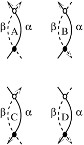
Figure 3. The four formal bigons for $n=1$. Each bigon points from the formal generator denoted by the full circle to the one denoted by the hollow circle. In this diagram the $\beta$-arcs are distinguished from the $\alpha$-arcs by being drwan as dashed curves.

Notice that the two formal generators $\mathbf{x}$ and $\mathbf{y}$ connected by a formal bigon $b$ have identical associated permutations, while the sign profiles of $\mathbf{x}$ and $\mathbf{y}$ differ in exactly one coordinate (given by the labels of the $\alpha$ and $\beta$ curve corresponding to the arcs intersecting each other twice). We say that the bigon $b$ is supported in this coordinate, or that is its moving coordinate. For a given $n$ there are $2n\cdot n!\cdot 2^{n}$ formal bigons: there are $n!\cdot 2^{n}$ choices for the starting formal generator, $n$ choices for the moving coordinates and 2 further possibilities as how the bigon starts at the selected crossing containing the moving coordinates. We make the following analogous definitions for rectangles:

Definition 2.3.

For a fixed positive integer $n$ and sets $\mbox{\boldmath$\alpha$}=\{\alpha_{1},\ldots,\alpha_{n}\}$, $\mbox{\boldmath$\beta$}=\{\beta_{1},\ldots,\beta_{n}\}$ consider $n-2$ pairs of oriented arcs in the plane intersecting each other in each pair exactly once, and otherwise disjoint. Consider furthermore two pairs of oriented closed arcs $(a_{1},b_{1})$ and $(a_{2},b_{2})$ such that $a_{1}$ and $a_{2}$ (and likewise $b_{1}$ and $b_{2}$) are disjoint, while both $a_{i}$ intersects both $b_{j}$ exactly once in their interiors. One of the two components of the complement is compact, and we require its interior to be disjoint from all the other arcs. Decorate one of the arcs in each pair with an $\alpha_{i}$ and the other one with a $\beta_{j}$ in such a manner that each element of $\alpha$ and of $\beta$ is used exactly once; the $a_{i}$ arcs in the rectangle will be decorated by elements of $\alpha$ while the $b_{j}$ arcs with elements of $\beta$. Two such configurations are considered to be equivalent if there is an orientation preserving diffeomorpism of the plane mapping one into the other, while respecting both the orientations and the decorations of the arcs. An equivalence class of such objects is called a formal rectangle. For a pictorial presentation of a formal rectangle see Figure 4.

Figure 4. A formal rectangle. Once again, the rectangle given by the diagram is a formal flow for $n=5$. The rectangle points from the full circles to the hollow circles.

Notice that the last two pairs of arcs (provided that are made of straight line segments) form a rectangle with four vertices. The formal rectangle determines two formal generators $\mathbf{x}$ and $\mathbf{y}$, where the first $n-2$ coordinates coming from the crosses are completed by the neighbourhoods of two opposite vertices of the above rectangle. Once again, using the restriction of the orientation of the plane, we say that the formal rectangle $r$ is from $\mathbf{x}$ to $\mathbf{y}$ (and write $r\colon\mathbf{x}\to\mathbf{y}$) if the induced orientation on the sides of the rectangle labeled by $\alpha$ (viewed as part of the boundary of the compact component of the complement) point from the $\mathbf{x}$-coordinate to the $\mathbf{y}$-coordinate. Notice also that the associated permutations for $\mathbf{x}$ and $\mathbf{y}$ differ by a transposition, and the coordinates in the transposition are the moving coordinates of the rectangle. It is easy to determine the number of formal rectangles when $|\mbox{\boldmath$\alpha$}|=|\mbox{\boldmath$\beta$}|=n$: there are $n!\cdot 2^{n}$ starting points of a rectangle, and once this is fixed, we have $\frac{1}{2}n(n-1)$ possibilities to choose the moving coordinates. In addition, there are 2 ways at each of the two starting coordinates the rectangle can start. Altogether it shows that there are $2n\cdot(n-1)\cdot n!\cdot 2^{n}$ formal rectangles of power $n$.

Definition 2.4.

A formal flow is, by definition, either a formal bigon or a formal rectangle. For a given positive integer $n$ the set of formal flows connecting elements of the set ${\mathcal{G}}_{n}$ of formal generators will be denoted by ${\mathcal{F}}_{n}$.

The sign assignment we are looking for is a map from ${\mathcal{F}}_{n}$ to $\{\pm 1\}$ which satisfies certain relations, which we describe now. Consider one of the diagrams of Figure 5.

Figure 5. Two pairs of formal flows giving rise to boundary degenerations. The diagram on the left shows a disk-like, while on the right an annular boundary degeneration. In both cases we can equip the curves with arbitrary orientations, and decorations from the sets $\alpha$ and $\beta$. As always, curves with the same type of decorations should be disjoint.

Suppose that, with some orientations and after decorating the arcs with $\alpha_{i}$ and $\beta_{j}$ (and adding the oriented, decorated crossings), Figure 5(a) or (b) represent two formal flows $\phi_{1}$ and $\phi_{2}$. Then we say that the pair $(\phi_{1},\phi_{2})$ is a boundary degeneration. The type of the degeneration is $\alpha$ or $\beta$, depending on the decoration of the circle(s) in the figure. Sometimes we say that in case (a) the degeneration is disk-like, while in (b) it is annular. Notice that if $\phi_{1}$ and $\phi_{2}$ are two formal flows which give a pair of boundary degeneration, and $\phi_{1}$ is a formal flow from one formal generator $(\epsilon_{1},\sigma_{1})$ to another one $(\epsilon_{2},\sigma_{2})$ then $\phi_{2}$ is a formal flow from $(\epsilon_{2},\sigma_{2})$ back to $(\epsilon_{1},\sigma_{1})$.

Similarly, consider a pair of formal flows $(\phi_{1},\phi_{2})$ with the property that $\phi_{1}$ goes from $(\epsilon_{1},\sigma_{1})$ to $(\epsilon_{2},\sigma_{2})$, while $\phi_{2}$ goes from $(\epsilon_{2},\sigma_{2})$ to $(\epsilon_{3},\sigma_{3})$, and now assume that $(\epsilon_{1},\sigma_{1})$ is different from $(\epsilon_{3},\sigma_{3})$. We distinguish two cases. First, if the coordinates which move under $\phi_{1}$ are different from the ones moving under $\phi_{2}$, then we can switch the order of these flows to provide two further flows $\phi_{3}\colon(\epsilon_{1},\sigma_{1})\to(\epsilon_{2}^{\prime},\sigma_{2}^{\prime})$ and $\phi_{4}\colon(\epsilon_{2}^{\prime},\sigma_{2}^{\prime})\to(\epsilon_{3},\sigma_{3})$: $\phi_{3}$ is uniquely determined by the properties that it has the same initial point as $\phi_{1}$ but the moving coordinates of $\phi_{2}$, whereas $\phi_{4}$ has the same terminal point as $\phi_{2}$ but the same moving coordinates as $\phi_{1}$. In this case, we say that the two pairs $(\phi_{1},\phi_{2})$ and $(\phi_{3},\phi_{4})$ form a square. In case there are moving coordinates shared by $\phi_{1}$ and $\phi_{2}$, we consider one of the diagrams of Figure 6 (equipped with all possible $\alpha_{i}$- and $\beta_{j}$-curves and orientations, and extended by all possible oriented crossings), which define the corresponding pair of formal flows $(\phi_{3},\phi_{4})$. Once again, in such a situation we say that the pairs $(\phi_{1},\phi_{2})$ and $(\phi_{3},\phi_{4})$ form a square. Now we are in the position of giving the definition of a sign assignment.

Figure 6. Diagrams describing flows sharing moving coordinates. The curve segments can be equipped with arbitrary orientations, labelings and extensions with further crossings to define squares of flow lines $\{(\phi_{1},\phi_{2}),(\phi_{3},\phi_{4})\}$.

Definition 2.5.

Fix a positive integer $n$. A sign assignment $S$ of power $n$ is a map from the set of all formal flows ${\mathcal{F}}_{n}$ into $\{\pm 1\}$ with the following properties:

• if $(\phi_{1},\phi_{2})$ is an $\alpha$-type boundary degeneration, then

  $$S(\phi_{1})\cdot S(\phi_{2})=1;$$

• if $(\phi_{1},\phi_{2})$ is a $\beta$-type boundary degeneration, then

  $$S(\phi_{1})\cdot S(\phi_{2})=-1;$$

• if the two pairs $(\phi_{1},\phi_{2})$ and $(\phi_{3},\phi_{4})$ form a square, then

  $$S(\phi_{1})\cdot S(\phi_{2})+S(\phi_{3})\cdot S(\phi_{4})=0.$$

Notice that this last requirement is equivalent to requiring the identity $\Pi_{i=1}^{4}S(\phi_{i})=-1$ to hold.

There is a simple operation for constructing new sign assignments from an old one.

Definition 2.6.

If $S\colon{\mathcal{F}}_{n}\to\{\pm 1\}$ is a sign assignment, and $u$ is any map $u\colon{\mathcal{G}}_{n}\to\{\pm 1\}$, then we can define a new sign assignment $S^{u}$ as follows: if $\phi\colon\mathbf{x}\to\mathbf{y}$ is a formal flow from $\mathbf{x}$ to $\mathbf{y}\in{\mathcal{G}}_{n}$, then let $S^{u}(\phi)=u(\mathbf{x})\cdot S(\phi)\cdot u(\mathbf{y})$. If $S$ and $S^{u}$ are related in this way, we say that $S$ and $S^{u}$ are gauge equivalent sign assignments and $u$ will be called a gauge transformation. The function $u\colon{\mathcal{G}}_{n}\to\{\pm 1\}$ is a restricted gauge transformation if $u(\mathbf{x})$ depends only on the permutation corresponding to the formal generator $\mathbf{x}$ (and is independent of its sign profile).

Since in each relation of Definition 2.5 for $S^{u}$ any $u(\mathbf{x})$ appears an even number of times, the fact that $S^{u}$ is a sign assignment follows trivially from the fact that $S$ is a sign assignment. With these definitions in place, we have the precise version of Theorem 1.1:

Theorem 2.7.

For any integer $n$ there is, up to gauge equivalence, a unique sign assignment on ${\mathcal{F}}_{n}$.

Remark 2.8.

The definition of a sign assignment shows a certain asymmetry between the $\alpha$ and $\beta$ curves in the degeneration rule. Let $m\colon{\mathcal{G}}_{n}\to\{\pm 1\}$ denote the map which associates to each formal generator $(\sigma,\epsilon)$ the product $sgn(\sigma)\cdot\Pi\epsilon_{i}$, where $sgn(\sigma)$ is the parity of the permutation (and is $1$ for even and $-1$ for odd permutations) and $\epsilon_{i}$ are the coordinates of the sign profile $\epsilon$. Then the formula $S^{\prime}(\phi)=S(\phi)\cdot m(\mathbf{x})$ for a formal flow $\phi\in{\mathcal{F}}_{n}$ from $\mathbf{x}$ to $\mathbf{y}$ and for a signs assignment $S$ defines a map $S^{\prime}\colon{\mathcal{F}}_{n}\to\{\pm 1\}$ which satisfies the axioms of a sign assignment provided the roles of $\alpha$ and $\beta$ are switched.

There are a number of further types of squares $\{(\phi_{1},\phi_{2}),(\phi_{3},\phi_{4})\}$ with the property that $\phi_{1}$ and $\phi_{2}$ (and so also $\phi_{3}$ and $\phi_{4}$) share moving coordinates. In the diagrams of Figure 6 only a few such types are shown. It can be easily verified that if the relations required by Definition 2.5 are satisfied, then the relations presented by the further squares of Figure 7 follow:

Figure 7. Further squares of flows sharing moving coordinates.

Lemma 2.9.

Suppose that the square $\{(\phi_{1},\phi_{2}),(\phi_{3},\phi_{4})\}$ is defined by one of the diagrams of Figure 7. For a sign assignement $S$ then we have that

$$\Pi_{i=1}^{4}S(\phi_{i})=-1.$$

Proof.

The proof of this statement is a rather long but simple computation. Below we show it in one demonstrative case and leave the interested reader to complete the remaining cases.

Consider the situation depicted by Figure 7(a) and equip the edges with some orientation and decoration (see, for example, Figure 8(a)). With the notations of Figure 8 the relations of Figure 6 imply

$$S(XAB)\cdot S(Y)\cdot S(AB)\cdot S(XY)=-1,$$

$$S(XAB)\cdot S(UV)\cdot S(XUAB)\cdot S(V)=-1.$$

(Notice that a flow is specified by its initial generator and its support; above we only indicate the support while the initial generators follow from the order of the terms.) In addition, $XY$ and $AD$ differ by a $\beta$ boundary degeneration and the switch of the sign profile of the non-moving coordinate (which can be realized by anticommuting with an appropriate bigon), and the same difference applies to the pair $DC$ and $V$, while $Y$ and $UV$ are identical as formal flows. Putting all these together, and using the identity of (S-3) for the squares of Figure 8(b) and (c), the identity

$$S(AB)\cdot S(CD)\cdot S(AD)\cdot S(BC)=-1$$

follows at once. With the chosen orientation and decoration this is exactly the relation provided by Figure 8(a).

Figure 8. The proof of anticommutativity.

A similar argument verifies the result for the situation depicted by Figure 7(b). The identity for pairs shown by Figures 7(c) and (d) are even simpler: here we only need to apply boundary degenerations. (Details of these cases are left to the reader; for Figure 7(c) see also the discussion prior to Remark 2.11.) ∎

The proof of Theorem 2.7 (given in Section 4) is rather long. To give a better picture about our argument, below we summarize the main steps in the proof. It starts with the observation that both ${\mathcal{G}}_{1}$ and ${\mathcal{F}}_{1}$ are rather simple sets, hence for $n=1$ the construction (and the proof of uniqueness, up to gauge equivalence) of a sign assignment is an easy task. Indeed, we will present it in the subsection below. In the next step, using the $n=1$ case and the usual principle of signs in singular and simplicial homology, we verify the statement of Theorem 2.7 for the subset of ${\mathcal{F}}_{n}$ given by all formal bigons, cf. Subsection 4.1. Next we consider another subset of ${\mathcal{F}}_{n}$, the flows between formal generators with sign profile constant 1. These are necessarily formal rectangles, and these can be modelled in grid diagrams of the appropriate size. Sign assignments for certain specific rectangles in grids have been discussed in [2]; in Subsection 4.2 we extend that result to all the formal rectangles between generators of the fixed sign profile. Finally, in Subsection 4.3 we use the relations given by those squares which involve rectangles and bigons to extend the definition to rectangles with various sign profiles, and we arrive to the definition of a sign assignment (once a choice of it for bigons and rectangles among generators of constant 1 sign profile is fixed). The verification of the properties of a sign assignment listed in Definition 2.5 will conclude the proof of Theorem 2.7. We also note that in most of the proofs very similar statements must be checked for different, but rather similar objects and configurations. In these cases we typically pick representative cases, give the argument in detail for those, and only indicate the necessary modifications for the other cases (in case there are any significant necessary modifications).

The proof of Theorem 2.7 will be preceded by its main application in the proof of Theorem 1.2. Before turning to this application, however, we work out two specific cases of Theorem 2.7 for $n=1,2$.

2.1. Two examples

Lemma 2.10.

In the case $n=1$ there is a unique sign assignment $S_{0}$, up to gauge equivalence.

Proof.

Notice that for $n=1$ we only need to deal with formal bigons. We have two formal generators (differing in their sign profile), and these are connected by the four formal bigons $A,B,C,D$ shown in Figure 3.

Considering the possible decompositions of an $\alpha$-boundary degeneration, we conclude that $S(A)\cdot S(B)=1$ and $S(C)\cdot S(D)=1$. (This is gotten by taking an $\alpha$-circle cut in two along a $\beta$-arc, and considering the possible orientations of the circle and the arc.) Similarly, if we decompose $\beta$-boundary degenerations, we obtain the relations $S(A)\cdot S(C)=S(B)\cdot S(D)=-1$. Putting all these relations together, we conclude that

$$S(A)=S(B)=-S(C)=-S(D).$$

There are two possible such sign assignments, which are distinguished by their value on $A$; $S_{0}(A)=1$, and $S_{0}^{\prime}(A)=-1$. These two sign assignments are equivalent, using the gauge transformation $u(\mathbf{x})=\epsilon(\mathbf{x})$. ∎

As a further example, we show how the relation given by Figure 7(a) follows in this simple case: with the notations of Figure 9

Figure 9. A particular case for $n=1$.

for the domains $X,Y,Z$ and of Figure 3 for $A,B,C,D$, we have $XY=B$, $Y=A$, $XZ=B$ and $Z=D$, hence the identity $S(XY)\cdot S(Y)\cdot S(XZ)\cdot S(Z)=-1$ follows at once.

Remark 2.11.

The proof of Lemma 2.10 can be summarized as follows: if we fix a sign assignment with $n=1$ on one bigon, the signs of the other bigons are fixed by the following two rules: the sign of a bigon switches if we reverse the orientation of the $\alpha$-arc, and it stays the same if we reverse the orientation of the $\beta$-arc. Finally, by passing to equivalent assignments, we can arrange for a given bigon to have either sign. Compare also [8].

The case of power $n=2$

We work out the details of the case where $n=2$, to give an example where rectangles also appear. In this case there are eight formal generators, since there are two permutations, and for each permutation there are four different sign profiles. As we already computed, there are $32$ bigons. This number can be alternatively deduced as follows: by fixing the permutation ($2$ possibilities), the moving coordinate ($2$ possibilities), the sign profile at the fixed coordinate ($2$ possibilities), we reduced the count to the $n=1$ case, having $4$ bigons. Notice that by fixing the sign assignment on one of the bigons in each of these eight groups, the argument given for $n=1$ extends the function to all formal bigons. By composing two appropriate bigons with different moving coordinates, however, we get additional relations. A possible choice of signs for the representatives of each of the eight groups is shown by Figure 10. The bigons on the left correspond to the identity permutation, while on the right to the single nontrivial permutation $\sigma$. By taking $S$ to be equal to $1$ on $I_{1},I_{2},I_{3},\sigma_{1},\sigma_{2},\sigma_{3}$ and $-1$ on $I_{4}$ and $\sigma_{4}$, the application of the rule formulated in Remark 2.11 above specifies the value of $S$ on all formal bigons. Notice that by applying a restricted gauge transformation $u$ to any sign assignement $S$ on the bigons, the new sign assignment $S^{u}$ will be equal to $S$ on the bigons.

Figure 10. Formal bigons for $n=2$.

Now we turn to the examination of rectangles. As we determined earlier, for $n=2$ there are 32 formal rectangles. This can be checked alternatively as follows: By rotating the rectangle if necessary, we can assume that at least one of the (vertical) $\beta$–arcs points up. If both point up, there are two choices as which one is $\beta_{1}$ and which one is $\beta_{2}$, and for each such choice there are eight further choices for the horizontal $\alpha$–curves (orientations and labels). If only one of the $\beta$–curves points up, then there is a choice whether it is the left or right, (by rotation we can always assume that the left one is $\beta_{1}$), and then we have eight further choices for the $\alpha$–curves.

Notice that by boundary degenerations we get relations among rectangles we get by permuting either the $\alpha$– or the $\beta$–curves, and we can apply rotations of $180^{\circ}$. Therefore by fixing the values of $S$ on the eight rectangles shown by Figure 11, we have determined the sign assignment. Notice that for each $R\neq R_{1}$, appropriately chosen bigons, together with $R_{1}$ and $R$ form a square, hence by fixing $S(R_{1})$ we can determine $S(R)$. (In this step we use the relation given by the diagram of Figure 6(b).) For example, for $S(R_{1})=1$ a somewhat lenghty but straightforward computation shows that $S(R_{2})=S(R_{3})=S(R_{8})=1$ and $S(R_{4})=S(R_{5})=S(R_{6})=S(R_{7})=-1$. It remains to check that $S$ is indeed, a sign assignment, which easily follows since there are no further relations in the definition.

Fix the value of the sign assignment $S^{\prime}$ on $R_{1}$ to be equal to $-1$. Consider the restricted gauge transformtation $u$ mapping all formal generators with associated permutation the identity into $-1$, and all the others to 1. It is then easy to see that $S^{u}=S^{\prime}$. Notice that $R_{1}$ is the single rectangle in this example which connects formal generators with constant sign profile 1, hence the above computation demostrates the strategy we described for the proof of Theorem 2.7.

Figure 11. Formal rectangles for $n=2$.

3. Heegaard Floer groups with integer coefficients

Before we turn to the proof of Theorem 2.7, we provide its main application, namely that nice moves do not change the (stable) Heegaard Floer homology groups, when defined over $\mathbb{Z}$. In this section we will heavily rely on notations, definitions, proofs and results from [3].

Suppose that $\mathfrak{D}=(\Sigma,\mbox{\boldmath$\alpha$},\mbox{\boldmath$\beta$},\mathbf{w})$ is a given nice Heegaard diagram for a 3–manifold $Y$. Fix an order on the $\alpha$– and on the $\beta$–curves, and furthermore orient each of these curves. Then the generators of the Heegaard Floer chain complex ${\widetilde{\rm{CF}}}(\mathfrak{D};\mathbb{Z})$ over $\mathbb{Z}$ naturally define formal generators of power $|\mbox{\boldmath$\alpha$}|$, while the empty bigons and empty rectangles (used in the definition of the boundary map) specify formal flows of the same power. Fix a sign assignment $S$ of power $|\mbox{\boldmath$\alpha$}|$ and define the boundary operator ${\widetilde{\partial}}_{\mathfrak{D}}^{\mathbb{Z}}$ using this sign assignment:

$${\widetilde{\partial}}_{\mathfrak{D}}^{\mathbb{Z}}(\mathbf{x})=\sum_{\mathbf{y}\in{\mathbb{T}}_{\alpha}\cap{\mathbb{T}}_{\beta}}\sum_{\phi\in\mbox{Flows}(\mathbf{x},\mathbf{y})}S(F(\phi))\cdot\mathbf{y},$$

where $\mbox{Flows}(\mathbf{x},\mathbf{y})\subset\pi_{2}(\mathbf{x},\mathbf{y})$ denotes the set of empty bigons or rectangles from $\mathbf{x}$ to $\mathbf{y}$ and $F(\phi)$ is the formal flow corresponding to $\phi\in\mbox{Flows}(\mathbf{x},\mathbf{y})$.

Theorem 3.1.

The boundary operator ${\widetilde{\partial}}_{\mathfrak{D}}^{\mathbb{Z}}$ satisfies $({\widetilde{\partial}}_{\mathfrak{D}}^{\mathbb{Z}})^{2}=0$.

Proof.

In the verification of the mod 2 version of the theorem (presented in [3, Theorem 6.11]), we show that if $\phi_{1}\in\pi_{2}(\mathbf{x},\mathbf{y})$ and $\phi_{2}\in\pi_{2}(\mathbf{y},\mathbf{z})$ are empty bigons or rectangles, then for the pair $(\phi_{1},\phi_{2})$ there is another pair $(\phi_{3},\phi_{4})$ such that the two pairs form a square. Indeed, if $\phi_{1}$ and $\phi_{2}$ have disjoint moving coordinates, then $(\phi_{3},\phi_{4})$ can be given by the flows with the same support in the opposite order (in the appropriate sense, discussed after Definition 2.4). If the two flows $\phi_{1}$ and $\phi_{2}$ share moving coordinates, then the argument given in [3, Theorem 6.11] (resting on simple planar geometry) produces one of the configurations presented in Figure 6 or of Figure 7. This shows that for every pair $(\phi_{1},\phi_{2})$ from $\mathbf{x}$ to $\mathbf{z}$ there is another pair $(\phi_{3},\phi_{4})$ such that the pairs form a square. By definition (and by Lemma 2.9) a sign assignment provides zero contribution on such a pair of pairs, consequently we get that the matrix element $\langle({\widetilde{\partial}}_{\mathfrak{D}}^{\mathbb{Z}})^{2}\mathbf{x},\mathbf{z}\rangle$ is zero for all $\mathbf{x}$ and $\mathbf{z}$. This shows that the square of the boundary operator is zero, concluding the proof. ∎

Theorem 3.2.

The homology of the chain complex $({\widetilde{\rm{CF}}}(\mathfrak{D};\mathbb{Z}),{\widetilde{\partial}}_{\mathfrak{D}}^{\mathbb{Z}})$ is independent of the chosen sign assignment $S$, the order of the curves in $\alpha$ and $\beta$ and the chosen orientation on them.

Proof.

Let us fix a Heegaard diagram $\mathfrak{D}$, and fix and order of the $\alpha$– and $\beta$–curves, and also orient them. Suppose that $S$ and $S^{\prime}$ are sign assignments of power $n=|\mbox{\boldmath$\alpha$}|$, and denote the resulting boundary maps by ${\widetilde{\partial}}_{\mathfrak{D}}^{S}$ and ${\widetilde{\partial}}_{\mathfrak{D}}^{S^{\prime}}$, respectively. According to the uniqueness part of Theorem 2.7, the sign assignments $S$ and $S^{\prime}$ are gauge equivalent, hence there is a map $u$ on the formal generators into $\{\pm 1\}$ with the property that $S^{\prime}(\phi)=u(\mathbf{x}_{f})\cdot S(\phi)\cdot u(\mathbf{y}_{f})$ for a formal flow connecting the formal generators $\mathbf{x}_{f}$ and $\mathbf{y}_{f}$. (In the proof we will distinguish the formal generators from the actual generators coming from $\mathfrak{D}$ by a subscript $f$.) Define the linear map $H\colon{\widetilde{\rm{CF}}}(\mathfrak{D};\mathbb{Z})\to{\widetilde{\rm{CF}}}(\mathfrak{D};\mathbb{Z})$ on the generator $\mathbf{x}$ by $H(\mathbf{x})=u(F(\mathbf{x}))\cdot\mathbf{x}$, where $F(\mathbf{x})$ denotes the formal generator corresponding to $\mathbf{x}$. Then $H$ provides an isomorphism between the chain complexes $({\widetilde{\rm{CF}}}(\mathfrak{D};\mathbb{Z}),{\widetilde{\partial}}_{\mathfrak{D}}^{S})$ and $({\widetilde{\rm{CF}}}(\mathfrak{D};\mathbb{Z}),{\widetilde{\partial}}_{\mathfrak{D}}^{S^{\prime}})$, verifying the isomorphism of the homologies.

Assume now that we have a fixed sign assignment $S$ for the diagram $\mathfrak{D}$, and also fixed the order of the curves, but we fix two different orientations. For simplicity we can assume that the two orientations differ only on one curve, say on $\alpha_{1}$. This curve corresponds to the curve $\alpha_{1,f}$ of the set $\alpha$ we use to define formal generators and formal flows. Let us denote the first orientation by $o$, while the second one by $o^{\prime}$.

Define a map $h\colon{\mathcal{F}}_{n}\to{\mathcal{F}}_{n}$ on the set of formal flows by associating to $\phi\in{\mathcal{F}}_{n}$ the formal flow $\phi^{\prime}$ which is identical to $\phi$ except the orientation on $\alpha_{1,f}$ is switched to its opposite. It is easy to see that the composition $S_{h}=S\circ h$ is also a sign assignment. By the definition of $h$, the boundary maps ${\widetilde{\partial}}_{\mathfrak{D}}^{S,o}$ (defined using the orientation $o$ and the sign assignment $S$) and ${\widetilde{\partial}}_{\mathfrak{D}}^{S_{h},o^{\prime}}$ coincide, hence provide the same homologies. On the other hand, by the uniqueness of sign assignments (up to gauge) we have that $S_{h}$ and $S$ are gauge equivalent, hence by the argument given above, the boundary maps ${\widetilde{\partial}}_{\mathfrak{D}}^{S_{h},o^{\prime}}$ and ${\widetilde{\partial}}_{\mathfrak{D}}^{S,o^{\prime}}$ provide isomorphic chain complexes, concluding the proof of independence from the orientations.

Finally, suppose that we choose two different ordering among the $\alpha$– and $\beta$–curves of $\mathfrak{D}$. Once again, the resulting permutations provide a map $g\colon{\mathcal{F}}_{n}\to{\mathcal{F}}_{n}$ on the set of formal flows, and (as above) the fixed sign assignment $S$ can be pulled back to give rise to a sign assignment $S_{g}$, which is gauge equivalent to $S$. The adaptation of the argument above then concludes the proof. ∎

Next we turn to the relation between homologies defined by diagrams differing by a nice move. Recall that the concept of nice moves was introduced in [3, Section 3], and these moves on a Heegaard diagram have the distinctive feature that when applied on a nice Heegaard diagram, they preserve niceness. In addition, a special set of nice diagrams (called convenient) has been defined in [3, Section 4], and it was also shown that any two convenient diagrams of a given 3-manifold can be connected by a sequence of nice moves. Recall that there are four types of nice moves: nice stabilizations (of type-$g$ and type-$b$), nice handle slides and nice isotopies. (Recall that in a stabilization we increase the number of curves; in a type-$g$ stabilization the genus of the Heegaard surface also increases, while in a type-$b$ stabilization the Heegaard surface stays intact, but the number of basepoints grows.)

Proposition 3.3.

Suppose that the nice diagrams $\mathfrak{D}$ and $\mathfrak{D}^{\prime}$ differ by a nice stabilization. Then the Heegaard Floer homologies with integral coefficients for $\mathfrak{D}$ and $\mathfrak{D}^{\prime}$ are stably isomorphic.

Proof.

Notice that when stabilizing a Heegaard diagram, the cardinality of the curves changes, hence we need to compare chain complexes using sign assignments of different power.

Suppose first that the nice stabilization is of type-$g$. Orient the two new curves $\alpha_{n+1}$ and $\beta_{n+1}$, and fix a sign assignment of power $(n+1)$. By restricting this sign assignment to those formal flows for which the permutation leaves $n+1$ fixed, and the sign profile is given by the sign of the intersection point $x_{n+1}=\alpha_{n+1}\cap\beta_{n+1}$, we get a sign assignment of power $n$, which we can use to define signs before the stabilization. Then it is easy to see that the isomorphism between the chain complexes before and after the stabilization found in [3, Theorem 7.26] extends to an isomorphism over ${\mathbb{Z}}$, completing the analysis of this case.

We follow a similar line of argument for type-$b$ stabilization: again, orient the new curves $\alpha_{n+1}$ and $\beta_{n+1}$ (intersecting each other in $x_{u}$ and $x_{d}$), fix a sign assignment of power $n+1$, and restrict it to those formal flows where the permutation leaves the last coordinate unchanged. (There are two such subsets, differing in the sign profile at the last coordinate.) By appending either $x_{u}$ or $x_{d}$ to the generators of the chain complex associated to the diagram before the stabilization, we get two isomorphic copies of it in the new chain complex. The isomorphisms obviously respect the sign assignments. Notice that although the sign assignments might be different on the two subsets, nevertheless both are sign assignments on a copy of ${\mathcal{F}}_{n}$, hence are gauge equivalent, and in particular provide isomorphic homologies. In addition, the map between these two subcomplexes is zero, since the two bigons connecting $(\mathbf{x},x_{u})$ and $(\mathbf{x},x_{d})$ come with opposite signs, as can be verified by applying an $\alpha$- and then a $\beta$-degeneration. ∎

Although for nice isotopies and nice handle slides the power of the necessary sign assignement remains unchanged, the isomorphism of the homologies is more subtle than in the case of stabilizations. For the sake of completeness, we first recall the main idea of the proof of invariance over $\mathbb{F}=\mathbb{Z}/2\mathbb{Z}$, and then we provide the necessary refinement for the groups over $\mathbb{Z}$.

Suppose that $\mathfrak{D}$ is the diagram before, while $\mathfrak{D}^{\prime}$ after the nice isotopy or nice handle slide. The isomorphism between ${\widehat{\rm{HF}}}(\mathfrak{D})={\widehat{\rm{HF}}}(\mathfrak{D};\mathbb{F})$ and ${\widehat{\rm{HF}}}(\mathfrak{D}^{\prime})={\widehat{\rm{HF}}}(\mathfrak{D}^{\prime};\mathbb{F})$ in [3, Section 7] was shown by finding a subcomplex $K$ of ${\widehat{\rm{CF}}}(\mathfrak{D}^{\prime})$ with the property that (a) $K$ is acyclic and (b) the map $\mathbf{x}\mapsto\mathbf{x}+K$ for the generators of ${\widehat{\rm{CF}}}(\mathfrak{D})$ (which naturally give rise to generators of ${\widehat{\rm{CF}}}(\mathfrak{D}^{\prime})$ as well) is an isomorphism between ${\widehat{\rm{CF}}}(\mathfrak{D})$ and the quotient complex ${\widehat{\rm{CF}}}(\mathfrak{D}^{\prime})/K$. In this last step the boundary maps on ${\widehat{\rm{CF}}}(\mathfrak{D})$ and on the quotient ${\widehat{\rm{CF}}}(\mathfrak{D}^{\prime})/K$ were compared. Indeed, we showed that the matrix element $\langle\partial(\mathbf{x}+K),\mathbf{y}+K\rangle$ in the quotient complex is equal to the number of chains connecting the generators $\mathbf{x}$ and $\mathbf{y}$ in the Heegaard diagram $\mathfrak{D}^{\prime}$. (For the definition of the concept of chain, see [3, Definitions 7.8 and 7.19].)

The following simple linear algebraic lemma will show the necessary statement we need to show for extending the isomorphisms of [3, Section 7] from $\mathbb{F}$ to $\mathbb{Z}$. In the following statement we will use the notation of [3, Section 7]. Suppose therefore that $S$ is a given sign assignment for $\mathfrak{D}$. Since the Heegaard diagrams $\mathfrak{D}$ and $\mathfrak{D}^{\prime}$ involve the same number of curves, $S$ also provides a sign assignment for $\mathfrak{D}^{\prime}$.

Lemma 3.4.

Suppose that $C=(D_{1},\ldots,D_{k})$ is a chain of length $n$ from $\mathbf{x}$ to $\mathbf{y}$ in the Heegaard diagram $\mathfrak{D}^{\prime}$. Suppose that the flow $D_{i}$ connects generators $\mathbf{k}_{i}$ and $\mathbf{l}_{i+1}$ for $i=0,\ldots,k-1$ (with $\mathbf{k}_{0}=\mathbf{x}$ and $\mathbf{l}_{k}=\mathbf{y}$). Let the unique flow (of [3, Lemmas 7.7, 7.18]) connecting $\mathbf{k}_{i}$ and $\mathbf{l}_{i}$ be denoted by $E_{i}$. Then the signed contribution of the chain $C$ in the matrix element $\langle\partial^{\mathbb{Z}}(\mathbf{x}+K),\mathbf{y}+K\rangle$ is equal to

$$(-1)^{k-1}\Pi_{i=1}^{k}S(D_{i})\Pi_{i=1}^{k-1}S(E_{i}).$$

Proof.

Consider the element

$$v=\mathbf{x}+\sum_{i=1}^{k-1}((-1)^{i}\Pi_{j\leq i}S(D_{j})\Pi_{j\leq i}S(E_{j}))\cdot\mathbf{k}_{i}.$$

The contributions of $D_{i}$ and $E_{i}$ will cancel in $\partial^{\mathbb{Z}}$, hence the sign of $\mathbf{y}$ in $\partial^{\mathbb{Z}}v$ will be equal to the coefficient of $\mathbf{k}_{k-1}$ in the above sum, multiplied with $S(D_{k})$, the sign of the flow connecting $\mathbf{k}_{k-1}$ and $\mathbf{y}$. The claim then follows at once. ∎

In the proof of the next proposition therefore we will relate the number of empty rectangles/bigons connecting $\mathbf{x}$ and $\mathbf{y}$ in $\mathfrak{D}$ (now equipped with signs provided by a chosen sign assignment) and the number of chains connecting $\mathbf{x}$ and $\mathbf{y}$ in $\mathfrak{D}^{\prime}$ (once again, with signs). In determining this latter sign, we will appeal to Lemma 3.4.

Proposition 3.5.

Assume that $\mathfrak{D}$ and $\mathfrak{D}^{\prime}$ differ by a nice isotopy. Then the homologies of the corresponding chain complexes (over $\mathbb{Z}$) are isomorphic.

Proof.

Suppose that $|\mbox{\boldmath$\alpha$}|=n$ and fix a sign assignment $S$ of power $n$. According to the result of [3, Proposition 7.14], a chain in $\mathfrak{D}^{\prime}$ connecting the two generators $\mathbf{x}$ and $\mathbf{y}$ either consists of a single element $D$ (which was the domain connecting $\mathbf{x}$ and $\mathbf{y}$ already in $\mathfrak{D}$), or it is of length 1. In the first case the flow connecting $\mathbf{x}$ and $\mathbf{y}$ appears in both diagrams, giving rise to the same formal flow, and hence getting the same sign by the fixed sign assignement.

Suppose now that the chain is of length one. This means that there are two further generators $f_{i}\mathbf{k}$ and $e_{i}\mathbf{k}$ of $\mathfrak{D}^{\prime}$, and there is a domain $D_{1}$ connecting $\mathbf{x}$ to $e_{i}\mathbf{k}$, a domain $D_{2}$ connecting $f_{i}\mathbf{k}$ to $e_{i}\mathbf{k}$ and finally $D_{3}$ connecting $f_{i}\mathbf{k}$ to $\mathbf{y}$. According to Lemma 3.4 (for $k=1$), we need to show that

$$S(D)=-S(D_{1})\cdot S(D_{2})\cdot S(D_{3}).$$

The identification of the domains $D_{1},D_{2},D_{3}$ based on $D$ and the nice arc defining the nice isotopy involved two main cases, both treated in [3, Proposition 7.14]. In one case the starting flow $D$ was a rectangle, while in the second it was a bigon.

Suppose first that $D$ is a rectangle connecting the generators $\mathbf{x}$ and $\mathbf{y}$, and the nice arc $\gamma$ (which defines the nice isotopy) starts on the side of the rectangle (and then necessarily leaves it, since $D$ is empty and contains no bigon). As in the proof of [3, Proposition 7.14], we get the domains $D_{1},D_{2},D_{3}$, as shown on the left of Figure 12.

Figure 12. Domains in a nice isotopy.

Notice that for an arbitrary choice of orientations of the curves, the formal flow corresponding to $D$ and to $D_{3}$ coincide. On the other hand, it is fairly easy to see that $S(D_{1})S(D_{2})=-1$, since the two formal flows can be connected by an $\alpha$– and a $\beta$–boundary degeneration, implying the claimed equality. Essentially the same argument works in the case $D$ is a bigon, cf. the right diagram of Figure 12. Therefore by Lemma 3.4 the map ${\widetilde{\rm{CF}}}(\mathfrak{D};\mathbb{Z})\to{\widetilde{\rm{CF}}}(\mathfrak{D}^{\prime};\mathbb{Z})/K$ induced by $\mathbf{x}\mapsto\mathbf{x}+K$ (where the definition of $K$ is lifted from [3]) gives the required isomorphism between the homology groups, concluding the proof. ∎

Proposition 3.6.

Assume that $\mathfrak{D}$ and $\mathfrak{D}^{\prime}$ differ by a nice handle slide. Then the homologies of the corresponding chain complexes (over $\mathbb{Z}$) are isomorphic.

Proof.

Suppose now that $\mathfrak{D}^{\prime}$ is given by applying a nice handle slide on $\mathfrak{D}$. Then, according to [3, Proposition 7.22] there are chains of length zero, one and two, and these can appear in various cases.

Suppose first that the domain connecting $\mathbf{x}$ and $\mathbf{y}$ is a bigon, and the nice handle slide applies within one of the elementary rectangles of the empty bigon. Since the bigon is empty, the handle slide applies to the boundary arc of the bigon. The handle slide and the domains are shown by Figure 13.

Figure 13. Domains in a nice handle slide. We examine the case when $\mathbf{x}$ and $\mathbf{y}$ in $\mathfrak{D}$ are connected by a bigon.

Consider now the square given by Figure 14.

Figure 14. The square given by the diagram gives a relation, showing the identity necessary in the proof of Proposition 3.6.

By the definition of sign assignments we have

$$S(X)\cdot S(YZ)\cdot S(XY)\cdot S(Z)=-1.$$ (3.1)

Now it is easy to see that (after consistently naming and orienting the curves) the domains $D,D_{1}$ and $D_{5}$ are combinatorially equivalent (i.e. the formal flows corresponding to them are equal). In addition, the formal flow of $XY$ is the same as of $D_{2}$, $X$ and $D_{4}$ differ in an $\alpha$-boundary degeneration (hence their $S$-values are the same), and similarly $Z$ and $D_{3}$ differ by an $\alpha$-boundary degeneration. In a similar manner, $ZY$ and $D$ differ in an $\alpha$- and a $\beta$-boundary degeneration. Therefore the product in the left side of Equation (3.1) is equal to

$$-S(D_{2})\cdot S(D_{3})\cdot S(D_{4})\cdot S(D_{5}),$$

hence $S(D_{2})\cdot S(D_{3})\cdot S(D_{4})\cdot S(D_{5})=1$. Multiplying it with $S(D)=S(D_{1})$, the equality

$$S(D)=S(D_{1})\cdot S(D_{2})\cdot S(D_{3})\cdot S(D_{4})\cdot S(D_{5})$$

follows at once. Notice that this is the identity required by the argument of Lemma 3.4 to establish that the map $\mathbf{x}\mapsto\mathbf{x}+K$ from ${\widetilde{\rm{CF}}}(\mathfrak{D};\mathbb{Z})$ to ${\widetilde{\rm{CF}}}(\mathfrak{D}^{\prime};\mathbb{Z})/K$ induces an isomorphism on homologies.

Suppose now that the domain $D$ connecting $\mathbf{x}$ and $\mathbf{y}$ is a rectangle, and the nice handle slide happens along an arc contained by one of the rectangles (necessarily on the boundary of $D$). As it was discussed in the proof of [3, Proposition 7.22], we distinguish various cases. Suppose that we slide $\alpha_{1}$ over the curve $\alpha_{2}$. We have to examine the following cases: (a) the rectangle is of width one, (b) the rectangle is of width at least two and the side opposite to $\alpha_{1}$ is on a curve $\alpha_{3}$ distinct from $\alpha_{2}$ and finally (c) the side opposite to $\alpha_{1}$ is on $\alpha_{2}$.

In case (a) above the domains before and after the handle slide are shown in Figure 15. The chain in $\mathfrak{D}^{\prime}$ corresponding to $D$ (in $\mathfrak{D}$) has been identified in [3, Proposition 7.22].

Figure 15. The domains before and after the handle slide in case the rectangle is of width one.

According to the result of Lemma 3.4 we need to show that

$$S(D)=-S(D_{1})\cdot S(D_{2})\cdot S(D_{3}).$$

Consider now the square given by the diagram of Figure 16.

Figure 16. The square used in the proof of Proposition 3.6.

Then a simple observation shows that (after fixing appropriate labels and orientations) $Z$ is the same as the domain $D_{3}$ after an $\alpha$-boundary degeneration, $YZ$ is the same as $D_{1}$, $X$ agrees with $D$ after a $\beta$-boundary degeneration, while $XY$ can be identified with $D_{2}$ after an $\alpha$- and a $\beta$-boundary degeneration. Hence the equality

$$S(X)\cdot S(YZ)\cdot S(XY)\cdot S(Z)=-1$$

given by the square transforms to

$$S(D)=-S(D_{1})\cdot S(D_{2})\cdot S(D_{3}),$$

the equality we needed in accordance with Lemma 3.4.

Case (b) needs the application of more squares, hence we provide a more detailed argument in this case. Suppose that the chain in $\mathfrak{D}^{\prime}$ corresponding to $D$ (in $\mathfrak{D}$) is given as below: (The rectangles given by the vertical arrows will be called $D_{2}$ and $D_{4}$.) The schematic picture of this case is shown by Figure 17.

Figure 17. Domains in a nice handle slide.

In the two diagrams $\mathfrak{D}$ and $\mathfrak{D}^{\prime}$ the orientations of the curves are fixed in a coherent manner (the orientation of $\alpha_{1}^{\prime}$ is induced from the orientation of $\alpha_{1}$). According to our principle from Lemma 3.4 (since the length of the chain is now $n=2$), we need to show now that

$$S(D)=S(D_{1})\cdot S(D_{2})\cdot S(D_{3})\cdot S(D_{4})\cdot S(D_{5}).$$ (3.3)

Figure 18. The square of formal flows relevant in Case (b) of the proof of Proposition 3.6.

Consider the four squares of formal flows given by Figure 18, where the orientations are chosen according to the chosen orientations of the corresponding curves in the Heegaard diagram $\mathfrak{D}$. The formal flow corresponding to the domain $D$ of $\mathfrak{D}$ is equal to $XY$, while the domain $D_{1}$ (in $\mathfrak{D}^{\prime}$) is exactly $QR$. The domain $D_{4}$ can be identified with $U$. The domains $D_{5}$ and $VW$ differ by an $\alpha$-boundary degeneration (hence the sign assignment $S$ takes the same values on them), and $D_{2}$ and $P$ also differ by an $\alpha$-boundary degeneration. The domains $D_{3}$ and $X$ almost correspond to each other — the only difference is that the crossing of $\alpha_{1}$ and $\beta_{3}$ is oppositely oriented in the two case. The two possibilities appear in the relation associated to Figure 18(b), where the two bigons in the square can be identified with $V$ and $R$. (Recall that to be identical, one should also check the signs of the intersections on the nonmoving coordinates.)

Recall that the identity of Property (S-3) corresponding to a square can be conveniently rewritten as $\Pi_{i=1}^{4}S(\phi_{i})=-1$. Therefore the four identities implied by the diagrams of Figure 18 are:

$$S(XY)\cdot S(Z)\cdot S(X)\cdot S(YZ)=-1$$

$$S(U)\cdot S(WV)\cdot S(UW)\cdot S(V)=-1$$

$$S(P)\cdot S(QR)\cdot S(PQ)\cdot S(R)=-1$$

$$S(X)\cdot S(V)\cdot S(R)\cdot S(D_{3})=-1$$

Furthermore, by noticing that $YZ$ and $PQ$ are combinatorially identical (hence admit the same $S$-value), and similarly $S(UW)=S(Z)$, we are ready to turn to the proof of Equation (3.3):

$$S(D_{1})\cdot S(D_{2})\cdot S(D_{3})\cdot S(D_{4})\cdot S(D_{5})$$

$$=S(QR)\cdot S(P)\cdot S(D_{3})\cdot S(U)\cdot S(VW)$$

$$=(-1)S(PQ)\cdot S(R)\cdot S(D_{3})\cdot S(U)\cdot S(VW)$$

$$=(-1)S(YZ)\cdot S(R)\cdot S(D_{3})\cdot S(U)\cdot S(VW)$$

$$=(-1)^{2}S(YZ)\cdot S(R)\cdot S(D_{3})\cdot S(UW)\cdot S(V)$$

$$=(-1)^{2}S(YZ)\cdot S(R)\cdot S(D_{3})\cdot S(Z)\cdot S(V)$$

$$=(-1)^{2}S(YZ)\cdot S(Z)\cdot S(D_{3})\cdot S(R)\cdot S(V)$$

$$=(-1)^{3}S(YZ)\cdot S(Z)\cdot S(X)=S(XY)=S(D).$$

A similar argument applies in the case when the side of the rectangle $D$ opposite to $\alpha_{1}$ is on the curve $\alpha_{2}$ to which we apply the handle slide (and the rectangle is of width more than 1). In this case we need to distinguish two subcases, according to the relative orientations of $\alpha_{1}$ and the opposite side. We leave the details of this computation to the reader. ∎

After these preparations, we are ready to prove the invariance of the homology groups under nice moves:

Theorem 3.7.

Suppose that $\mathfrak{D}$ is a nice diagram. The homology group of the chain complex $({\widetilde{\rm{CF}}}(\mathfrak{D};\mathbb{Z}),{\widetilde{\partial}}_{\mathfrak{D}}^{\mathbb{Z}})$ is (stably) invariant under nice moves.

Proof.

Since a nice move is either a nice stabilization, a nice isotopy or a nice handle slide, the proof of the statement follows from Propositions 3.3, 3.5 and 3.6. ∎

Proof of Theorem 1.2.

By composing the results of Theorems 3.1, 3.2 and 3.7, the result follows at once. ∎

Suppose that $Y$ is a closed, oriented 3–manifold, and consider the stable Heegaard Floer homology ${\widehat{\rm{HF}}}_{{\rm{st}}}(Y)$ of $Y$, as it is defined in [3, Definition 8.1]: Recall that in its definition we consider a splitting of $Y$ as $Y_{1}\#_{n}S^{1}\times S^{2}$ (where $Y_{1}$ contains no $S^{1}\times S^{2}$–summand), fix a convenient diagram $\mathfrak{D}$ for $Y_{1}$ and consider the equivalence class of $H_{*}({\widetilde{\rm{CF}}}(\mathfrak{D}),{\widetilde{\partial}}_{\mathfrak{D}})$ (as the equivalence is given by [3, Definition 1.1]). This time, however, we consider the chain complex over ${\mathbb{Z}}$ and the boundary map also takes signs into account. To accomplish this, we need to fix an order on the $\alpha$– and $\beta$–curves of $\mathfrak{D}$ and also an orientation on them. In addition, we need to fix a sign assignment $S$ of power $n$ (where $n$ is the number of $\alpha$–curves). The resulting equivalence class (of stable Heegaard Floer homology) will be denoted by ${\widehat{\rm{HF}}}_{{\rm{st}}}(Y_{1};\mathbb{Z})$, and ${\widehat{\rm{HF}}}_{{\rm{st}}}(Y;\mathbb{Z})$ is given by taking its tensor product with $(\mathbb{Z}\oplus\mathbb{Z})^{n}$. Now the combination of the proof of [3, Theorem 8.2] with the above argument of the invariance of the homologies (with coefficients in $\mathbb{Z}$) under nice moves readily implies

Corollary 3.8.

The equivalence class ${\widehat{\rm{HF}}}_{{\rm{st}}}(Y;\mathbb{Z})$ is a smooth invariant of the oriented 3–manifold $Y$. ∎

As in [3, Section 9], we can consider the theory will fully twisted coefficients, providing the chain complex $({\widehat{\rm{CF}}}_{T},\widehat{\partial}_{T})$. With the aid of a sign assignment, once again, this chain complex can be considered over $\mathbb{Z}$ rather than over $\mathbb{Z}/2\mathbb{Z}$ (as was discussed in [3]). The invariance proofs of this section readily imply that

Corollary 3.9.

The twisted Floer homology ${\widehat{\rm{HF}}}_{T}(Y;\mathbb{Z})$ of the 3-manifold $Y$ over the integers is a smooth invariant of $Y$. ∎

4. The existence and uniqueness of sign assignments

Now we turn to the proof of Theorem 2.7, the result which played a crucial role in the arguments of the previous section. Both the construction of a sign assignment, and the proof of its uniqueness (up to gauge equivalence) will be first carried out on certain subsets of formal flows, and then we patch the partial results together. Notice first that the notions of sign assignments and their gauge equivalences make sense on subsets.

Definition 4.1.

Let $Z$ be a set of formal generators and $E$ a set of formal flows connecting various of the formal generators in $Z$. A sign assignment over $(Z,E)$ is a function $S\colon E\to\{\pm 1\}$ satisfying the three properties of Definition 2.5. When we drop $E$ from this notation, then it is understood that $E$ denotes the set of all flows connecting any two formal generators in $Z$.

We will distinguish certain subsets of the set of formal generators.

Definition 4.2.

Fix a permutation $\sigma$. Let $X(*,\sigma)$ denote the set of formal generators whose permutation agrees with $\sigma$ (i.e. only the sign profile is allowed to vary). Similarly, if $\epsilon$ is some fixed sign profile, let $X(\epsilon,*)$ denote the set of formal generators whose sign profile agrees with $\epsilon$ (i.e. the permutation is allowed to vary).

4.1. Orienting bigons

In the following we will examine sign assignments on the subsets $X(*,\sigma)$ for some permutation $\sigma$. Notice that among such generators we have only formal bigons (and any bigon connects two such generators, for some choice of $\sigma$).

Proposition 4.3.

For a fixed permutation $\sigma$ there is, up to gauge equivalence, a unique sign assignment over the set of formal generators $X(*,\sigma)$.

Proof.

Consider first the case where $\sigma=e$ is the identity permutation. We construct a sign assignment as follows. Suppose the bigon $\phi$ is supported in the $i^{th}$ factor. Define

$$S(\phi)=S_{0}(\phi)\cdot\prod_{j=1}^{i-1}\epsilon_{j},$$

where $\epsilon=(\epsilon_{1},\ldots,\epsilon_{n})$ is the sign profile of $\phi$, and $S$ is one of the sign assignments we have found in Lemma 2.10. (Here we think of $\phi$ as a bigon of power 1, on the $i^{th}$ coordinate.) It is easy to verify that $S$ satisfies the required anticommutativity of disjoint bigons.

Next we turn to the proof of uniqueness (up to gauge equivalence), still assuming that $\sigma=e$. (In this case a formal generator is specified by its sign profile $\epsilon$ only.) Consider the graph whose vertices are formal generators in $X(*,e)$, and whose edges are the formal bigons. Consider the following spanning tree $T$ of this graph: take an edge connecting the two formal generators $\epsilon$ and $\epsilon^{\prime}$ if these generators differ in exactly one position $i$, and both assign $+1$ to all positions $j<i$. Represent this edge by one of the four formal bigons (two if we fix the starting and the terminal generator) connecting $\epsilon$ and $\epsilon^{\prime}$. Suppose now that $S,S^{\prime}$ are two sign assignments given on $X(*,e)$. Since $T$ is a tree, when restricting $S$ and $S^{\prime}$ to $T$, these functions become gauge equivalent. To show that the two sign assignments are gauge equivalent over $X(*,e)$ as well, we show that $S|_{T}$ (and similarly $S^{\prime}|_{T}$) determines $S$ (and $S^{\prime}$, respectively).

First consider the graph $G$ we get from $T$ by adding those flows in $X(*,e)$ which connect two formal generators connected by an edge in $T$. By Lemma 2.10, the extension of a sign assignment from $T$ to $G$ is unique. Next we extend the sign assignment to those formal bigons which connect generators where the signs before the moving coordinate $i$ are $+1$ with one single exception (where the sign is therefore $-1$). For each new formal flow $f_{1}$ we can find three other flows $f_{2}$, $f_{3}$, and $f_{4}$ which are in $G$, with the property that the pairs $(f_{1},f_{2})$ and $(f_{3},f_{4})$ form a square. Thus, by Property (S-3) in Definition 2.5, the value $S(f_{1})$ is determined uniquely by $S(f_{2})$, $S(f_{3})$, and $S(f_{4})$. Let now $G_{k}$ denote those formal flows which connect formal generators with the property that there are at most $k$ $(-1)$’s in positions prior to the moving coordinate. By the principle described above, the sign assignment uniquely extends from $G_{k}$ to $G_{k+1}$. Since $G_{0}=G$ and $G_{n}=X(*,e)$ (where we consider formal flows and generators of power $n$), the uniqueness of the extension is verified in this case.

Consider finally the case of an arbitrary permutation $\sigma$. If $\phi$ is a bigon with moving coordinate in the $i^{th}$ coordinate, connecting $(\epsilon,\sigma)$ with $(\epsilon^{\prime},\sigma)$ (note that $\epsilon_{j}=\epsilon^{\prime}_{j}$ except when $i=j$), then we define

$$S(\phi)=S_{0}(\phi)\cdot\prod_{j=1}^{i-1}\epsilon_{\sigma(j)}.$$

As before, the uniqueness up to gauge equivalence follows exactly as above. ∎

Later it will be important to notice that restricted gauge tramsformations act trivially on the restriction of a sign assignment to any $X(*,\sigma)$.

4.2. Fixing the sign profile

The aim of the present subsection is to prove the following:

Proposition 4.4.

Fix the sign profile ${\bf 1}$ which is identically $1$ in each factor. There is a unique sign assignment up to gauge equivalence on the subset $X({\bf 1},*)$.

By fixing the sign profile, we exclude all the bigons (since along a bigon the sign of one of the crossings changes). Sign convention for rectangles in a similar context was worked out in [2], and in the following we will rely on the results proved there. (For a further approach to constructing sign assignments on grid diagrams, see [1].) Specifically, we can view a permutation $\sigma$ as a generator for the combinatorial Floer complex discussed in [2]. Formal rectangles then correspond to actual rectangles in the torus, and by appropriately orienting the grid diagram, the sign profile for all generators will be ${\bf 1}$. In [2] a sign is associated to empty rectangles, i.e. to those which contain no other point of the form $(i,\sigma(i))$ in their interiors. On the other hand, we also need to assign signs to those formal rectangles which give rise to non-empty rectangles in the chosen grid representation. Our first aim now is to define a sign assignment $S$ for possibly non-empty rectangles in the torus.

We will start our discussion by considering rectangles in the planar grid, that is, we cut the toroidal grid along an $\alpha$- and along a $\beta$-curve $\alpha_{0}$ and $\beta_{0}$, and examine only those rectangles of the toroidal grid which are disjoint from these cuts. Let us define the complexity $K(r)$ of a rectangle $r\colon\mathbf{x}\to\mathbf{y}$ to be the number of components $p$ of $\mathbf{x}$ which are supported in the interior of $r$. In particular, an empty rectangle has complexity equal to zero. For these rectangles the result of Step 4 of [2, Section 4] shows the existence of an appropriate sign assignment; indeed, [2, Proposition 4.15] provides a formula for such a function $S$ on complexity zero rectangles.

Suppose that $r$ has complexity greater than zero. Then there is a component $p$ of $\mathbf{x}$ in the interior of $r$. The rectangle $r$ can be viewed as a composite of three rectangles, two of which have $p$ as a corner. Indeed, subdividing our rectangle into four regions (meeting at $p$), $A$, $B$, $C$, and $D$, as indicated in Figure 19, we can view the rectangle $r$ as a composite of three rectangles in four different ways: $B*(AC)*D$, $C*(BD)*A$, $B*(CD)*A$, or $C*(AB)*D$, cf. Figure 19 . We call the first of these a conventional decomposition. Note that a conventional decomposition depends on a choice of the point $p$ in the interior of $r$.

Figure 19. Decompose a rectangle. We have illustrated a rectangle from $px_{1}x_{2}$ to $py_{1}y_{2}$ with a component in its support (i.e. with complexity $\geq 1$). This rectangle can be decomposed in four ways: $B*(AC)*D$, $C*(BD)*A$, $B*(CD)*A$, or $C*(AB)*D$. We will use the first decomposition (which we called the conventional decomposition).

We now define $S$ inductively as follows:

1. if $r$ is an empty rectangle (i.e. one with $K(r)=0$), then $S(r)$ is the sign from [2].

2. if $r$ is a rectangle with $K(r)>0$, and $B*(AC)*D$ is a conventional decomposition, then $S(r)$ is defined to be the product $S(B)\cdot S(AC)\cdot S(D)$ (where the three terms are defined because they have smaller complexity).

Remarks 4.5.

• The definition above follows from the required property of a sign assignment: denote the sides of the rectangles in $r$ as shown by Figure 20(a), and consider the corresponding square of flows given by Figure 20(b).

  Figure 20. The motivation for the extension rule.

  It is not hard to see that, as formal flows, $X=B$. In addition, $Z$ and $ABC$ differ by one $\alpha$- and one $\beta$-boundary degeneration, $XY$ and $C$ differ by a $\beta$-boundary degeneration, and $YZ$ differs from $A$ by an $\alpha$- and a $\beta$-boundary degeneration. Since for a sign assignment $S(X)\cdot S(YZ)\cdot S(Z)\cdot S(XY)=-1$, and the three $\beta$-boundary degenerations introduce further negative signs (while the $\alpha$-degenerations do not), we get

  $$S(ABC)\cdot S(B)\cdot S(A)\cdot S(C)=1,$$

  justifying our choice for $S(ABC)$.

• The notation is a little inaccurate: the value of $S$ on a rectangle depends on the initial point of the underlying rectangle, not just its underlying region, so when we write an expression such as $S(B)\cdot S(AC)\cdot S(D)$, it should be understood that $AC$ is taken with initial point the terminal point of $B$: thus, the terms cannot be freely commuted. In order to keep notations manageable, we will keep the above (slightly sloppy) convention throughout the rest of the paper.

• Notice that the conventional decomposition $B*(AC)*D$ differs from $B*(CD)*A$ by a square, and similarly, $C*(BD)*A$ and $C*(AB)*D$ differ by a square. Finally, the conventional decomposition differs from $C*(AB)*D$ by a square. Our choice of the conventional decomposition is dictated by our initial choice of putting $1$ in (S-1) and $-1$ in (S-2) of Definition 2.5.

Since a conventional decomposition depends on a choice of a point $p$ in the interior of $r$, it would be more accurate to record all those choices in the notation for $S$ as well. According to the following result, this is unnecessary:

Lemma 4.6.

The above function $S$ satisfies the following properties:

1. If $r$ is a rectangle then its associated sign $S(r)$ is independent of the choice of the conventional decomposition.

2. If $r_{1}$ and $r_{2}$ are two rectangles and the pairs $(r_{1},r_{2})$, $(r_{1}^{\prime},r_{2}^{\prime})$ form a square, then $S(r_{1})\cdot S(r_{2})+S(r_{1}^{\prime})\cdot S(r_{2}^{\prime})=0$.

Proof.

We prove the statements simultaneously, by induction on the total complexity ($K(r)$ for the first statement, and $K(r_{1})+K(r_{2})=K(r_{1}^{\prime})+K(r_{2}^{\prime})$ for the second).

To prove Property (1), let $p_{1}$ and $p_{2}$ be two components of $\mathbf{x}$ in the interior of $r$. There are two subcases, according to the relative positions of $p_{1}$ and $p_{2}$, as illustrated in Figure 21. Specifically, the two points $p_{1}$ and $p_{2}$ give a subdivision of $r$ into nine rectangular regions. Denote the middle one by $E$. The points $\{p_{1},p_{2}\}$ can be either the upper left and lower right corners of $E$ (as in the left-hand-side of Figure 21), or they can be the upper right and lower left ones (as in the right-hand-side of Figure 21).

Consider the left-hand case. We can either first take a conventional decomposition at $p_{1}$, to get $r=(BC)*(ADG)*(EFHI)$, and then follow this by a conventional decomposition of $EFHI$ at $p_{2}$, to realize $r=(BC)*(ADG)*F*(EH)*I$. Alternatively, taking $p_{2}$ first and then $p_{1}$, we have a different decomposition $r=(CF)*(ABDEGH)*I=(CF*B*(ADG)*(EH)*I$. But we have that

$$S_{p_{1}p_{2}}(r) =S(BC)\cdot S(ADG)\cdot S(F)\cdot S(EH)\cdot S(I)$$

$$=-S(BC)\cdot S(F)\cdot S(ADG)\cdot S(EH)\cdot S(I)$$

$$=S(CF)\cdot S(B)\cdot S(ADG)\cdot S(EH)\cdot S(I)$$

$$=S_{p_{2}p_{1}}(r)$$

where we apply Property (2) twice (which is valid by the inductive hypothesis): first to the square $(ADG,F,F,ADG)$, and then to the square $(BC,F,CF,B)$.

Similarly, in the second case, we have

$$S_{p_{1}p_{2}}(r) =S(C)\cdot S(BE)\cdot S(F)\cdot S(ADG)\cdot S(HI)$$

$$=-S(C)\cdot S(BE)\cdot S(ADG)\cdot S(F)\cdot S(HI)$$

$$=S(C)\cdot S(BE)\cdot S(ADG)\cdot S(H)\cdot S(FI)$$

$$=S_{p_{2}p_{1}}(r),$$

where we have used Property (2) twice again: For the squares $(ADG,F,F,ADG)$ and $(F,HI,H,FI)$. This completes the verification of Property (1).

Figure 21. Independence of conventional decomposition. Let $p_{1}$ and $p_{2}$ be two different components of $\mathbf{x}$ in the interior of a rectangle $r$ from $\mathbf{x}$ to $\mathbf{y}$. These two different points give a decomposition of $r$ into nine regions. Moreover, they give two different conventional decompositions of $r$. The combinatorics can be subdivided according to the relative positions of $p_{1}$ and $p_{2}$, as pictured here.

The proof of Property (2) can be subdivided into two subcases: in case (a) the rectangles $r_{1}$ and $r_{2}$ share a moving coordinate, while in case (b) the moving coordinates are disjoint.

The verification of the equality in case (a) requires an examination of twelve subcases. Namely, the two rectangles can be positioned relative to each other in the planar grid in four possible ways, shown by the four $L$-shaped domains of Figure 22.

Figure 22. The four main cases. By putting $p$ in one of the three domains, each case gives rise to three subcases. We give the details of the argument for the configuration shown by (b).

For complexity zero domains the result of [2] provides the equality, hence we can assume that the complexity $K(r_{1})+K(r_{2})$ is positive. Now each subcase gives rise to three further subcases, depending on where the further coordinate in the three possible domains is located. We will provide the argument in one case, leaving the straightforward adaptation of the proof of the remaining cases to the reader. So assume that $(r_{1},r_{2})$ is positioned as in Figure 22(b), and one of the points (called $p$) showing $K(r_{1})+K(r_{2})>0$ is located in the domain marked with a $p$. We will use induction on the joint complexity, and therefore (as instructed by the definition of $S$) we subdivide the domains of the configuration as it is shown by Figure 23(a). The square corresponding to this configuration is shown by Figure 23(b),

Figure 23. The proof of anticommutativity. In the diagram arrows indicate the connecting flows, the full circle stands for the starting while a hollow circle for the terminal formal generator. The flows are decomposed as compositions of further formal flows; the intermediate formal generators are all denoted by hollow squares.

and we need to show that

$$S(AB)\cdot S(CDEFG)\cdot S(FG)\cdot S(ABCDE)=-1.$$

(Once again, throughout the proof we will be sloppy by specifying the flows only with the letters of the underlying domains, although the further intersections and their signs are equally important. These further data can be easily derived from the diagram.) Now Figure 23(c) shows a partition of the square into five sub-squares, and for all of these the inductive hypothesis shows that the corresponding product is equal to $-1$. Since there are five such sub-squares, the product of their contribution is also equal to $-1$. The sides of the octagon give the sides of the square of Figure 23(b) after expanding them by the definition of $S$ on rectangles of positive complexity, completing the argument for this particular subcase. The proof of the further eleven subcases follow the same line of reasoning, giving the decomposition of the square in question into an odd number of sub-squares for which the inductive hypothesis applies and therefore conludes the proof.

Case (b) — where the moving coordinates of $r_{1}$ and $r_{2}$ are disjoint — can be handled as follows. We distinguish for subcases:

1. the two rectangles do not contain each other’s corners,

2. the two rectangles contain one of each other’s corners,

3. one rectangle contains two of the corners of the other rectangle, and finally

4. one rectangle contains the other one.

A similar argument as before expands the square under consideration and decomposes it into an odd number of smaller squares for which induction holds. The desired relation for the original square then easily follows. Instead of giving the detailed arguments in each case above, we provide the schematic diagrams from which the proofs can be easily recovered. Indeed, Figure 24 shows the idea for proving

Figure 24. The proof of the square when the two rectangles do not contain each other’s corners. In the diagram we show the further specialization when, in fact, the rectangles are disjoint. If the interiors of the rectangles intersect, but the corners are not in each other, the same scheme applies.

the first subcase above, Figure 25 shows how to handle the second,

Figure 25. The proof of the square when the two rectangles contain one of each other’s corners.

Figure 26 deals with the case when one rectangle contains two of the other’s corners,

Figure 26. The proof of the square when one of the two rectangles contains two corners of the other’s.

and finally Figure 27 shows the case when one rectangle is contained by the other.

Figure 27. The proof of the square when one of the two rectangles contains the other one.

In all of the above cases induction completes the arguments and concludes the proof of the lemma. ∎

Now we are in the position to define the value of the sign assignment for any rectangle on the toroidal grid.

Definition 4.7.

Suppose that $G$ is a given toroidal grid, with two circles $\alpha_{0}$ and $\beta_{0}$ specified, along which we cut it into a planar grid. Suppose that $r$ is a given rectangle on the toroidal grid. If $r$ is disjoint from the curves $\alpha_{0}$ and $\beta_{0}$, then it gives rise to a planar grid and the value of $S$ has been defined for it by the previous discussion. If $r$ is disjoint from $\beta_{0}$ but intersects $\alpha_{0}$, then an application of a $\beta$-boundary degeneration provides a rectangle $r^{\prime}$ for which $S$ is already defined (as it is in the planar grid) and its $S$-value is related to $S(r)$ by the formula $S(r)\cdot S(r^{\prime})=-1$. This specifies $S(r)$. A similar argument gives the value of $S(r)$ in terms of an $\alpha$- (and a combination of an $\alpha$- and a $\beta$-)boundary degeneration in the further remaining cases.

In order to complete the discussion, we need to verify that the definition above provides a sign assignment.

Lemma 4.8.

If the two pairs $(r_{1},r_{2})$ and $(r_{1}^{\prime},r_{2}^{\prime})$ in $X({\bf 1},*)$ form a square, then $S(r_{1})\cdot S(r_{2})+S(r_{1}^{\prime})\cdot S(r_{2}^{\prime})=0$

Proof.

We begin with some terminology. If the rectangles $r$ and $s$ form an $\alpha$-boundary resp. $\beta$-boundary degeneration, then we call $s$ the $\alpha$-degenerate resp. $\beta$-degenerate companion to $r$. Moreover, if $s$ is the $\alpha$-degenerate companion to $r$, and $t$ is the $\beta$-degenerate companion to $s$, we call $t$ the $\alpha$-$\beta$-companion to $r$.

Suppose that $(r_{1},r_{2},r_{1}^{\prime},r_{2}^{\prime})$ is a given square in $X({\bf 1},*)$. If both $r_{1}$ and $r_{2}$ (and therefore $r_{1}^{\prime}$ and $r_{2}^{\prime}$) are planar, i.e. disjoint from $\alpha_{0},\beta_{0}$, then Lemma 4.6 implies the result. If the moving coordinates of $r_{1}$ and $r_{2}$ are disjoint, then by taking the appropriate companions of those rectangles which intersect $\alpha_{0}$ (or $\beta_{0}$, or both), we can reduce the problem to the planar case.

Suppose next that $r_{1}$ and $r_{2}$ share a moving coordinate. In this case $r_{1}*r_{2}$ contains two segments $d_{1},d_{2}$ along which we get the two different decompositions (as $r_{1}*r_{2}$ and as $r_{1}^{\prime}*r_{2}^{\prime}$). We will label them so that $d_{1}$ is horizontal and $d_{2}$ is vertical. If $\alpha_{0},\beta_{0}$ are disjoint from $d_{1},d_{2}$, then the previous argument applies.

Suppose that $d_{2}$ intersects $\alpha_{0}$, but $d_{1}$ is disjoint from $\beta_{0}$. In this case only one of the four rectangles $(r_{1},r_{2},r_{1}^{\prime},r_{2}^{\prime})$ is planar. Suppose that the planar rectangle is $r_{2}$. To simplify matters, assume that $\beta_{0}$ is disjoint from $r_{1},r_{2}$. Let $s_{1}$, $s_{1}^{\prime}$, and $s_{2}^{\prime}$ be the $\beta$-degenerate companions for $r_{1}$, $r_{1}^{\prime}$, and $r_{2}^{\prime}$ respectively. In this case, $s_{1}$ is a rectangle, which decomposes as $s_{1}=r_{2}*s_{2}^{\prime}*s_{1}^{\prime}$. This decomposition differs by two squares from the conventional decomposition, and hence $S(s_{1})=S(r_{2})\cdot S(s_{2}^{\prime})\cdot S(s_{1}^{\prime})$. Since this equation involves three $\beta$-degenerations, it can be rewritten as the desired relation $S(r_{1})S(r_{2})=-S(r_{1}^{\prime})\cdot S(r_{2}^{\prime})$. The other subcase (where $r_{1}$ is the planar rectangle) follows similarly. The case where $d_{2}$ is disjoint from $\alpha_{0}$, but $d_{1}$ intersects $\beta_{0}$ follows similarly as well.

In the case $d_{2}$ intersects $\alpha_{0}$ and $d_{1}$ intersects $\beta_{0}$, we argue as follows. First, observe that either both $r_{1}$ and $r_{1}^{\prime}$ meet $\alpha_{0}$ and $\beta_{0}$, or both $r_{2}$ and $r_{2}^{\prime}$ meet $\alpha_{0}$ and $\beta_{0}$. Consider the first subcase (i.e. $r_{1}$ and $r_{1}^{\prime}$ meet $\alpha_{0}$ and $\beta_{0}$). Now, $r_{2}$ and $r_{2}^{\prime}$ each meet exactly one of $\alpha_{0}$ and $\beta_{0}$. By renumbering, we can assume that $r_{2}$ meets $\beta_{0}$ and $r_{2}^{\prime}$ meets $\alpha_{0}$. Let $t_{1}$ and $t_{1}^{\prime}$ be the $\alpha$-$\beta$-degenerate companions to $r_{1}$ and $r_{1}^{\prime}$; and let $t_{2}$ be the $\beta$-degenerate companion to $r_{2}$ and $t_{2}^{\prime}$ be the $\alpha$-degenerate companion to $r_{2}^{\prime}$. Observe that $t_{1}$, $t_{2}$, $t_{1}^{\prime}$, and $t_{2}^{\prime}$ are planar. Now we can find rectangles $u_{1}$ and $u_{2}$ with the property that $(t_{1},u_{1})$ and $(t_{1}^{\prime},u_{2})$ form a square; as does $(t_{2}^{\prime},u_{1})$ and $(t_{2},u_{2})$. We conclude that

$$S(r_{1})S(r_{2})S(r_{2}^{\prime})S(r_{1}^{\prime})=-S(t_{1})S(t_{2})S(t_{2}^{\prime})S(t_{1}^{\prime})=-1.$$

The subcase where both $r_{2}$ and $r_{2}^{\prime}$ meet both $\alpha_{0}$ and $\beta_{0}$ follows similarly. ∎

Proof of Proposition 4.4.

Recall that by [2] the sign assignment exists and is unique up to gauge equivalence on the rectangles giving rise to empty rectangles in the planar grid. Now the extension from empty rectangles to arbitrary (still in the planar grid) and from planar to toroidal was uniquely determined by the axioms of a sign assignment, and our previous results verified the existence. Indeed, by our definition the properties regarding boundary degenerations come for free, while Property (S-3) of Definition 2.5 about a square is exactly the content of Lemma 4.8. ∎

4.3. Varying permutations and sign profiles

After having the sign assignment for fixed permutations (involving only bigons) and fixed sign profiles (allowing only rectangles), now we consider subsets where we allow the variation of permutations and sign profiles as well.

Definition 4.9.

Let $r\colon\mathbf{x}\to\mathbf{y}$ be a formal rectangle. For any non-moving coordinate of $r$ (i.e. a point $p\in\mathbf{x}\cap\mathbf{y}$), consider the new formal rectangle $r^{\prime}\colon\mathbf{x}^{\prime}\to\mathbf{y}^{\prime}$ which is obtained as follows: $\mathbf{x}^{\prime}$ (and $\mathbf{y}^{\prime}$) is gotten from $\mathbf{x}$ (and $\mathbf{y}$, resp.) by switching the value of the sign profile at $p\in\mathbf{x}\cap\mathbf{y}$. In this case, we say that $r$ and $r^{\prime}$ are related by a simple flip. If $r$ and $r^{\prime}$ can be connected by a sequence of rectangles $r=r_{1},r_{2},\dots,r_{m+1}=r^{\prime}$, with the property that $r_{i}$ and $r_{i+1}$ differs by a simple flip for all $i=1,\ldots,m$ then we say that $r$ and $r^{\prime}$ determine the same type of rectangle. Let $\theta(r)$ denote the set of rectangles having the same type as $r$.

Note that if $r$ and $r^{\prime}$ are related by a simple flip, then we can find some pair of bigons $b$ and $b^{\prime}$ with the property that the pairs $(b,r)$ and $(r^{\prime},b^{\prime})$ form a square.

Lemma 4.10.

Let $S$ be a sign assignment defined over all bigons, and over some fixed rectangle $r$ connecting two generators with the same sign profile ${\bf 1}$. This sign assignment can be uniquely extended to all rectangles $r^{\prime}$ which have the same type as $r$.

Proof.

We define the sign complexity of a generator $\mathbf{x}$ to be the number of places where the underlying sign profile is $-1$. For a rectangle $R$, its sign complexity is defined to be the sign complexity of its initial generator. If $R$ is a rectangle with positive sign complexity $m$, then there is a bigon $B$ with the property that the two pairs $(R,B)$ and $(B^{\prime},R^{\prime})$ form a square, $R$ and $R^{\prime}$ are rectangles of the same type, $B$ and $B^{\prime}$ are bigons, and the sign complexity of $R^{\prime}$ is one less than the sign complexity of $R$.

We can now inductively define $S(R)$ to satisfy $S(R)=-S(B)\cdot S(B^{\prime})\cdot S(R^{\prime})$. This definition does not lead to a contradiction: Suppose that the rectangle $R_{1}$ can be gotten in two different ways from rectangles of sign complexity one less. Then there is a single rectangle $R_{2}$ with sign complexity two less, with the property that

$$A*B*R_{1}=R_{2}*A*B,$$

where here $A$ and $B$ are both disjoint bigons. Thus, $S(R_{1})$ is determined either by

$$S(A)\cdot S(B)\cdot S(R_{1})=S(R_{2})\cdot S(A)\cdot S(B)$$

or by

$$S(B)\cdot S(A)\cdot S(R_{1})=S(R_{2})\cdot S(B)\cdot S(A);$$

but by Property (S-3) for bigons these equations are equivalent.

Thus, these relations uniquely determine $S(R)$ for any rectangle $R$ of the same type as $r$. By construction, the extension of $S$ satisfies Property (S-3). It is easy to see that Properties (S-1) and (S-2) are preserved, as well: Suppose that $Q$ and $R$ are rectangles forming a pair of boundary degeneration. This, in particular, means that they have the same moving coordinates. By choosing an appropriate pair $B,B^{\prime}$ of bigons we can reduce the sign complexity of $(Q,R)$:

$$S(B)\cdot S(Q)\cdot S(R) =-S(Q^{\prime})\cdot S(B^{\prime})\cdot S(R)$$

$$=S(Q^{\prime})\cdot S(R^{\prime})\cdot S(B);$$

Then the equality $S(Q)\cdot S(R)=S(Q^{\prime})\cdot S(R^{\prime})$ and induction on the sign complexity of $(Q,R)$ implies the result. ∎

Definition 4.11.

Fix a rectangle $r$ and consider the $16$ different rectangles gotten by changing orientations of the edges of $r$. Denote the set of rectangles obtained in this manner by $\omega(r)$.

The relevance of this definition is given by the following simple fact:

Lemma 4.12.

For any formal rectangle $r$ there is a formal rectangle $r_{1}$ such that the sign profile of $r_{1}$ is ${\bf 1}$ and $\omega(r_{1})$ contains a rectangle $r_{2}$ which has the same type as $r$.

Proof.

Obviously, by possibly reversing the orientations on the edges of $r$ and reversing the orientation of one of the arcs at each non-moving coordinate where the sign profile is $-1$, we get a new formal rectangle $r^{\prime}$ which has the desired sign profile ${\bf 1}$. The claim then easily follows. ∎

Next we will extend the sign assignment to $\omega(r)$ once the value is fixed on bigons and on $r$. Let us fix a rectangle in $\omega(r)$. For each of the four edges of this rectangle, and each endpoint $v$ of each of these edges, we can consider the relation gotten by juxtaposing a rectangle and a bigon based at $v$. We call these the basic relations. This gives, in all, $16$ relations between the sign assignment associated to the various (pairs of) rectangles in $\omega(r)$. Two rectangles $r_{1}$ and $r_{2}$ in $\omega(r)$ can be connected by one of the basic relations if $r_{2}$ is gotten by reversing the orientation of one of the edges of $r_{1}$. If $r_{1}$ and $r_{2}$ are connected by a basic relation, they are in fact connected by $4$ basic relaltions (see Figure 28). We show that all four of these relations coincide.

Figure 28. Four basic relations connecting the same two rectangles. After orienting the three remaining boundary arcs in these four figures (in the same manner), we obtain four different relations connecting the same two rectangles $r_{1}=A=A^{\prime}B^{\prime}$ and $r_{2}=AB=A^{\prime}$.

Lemma 4.13.

If $r_{1}$ and $r_{2}$ are connected by a basic relation, then all four basic relations connecting them are equivalent.

Proof.

To this end, observe that in Figure 28 we have the identity $S(A)=S(A^{\prime}B^{\prime})$ (as these rectangles are combinatorially indistinguishable); and similarly $S(AB)=S(A^{\prime})$. Thus, if we write $r_{1}$ for $A$ and $r_{2}$ for $AB$, the four pictures give the following relations between $S(r_{1})$ and $S(r_{2})$:

$$S(A)\cdot S(BC) =-S(C)\cdot S(AB)$$

$$S(A^{\prime})\cdot S(B^{\prime}C^{\prime}) =-S(C^{\prime})\cdot S(A^{\prime}B^{\prime})$$

$$S(AB)\cdot S(Z) =-S(BZ)\cdot S(A)$$

$$S(A^{\prime}B^{\prime})\cdot S(Z^{\prime}) =-S(B^{\prime}Z^{\prime})\cdot S(A^{\prime}).$$

We claim that these four relations are all equivalent. We start by showing the equivalence of the first two. Note first that $C$ and $C^{\prime}$ differ in the orientation of one of their sides, and that is either an $\alpha$ or a $\beta$-side. This distinction provides two subcases. In the first case, according to Lemma 2.10 (see especially Remark 2.11), $S(C)=-S(C^{\prime})$ and $S(BC)=-S(B^{\prime}C^{\prime})$, while in the second case $S(C)=S(C^{\prime})$ and $S(BC)=S(B^{\prime}C^{\prime})$. In either case, the first two relations are evidently the same. The equivalence of the last two follows similarly.

Next, we show the equivalence of the first and third. Juxtaposing the two pictures, we note that the first equation is equivalent to

$$\pm S(A)=S(A)\cdot S(BC)\cdot S(Z)=-S(C)\cdot S(AB)\cdot S(Z)$$ (4.1)

where the sign in the first term is $+1$ if $BC*Z$ is an $\alpha$-boundary degeneration, and $-1$ if it is a $\beta$-boundary degeneration. Similarly, the second equation is equivalent to:

$$\pm S(A)=S(C)\cdot S(BZ)\cdot S(A)=-S(C)\cdot S(AB)\cdot S(Z)$$

which is the same as the conclusion from Equation (4.1). This identity finishes the proof of the lemma. ∎

Lemma 4.14.

A sign assignment $S$ which is defined over all bigons and on a fixed rectangle $r$ can be uniquely extended to a function on all the rectangles in $\omega(r)$ in such a way that the extension satisfies Property (S-3) whenever $\phi_{1}$ and $\phi_{2}$ are pairs, one of which is a rectangle, and the other is a contiguous bigon.

Proof.

Clearly, any two rectangles in $\omega(r)$ can be connected by a sequence of basic relations. Thus, the value of $S(r)$ determines $S(r^{\prime})$ for any $r^{\prime}\in\omega(r)$. We must verify that there are no contradictions.

To this end, suppose that $S(r_{1})$ and $S(r_{2})$ are connected by an elementary relation, and $S(r_{2})$ and $S(r_{3})$ are also connected by an elementary relation, and $r_{3}\neq r_{1}$. These combine to give a relation ${\mathcal{R}}$ between $S(r_{1})$ and $S(r_{3})$ (by eliminating $S(r_{2})$). There is another orientation $r_{2}^{\prime}$, so that $S(r_{1})$ and $S(r_{2}^{\prime})$ are connected by an elementary relation, as are $S(r_{2}^{\prime})$ and $S(r_{3})$. These combine to give another relation ${\mathcal{R}}^{\prime}$ between $S(r_{1})$ and $S(r_{3})$. We claim that ${\mathcal{R}}$ and ${\mathcal{R}}^{\prime}$ are equivalent; the lemma then follows from this observation. To verify the claim, consider Figure 29. This illustrates the case where $r_{1}$ and $r_{3}$ differ in the orientations of two consecutive sides.

Figure 29. Commuting basic relations.

Write $r_{1}=A$, $r_{2}=AC$, $r_{3}=ABCD$. Then we have $r_{2}^{\prime}=AB$. The basic relations between $r_{1}$, $r_{2}$ and $r_{3}$ are:

$$S(A)\cdot S(BY) =-S(Y)\cdot S(AB)$$

$$S(AB)\cdot S(XCD) =-S(X)\cdot S(ABCD),$$

which combine to give the relation ${\mathcal{R}}$:

$$S(A)\cdot S(BY)\cdot S(XCD)=S(Y)\cdot S(X)\cdot S(ABCD);$$ (4.2)

while the basic relations between $r_{1}$, $r_{2}^{\prime}$ and $r_{3}$ are:

$$S(X)\cdot S(AC) =-S(A)\cdot S(XC)$$

$$S(AC)\cdot S(YBD) =-S(Y)\cdot S(ABCD),$$

which combine to give the relation ${\mathcal{R}}^{\prime}$:

$$S(A)\cdot S(XC)\cdot S(YBD)=S(X)\cdot S(Y)\cdot S(ABCD).$$ (4.3)

(Note again that the bigons $X$ and $Y$ appearing in relation ${\mathcal{R}}^{\prime}$ differ from the corresponding bigons appearing in ${\mathcal{R}}$; they have the same support, but they connect different generators.) Now, the relations ${\mathcal{R}}$ and ${\mathcal{R}}^{\prime}$ are equivalent, since $S(X)\cdot S(Y)=-S(Y)\cdot S(X)$ and $S(BY)\cdot S(XCD)=-S(XC)\cdot S(YBD)$, by properties of the sign assignment for bigons.

There is a second case to consider, where $r_{1}$ and $r_{3}$ differ in the orientations of two opposite sides. We leave this case to the interested reader. ∎

Summarizing the previous results, we have

Lemma 4.15.

Let $S$ be a sign assignment defined over all bigons and over some fixed rectangle $r$ connecting two fixed generators. Then $S$ can be uniquely extended to a function over all rectangles in $\cup\{\omega(r_{1})\mid r_{1}\in\theta(r)\}$ such that the extension satisfies Property (S-3).

Proof.

We extend the sign assignment to $\theta(r)$ as in Lemma 4.10, and extend further to the elements of $\omega(r_{1})$ (with $r_{1}\in\theta(r)$) by Lemma 4.14. These two extensions are compatible, according to Property (S-3) for bigons. By both constructions, Property (S-3) still holds for any two formal flowlines in the set. ∎

4.4. The definition of a sign assignment

Lemma 4.15, together with Lemma 4.12 and the constructions from Subsections 4.1 and 4.2 now allows us to consistently define the function $S$ over any formal flow: start with the sign assignment $S$ given over all rectangles connecting generators with sign profile ${\mathbf{1}}$ (Proposition 4.4), and define it also over all bigons as in Proposition 4.3. Together, these two pieces of data allow us to define $S$ also for all the remaining formal flows. By the previous subsection, this extension is well-defined. It remains to verify that the extension $S$ still satisfies all the properties of a sign assignment.

Lemma 4.16.

The extension $S$ satisfies Property (S-3) for all pairs of formal flows.

Proof.

If $\phi_{1}$ and $\phi_{2}$ are both bigons, this follows from Proposition 4.3. If $\phi_{1}$ and $\phi_{2}$ are chosen so that one of them is a rectangle and the other is a disjoint bigon, then this follows from Lemma 4.10. If the bigon is not disjoint, this was verified in Lemma 4.14.

Suppose next that $\phi_{1}$ and $\phi_{2}$ are both rectangles whose four sides are oriented in a standard manner. Then, we verify Property (S-3) by induction on the sign complexity of the initial generator, with the base case given by Proposition 4.4. Represent $\phi_{1}$ by $A$ and $\phi_{2}$ by $BC$, $\phi_{3}$ by $C$, and $\phi_{4}$ by $AB$, and let $X$ be a disjoint bigon. Suppose that the inductive hypothesis gives $S(A)\cdot S(BC)=-S(C)\cdot S(AB)$, and that the sign complexity of $A^{\prime}$, $BC^{\prime}$, $AB^{\prime}$, and $C^{\prime}$ (gotten by switching the sign in the factor where $X$ is supported) is one greater than the sign complexity of the corresponding rectangles $A$, $BC$, $AB$, and $C$. Then, applying Property (S-3) in the case of a rectangle and a disjoint bigon (twice), we see that:

$$S(A)\cdot S(BC)\cdot S(X) =S(A)\cdot S(X^{\prime})\cdot S(BC^{\prime})$$

$$=S(X^{\prime\prime})\cdot S(A^{\prime})\cdot S(BC^{\prime});$$

and similarly $S(C)\cdot S(AB)\cdot S(X)=S(X^{\prime\prime})\cdot S(A^{\prime})\cdot S(BC^{\prime})$. The inductive step now follows easily.

Having verified Property (S-3) for rectangles whose sides have standard orientation, it remains to see that the defining property remains true as the orientations of the sides are reversed. There are two subcases: either the reversed side is shared by $\phi_{1}$ and $\phi_{2}$, or it is not, see Figure 30.

Figure 30. Proof of Lemma 4.16. Preservation of Property (S-3) under orientation reversal of sides. The two subcases are illustrated here.

First we turn to the case where the reversed edge is not shared; this appears on the left in Figure 30. In the notation from that figure, our aim is to show that if $S(C)\cdot S(AB)=S(A)\cdot S(BC)$, then $S(CY)\cdot S(ABX)=S(A)\cdot S(BCXY)$. This follows from the facts that:

$$S(C)\cdot S(AB)\cdot S(XYZ) =-S(C)\cdot S(YZ)\cdot S(ABX)$$

$$=S(Z)\cdot S(CY)\cdot S(ABX)$$

(by two applications of Property (S-3) for a rectangle and a bigon) and

$$S(A)\cdot S(BC)\cdot S(XYZ) =-S(A)\cdot S(Z)\cdot S(BCXY)$$

$$=S(Z)\cdot S(A)\cdot S(BCXY)$$

(by two applications of Property (S-3); one for a rectangle and a bigon, and another for a pair of disjoint bigons). These two equations, together with the hypothesis that $S(C)\cdot S(AB)=S(A)\cdot S(BC)$, give $S(CY)\cdot S(ABX)=S(A)\cdot S(BCXY)$.

Finally, in the case where the reversed edge is shared, we use notation from the right on Figure 30. We wish to show that the condition that $S(A)\cdot S(XYBC)=-S(YC)\cdot S(AXB)$ is equivalent to $S(AX)\cdot S(BC)=-S(C)\cdot S(AXB)$. This follows from the fact that

$$S(A)\cdot S(XYBC)\cdot S(Z) =-S(A)\cdot S(XYZ)\cdot S(BC)$$

$$=S(YZ)\cdot S(AX)\cdot S(BC).$$

∎

Lemma 4.17.

If $r_{1}$ and $r_{2}$ are two rectangles so that $(r_{1},r_{2})$ is an $\alpha$- or $\beta$-boundary degeneration, then $S(r_{1}^{\prime})\cdot S(r_{2}^{\prime})=\pm 1$, where $r_{1}^{\prime}\in\omega(r_{1})$ and $r_{2}^{\prime}\in\omega(r_{2})$ are oriented compatibly so that $(r_{1}^{\prime},r_{2}^{\prime})$ is a boundary degeneration. Here, of course,

$$\pm 1=\left\{\begin{array}[]{ll}+1&{\text{if $(r_{1}^{\prime},r_{2}^{\prime})$ is an $\alpha$-boundary degeneration.}}\\ -1&{\text{if $(r_{1}^{\prime},r_{2}^{\prime})$ is a $\beta$-boundary degeneration.}}\\ \end{array}\right.$$

Proof.

First, we show that if $r_{1}$ and $r_{2}$ intersect along some pair of edges, and $r_{1}^{\prime}\in\omega(r_{1})$ and $r_{2}^{\prime}\in\omega(r_{2})$ are gotten from $r_{1}$ and $r_{2}$ by reversing the orientation of one of the edges along which $r_{1}$ and $r_{2}$ meet, then

$$S(r_{1})\cdot S(r_{2})=S(r_{1}^{\prime})\cdot S(r_{2}^{\prime}).$$ (4.4)

Figure 31. Proof of Lemma 4.17. Preservation of the boundary degeneration relation under orientation reversal of sides.

Following the conventions from Figure 31, we can write $r_{1}=AB$, $r_{2}=C$, and $r_{1}^{\prime}=A$, $r_{2}^{\prime}=BC$. Now,

$$S(X)\cdot S(AB)\cdot S(C) =-S(A)\cdot S(BX)\cdot S(C)$$

$$=S(A)\cdot S(BC)\cdot S(X)$$

$$=\pm S(X)$$

$$=S(X)\cdot S(BC)\cdot S(A),$$

verifying Equation (4.4) in the case where we reverse the orientation along one of the edges where $r_{1}$ and $r_{2}$ meet.

We turn our attention now to Equation (4.4) in the case where we reverse the orientation along one of the other edges of $r_{1}$ and $r_{2}$. Suppose, for definiteness, that the rightmost edges of $r_{1}$ and $r_{2}$ are reversed in $r_{1}^{\prime}$ and $r_{2}^{\prime}$, while $r_{1}$ and $r_{2}$ meet along their two horizontal edges, as in Figure 32. We write $r_{1}=A$ and $r_{2}=X$, so that $r_{1}^{\prime}=AB$ and $r_{2}^{\prime}=XY$.

Figure 32. Another part of the proof of Lemma 4.17. $A$ and $X$ are complementary rectangles, and so are $B$ and $Y$.

Now, we know that

$$S(C)\cdot S(AB) =S(A)\cdot S(BC)$$

$$S(Z)\cdot S(XY) =S(X)\cdot S(YZ).$$

On the other hand, notice that $BC$ and $Z$ represent, formally, the same bigon, as do $C$ and $YZ$. Thus, we conclude that

$$S(AB)\cdot S(XY)=S(A)\cdot S(B),$$

as desired. ∎

Proof of Theorem 2.7 (and hence of Theorem 1.1).

Define the sign assignment $S$ on ${\mathcal{F}}_{n}$ by choosing a sign assignment on the bigons (as it is given by Proposition 4.3), and independently on formal rectangles connecting formal generators with constant sign assignment 1 (as it is described by Proposition 4.4). Use Lemma 4.15 repeatedly for every rectangle with constant sign assignment 1 to extend this partially defined function to $S\colon{\mathcal{F}}_{n}\to\{\pm 1\}$. By Lemmas 4.16 and 4.17 this extension will be, indeed, a sign assignment. This argument then verifies the existence part of the theorem.

Suppose now that $S$ and $S^{\prime}$ are two sign assignments on ${\mathcal{F}}_{n}$. According to Proposition 4.3 the two functions are gauge equivalent on the bigons. Let $u\colon{\mathcal{G}}_{n}\to\{\pm 1\}$ be such a gauge equivalence. According to Proposition 4.4, when restricted to the set of rectangles connecting formal generators with sign profile constant 1, the two maps $S$ and $S^{\prime}$ are gauge equivalent (on this set of formal generators). Consider such a gauge equivalence and let $u^{\prime}$ denote its unique extension to ${\mathcal{G}}_{n}$ as a restricted gauge equivalence. Now the gauge transformation $v=u\cdot u^{\prime}\colon{\mathcal{G}}_{n}\to\{\pm 1\}$ has the property that $S^{v}$ and $S^{\prime}$ are identical on bigons and on rectangles connecting formal generators of constant sign profile 1. By the uniqueness of the extension results of Subsections 4.3 and 4.4, this identity implies that $S^{v}=S^{\prime}$ on ${\mathcal{F}}_{n}$, concluding the proof of the uniqueness part of the theorem. ∎

References

- [1] E. Gallais, Sign refinement for combinatorial link Floer homology, Algebr. Geom. Topol. 8 (2008), 1581–1592.
- [2] C. Manolescu, P. Ozsváth, Z. Szabó and D. Thurston, On combinatorial link Floer homology, Geom. Topol. 11 (2007), 2339–2412.
- [3] P. Ozsváth, A. Stipsicz and Z. Szabó, Combinatorial Heegaard Floer homology and nice Heegaard diagrams, Adv. Math. 231 (2012), 102–171.
- [4] P. Ozsváth and Z. Szabó, Holomorphic disks and topological invariants for closed three-manifolds, Ann. of Math. 159 (2004), 1027–1158.
- [5] P. Ozsváth and Z. Szabó, Holomorphic disks and three–manifold invariants: properties and applications, Ann. of Math. 159 (2004), 1159–1245.
- [6] P. Ozsváth and Z. Szabó, Holomorphic triangle invariants and the topology of symplectic four-manifolds, Duke Math. J. 121 (2004), 1–34.
- [7] S. Sarkar, A note on sign conventions in link Floer homology, Quantum Topology 2 (2011), 217–239.
- [8] P. Seidel, Fukaya categories and Picard-Lefschetz theory, Zürich Lectures in Advanced Mathematics, European Mathematical Society (EMS), Zürich, 2008.
- [9] S. Sarkar and J. Wang, An algorithm for computing some Heegaard Floer homologies, Ann. Math. 171 (2010), 1213–1236.