Two-dimensional semiclassical static black holes: Finite-mass correction to the Hawking temperature and outflux

Abstract

In the two-dimensional framework, the surface gravity of a (classical) black hole is independent of its mass $M$. As a consequence, the Hawking temperature and outflux are also independent of $M$ at the large-$M$ limit. (This contrasts with the four-dimensional framework, in which the surface gravity and temperature scale as $1/M$.) However, when the semiclassical backreaction effects on the black-hole geometry are taken into account, the surface gravity is no longer $M$-independent, and the same applies to the Hawking temperature and outflux. This effect, which vanishes at the large-$M$ limit, increases with decreasing $M$. Here we analyze the semiclassical field equations for a two-dimensional static black hole, and calculate the leading-order backreaction effect ($\propto 1/M$) on the Hawking temperature and outflux. We then confirm our analytical result by numerically integrating the semiclassical field equations.

I Introduction

In classical General Relativity, a black hole (BH) is absolutely black: It does not emit any radiation. The situation changes, however, when quantum effects are taken into account. The semiclassical extension of General Relativity considers quantum fields which live on the background of a well-defined classical geometry (e.g. a black-hole). Within this framework it was found Hawking that a black hole actually has a finite temperature, the Hawking temperature $T_{H}$. Accordingly the BH emits thermal radiation, and evaporates within a finite time.

Hawking’s analysis Hawking revealed that the temperature of the semiclassical BH is $T_{H}=\kappa/2\pi$, where $\kappa$ is the surface gravity of the BH. Throughout this paper we use General-Relativistic units $c=G=1$ (and the same for the Boltzmann constant), and we also set $\hbar=1$ (following Ref. CGHS ). The temperature $T_{H}$ is thus uniquely determined by the background BH geometry. For a 4-dimensional (4D) Schwarzschild BH of mass $M$ the surface gravity is $\kappa=1/(4M)$, hence $T_{H}=1/(8\pi M)$.

In the semiclassical theory, the quantum field yields an Energy-momentum contribution $\hat{T}_{\alpha\beta}$, to be inserted at the right-hand side of the semiclassical Einstein equation $G_{\alpha\beta}=8\pi\hat{T}_{\alpha\beta}$. This renormalized stress-energy tensor $\hat{T}_{\alpha\beta}$ is a tensor field in spacetime, which depends on the spacetime geometry (as well as on the quantum state of the matter field under consideration). The Hawking radiation is the most obvious manifestation of this semiclassical $\hat{T}_{\alpha\beta}$: It is the outging component of $\hat{T}_{\alpha\beta}$, evaluated at future null infinity (FNI). But obviously $\hat{T}_{\alpha\beta}$ includes other components as well, and is also position-dependent. For example, an evaporating BH must be endowed with a negative ingoing component of $\hat{T}_{\alpha\beta}(x^{\mu})$ at the horizon: It is this ingoing component which is directly responsible for the steady decrease of the BH mass.

The classical Schwarzschild solution is a vacuum solution of the Einstein equation. Obviously, the semiclassical contribution $\hat{T}_{\alpha\beta}$ must modify the BH geometry, which will no longer be a pure vacuum solution. Instead, the BH metric $g_{\alpha\beta}$ is to be determined now from the semiclassical Einstein equation $G_{\alpha\beta}=8\pi\hat{T}_{\alpha\beta}$.

Since in a semiclassical BH $g_{\alpha\beta}$ is no longer the Schwarzschild geometry, the BH’s surface gravity will deviate from its classical value $\kappa=1/(4M)$. This deviation is small for a macroscpic BH (namely, $M\gg m_{p}$, where $m_{p}$ denotes the Planck mass), and is expected to decrease with increasing $M$. This change in $\kappa$ yields a corresponding change in the BH temperature and outflux. The main objective of this paper is to explore this (mass-dependent) change in the temperature and outflux of a semiclassical BH, caused by the deviation of the background geometry from the classical one. (Though, we shall actually tackle this problem in two rather than four spacetime dimensions, for reasons which we shortly explian.)

Presently there is no known explicit expression for the renormalized stress-energy tensor $\hat{T}_{\alpha\beta}$ in 4D (even for spherically-symmetric spacetimes). This makes it hard to construct the semiclassical BH geometry and evaluate its surface gravity. Fortunately the situation is much simpler in the two-dimensional (2D) framework, wherein $\hat{T}_{\alpha\beta}$ is explicitly known for a generic background metric. This motivates us to address this issue—the mass-dependent semiclassical correction to the Hawking temperature and outflux—in the 2D framework.

About two decades ago Callan, Giddings, Harvey and Strominger (CGHS) CGHS introduced a formalism of 2D dilaton gravity in which the metric is coupled to a dilaton field $\phi$ and to a large number $N$ of identical massless scalar fields. In this 2D framework $\hat{T}_{\alpha\beta}$ is known explicitly, allowing one to translate semiclassical dynamics into a closed system of partial differential equations (PDEs) CGHS . Although the exact solution to these PDEs is not known explicitly, it is possible to explore these solutions numerically, and also through certain analytical approximations (see below) Aprox .

The purpose of this paper is to explore static BH solutions static of the 2D semiclassical CGHS model, and to find out how the surface gravity (and hence also temperature and outflux) changes with the BH mass $M$, due to the semiclassical backreation on the metric, in the domain of large mass ($M\gg m_{p}$). We shall address this problem here both numerically and analytically. Note that in the static case the CGHS field equations reduce to ordinary differential equations (ODEs), which drastically simplifies their numerical (as well as approximate-analytical) solution. Also, to address our problem it will be sufficient to analyze the exterior part of the BH. At the analytical side, since for large M the semiclassical BH-exterior geometry is well-approximated (locally) by the corresponding classical solution, we shall consider the semiclassical solution as a small deviation from the classical one, and treat this deviation by linear perturbation analysis. As it turns out, the overall magnitude of this perturbation scales as $1/M$. Not surprisingly, the perturbation analysis yields a semiclassical correction to $\kappa$ (as well as to $T_{H}$ and the outflux) which scales as $1/M$ too. We calculate this correction analytically, and then confirm it numerically.

Note that there is a remarkable difference between 2D and 4D BHs, already at the classical level: Whereas in 4D the surface gravity $\kappa$ scales as $1/M$, in 2D it is actually independent of the BH mass. As a consequence, in a semiclassical macroscopic BH the (leading-order) Hawking temperature $T_{H}$ is $\propto 1/M$ in 4D, but constant (i.e. independent of $M$) in the 2D framework. Correspondingly the outflux (the outgoing component of $\hat{T}_{\alpha\beta}$) at infinity is $\propto M^{-2}$ in 4D but constant in 2D. The semiclassical correction to the background geometry of the 2D BH modifies these constant values of $\kappa$, $T_{H}$ and outflux, and the modification in all three quantities scales as $1/M$ at the leading order. It is this $\propto 1/M$ leading-order semiclassical effect which we explore in this paper—both theoretically (through perturbation analysis) and numerically.

We point out that a similar phenomenon also occurs in the case of a dynamical, evaporating, 2D CGHS BH. At the large-mass limit, a 2D BH evaporates at a constant rate $\dot{M}$ (owing to the $M$-independence of $\kappa$ in the classical CGHS solution). However, due to the backreaction of the semiclassical $\hat{T}_{\alpha\beta}$ on the geometry, there is a finite-mass correction to the Hawking outflux (and hence to $\dot{M}$), which again scales as $1/M$. This correction term for a 2D evaporating BH was calculated analytically Aprox1 , and also confirmed numerically APR ; Dori_Ori . It is remarkable that the leading-order ($\propto 1/M$) finite-mass correction to the (otherwise-constant) outgoing component of $\hat{T}_{\alpha\beta}$ is found to be exactly the same in the static and evaporating cases. We further comment on this observation in the Discussion section.

In the next section we briefly review the CGHS semiclassical model (as well as its classical limit). We restrict attention to static solutions which are regular at the horizon, and explore the asymptotic behavior of the semiclassical geometry at the horizon and at infinity. We then turn in section 3 to address the Hawking temperature of such static BH’s, as well as the Hawking outflux (and influx) at infinity, taking into account the deviation of the background geometry from its classical counterpart. Then in Sec. 4 we analyze the large-mass leading-order ($\propto 1/M$) semiclassical correction to the geometry, treating it as a linear perturbation. This in turn yields the $\propto 1/M$ correction to $\kappa$, and hence to the BH temperature $T_{H}$ and the Hawking outflux. These analytical results are verified numerically in Sec. 5. Finally in Sec. 6 we briefly discuss our results, and compare them to the corresponding case of 2D evaporating BH.

II The CGHS model

The CGHS model CGHS consists of a two-dimensional metric $g_{\alpha\beta}$ coupled to a dilaton $\phi$ and to a large number $N\gg 1$ of identical minimally-coupled, massless, scalar fields $f_{i}$. It is convenient to express the metric in the conformal form,

$$g_{uv}=-\frac{1}{2}e^{2\rho},\,\;g_{uu}=g_{vv}=0.$$ (1)

At the classical level, the action then takes the form

$$S_{classic}=\frac{1}{\pi}\int dudv\left[e^{-2\phi}\left(-2\rho_{,uv}+4\phi_{,u}\phi_{,v}-\lambda^{2}e^{2\rho}\right)-\frac{1}{2}\sum_{i=1}^{N}f_{i,u}f_{i,v}\right]$$ (2)

where $\lambda$ is the cosmological constant, and we set $\lambda=1$ henceforth. At the semiclassical level, the trace anomaly contributes an effective term CGHS

$$S_{trace}=\frac{N}{12\pi}\int\rho_{,u}\rho_{,v}dudv,$$

leading to the overall semiclassical action

$$S_{sc}=S_{classic}+S_{trace}.$$ (3)

Variation of $S_{sc}$ with respect to the scalar fields $f_{i}$ yields the standard wave equation $f_{i,uv}=0$, and throughout the paper we shall consider the trivial solution $f_{i}=0$. Variation of $\phi$ yields a certain nonlinear hyperbolic equation, and the variation of the metric yields one hyperbolic equation and two additional constraint equations. Overall, there are two evolution equations and two constraint equations (which will be presented shortly).

The coordinate transformations which preserve the double-null structure (1) of the line element are of the form $u\to\tilde{u}(u),v\to\tilde{v}(v)$. They transform $\rho$ into

$$\tilde{\rho}=\rho-\frac{1}{2}\ln\frac{d\tilde{u}}{du}-\frac{1}{2}\ln\frac{d\tilde{v}}{dv}.$$

Before analyzing the semiclassical dynamics, it will be useful to consider the (much simpler) classical system, construct its general static solution, and explore its asymptotic properties. The insights gained from the classical system will in turn facilitate our analysis of the more complex semiclassical dynamics.

II.1 Classical equations

The classical field equations are obtained by varying $S_{classic}$ with respect to the dilaton and the metric. These equations are much simplified by the fields redefinition

$$R\equiv e^{-2\phi},\;\;S\equiv 2(\rho-\phi).$$

The evolution equations then take the form

$$R_{,uv}=-e^{S},\,\;S_{,uv}=0.$$ (4)

In addition there are two constraint equations, which (after substituting $f_{i}=0$) read

$$R_{,u}S_{,u}-R_{,uu}=0\,,\;\;R_{,v}S_{,v}-R_{,vv}=0.$$ (5)

Note that

$$\rho=(S-\ln R)/2.$$

In a coordinate transformation $u\to\tilde{u}(u),v\to\tilde{v}(v)$, $R$ is unchanged but $S$ transforms according to

$$\tilde{S}=S-\ln\frac{d\tilde{u}}{du}-\ln\frac{d\tilde{v}}{dv}.$$ (6)

The form of the evolution and constraint equations is unchanged by such a transformation.

The general solution of this system of classical field equations (evolution+constraints) is known to be uniquely described by a one-parameter family of solutions (up to coordinate transformation), which in the so-called Eddington-like coordinates take the form

$$R=M+e^{v-u},\;\;S=v-u,$$ (7)

where $M$ is an arbitrary constant. For $M>0$ (which we shall assume throughout) these solutions describe a black hole (BH) with ADM mass $M$.

Throughout this paper we shall restrict attention to static (classical and semiclassical) solutions, namely, solutions which only depend on the spatial variable $x\equiv v-u$. All field equations then reduce to ordinary differential equations (ODEs), which drastically simplifies the analysis. The classical evolution equations then read

$$R^{\prime\prime}=e^{S},\;\;S^{\prime\prime}=0,$$ (8)

and the two constraint equations reduce to a single one:

$$R^{\prime}S^{\prime}-R^{\prime\prime}=0,$$ (9)

where a prime denotes differentiation with respect to x. The general classical solution (7) is manifestly static, and we re-write it as

$$R=e^{x}+M,\;\;S=x.$$ (10)

In this classical vacuum solution

$$\rho=\frac{1}{2}[x-\ln(e^{x}+M)].$$

Note that $\rho$ vanishes at the limit $x\to\infty$ (corresponding to spacelike as well as null infinity), implying that the classical BH spacetime is asymptotically flat.

The other asymptotic limit, $x\to-\infty$, corresponds to approaching the black-hole horizon. At that limit $R$ decays exponentially to M, whereas $S\to-\infty$.

To facilitate the semiclassical analysis below, it will be useful to explore the general (static) solution of the classical evolution system (8), while relaxing the constraint equation (9). We shall refer to this more general solution of Eqs. (8) as the (static) classical flux-carrying solution — to be distinguished from the strict vacuum solution (10) (which satisfies the constraint equations as well). As we shall see below, in the two important asymptotic regions—horizon and infinity—the semiclassical solutions are well approximated by certain flux-carrying classical solutions (which mimic the semiclassical fluxes in these two asymptotic regions).

The integration of the evolution equations (8) is straightforward, and one obtains the general solution

$$R=a^{-2}e^{ax+b}+\tilde{c}x+\tilde{m},\,\;S=ax+b,$$ (11)

with four arbitrary constants $a,b,\tilde{c},\tilde{m}$ (as expected for two second-order ODEs). However, by a simple, linear coordinate transformation of the form $u\to u^{\prime}(u)$, $v\to v^{\prime}(v)$ one can get rid of two parameters, say $a$ and $b$, bringing the solution to its canonical form:

$$R=e^{x}+cx+m,\;\;S=x.$$ (12)

Thus, the static classical flux-carrying solution is actually a two-parameter family, in which $c$ represents the flux magnitude (as we shortly discuss), and the other parameter $m$ is reminiscent of the mass parameter [compare to Eq. (10)].

For any configuration $R(x),S(x)$ we define the flux $T(x)$ to be the differential expression at the left-hand side of the constraint equation (9), namely $T\equiv R^{\prime}S^{\prime}-R^{\prime\prime}$. In a flux-carrying solution, the evolution equation (8) guarantees that $T=const$, as one can easily verify . Expressing the flux-carrying solution in its canonical form (12), one readily finds that $T=c$.

The spacetime’s geometry is fully dictated by $\rho(x)$, which may be expressed as

$$\rho=-\frac{1}{2}\ln\left[1+(cx+m)e^{-x}\right].$$ (13)

At spacelike infinity ($x\to\infty$), $\rho\propto(cx+m)e^{-x}$. In particular this implies that

$$\rho,\rho^{\prime},\rho^{\prime\prime}\to 0,\qquad\qquad(x\to+\infty)$$ (14)

with all three quantities at the left-hand side decaying exponentially in $x$. Thus, as long as the strict spacetime metric is concerned, the classical solutions (vaccum as well as flux-carrying) are all asymptotically-flat: the metric approaches 2D Minkowski ($\rho=0$), and the curvature asymptotically vanishes.

Next we consider the asymptotic behavior of the flux-carrying solutions at the horizon limit ($x\to-\infty$), starting with the $c<0$ case. It will be instructive to deduce this asymptotic behavior directly from the evolution equations (8) (rather than by just substituting $x\to-\infty$ in the explicit solution), because the same procedure will later serve us in the semiclassical case, wherein we shall analyze the near-horizon asymptotic behavior of the semiclassical evolution equations (see below).

The equation $S^{\prime\prime}=0$ dictates $S^{\prime}=const$, yielding $S\to-\infty$ at the horizon. This, in turn, implies that the source term $e^{S}$ at the right-hand side of the evolution equation for $R$ dies out, leading to $R^{\prime\prime}\cong 0$ and hence to a linear asymptotic behavior of $R(x)$ at the horizon. This is of course confirmed by the linear asymptotic form of the explicit solution (12) as $x\to-\infty$.

The Ricci scalar $R_{\alpha}^{\alpha}$ is given by $-4e^{-2\rho}\rho^{\prime\prime}$. At the limit $x\to-\infty$ one finds

$$R_{\alpha}^{\alpha}\cong-\frac{2c}{x}e^{-x}\to\infty.$$ (15)

[We also note that the scalar $(\nabla\phi)^{2}$ too diverges like $\propto(c/x)e^{-x}$ as $x\to-\infty$.] Thus, all flux-carrying solutions with $c<0$ develop a curvature singularity at the “horizon” limit $x\to-\infty$.

The solutions with $c>0$ are singular too. In this case, however, the singularity occurs at finite negative $x$ (rather than $x\to-\infty$), at the point where $R$ vanishes [cf. Eq. (12)] and $\rho$ diverges. Thus, the only regular (static) BH solutions are those with $c=0$ (and $M>0)$, namely the true vacuum BH solutions. The $c=0$ solutions are perfectly regular at the horizon, and can be extended to the interior domain $R<M$ in the usual procedure, by transformation to Kruskal-like coordinates (see footnote 5).

For later convenience we summarize here the (classical) $x\to-\infty$ asymptotic behavior as follows: There is a one-parameter regular class which behaves as

$$R\cong m\;,\;\;R^{\prime}=O(e^{x})\;,\;\;S=x;$$ (16)

And there also exists a larger, two-parameter class, which behaves as

$$R\cong cx+const\;,\;\;R^{\prime}\cong c\;,\;\;S=x,$$ (17)

which however admits a curvature singularity rather than a regular horizon.

II.2 Semiclassical equations

At the semiclassical level the field equations get quantum correction terms coming from $S_{trace}$. The semiclassical evolution equations become

$$R_{,uv}=-e^{S}-K\rho_{,uv},\;\;S_{,uv}=K\rho_{,uv}/R,$$ (18)

where $K\equiv N/12$. The two constraint equations now take the form

$$R_{,w}S_{,w}-R_{,ww}=K\left[\rho_{,ww}-\rho_{,w}^{2}+z_{w}\left(w\right)\right]\equiv\hat{T}_{ww}\,,$$ (19)

where hereafter $w$ will stand for either $u$ or $v$, and by $\hat{T}_{ww}$ we refer to the $ww$ component of the renormalized stress-energy tensor. The functions $z_{u}(u)$,$z_{v}(v)$ carry the information about the quantum state, and should thus be determined by initial or boundary conditions.

In the static model, where both $R$ and $S$ depend on $x=v-u$ only, the evolution equations reduce to the ODEs

$$R^{\prime\prime}=e^{S}-K\rho^{\prime\prime},\,\;S^{\prime\prime}=K\rho^{\prime\prime}/R.$$ (20)

The constraint equations again reduce to a single ODE:

$$R^{\prime}S^{\prime}-R^{\prime\prime}=K\left[\rho^{\prime\prime}-\rho^{\prime 2}+z\right]\equiv\hat{T},$$ (21)

where now $\hat{T}=\hat{T}_{vv}=\hat{T}_{uu}$. Note that in the static case the $w=u$ version of Eq. (19) implies $z=z_{u}(u)$, and similarly its $w=v$ version implies $z=z_{v}(v)$, hence in Eq. (21) $z$ must be a constant (it will be determined below by the regularity condition at the horizon).

II.2.1 Far-field asymptotic behavior

The asymptotic behavior of the semiclassical solution at infinity turns out to be fairly similar to the (flux-carrying) classical solution. Although we cannot prove this rigorously, this conclusion is easily derived from a simple iterative procedure, starting from the classical solution. Since in the latter $\rho^{\prime\prime}$ decays exponentially in $x$, we can drop $\rho^{\prime\prime}$ in the evolution system (20). The latter then reduces to the classical evolution system (8), which we have already integrated in the previous subsection. We find that the far-field semiclassical asymptotic behavior again takes the general form

$$R\cong e^{x}+\hat{c}x+\hat{m},\;\;S\cong x\qquad\qquad(x\to+\infty)$$ (22)

(with exponentially-small corrections), where $\hat{c}$ and $\hat{m}$ are free parameters . In particular, in the semiclassical case $\rho(x)$ again satisfies the asymptotic behavior

$$\rho,\rho^{\prime},\rho^{\prime\prime}\to 0,\qquad\qquad(x\to+\infty)$$ (23)

with all three quantities decaying exponentially (which in retrospect guarantees the consistency of this far-field approximation).

Note that when the asymptotic expression (22) is substituted in the semiclassical constraint equation (21), it yields

$$z=\hat{c}/K.$$

II.2.2 Near-horizon asymptotic behavior

We turn now to analyze the semiclassical asymptotic behavior at the horizon limit $x\to-\infty$. To this end, it is useful to represent the evolution equations in their “canonical” form (where $R^{\prime\prime}$ and $S^{\prime\prime}$ are explicitly expressed in terms of $R$ and $S$). Substituting $\rho=(S-\ln R)/2$ in Eq. (18) and then extracting $R^{\prime\prime}$ and $S^{\prime\prime}$, one obtains

$$R^{\prime\prime}=e^{S}\frac{2R-K}{2\left(R-K\right)}-R^{\prime 2}\frac{K}{2R\left(R-K\right)}$$ (24)

and

$$S^{\prime\prime}=-e^{S}\frac{K}{2R\left(R-K\right)}+R^{\prime 2}\frac{K}{2R^{2}\left(R-K\right)}.$$ (25)

To analyze these equations we again apply an iterative procedure, starting from the (regular) classical near-horizon asymptotic behavior (16). Since both $R^{\prime}$ and $e^{S}$ decay exponentially on approaching the horizon ($x\to-\infty$), in the two evolution equations (24,25) the right-hand side decays like $e^{x}$ too, namely $R^{\prime\prime}=S^{\prime\prime}=O(e^{x})$. Integrating these equations, one finds that both $R^{\prime}$ and $S^{\prime}$ approach finite values at the horizon: $R^{\prime}\to const\equiv R_{1},S^{\prime}\to const\equiv S_{1}$, where $R_{1}$ and $S_{1}$ are yet arbitrary. However, one again finds that as long as $R_{1}\neq 0$, a singularity develops (at a finite proper distance) instead of a regular horizon: For $R_{1}<0$, $R$ diverges to $+\infty$ as $x\to-\infty$, and the Ricci scalar $R_{\alpha}^{\alpha}$ diverges like $\propto R_{1}e^{-x}\to\infty$ at that limit [in full analogy with the classical case, Eq. (15) above]. For $R_{1}>0$, $R$ decreases monotonically until it eventually approaches $K$, yielding again a curvature singularity (closely related to the type analyzed in Ref. Levanony ). For obvious physical reasons we restrict our attention here to horizon-regular semiclassical BH solutions, and therefore we set $R_{1}=0$. Doing so, we obtain the general regular near-horizon asymptotic behavior:

$$R\cong const\equiv\bar{m}\;,\;\;S\cong S_{0}+S_{1}x,$$ (26)

with $O(e^{x})$ deviations. The derivatives of $R$ and $S$ satisfy

$$S^{\prime}\to const\equiv S_{1}$$ (27)

and

$$R^{\prime}=R^{\prime\prime}=S^{\prime\prime}=O(e^{x}).$$ (28)

Setting $\rho^{\prime}=(S^{\prime}-R^{\prime}/R)/2$, one finds at the horizon limit:

$$\rho^{\prime}\to const=\frac{S_{1}}{2}\;,\;\;\rho^{\prime\prime}\to 0.\qquad\qquad(x\to-\infty)$$ (29)

Recall also that in the classical solution $S_{1}=1$.

It is not difficult to see that this asymptotic behavior (with $S_{1}>0$; see below), along with the asymptotic-flatness condition (23), indeed guarantees the presence of a black hole, with its horizon located at $x\to-\infty$ (more specifically, future event horizon at $u\to\infty$ and past horizon at $v\to-\infty$).

A few remarks are in order here: (i) In principle we could easily bring the value of $S_{1}$ to unity by a coordinate transformation, as we have done in the classical solution. Such a transformation, however, would multiply $S^{\prime}(x)$ by a global parameter (the constant $1/\alpha$ in the terminology of footnote 7). But we have already fixed this constant by demanding $S^{\prime}=1$ at spacelike infinity, as demonstrated in Eq. (22) (see also footnote 9); hence in the semiclassical case we no longer have the freedom to gauge out the near-horizon parameter $S_{1}$. (ii) $\bar{m}$ is a natural extension of the classical mass parameter $m$ to the semiclassical case. (iii) The above near-horizon analysis is restricted to the case $\bar{m}>K$: Then, when $R$ approaches $\bar{m}$ at the horizon, the terms $R-K$ in the denominators in Eqs. (24,25) remain bounded away from zero. (iv) In fact, throughout the rest of this paper we are primarily interested in the macroscopic case, namely $\bar{m}\gg K.$ In this case, the solution is well approximated by the classical solution. In the latter $S_{1}\equiv S^{\prime}=1$, as seen in e.g. Eq. (12). For this reason, in a macroscopic BH one expects that $S_{1}\approx 1$ (this will be shown more explicitly in the next section, in which the deviation of $S_{1}$ from unity is explicitly calculated in the large-mass case and shown to vanish at the macroscopic limit). In particular, it follow that $S_{1}$ is positive (at least in the large-mass case).

We also point out that the asymptotic behavior (27,28) guarantees that $R^{\prime}$ and $e^{S}$ indeed decay exponentially on approaching the horizon, which in retrospect justifies our near-horizon approximation [in which we have regarded the right-hand sides of Eqs. (24,25) as negligible].

II.2.3 Concluding remark

In the previous section we asserted that the flux-carrying classical solution well approximates the semiclassical solution at both asymptotic boundaries, namely at the far-field region and near the horizon. We are now in a position to verify and further clarify this statement, by comparing the exact classical solution (12) to the semiclassical asymptotic solutions at $x\to\infty$ and $x\to-\infty$.

In the far-field region, Eq. (22) conforms with (12), with the mapping $c\to\hat{c},m\to\hat{m}$ (and, as will become clear in the next section, $\hat{c}\neq 0$ in the semiclassical case—which is the essence of the Hawking effect). Near the horizon, Eq. (26) conforms with Eq. (12), but this time with the mapping $c\to 0,m\to\bar{m}$.

So here is a key difference between the classical and semiclassical solutions: In the classical case, the exact flux-carrying solution (12) holds all the way from infinity to the horizon, with a single set of parameters $c,m$. Thus, regularity at the horizon ($c=0$) automatically guarantees vanishing flux at infinity (and everywhere). On the contrary, in the semiclassical case, although Eq. (12) is a good approximation both at the near-horizon and far-field regions, it fails to approximate the solution in between, and the consequence is that the free parameters $c,m$ take different values at the two asymptotic regions. In particular, the difference in $c$ (namely $c=0$ at the horizon but $c\neq 0$ in the far-field region) is a manifestation of the Hawking effect, as we further discuss in the next section.

Notational remark: Throughout the rest of this paper, we shall replace the symbol $\bar{m}$ by $m$ for notational simplicity. Thus, by the mass $m$ of a semiclassical BH, we shall specifically refer to the value of $R$ at the horizon.

III Hawking temperature and the semiclassical fluxes

III.1 Surface gravity and Hawking temperature

The Hawking temperature $T_{H}$ of a static BH is directly dictated by the horizon’s surface-gravity $\kappa$. When the 2D metric is expressed in the Schwarzschild-like form

$$ds^{2}=-F(r)dt^{2}+[1/F(r)]dr^{2},$$

the surface gravity is given by the standard expression

$$\kappa=\frac{1}{2}\left(\frac{dF}{dr}\right)_{(horizon)}.$$ (30)

In the double-null metric we use here, $\kappa$ takes the simple form

$$\kappa=2\rho^{\prime}_{(horizon)}.$$ (31)

[To verify this, one may start from the above Schwarzschild-like line element, define $r_{*}(r)$ through $dr/dr_{*}=F(r),$ and then introduce the null coordinates $v=t+r_{*},u=t-r_{*},$ recovering the metric (1) with $e^{2\rho}=F(r)$. Noting that $x=2r_{*}$, one obtains Eq. (31).]

In our 2D semiclassical model, setting $2\rho^{\prime}=S^{\prime}-R^{\prime}/R$ and recalling the near-horizon asymptotic behavior (27,28), we obtain

$$\kappa=S_{1}.$$ (32)

Note that $\rho^{\prime}$ in Eq. (31) is in fact gauge-dependent, and the right-hand side of Eq. (31) is to be evaluated using the “asymptotically-Minkowskian gauge”, namely the specific gauge in which $\rho$ vanishes at infinity [which is indeed the gauge we use here, cf. Eq. (23)]. For later convenience we also express $\kappa$ in a gauge-invariant manner:

$$\kappa=\frac{2\rho^{\prime}_{(-\infty)}}{S^{\prime}_{(\infty)}}=\frac{S^{\prime}_{(-\infty)}}{S^{\prime}_{(\infty)}},$$ (33)

where $S^{\prime}_{(\pm\infty)}\equiv S^{\prime}(x\to\pm\infty)$ etc.: In a gauge transformation $\tilde{x}=\alpha x+\beta$ (cf. footnote 7), the difference $ds$ (or $d\rho$) associated with two adjacent spacetime points is unchanged, whereas $dx$ changes by the factor $\alpha$, which however cancels out between the numerator and denominator.

Once $\kappa$ is obtained, the Hawking temperature $T_{H}$ is given by Zaslavskii

$$T_{H}=\kappa/2\pi.$$ (34)

This relation may be derived straightforwardly by analytically extending the 2D metric (e.g. in the above Schwarzschild-like form) into the euclidean domain, just like Hawking’s original derivation Hawking in the 4D case.

At the classical limit $\kappa=S_{1}=1$. It is remarkable that unlike the 4D Schwarzschild BH, wherein $\kappa\propto 1/m$, in the classical 2D case $\kappa$ is independent of $m$ — and so is the Hawking temperature.

III.2 Semiclassical fluxes at infinity

As was discussed above, in a static solution the semiclassical outflux and influx are equal at each point: $\hat{T}_{vv}=\hat{T}_{uu}$$\equiv\hat{T}(x)$. One of our main goals in this paper is to calculate the value of $\hat{T}$ at infinity, which we shall denote $\hat{T}_{\infty}$.

Equations (21) and (23) yield $\hat{T}_{\infty}=Kz$. The parameter $z,$ in turn, may be determined from the asymptotic behavior at the horizon: Recalling Eqs. (27,28), the left-hand side of Eq. (21) vanishes, which by virtue of Eqs. (29) and (32) implies

$$z=\frac{S_{1}^{2}}{4}=\frac{\kappa^{2}}{4}.$$

The fluxes at infinity are therefore

$$\hat{T}_{\infty}=K\frac{S_{1}^{2}}{4}=K\frac{\kappa^{2}}{4}.$$ (35)

Alternatively the outflux $\hat{T}_{\infty}$ at asymptotic infinity may be obtained from the Hawking temperature $T_{H}$. Owing to asymptotic flatness of the 2D metric [cf. Eq. (23)], we may apply at asymptotic infinity the standard rules of flat-space 2D physics : For each of the $N$ scalar fields $f_{i}$, the outflux is related to the temperature through the 2D analog of the Stefan-Boltzmann law: $\hat{T}_{\infty}^{i}=(\pi^{2}/12)T_{H}^{2}$ . Multiplying by $N=12K$ and recalling Eq. (34), one recovers Eq. (35).

Thus, all that is needed for the determination of $\hat{T}_{\infty}$ is $S_{1}$, namely the horizon value of $S^{\prime}$. At the macroscopic limit ($m\to\infty$), one can employ the classical solution for this purpose, yielding $S_{1}=1$ and hence $\hat{T}_{\infty}=K/4$. For a finite $m$ there will be a deviation from this classical value of $S_{1}$, which will grow with decreasing mass. In the next section we shall calculate this deviation for large $m$, at the first order in $m/K$.

IV Finite-mass semiclassical corrections

The spacetime outside of a macroscopic semiclassical BH is (in a local sense) well approximated by the classical solution. This is most easily seen in the evolution equation (25) for $S$, wherein the semiclassical correction is proportional to $K.$ When substituting the classical expressions for $R$ and $S$ in the right-hand side, and taking the leading order in $K/R$, one recognizes that each of the two terms in the right-hand side is bounded by $K/2R$—which in turn is bounded, outside the BH, by $\sim K/m$. We may therefore expect that the semiclassical correction to $S$ should be small whenever $m\gg K$. Inspecting the evolution equation (24) for $R$ leads to a similar conclusion: The semiclassical contribution to $R^{\prime\prime}$ is smaller than the classical contribution ($e^{S}$) by a small factor of order $K/R\lesssim K/m$. This conclusion—namely the smallness of the semiclassical correction to both $R$ and $S$ in the case $m\gg K$—was also verified in our numerical simulations (described in the next section).

Thus, to investigate the small semiclassical correction in the case of a large-mass BH, it is useful to express the solution in the form

$$R(x)=R_{cl}(x)+\delta R(x)\;,\;\;S(x)=S_{cl}(x)+\delta S(x),$$

where $R_{cl}$ and $S_{cl}$ denote the classical solution (10). The semiclassical corrections $\delta R$ and $\delta S$ can then be treated as small perturbations. Linearizing the evolution equations (24,25) in $\delta R$ and $\delta S$ (and in $K$), one obtains the inhomogeneous linear system

$$\delta R^{\prime\prime}=\delta S\,e^{S_{cl}}+\frac{K}{2R_{cl}}\left[e^{S_{cl}}-\frac{(R^{\prime}_{cl})^{2}}{R_{cl}}\right]$$ (36)

and

$$\delta S^{\prime\prime}=\frac{K}{2R_{cl}^{3}}\left[(R^{\prime}_{cl})^{2}-R_{cl}e^{S_{cl}}\right].$$ (37)

Substituing the explicit expressions (10) for $R_{cl}$ and $S_{cl}$, the system takes the form

$$\delta R^{\prime\prime}=\delta S{e^{x}}+K{{m{e^{x}}}\over{2{{\left({{e^{x}}+m}\right)}^{2}}}}$$ (38)

and

$$\delta S^{\prime\prime}=-\frac{Km}{2}\frac{e^{x}}{\left(e^{x}+m\right)^{3}}.$$ (39)

The integration of this system is straightforward, and the full explicit solution is presented in the Appendix. Here we shall only need the equation for $\delta S$, because the parameter $\kappa=S_{1}$ (which determines the Hawking temperature and outflux) is entirely determined by $\delta S^{\prime}(x)$. It is convenient that Eq. (37) for $\delta S^{\prime\prime}$ is decoupled from $\delta R$. Its first integral yields

$$\delta S^{\prime}=\frac{Km}{4\left(e^{x}+m\right)^{2}}.$$ (40)

Notice that we have chosen the integration constant such that $\delta S^{\prime}$ vanishes at $x\to\infty$, to comply with the canonical form (22) of the asymptotic behavior at spacelike infinity.

At the horizon limit we obtain

$$S_{1}=1+\delta S^{\prime}(x\to-\infty)=1+K/(4m).$$

Thus, up to first order in $K/m$,

$$\kappa=1+K/(4m).$$ (41)

Substituting this in Eqs. (34) and (35) , we finally obtain

$$T_{H}=\frac{1}{2\pi}\left[1+\frac{K}{4m}+O\left(\frac{K}{m}\right)^{2}\right]$$ (42)

for the Hawking temperature, and

$$\hat{T}_{\infty}=\frac{K}{4}\left[1+\frac{K}{2m}+O\left(\frac{K}{m}\right)^{2}\right]$$ (43)

for the outflux.

It is interesting to note that a similar result was previously obtained for the Hawking outflux emitted from a non-static, evaporating, CGHS semiclassical BH. In that case too, the outflux was found to take precisely the form (43), this time with $m$ denoting the Bondi mass (namely the remaining BH mass, as measured at FNI as a function of $u$). That result, too, was obtained analytically Aprox1 and then confirmed numerically APR ; Dori_Ori . Here we were able to get this first-order result with a much simpler calculation (both analytical and numerical), for a static BH model.

V Numerical verification

We carried out a numerical calculation to verify our analytical result (41) for the first-order finite-mass correction to $\kappa$. To this end we numerically integrated the static semiclassical evolution equations, namely the nonlinear ODE system (24,25).

The semiclassical CGHS model admits a unique scaling law: Aprox ; APR The field equations remain invariant under a multiplication of both $K$ and $R$ by the same arbitrary constant (while keeping $\rho$ unchaged). It follows from this scaling law that the dependence of $\kappa$ on $m$ and $K$ (in the exact semiclassical solution) is only through the combination $m/K$. In our numerical simulations we calculated $\kappa$ as a function on $m/K$ throughout the range $100<m/K<500$.

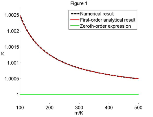
Figure 1: The surface gravity $\kappa$ as a function of the BH “normalized mass” $m/K$. The dashed-dotted black curve displays our numerical results, which were calculated for 250 values of $m/K$ throughout the range $100<m/K<500$. The first-order theoretical prediction $\kappa\cong 1+k/(4m)$ is the solid red curve. These two curves are actually visually indistingwishable. For comparison we also display the corresponding zeroth-order expression $\kappa=1$, the solid green line.

In the analytical derivation above we have imposed the regularity condition $R^{\prime}_{\left(-\infty\right)}=0$ at the horizon. In addition we have worked with the gauge in which $S_{\left(\infty\right)}=x,\,S^{\prime}_{\left(\infty\right)}=1$, in accord with Eq. (22). In a numerical implementation this would mean that we would have to impose boundary conditions at both boundaries of the simulation, $x\to-\infty$ and $x\to\infty$. This is somewhat inconvenient, though it can still be done, e.g. by iterations.

However, to simplify the numerical procedure we have chosen a different approach: We can use a more convenient gauge for the simulation, and then calculate $\kappa$ using the gauge-invariant expression (33). We have chosen the gauge for the simulation to be $S_{\left(-\infty\right)}=x,\,S^{\prime}_{\left(-\infty\right)}=1$ at the horizon, and integrated the ODE system (24,25) from the horizon towards infinity. The boundary conditions for $R$ are taken to be $R^{\prime}_{\left(-\infty\right)}=0$ as well as $R_{\left(-\infty\right)}=m$. In this way all our boundary conditions are specified at $x=-\infty$. In this gauge it easily follows from Eq. (33) that $\kappa=1/S^{\prime}_{\left(\infty\right)}$.

The results of our numerical simulations are presented in Fig. 1. The graph demonstrates an excellent agreement between the numerical solution and our theoretical prediction, based on the first-order analysis. This figure also indicates very clearly that the first-order correction is really needed: The numerical results deviate substatially from the zero-order outflux (the horizontal line $\kappa=1$, which is the infinite-mass limit).

Finally we note that our numerical simulations also reveal a second-order correction term in $\kappa$. This additional term is consistent (within the numerical accuracy) with

$$\frac{3}{32}\left(\frac{K}{m}\right)^{2}.$$

This of course implies a corresponding second-order correction in the Hawking temperature and the outflux.

VI Discussion

We have found analytically, and confirmed numerically, that in a large-mass ($m\gg K$), static, CGHS semiclassical BH the surface gravity $\kappa$ admits a small semiclassical correction $\propto K/m$, presented in Eq. (41). Correspondingly, the Hawking temperature and outflux also get finite-mass corrections, as shown in Eqs. (42,43).

As was already mentioned above, previous analytical Aprox1 as well as numerical APR ; Dori_Ori analyses of the Hawking radiation emitted from an evaporating CGHS BH revealed the presence of a semiclassical correction term $\propto K/m$ in the outflux. Our analysis shows that this correction term is precisely the same (at order $K/m$) in the static and evaporating cases. Namely, Eq. (43) holds in the evaporating case as well (provided that one interprets $m$ as the Bondi mass).

In the evaporating case, one may be tempted to interpret the finite-mass correction to the outflux as an indication for the non-thermal character of the Hawking radiation. Such deviations from thermality might be important for certain aspects of the information puzzle APR . Our analysis of the static case suggests a different interpretation of this $\propto K/m$ correction to the outflux: The backreaction of the renormalized stress-energy tensor $\hat{T}_{\alpha\beta}$ obviously modifies the background geometry, and as a consequence the BH’s surface gravity $\kappa$ is modified too. This inevitably leads to a change in the Hawking temperature, through the standard relation $T_{H}=\kappa/2\pi$ (which should exactly hold, for a static BH, even in the semiclassical case). In turn, this correction in $T_{H}$ naturally leads to a corresponding correction in the outflux, through the standard quadratic relation between temperature and outflux (the 2D analog of the Stefan-Boltzmann law, which states that the outflux should be proportional to the square of the temperature). Indeed, this exact quadratic relation between outflux and Hawking temperature is guaranteed to hold in the 2D semiclassical (static) BHs of the CGHS model, as demonstrated in Eqs. (34) and (35). This relation is also reflected in our explicit first-order results, Eqs. (42) and (43). Thus, in the static case the Hawking outflux remains precisely thermal (despite the semiclassical backreaction), even though the Hawking temperature gets a small semiclassical correction.

Turning now to the evaporating case, since the first-order correction to the outflux precisely agrees with the static result (43), it appears that this $O(K/m)$ correction merely reflects the change in the Hawking temperature due to backreaction (rather than deviations from thermality). Indeed one may anticipate small deviations from thermality in the dynamical, evaporating case; however, such deviations seemingly appear only at second or higher orders in $K/m$.

Appendix A Linear semiclassical correction

We display here the full solution to the linearized semiclassical equations (38,39):

$$\delta R=\frac{K}{4}\left[\ln\left(\frac{e^{x}+m}{m}\right)+\frac{e^{x}}{m}\left(x-\ln(e^{x}+m)\right)\right],$$

$$\delta S=\frac{K}{4m}\left[\frac{m}{e^{x}+m}+x-\ln\left(e^{x}+m\right)\right].$$

The four integration constants were chosen here such that $\delta S$ and $\delta S^{\prime}$ vanish at infinity (in accord with our gauge condition), and $\delta R,\delta R^{\prime}$ vanish at the horizon. [By differentiating the last equation one recovers Eq. (40) for $\delta S^{\prime}$.]

References

- (1) S. W. Hawking, “Particle creation by black holes”, Commun. Math. Phys. 43, 199 (1975).
- (2) C. G. Callan, S. B. Giddings, J. A. Harvey and A. Strominger, “Evanescent black holes”, Phys. Rev. D45, 1005 (1992); arXiv:hep-th/9111056.
- (3) See also A. Ori, “Approximate solution to the CGHS field equations for two-dimensional evaporating black holes”, Phys. Rev. D82, 104009 (2010); arXiv:1007.3856.
- (4) Static CGHS black holes were previously studied in B. Birnir, S. B. Giddings, J. A. Harvey and A. Strominger, “Quantum black holes”, Phys. Rev. D 46, 638 ( 1992); arXiv:hep-th/9203042.
- (5) A. Ori (Unpublished notes); see http://physics.technion.ac.il/~amos/outflux.pdf [see in particular Eq. (141) therein].
- (6) A. Ashtekar, F. Pretorius and F. M. Ramazanoglu, “Surprises in the evaporation of 2-dimensional black holes”, Phys. Rev. Lett. 106, 161303 (2011), arXiv:1011.6442; Phys. Rev. D83, 044040 (2011 ); arXiv:1012.0077.
- (7) L. Dori and A. Ori, “Finite-mass correction to 2D Black-hole evaporation rate”, Phys. Rev. D 85, 124015 (2012); arXiv:1201.6386.
- (8) D. Levanony and A. Ori, “Interior design of a two-dimensional semiclassic black hole”, Phys. Rev. D 80, 084008 (2009); arXiv:0910.2333
- (9) O. B. Zaslavskii, “Entropy of semiclassical 2D dilaton black holes away from the Hawking temperature”, Mod. Phys. Lett. A17, 1775 (2002); arXiv:hep-th/0208206.