Classical and quantum Hořava-Lifshitz cosmology in a minisuperspace perspective

Abstract

We study the classical and quantum models of a Friedmann-Robertson-Walker (FRW) cosmology in the framework of the gravity theory proposed by Hořava, the so-called Hořava-Lifshitz theory of gravity. Beginning with the ADM representation of the action corresponding to this model, we construct the Lagrangian in terms of the minisuperspace variables and show that in comparison with the usual Einstein-Hilbert gravity, there are some correction terms coming from the Hořava theory. Either in the matter free or in the case when the considered universe is filled with a perfect fluid, the exact solutions to the classical field equations are obtained for the flat, closed and open FRW model and some discussions about their possible singularities are presented. We then deal with the quantization of the model in the context of the Wheeler-DeWitt approach of quantum cosmology to find the cosmological wave function. We use the resulting wave functions to investigate the possibility of the avoidance of classical singularities due to quantum effects.
PACS numbers: 04.50.+h, 98.80.Qc, 04.60.Ds
Keywords: Hořava-Lifshitz cosmology, Quantum cosmology

1 Introduction

Since $2009$ when a new theory of gravity was first introduced by Hořava [1], many efforts have been made in this area and the corresponding results have been followed by a number of works, the main motivations of which lie in the results of quantum gravity and cosmology, see for instance [2]. Since this kind of gravitational theory has its roots in the Lifshitz work on the second-order phase transition in solid state physics, it is usually referred to as the Hořava-Lifshitz (HL) theory of gravity. Like another candidates for quantum gravity such as string theory, HL gravity is also a completion of general relativity (GR) at high energy ultraviolet (UV) regime and reduces to standard GR in the low energy infra-red (IR) limit. However, in the framework of the HL theory, the well-known phenomenon of Lorentz symmetry breaking at high energies is described somehow in a different way. Indeed the basic idea behind HL is that the Lorentz symmetry will be broken through a Lifshitz-like process, i.e., through an anisotropic scaling (characterized by a scale parameter $b$ and the dynamical critical exponent $z$) between space and time as

$$t\rightarrow b^{z}t,\hskip 14.22636pt{\bf x}\rightarrow b{\bf x}.$$ (1)

There are theories correspond to the different values of $z$. While for $z=1$ the standard relativistic scale invariance with Lorentz symmetry (the IR limit) is recovered, the UV gravitational theory proposed in [1] requires $z=3$. Because of the asymmetry of space and time in HL theory the most common representation of the space-time metric is its ADM form which in terms of the lapse function $N(t,{\bf x})$, shift vector $N^{a}(t,{\bf x})$ and spacial metric $h_{ab}(t,{\bf x})$ takes the general form

$$g_{\mu\nu}(t,{\bf x})=\left(\begin{array}[]{cc}-N^{2}(t,{\bf x})+N_{a}(t,{\bf x})N^{a}(t,{\bf x})&N_{b}(t,{\bf x})\\ N_{a}(t,{\bf x})&h_{ab}(t,{\bf x})\\ \end{array}\right).$$ (2)

Depending on whether the lapse function is a function only of $t$ or of $(t,{\bf x})$, the theory is called projectable or non-projectable. As pointed out in [1], since in cosmological metrics the lapse function labels the time parameter, it is quite reasonable to choose it as a projectable function. However, more general cases in which the lapse function is taken as a non-projectable function are studied in [3]. Indeed, in these references the authors have examined some consistency conditions present in the projectable HL theory and its non-projectable extension. They found that while the projectable theory suffers from the presence of the ghost mode and hence cannot be consistent, the non-projectable models are free from such ghost instabilities. As a remark we would like to to emphasize that this problem cannot be seen in the minisuperspace approximation of cosmological models in which we restrict the metric and the matter fields to be homogeneous. Therefore, the study of the minisuperspace cosmology in the framework of projectable HL gravity is quite reasonable. However, one should bear in mind that even at the classical level the above mentioned instability could be visible when the the perturbations analysis about homogeneous background is performed. There is yet another issue related to the HL theory, the so called detailed balance condition. The gravitational action of the model consists of the kinetic part ${\cal S}_{K}$ and the potential part ${\cal S}_{V}$ as ${\cal S}={\cal S}_{K}+{\cal S}_{V}$. The kinetic part comes from the Einstein-Hilbert action usually written in terms of the ADM variables (see the relation (2) bellow). For the potential part the following general form is proposed in [1]

$${\cal S}_{V}=\int d^{4}x\sqrt{-g}V[h_{ab}],$$ (3)

where $V$ is a scalar function which depends only on the spacial metric $h_{ab}$ and its spacial derivatives. Taking a three dimensional HL model with $z=3$, this function may be constructed by a superposition of the quadratic (in curvature) terms such as

$$\nabla_{a}R_{bc}\nabla^{a}R^{bc},\hskip 14.22636pt\nabla_{a}R_{bc}\nabla^{b}R^{ca},\hskip 14.22636ptR\nabla^{2}R,\hskip 14.22636ptR^{ab}\nabla^{2}R_{ab},$$ (4)

and cubic terms such as

$$R^{3},\hskip 14.22636ptR^{a}_{b}R^{b}_{c}R^{c}_{a},\hskip 14.22636ptRR_{ab}R^{ab}.$$ (5)

Among the very different possible combinations, Hořava considered a special form, known as ”detailed balance condition” satisfying model as

$${\cal S}_{V}\sim\int d^{4}x\sqrt{-g}E^{ab}{\cal G}_{abcd}E^{cd},$$ (6)

where ${\cal G}_{abcd}$ is the DeWitt metric and $E^{ab}$ is a tensor constructed by variation of some function $W[h_{ab}]$ with respect to the spacial metric. By choosing a suitable ansatz for the function $W$, he then showed that in a $z=3$ theory with detailed balance condition the potential is a combination of the terms (see [1] for details)

$$\nabla_{a}R_{bc}\nabla^{a}R^{bc},\hskip 14.22636pt\nabla_{a}R_{bc}\nabla^{b}R^{ac},\hskip 14.22636pt\nabla_{a}R\nabla^{a}R.$$ (7)

The issue of the detailed balance condition makes the theory to have simpler renormalization properties. Although the detailed balanced system exhibit simpler quantum behavior, it is shown in [4] that if one relaxes it, the resulting Lagrangian with extra allowed terms is well-behavior enough to recover the model with detailed balance.

In this paper we shall consider a FRW cosmological model in the framework of a projectable HL gravity without detailed balance condition. Our approach to deal with such a problem is through its representation with minisuperspace variables. Minisuperspace formulation of HL cosmology is studied in some works, see for instance [5]-[7], to obtain its possible classical and quantum solutions. Here, we first consider the vacuum case in which the cosmological model is free from the presence of any kind of matter fields and see that the corresponding classical solutions exhibit some types of singularities. We then will add a perfect fluid as the matter into the model and obtain some exact solutions in the cases of flat, closed and open FRW cosmologies. Since our aim in the quantum part of the model is to investigate the time evolution of the wave function, we prefer to use the perfect fluid in its Schutz formalism in which the Hamiltonian of the fluid consists of a linear momentum, the variable canonically conjugate to which may play the role of a time parameter. In both vacuum and perfect fluid cases, we construct the corresponding quantum cosmology based on the canonical approach of Wheeler-DeWitt theory to see how things may change their behavior if the quantum mechanical considerations come into the model.

2 The model

In this section we start by the FRW cosmology within the framework of HL gravity. In a quasi-spherical polar coordinate the metric of space time is assumed to be

$$ds^{2}=-N^{2}(t)dt^{2}+a^{2}(t)\left[\frac{dr^{2}}{1-kr^{2}}+r^{2}\left(d\vartheta^{2}+\sin^{2}\vartheta d\varphi\right)\right],$$ (8)

where $N(t)$ is the lapse function, $a(t)$ the scale factor and $k=1$, $0$ and $-1$ corresponds to the closed, flat and open universe respectively. It is clear that in terms of the ADM variables the above metric can be written as

$$ds^{2}=-N^{2}(t)dt^{2}+h_{ab}dx^{a}dx^{b},$$ (9)

in which

$$h_{ab}=a^{2}(t)\mbox{diag}\left(\frac{1}{1-kr^{2}},r^{2},r^{2}\sin^{2}\vartheta\right),$$

is the intrinsic metric induced on the spatial $3$-dimensional hypersurfaces. The action of the model consists of the gravitational part ${\cal S}_{g}$ and the matter action ${\cal S}_{m}$ as

$${\cal S}={\cal S}_{g}+{\cal S}_{m}.$$ (10)

The matter part of the action is independent of the HL corrections to the gravity part. In the context of the ADM formalism, following [4] and with the same notation as is used in [5, 6], the projectable HL gravity without detailed balance has the (gravitational) action (in what follows we work in units where $c=\hbar=1$)

$${\cal S}_{g}=\frac{M_{Pl}^{2}}{2}\int_{{\cal M}}d^{3}xdtN\sqrt{h}\left[K_{ab}K^{ab}-\lambda K^{2}-g_{0}M_{Pl}^{2}-g_{1}R-M_{Pl}^{-2}\left(g_{2}R^{2}+g_{3}R_{ab}R^{ab}\right)\right.$$

$$\left.-M_{Pl}^{-4}\left(g_{4}R^{3}+g_{5}RR^{a}_{b}R^{b}_{a}+g_{6}R^{a}_{b}R^{b}_{c}R^{c}_{a}+g_{7}R\nabla^{2}R+g_{8}\nabla_{a}R_{bc}\nabla^{a}R^{bc}\right)\right]+M_{Pl}^{2}\int_{\partial{\cal M}}d^{3}x\sqrt{h}K,$$ (11)

where $M_{Pl}=(8\pi G)^{-1/2}$ is the Planck mass, $K_{ab}$ are the components of the extrinsic curvature tensor which describes how much the spatial space $h_{ab}$ (which is the boundary $\partial{\cal M}$ of the four-dimensional manifold ${\cal M}$) is curved in the way it sits in the space time manifold. Also, $h$ and $R$ are the determinant and Ricci scalar of the spatial geometry $h_{ab}$ respectively, and $K$ represents the trace of $K_{ab}$. The constants $\lambda$ and $g_{i}$ ($i=0,1,...,8$) denote the HL corrections to the usual GR. In comparison with the ADM representation of GR action, that is

$${\cal S}_{g}=\frac{M_{Pl}^{2}}{2}\left[\int_{{\cal M}}d^{3}xdtN\sqrt{h}\left(K_{ab}K^{ab}-K^{2}+R-2\Lambda\right)+2\int_{\partial{\cal M}}d^{3}x\sqrt{h}K\right],$$

we conclude that the consensus GR is recovered if one sets the cosmological constant as $\Lambda=g_{0}M_{Pl}^{2}/2$, $g_{1}=-1$ and $\lambda=1$. However, as is mentioned in [5], we take $\lambda$ as a running constant which represents the IR limit of the gravitational theory. With these identifications, the action (2) may be rewritten as

$${\cal S}_{g}=\frac{M_{Pl}^{2}}{2}\int_{{\cal M}}d^{3}xdtN\sqrt{h}\left[K_{ab}K^{ab}-\lambda K^{2}+R-2\Lambda-M_{Pl}^{-2}\left(g_{2}R^{2}+g_{3}R_{ab}R^{ab}\right)\right.$$

$$\left.-M_{Pl}^{-4}\left(g_{4}R^{3}+g_{5}RR^{a}_{b}R^{b}_{a}+g_{6}R^{a}_{b}R^{b}_{c}R^{c}_{a}+g_{7}R\nabla^{2}R+g_{8}\nabla_{a}R_{bc}\nabla^{a}R^{bc}\right)\right]+M_{Pl}^{2}\int_{\partial{\cal M}}d^{3}x\sqrt{h}K.$$ (12)

From its standard definition, the extrinsic curvature is given by

$$K_{ab}=\frac{1}{2N}\left(N_{a|b}+N_{b|a}-\frac{\partial h_{ab}}{\partial t}\right),$$ (13)

where $N_{a}$ is the shift vector and $N_{a|b}$ represents the covariant derivative with respect to $h_{ab}$. Since the shift vector is absent in the FRW models, a simple calculation based on the above definition results in $K_{ab}K^{ab}=\frac{3\dot{a}^{2}}{N^{2}a^{2}}$ and $K=-\frac{3\dot{a}}{Na}$, where a dot represents differentiation with respect to $t$. Also, the Ricci tensor and the Ricci scalar correspond to the $3$-geometry $h_{ab}$ can be obtained as $R_{ab}=\frac{2kh_{ab}}{a^{2}}$ and $R=\frac{6k}{a^{2}}$. The gravitational part for FRW model may now be written by substituting the above results into action (2), giving

$${\cal S}_{g}=\frac{3V_{0}M_{Pl}^{2}(3\lambda-1)}{2}\int dtN\left\{-\frac{a\dot{a}^{2}}{N^{2}}+\frac{6ka}{3(3\lambda-1)}-\frac{2\Lambda a^{3}}{3(3\lambda-1)}-M_{pl}^{-2}\left[\frac{12k^{2}(3g_{2}+g_{3})}{3a(3\lambda-1)}\right]\right.$$

$$\left.-M_{Pl}^{-4}\left[\frac{24k(9g_{4}+3g_{5}+g_{6})}{3a^{3}(3\lambda-1)}\right]\right\},$$ (14)

where $V_{0}=\int d^{3}x\sqrt{h}$ is the integral over spatial dimensions. If we set $\frac{3V_{0}M_{Pl}^{2}(3\lambda-1)}{2}=1$, then we are led to the point-like Lagrangian

$${\cal L}_{g}=N\left(-\frac{a\dot{a}^{2}}{N^{2}}+g_{c}ka-g_{\Lambda}a^{3}-\frac{g_{r}k^{2}}{a}-\frac{g_{s}k}{a^{3}}\right),$$ (15)

where its coefficients are defined as [8]

$$g_{c}=\frac{2}{3\lambda-1},\hskip 14.22636ptg_{\Lambda}=\frac{2\Lambda}{3(3\lambda-1)},\hskip 14.22636ptg_{r}=6V_{0}(3g_{2}+g_{3}),\hskip 14.22636ptg_{s}=18V_{0}^{2}(3\lambda-1)(9g_{4}+3g_{5}+g_{6}).$$ (16)

Now, the gravitational part of the Hamiltonian for this model can be obtained from its standard definition $H_{g}=\dot{a}P_{a}-{\cal L}_{g}$. Noting that

$$P_{a}=\frac{\partial{\cal L}_{g}}{\partial\dot{a}}=-2\frac{a\dot{a}}{N},$$ (17)

one gets

$$H_{g}=N{\cal H}_{g}=N\left[-\frac{P_{a}^{2}}{4a}-g_{c}ka+g_{\Lambda}a^{3}+\frac{g_{r}k^{2}}{a}+\frac{g_{s}k}{a^{3}}\right].$$ (18)

We see that the lapse function enters in the Hamiltonian as a Lagrange multiplier, as expected. Thus, when we vary the Hamiltonian with respect to $N$, we get ${\cal H}_{g}=0$, which is called the Hamiltonian constraint. On the classical level this constraint is equivalent to the Friedmann equation, while on the quantum level, the operator version of this constraint annihilates the wave function of the corresponding universe, leading to the so-called Wheeler-DeWitt equation. Now, let us deal with the matter field with which the action of the model is augmented. As we have mentioned, the matter part of the action is independent of modifications due to the HL terms. Therefore, the matter may come into play in a common way and the total Hamiltonian can be made by adding the matter Hamiltonian to the gravitational part (18). To do this, we consider a perfect fluid whose pressure $p$ is linked to its energy density $\rho$ by the equation of state

$$p=\omega\rho,$$ (19)

where $-1\leq\omega\leq 1$ is the equation of state parameter. According to Schutz’s representation for the perfect fluid [9], its Hamiltonian can be viewed as (see [10] for details)

$$H_{m}=N\frac{P_{T}}{a^{3\omega}},$$ (20)

where $T$ is a dynamical variable related to the thermodynamical parameters of the perfect fluid and $P_{T}$ is its conjugate momentum. Finally, we are in a position in which can write the total Hamiltonian $H=H_{g}+H_{m}$ as

$$H=N{\cal H}_{g}=N\left[-\frac{P_{a}^{2}}{4a}-g_{c}ka+g_{\Lambda}a^{3}+\frac{g_{r}k^{2}}{a}+\frac{g_{s}k}{a^{3}}+\frac{P_{T}}{a^{3\omega}}\right].$$ (21)

The setup for constructing the phase space and writing the Lagrangian and Hamiltonian of the model is now complete. In the following sections, we shall deal with classical and quantum cosmologies which can be extracted from a theory with the above mentioned Hamiltonian.

3 Cosmological dynamics without matter

3.1 Classical model

When the model is free of the contribution of any kind of matter fields, the dynamics is described by Hamiltonian (18). Therefore, the classical equations of motion is governed by the Hamiltonian equations. Equivalently, we can use the constraint equation ${\cal H}=0$ which is nothing but the variation the action with respect to $N$. In this sense, from (17) and (18) we obtain

$$a\dot{a}^{2}+g_{c}ka-g_{\Lambda}a^{3}-\frac{g_{r}k^{2}}{a}-\frac{g_{s}k}{a^{3}}=0.$$ (22)

For the flat case $k=0$, there is no difference between the HL cosmology and the usual FRW model except that the cosmological constant shifts as $\Lambda\rightarrow 3g_{\Lambda}=\frac{2\Lambda}{3\lambda-1}$. In this case the above equation admits the following solutions

$$a(t)=a_{0}e^{\pm\sqrt{g_{\Lambda}}t},$$ (23)

where $a_{0}$ is an integration constant and the positive (negative) sign in the power of the exponential function corresponds to the expansion (contraction) universe. Thus, in this case we have two distinct branches of solutions, one of which begins with zero size at $t=-\infty$ and expands forever according to an exponential de Sitter law, while another has an opposite behavior, i.e., decreases its size from the large values at $t=-\infty$ and tends exponentially to zero as $t\rightarrow\infty$. The situation of the dynamical behavior of the scale factor in this case is shown in figure 1.

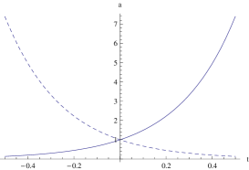
Figure 1: Qualitative behavior of the scale factor for the flat universe. Solid and dashed lines denote the relation (23) for positive and negative signs respectively.

For $k\neq 0$, equation (22) does not seem to have analytical solutions. So we consider the behavior of its solutions only for some limiting cases. When the scale factor is very small, we keep the two last terms in (22) and rewrite it as

$$a\dot{a}^{2}-\frac{g_{r}k^{2}}{a}-\frac{g_{s}k}{a^{3}}=0,$$ (24)

from which we obtain the following implicit relation between $t$ and $a$

$$\frac{a\sqrt{g_{r}a^{2}+kg_{s}}}{2g_{r}}-\frac{kg_{s}\ln\left(g_{r}a+\sqrt{g_{r}^{2}a^{2}+kg_{s}}\right)}{2g_{r}^{3/2}}=\pm t-t_{0},$$ (25)

where $t_{0}$ is an integration constant. In figure 2, we have plotted the scale factor versus time based on the above relation.

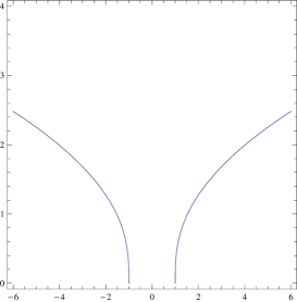
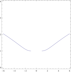
Figure 2: The figures show the evolutionary behavior of the non-flat universe in the early times based on (25). The left and right figures correspond to the $k=1$ and $k=-1$ respectively.

On the other hand, for the late time of cosmic evolution which the scale factor is expected to be large the terms with coefficients $g_{c}$ and $g_{\Lambda}$ in (22) become more important. In such a case we write this equation as

$$\dot{a}^{2}+g_{c}k-g_{\Lambda}a^{2}=0.$$ (26)

For $k=+1$, this equation has two sets of solutions as

$$a_{I}(t)=\frac{1}{2g_{\Lambda}}\left[e^{\sqrt{g_{\Lambda}}(t+t_{0})}+g_{c}g_{\Lambda}e^{-\sqrt{g_{\Lambda}}(t+t_{0})}\right],$$ (27)

and

$$a_{II}(t)=\frac{1}{2g_{\Lambda}}\left[e^{-\sqrt{g_{\Lambda}}(t-t_{0})}+g_{c}g_{\Lambda}e^{\sqrt{g_{\Lambda}}(t-t_{0})}\right],$$ (28)

where $t_{0}$ is an integration constant. Each of these solutions consists of two branches. In one branch the universe contracts and when reaches a minimum size undergoes to an expansion period. Therefore, in the case of of a closed universe we have bouncing cosmologies in which the bounce occurs at $t=-[t_{0}+\frac{1}{2\sqrt{g_{\Lambda}}}\ln(\frac{1}{g_{c}g_{\Lambda}})]$ for $a_{I}(t)$ and at $t=[t_{0}-\frac{1}{2\sqrt{g_{\Lambda}}}\ln(g_{c}g_{\Lambda})]$ for $a_{II}(t)$. On the other hand, for $k=-1$ the solutions to the equation (26) take the form

$$a(t)=\left\{\begin{array}[]{ll}a^{I}(t)=\frac{1}{2g_{\Lambda}}\left[e^{-\sqrt{g_{\Lambda}}(t-t_{0})}-g_{c}g_{\Lambda}e^{\sqrt{g_{\Lambda}}(t-t_{0})}\right],\hskip 14.22636ptt<t_{0}-\frac{1}{\sqrt{2g_{\Lambda}}}\ln(g_{c}g_{\Lambda}),\\ \\ a^{II}(t)=\frac{1}{2g_{\Lambda}}\left[e^{\sqrt{g_{\Lambda}}(t+t_{0})}-g_{c}g_{\Lambda}e^{-\sqrt{g_{\Lambda}}(t+t_{0})}\right],\hskip 14.22636ptt>-t_{0}+\frac{1}{\sqrt{2g_{\Lambda}}}\ln(g_{c}g_{\Lambda}).\end{array}\right.$$ (32)

We see that in the time interval $t<t_{0}-\frac{1}{\sqrt{2g_{\Lambda}}}\ln(g_{c}g_{\Lambda})$ the scale factor decrease and tends its evolution at $t_{0}-\frac{1}{\sqrt{2g_{\Lambda}}}\ln(g_{c}g_{\Lambda})$ with zero size. Also, for $t>-t_{0}+\frac{1}{\sqrt{2g_{\Lambda}}}\ln(g_{c}g_{\Lambda})$, the universe has an expanding behavior begins its evolution with a zero size singularity at $-t_{0}+\frac{1}{\sqrt{2g_{\Lambda}}}\ln(g_{c}g_{\Lambda})$. These two branches of solutions are separated from each other by a classically forbidden region corresponding to the time interval $t_{0}-\frac{1}{\sqrt{2g_{\Lambda}}}\ln(g_{c}g_{\Lambda})<t<-t_{0}+\frac{1}{\sqrt{2g_{\Lambda}}}\ln(g_{c}g_{\Lambda})$ for which no open classical solutions exist. The above results are summarized in figure 3.

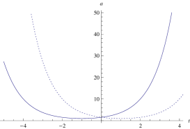
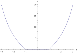
Figure 3: Left: Late time behavior of the non-flat universe for $k=1$. Right: The same figure for $k=-1$.

3.2 Quantum model

Now, we shall study the quantum behavior of the model described by the Hamiltonian (18). One way to do such a study is to investigate the well-known Wheeler-DeWitt equation for the corresponding universe, that is

$$\left[\frac{1}{a}\frac{d^{2}}{da^{2}}-\frac{p}{a^{2}}\frac{d}{da}+4\left(-g_{c}ka+g_{\Lambda}a^{3}+\frac{g_{r}k^{2}}{a}+\frac{g_{s}k}{a^{3}}\right)\right]\Psi(a)=0,$$ (33)

where $\Psi(a)$ is the wave function corresponds to the quantum universe and the parameter $p$ represents the ambiguity in the ordering of factors $a$ and $P_{a}$ in the first term of (18). In the case of a flat universe $k=0$, to see the correspondence of the classical and quantum solutions, we note that for large values of scale factor, the behavior of the system can be obtained in the WKB (semiclassical) approximation. Then substituting $\Psi(a)=\Omega(a)e^{iS(a)}$ in equation (33) leads to the modified Hamilton-Jacobi equation

$$-\frac{1}{4a}\left(\frac{ds}{da}\right)^{2}+g_{\Lambda}a^{3}+{\cal Q}(a)={\cal H}\left(a,P_{a}=\frac{dS}{da}\right)+{\cal Q}(a)=0,$$ (34)

in which the quantum potential is defined as ${\cal Q}(a)=\frac{1}{4a\Omega}\frac{d^{2}\Omega}{da^{2}}-\frac{1}{a^{2}\Omega}\frac{d\Omega}{da}$. It is well known that the quantum effects are important for small values of the scale factor and in the limit of the large scale factor can be neglected. Therefore, in the semiclassical approximation region we can omit the ${\cal Q}$ term in equation (34) and obtain the phase function $S(a)$ as $S(a)=\pm\frac{2}{3}\sqrt{g_{\Lambda}}a^{3}$. In the WKB method, the correlation between classical and quantum solutions is given by the relation $P_{a}=\frac{\partial S}{\partial a}$. Thus, using the definition of $P_{a}$ in (17), the equation for the classical trajectories becomes $a(t)=a_{0}e^{\pm\sqrt{g_{\Lambda}}t}$, which shows that the classical cosmology of equation (23) is exactly recovered. The meaning of this result is that for large values of the scale factor, the effective action corresponding to the expanding and contracting universes is very large and the universe can be described classically. On the other hand, for small values of the scale factor we cannot neglect the quantum effects and the classical description breaks down. Since the WKB approximation is no longer valid in this regime, one should go beyond the semiclassical approximation. For the flat FRW metric we have $k=0$ and the two linearly independent solutions to equation (33) can be expressed in terms of the Bessel functions $J_{\nu}(x)$ leading to the following general solution

$$\Psi(a)=a\left[c_{1}J_{1/3}\left(\frac{2}{3}\sqrt{g_{\Lambda}}a^{3}\right)+c_{2}J_{-1/3}\left(\frac{2}{3}\sqrt{g_{\Lambda}}a^{3}\right)\right],$$ (35)

where $c_{1,2}$ are integration constants. To find the above solutions we have noted that the factor-ordering parameter $p$ does not affect the semiclassical probabilities [11], and so we have chosen $p=1$ to make the differential operator appearing in the Wheeler-DeWitt equation the Laplacian operator of the minisupermetric (see [12]). With an eye to the classical solutions (23), it is clear that the model is free of classical Big-Bang singularity in which $a(t_{0})=0$ for some $t_{0}$. Therefore, we expect that the quantum model predicts a zero probability for the creation of the universe with zero size. This fact lead us to impose the boundary condition $\Psi(a=0)=0$ on the wave function, which results in $c_{2}=0$. Note that equation (33) is a Schrödinger-like equation for a fictitious particle with zero energy moving in the field of the superpotential $U(a)=-4g_{\Lambda}a^{4}$. Usually, in the presence of such a potential, the mini-superspace can be divided into two regions, $U>0$ and $U<0$, which could be termed the classically forbidden and classically allowed regions, respectively. In the classically forbidden region the behavior of the wave function is exponential, while in the classically allowed region the wave function behaves oscillatorily. In the quantum tunneling approach [11], the wave function is so constructed as to create a universe emerging from nothing by a tunneling procedure through a potential barrier in the sense of usual quantum mechanics. Now, in our model, the superpotential is always negative, which means that there is no possibility of tunneling anymore, since a zero energy system is always above the superpotential. In such a case, tunneling is no longer required, as classical evolution is possible. As a consequence, the wave function always exhibits oscillatory behavior. In figure 4, we have plotted the square of the wave functions for typical values of the parameters . It is seen from this figure that the wave function has a well-defined behavior near $a=0$ and describes a universe emerging out of nothing without any tunneling. Now to see that how the quantum solutions may describe an expanding or contracting universe, we use a mechanism which we have called the probabilistic evolutionary process (PEP), based on the probabilistic structure of quantum systems, to provide a sense of the evolution embedded in the wave function of the universe (see [14] for details). This is based on the fact that in quantum systems the square of a state defines the probability, ${\cal P}_{a}=|\Psi(a)|^{2}$. To make the discussion more clear, let us take a specific initial condition corresponding to the point $P$. Then, PEP states that the system (here specified by the scale factor $a$) moves continuously to a state with higher probability and thus $P$ moves to the right to reach the point $Q$, a local maximum. Therefore, the (expanding) universe begins its evolution by a monotonically increasing scale factor to reach the point $Q$. In this sense the transition $R\rightarrow Q$ describes a contracting universe. On the other hand, the emergence of several peaks in the wave function may be interpreted as a representation of different quantum states that may communicate with each other through tunneling. This means that there are different possible universes (states) from which the present universe could have evolved and tunneled in the past, from one universe (state) to another. Based on this interpretation, one can argue that from the states located on the larger peaks of the wave function a tunneling may occurs to reach the states located on the smaller peaks and then the universe evolved according to PEP. We schematically show such procedures as

$$\mbox{expanding universe}:P{\buildrel{PEP}\over{\longrightarrow}}Q{\buildrel{tunnel.}\over{\longrightarrow}}T{\buildrel{PEP}\over{\longrightarrow}}U...$$ (36)

As the scale factor grows the probabilities become small and smaller and the universe undergoes its classical region. For the contraction universe similar discussion as above would be applicable as well.

Figure 4: Qualitative behavior of the probability ($=|\Psi(a)|^{2}$) versus scale factor for the flat empty universe, see relation (35).

Now, let us to deal with the Wheeler-DeWitt equation (33) in the case of $k\neq 0$. Like the classical solutions in this case, we analyze the quantum solutions in the limiting cases of small and large scale factor. For the very small values for the scale factor the terms with coefficients $g_{c}$ and $g_{\Lambda}$ are negligible in comparison with the terms with HL parameters $g_{r}$ and $g_{s}$. In this limit the solutions to the equation (33) read as

$$\Psi(a)=a\left[c_{1}J_{\sqrt{1-4kg_{s}}}\left(2k\sqrt{g_{r}}a\right)+c_{2}Y_{\sqrt{1-4kg_{s}}}\left(2k\sqrt{g_{r}}a\right)\right].$$ (37)

Since the behavior of the Bessel functions for the small argument is $J_{\nu}(z)\sim z^{\nu}+O(z^{\nu+2})$ and $Y_{\nu}(z)\sim z^{-\nu}+O(\frac{1}{z^{\nu(\nu-2)}})$, we set $c_{2}=0$ and simplify the above relation for small $a$ as

$$\Psi(a)\sim a^{1+\sqrt{1-4kg_{s}}}.$$ (38)

The probability of creation an universe with scale factor $a$ is

$$|\Psi(a)|^{2}\sim\left\{\begin{array}[]{ll}a^{2},\hskip 14.22636pt1-4kg_{s}<0,\\ \\ a^{2+2\sqrt{1-4kg_{s}}},\hskip 14.22636pt1-4kg_{s}>0,\end{array}\right.$$ (42)

which in both cases describes an expanding non-singular behavior in the early times of cosmic evolution in agreement with the classical solutions presented in figure 2.

For the large scale factor, a WKB analysis like we have done for the flat case yields the classical solutions (27)-(32), which shows that our treatment for quantization of the model lies in a right way. However, for $a>>1$ we can neglect the last two terms with coefficients $g_{r}$ and $g_{s}$ in (33) and write its solutions in terms of the Airy functions as

$$\Psi(a)=c_{1}\mbox{Ai}\left(\frac{kg_{c}-g_{\Lambda}a^{2}}{g_{\Lambda}^{2/3}}\right)+c_{2}\mbox{Bi}\left(\frac{kg_{c}-g_{\Lambda}a^{2}}{g_{\Lambda}^{2/3}}\right).$$ (43)

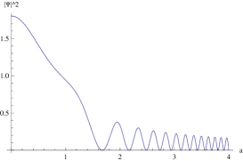
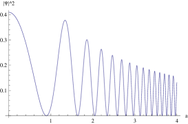
Figure 5: Left: Late square of the wave function (43) for $k=1$. Right: The same figure for $k=-1$.

A glance at the shape of this wave function which is qualitatively plotted in figure 5 for typical values of the parameters, shows that it has a damping oscillatory behavior denoting a classically allowed region. Such a wave function is also found in [15] to describe the dynamical behavior of a universe dominated by the cosmological constant.

4 Cosmological dynamics with perfect fluid

4.1 Classical model

Now, we assume that a perfect fluid in its Schutz’s representation is coupled with gravity. In this case the Hamiltonian (21) describes the dynamics of the system. The advantage of using Schutz formalism is that, in a natural way, it can offer a time parameter in terms of dynamical variables of the perfect fluid. Indeed, the equations of motion for $T$ and $P_{T}$ read as

$$\dot{T}=\left\{T,H\right\}=\frac{N}{a^{3\omega}},\hskip 14.22636pt\dot{P_{T}}=\left\{P_{T},H\right\}=0.$$ (44)

A glance at the above equations shows that with choosing the gauge $N=a^{3\omega}$, we shall have

$$N=a^{3\omega}\Rightarrow T=t,$$ (45)

which means that variable $T$ may play the role of time in the model. Therefore, the Friedmann equation $H=0$ can be written in the gauge $N=a^{3\omega}$ as follows

$$\dot{a}^{2}=-g_{c}ka^{6\omega}+g_{\Lambda}a^{6\omega+2}+g_{r}k^{2}a^{6\omega-2}+g_{s}ka^{6\omega-4}+P_{0}a^{3\omega-1},$$ (46)

where we take $P_{T}=P_{0}=\mbox{const}.$ from the second equation of equation (44). Like the previous section, let us deal first with the solutions of this equation for the flat background, $k=0$. In this case, the solutions can be represented by

$$\frac{2a^{\frac{3-3\omega}{2}}}{3\sqrt{P_{0}}(1-\omega)}\hskip 11.38092ptF_{12}\hskip 11.38092pt\left(\frac{1-\omega}{2+2\omega},\frac{1}{2},\frac{3+\omega}{2+2\omega};-\frac{g_{\Lambda}}{P_{0}}a^{3+3\omega}\right)=\pm t-t_{0},$$ (47)

for $\omega\neq 1$ (for $\omega=1$, there are no real solutions), where $F_{12}\hskip 11.38092pt(a,b,c;z)$ is hypergeometric function and $t_{0}$ is a constant of integration. In figure 6 we have plotted the scale factor versus time for several values of $\omega$. As is clear from the figures the resulting cosmology is consisted of two contraction and expansion branches which are separated from each other by a classically forbidden region in which there are no physically acceptable solutions.

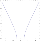
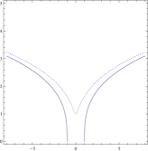
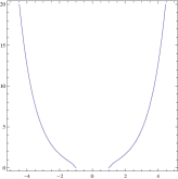
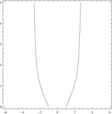
Figure 6: Qualitative behavior of the scale factor versus time based on relation (47) with numerical values $P_{0}=1$, $g_{\Lambda}=1$ and $t_{0}=1$ for the parameters. The figures are plotted for $\omega=-1/3,-1,0,1/3$ from left to right. The dashed line in the figure corresponding to the case $\omega=-1$ shows the expectation value of the scale factor, see (70).

For $k\neq 0$, it is better to deal with the equation (46) in some special cases. To this end, we shall choose typical values for the equation of state parameter $\omega$ as follows.

$\bullet$ $\omega=-1/3$, for which equation (46) reads

$$\dot{a}^{2}=-g_{c}ka^{-2}+g_{\Lambda}+g_{r}k^{2}a^{-4}+g_{s}ka^{-6}+P_{0}a^{-2}.$$ (48)

In the region where the scale factor is small, i.e., in the early times, we can keep only the terms with coefficients $g_{r}$ and $g_{s}$ on the right hand side of the above equation which results the following solution

$$\frac{(kg_{r}a^{2}-2g_{s})\sqrt{g_{r}a^{2}+kg_{s}}}{2kg_{r}^{2}}=\pm t-t_{0}.$$ (49)

For large scale factors, on the other hand, the other terms become more important and one obtains the late time behavior as

$$a(t)=\left[g_{\Lambda}^{2}(\pm t-t_{0})^{2}-(P_{0}-g_{c}k)\right]^{1/2}.$$ (50)

$\bullet$ $\omega=1/3$, for which equation (46) takes the form

$$\dot{a}^{2}=-g_{c}ka^{2}+g_{\Lambda}a^{4}+g_{s}ka^{-2}+P_{0}+g_{r}k^{2},$$ (51)

which has the solutions

$$a(t)=\left(\pm\sqrt{g_{s}k}t-t_{0}\right)^{1/2},$$ (52)

for the early times, and

$$a(t)=\left(\pm t-t_{0}\right)^{-1},$$ (53)

for late times of cosmic evolution. A quick look at these solutions shows that all of them have some kinds of singularities. In the next subsection we will deal with the quantization of this model to see how things change according to the quantum picture of the corresponding cosmology.

4.2 Quantum model

Now, let us to investigate how the above picture may be modified if one deals with the quantization of the model described by the Hamiltonian (21). The Wheeler-DeWitt equation corresponding to this Hamiltonian reads

$$\left[a^{-1}\frac{\partial^{2}}{\partial a^{2}}-a^{-2}\frac{\partial}{\partial a}-4ia^{-3\omega}\frac{\partial}{\partial T}+4\left(-g_{c}ka+g_{\Lambda}a^{3}+\frac{g_{r}k^{2}}{a}+\frac{g_{s}k}{a^{3}}\right)\right]\Psi(a,T)=0,$$ (54)

in which we have taken the factor ordering parameter $p=1$ as before. Separation the variables in the above equation in the form

$$\Psi(a,T)=e^{iET}\psi(a),$$ (55)

yields

$$\left[a^{2}\frac{d^{2}}{da^{2}}-a\frac{d}{da}+4\left(-g_{c}ka^{4}+g_{\Lambda}a^{6}+g_{r}k^{2}a^{2}+g_{s}k+Ea^{3-3\omega}\right)\right]\psi(a)=0.$$ (56)

If $k=0$, the above equation has exact solutions for some special values of $\omega$ as

$$\psi_{E}(a)=\left\{\begin{array}[]{ll}c_{1}\mbox{Ai}\left(-\frac{E+g_{\Lambda}a^{2}}{g_{\Lambda}^{2/3}}\right)+c_{2}\mbox{Bi}\left(-\frac{E+g_{\Lambda}a^{2}}{g_{\Lambda}^{2/3}}\right),\hskip 14.22636pt\omega=-1/3,\\ \\ a\left[c_{1}J_{1/3}\left(\frac{2}{3}\sqrt{E+g_{\Lambda}}a^{3}\right)+c_{2}J_{-1/3}\left(\frac{2}{3}\sqrt{E+g_{\Lambda}}a^{3}\right)\right],\hskip 14.22636pt\omega=-1,\\ \\ a^{2}e^{-\frac{2}{3}i\sqrt{g_{\Lambda}}a^{3}}\left[c_{1}M\left(\frac{5\sqrt{g_{\Lambda}}+2iE}{6\sqrt{g_{\Lambda}}},\frac{5}{3};\frac{4}{3}i\sqrt{g_{\Lambda}}a^{3}\right)+c_{2}U\left(\frac{5\sqrt{g_{\Lambda}}+2iE}{6\sqrt{g_{\Lambda}}},\frac{5}{3};\frac{4}{3}i\sqrt{g_{\Lambda}}a^{3}\right)\right],\hskip 14.22636pt\omega=0,\end{array}\right.$$ (62)

where $M(a,b;z)$ and $U(a,b;z)$ are confluent hypergeometric functions. Now the eigenfunctions of the Wheeler-DeWitt equation can be written as

$$\Psi_{E}(a,T)=e^{iET}\psi_{E}(a).$$ (63)

We may now write the general solution to the Wheeler-DeWitt equation as a superposition of its eigenfunctions; that is,

$$\Psi(a,T)=\int_{0}^{\infty}A(E)\Psi_{E}(a,T)dE,$$ (64)

where $A(E)$ is a suitable weight function to construct the wave packets. Since the above relations seem to be too complicated to extract an analytical expression for the wave function, let us focus our attention on the case $\omega=-1$ for which analytical expression for the integral (64) is found if we choose the function $A(E)$ to be a quasi-Gaussian weight factor. To end this, we take $c_{2}=0$ to satisfy the boundary condition $\psi_{E}(a=0)=0$ and write down the wave function as

$$\Psi(a,T)=\int_{0}^{\infty}aA({\cal E})e^{-ig_{\Lambda}T}e^{i{\cal E}T}J_{1/3}\left(\frac{2}{3}\sqrt{{\cal E}}a^{3}\right)d{\cal E},$$ (65)

where ${\cal E}=E+g_{\Lambda}$. Now, by using the equality

$$\int_{0}^{\infty}e^{-\alpha z^{2}}z^{\nu+1}J_{\nu}(\beta z)dz=\frac{\beta^{\nu}}{(2\alpha)^{\nu+1}}e^{-\frac{\beta^{2}}{4\alpha}},$$ (66)

we choose the weight function as $A({\cal E})={\cal E}^{1/6}e^{-\gamma{\cal E}}$, to obtain

$$\Psi(a,T)={\cal N}e^{-ig_{\Lambda}T}\frac{a^{2}}{(\gamma-iT)^{4/3}}\exp\left(-\frac{1}{9}\frac{a^{6}}{\gamma-iT}\right),$$ (67)

where ${\cal N}$ is a numerical factor and $\gamma$ is an arbitrary positive constant. Now, having the above expression for the wave function of the universe, we are going to obtain the predictions for the behavior of the corresponding cosmological dynamics. In general, one of the most important features in quantum cosmology is the recovery of classical cosmology from the corresponding quantum model or, in other words, how can the Wheeler-DeWitt wave functions predict a classical universe. In this approach, one usually constructs a coherent wave packet with good asymptotic behavior in the minisuperspace, peaking in the vicinity of the classical trajectory. On the other hand, in an another approach to show the correlations between classical and quantum pattern, following the many-worlds interpretation of quantum mechanics [16], one may calculate the time dependence of the expectation value of a dynamical variable $q$ as

$$<q>=\frac{<\Psi|q|\Psi>}{<\Psi|\Psi>}.$$ (68)

Following this approach, we may write the expectation value for the scale factor as

$$<a>(T)=\frac{\int_{0}^{\infty}\Psi^{*}(a,T)a\Psi(a,T)da}{\int_{0}^{\infty}\Psi^{*}(a,T)\Psi(a,T)da},$$ (69)

which upon substitution (67) yields

$$<a>(T)=a_{0}\left[\gamma^{2}+(g_{\Lambda}+P_{0})T^{2}\right]^{1/6}.$$ (70)

This relation may be interpreted as the quantum counterpart of the classical solutions (47) with $\omega=-1$. However, in spite of the classical solutions, for the wave function (67), the expectation value (70) of $a$ never vanishes, showing that these states are nonsingular. Indeed, in equation (70) $T$ varies from $-\infty$ to $+\infty$, and any $T_{0}$ is just a specific moment without any particular physical meaning like big-bang singularity. Now, let us take a look at the $\omega=-1$ case of the figure 6 in which the expectation value (70) is plotted with the dashed line. As is clear from this figure, for a perfect fluid with $\omega=-1$, the corresponding classical cosmology admits two separate solutions, which are disconnected from each other by a classically forbidden region. One of these solutions represents a contracting universe ending in a singularity while another describes an expanding universe which begins its evolution with a big-bang singularity. On the other hand, the evolution of the scale factor based on the quantum mechanical considerations shows a bouncing behavior in which the universe bounces from a contraction epoch to a reexpansion era. Indeed, the classically forbidden region is where the quantum bounce has occurred. We see that in the late time of cosmic evolution in which the quantum effects are negligible, these two behaviors coincide with each other. This means that the quantum structure which we have constructed has a good correlation with its classical counterpart.

For a background geometry with $k\neq 0$, to analyze the quantum behavior of the model we may neglect the terms with coefficients $g_{c}$, $g_{\Lambda}$ and $g_{r}$ in (56) in the early times, i.e., in the region where the quantum effects have their dominate role. In a such a situation this equation takes the form

$$\left[\frac{d^{2}}{da^{2}}-\frac{1}{a}\frac{d}{da}+4\left(\frac{g_{s}k}{a^{2}}+Ea^{1-3\omega}\right)\right]\psi(a)=0,$$ (71)

where its solution for some special cases are as follows

$$\psi_{E}(a)=\left\{\begin{array}[]{ll}aJ_{\frac{1}{2}\sqrt{1-4kg_{s}}}\left(\sqrt{E}a^{2}\right),\hskip 14.22636pt\omega=-1/3,\\ \\ aJ_{\sqrt{1-4kg_{s}}}\left(2\sqrt{E}a\right),\hskip 14.22636pt\omega=1/3,\end{array}\right.$$ (75)

in which we have again applied the boundary condition $\psi(a=0)=0$ on the eigenfunctions. Following the same steps which led us to the wave function (67), we obtain the wave function as

$$\Psi(a,T)=\left\{\begin{array}[]{ll}\frac{a^{1+\sqrt{1-4kg_{s}}}}{(\gamma-iT)^{1+\frac{\sqrt{1-4kg_{s}}}{2}}}\exp\left[-\frac{a^{4}}{4(\gamma-iT)}\right],\hskip 14.22636pt\omega=-1/3,\\ \\ \frac{a^{1+\sqrt{1-4kg_{s}}}}{(\gamma-iT)^{1+\sqrt{1-4kg_{s}}}}\exp\left[-\frac{a^{2}}{\gamma-iT}\right],\hskip 14.22636pt\omega=1/3,\end{array}\right.$$ (79)

from which the expectation values are obtained as

$$<a>(T)\sim\left\{\begin{array}[]{ll}(\gamma^{2}+T^{2})^{1/4},\hskip 14.22636pt\omega=-1/3,\\ \\ (\gamma^{2}+T^{2})^{1/2},\hskip 14.22636pt\omega=1/3.\end{array}\right.$$ (83)

The discussions on the comparison between quantum cosmological solutions and their corresponding form from the classical formalism, i.e., equations (48)-(53) are the same as previous model, namely the flat model. Similar discussion as above would be applicable to this case as well.

5 Summary

In this paper we have applied the recently proposed Hořava theory of gravity to a FRW cosmological model. After a very brief review of HL theory of gravity, we have considered a FRW cosmological setting in the framework of the projectable HL gravity without detailed balance condition and presented its Hamiltonian in terms of the minisuperspace variables, both for the vacuum and perfect fluid cases. For the flat model without the matter contribution, we showed that the classical field equations admit contracting and expanding de Sitter-like solutions in which the cosmological constant is modified by the HL parameter $\lambda$. For the non-flat background in this case, though the corresponding Friedmann equation did not have exact solutions, we analyzed the behavior of its solutions in the limiting cases of the early and late times of cosmic evolution and obtained analytical expressions for the scale factor in these regions. We saw that these solutions are consisted of two separate branches each of which exhibit some kinds of classical singularities. We then have repeated the calculations when the model is augmented with a perfect fluid as the matter field. Again, we showed that the classical solutions have either contracting or expanding branches which are disconnected from each other by some classically forbidden regions. Another part of the paper is devoted to the quantization of the model described above. For an empty universe, we have shown that by applying the WKB approximation on the Wheeler-DeWitt equation, one can recover the late time behavior of the classical solutions. For the early universe, we obtained oscillatory quantum states free of classical singularities by which two branches of classical solutions may communicate with each other. In the presence of matter, we focused our attention on the approximate analytical solutions to the Wheeler-DeWitt equation in the domain of small scale factor, i.e. in the region which the quantum cosmology is expected to be dominant. Using Schutz’s representation for the perfect fluid, under a particular gauge choice, we led to the identification of a time parameter which allowed us to study the time evolution of the resulting wave function. Investigation of the expectation value of the scale factor shows a bouncing behavior near the classical singularity. In addition to singularity avoidance, the appearance of bounce in the quantum model is also interesting in its nature due to prediction of a minimal size for the corresponding universe. It is well-known that the idea of existence of a minimal length in nature is supported by almost all candidates of quantum gravity.

References

-
[1]
P. Hořava, Phys. Rev. D 79 (2009) 084008 (arXiv: 0901.3775
[hep-th])
P. Hořava, Phys. Rev. Lett. 102 (2009) 161301 (arXiv: 0902.3657 [hep-th]) -
[2]
G. Calcagni, J. High Energy Phys. JHEP 09 (2009)
112 (arXiv: 0904.0829 [hep-th])
M.-I. Park, J. High Energy Phys. JHEP 09 (2009) 123 (arXiv: 0905.4480 [hep-th])
M.-I. Park, Class. Quantum Grav. 28 (2011) 015004 (arXiv: 0910.1917 [hep-th])
M. Minamitsuji, Phys. Lett. B 684 (2010) 194 (arXiv: 0905.3892 [astro-ph])
A. Wang and Y. Wu, J. Cosmol. Astropart. Phys. JCAP 07 (2009) 012 (arXiv: 0905.4117 [hep-th])
J. Greenwald, A. Papazoglou and A. Wang, Phys. Rev. D 81 (2010) 084046 (arXiv: 0912.0011 [hep-th])
E. Kiritsis and G. Kofinas, Nucl. Phys. B 821 (2009) 467 (arXiv: 0904.1334 [hep-th])
T.P. Sotiriou, J. Phys. Conf. Ser. 283 (2011) 012034 (arXiv: 1010.3218 [hep-th])
D. Vernieri and T.P. Sotiriou, Phys. Rev. D 85 (2012) 064003 (arXiv: 1112.3385 [hep-th])
S. Mukohyama, Class. Quantum Grav. 27 (2010) 223101 (arXiv: 1007.5199 [hep-th])
E.N. Saridakis, Aspects of Hořava-Lifshitz cosmology (arXiv: 1101.0300 [astro-ph])
M. Jamil and E.N. Saridakis, J. Cosmol. Astropart. Phys. JCAP 07 (2010) 028 (arXiv: 1003.5637 [hep-th])
O. Obregón and J.A. Preciado, Phys. Rev. D 86 (2012) 063502 -
[3]
D. Blas, O. Pujolas and S. Sibiryakov, Phys. Rev. Lett. 104 (2010) 181302 (arXiv: 0909.3525
[hep-th])
D. Blas, O. Pujolas and S. Sibiryakov, J. High Energy Phys. JHEP 04 (2011) 018 (arXiv: 1007.3503 [hep-th]) -
[4]
T.P. Sotiriou, M. Visser and S. Weinfurtner, Phys. Rev.
Lett. 102 (2009) 251601 (arXiv: 0904.4464 [hep-th])
T.P. Sotiriou, M. Visser and S. Weinfurtner, J. High Energy Phys. JHEP 10 (2009) 033 (arXiv: 0905.2798 [hep-th]) - [5] O. Bertolami and C.A.D. Zarro, Hořava-Lifshitz Quantum Cosmology (arXiv: 1106.0126 [hep-th])
- [6] J. Paulo, M. Pitelli and A. Saa, Phys. Rev. D 86 (2012) 063506 (arXiv: 1204.4924 [gr-qc])
- [7] T. Christodoulakis and N. Dimakis, Classical and Quantum Bianchi Type III vacuum Hořava-Lifshitz Cosmology (arXiv: 1112.0903 [gr-qc])
- [8] K. Maeda, Y. Misonoh and T. Kobayashi, Phys. Rev. D 82 (2010) 064024 (arXiv: 1006.2739 [hep-th])
-
[9]
B.F. Schutz, Phys. Rev. D 2 (1970) 2762
B.F. Schutz, Phys. Rev. D 4 (1971) 3559
V.G. Lapchinskii and V.A. Rubakov, Theor. Math. Phys. 33 (1977) 1076 -
[10]
A.B. Batista, J.C. Fabris, S.V.B. Goncalves and J. Tossa, Phys. Lett. A 283 (2001) 62
(arXiv: gr-qc/0011102)
F.G. Alvarenga, J.C. Fabris, N.A. Lemos and G.A. Monerat, Gen. Rel. Grav. 34 (2002) 651 (arXiv: gr-qc/0106051)
A.B. Batista, J.C. Fabris, S.V.B. Goncalves and J. Tossa, Phys. Rev. D 65 (2002) 063519 (arXiv: gr-qc/0108053)
B. Vakili, Phys. Lett. B 688 (2010) 129 (arXiv: 1004.0306 [gr-qc])
B. Vakili, Class. Quantum Grav. 27 (2010) 025008 (arXiv: 0908.0998 [gr-qc]) -
[11]
A. Vilenkin, Phys. Rev. D 33 (1986) 3560
A. Vilenkin, Phys. Rev. D 37 (1988) 888 - [12] T. Christodoulakis and J. Zanelli, Nuovo Cim. B 93 (1986) 1
-
[13]
D. Wiltshire, An Introduction to Quantum
Cosmology, (arXiv: gr-qc/0101003)
J.J. Halliwell, Introductory Lectures on Quantum Cosmology (arXiv: 0909.2566 [gr-qc]) - [14] N. Khosravi, H.R. Sepangi and B. Vakili, Gen. Rel. Grav. 42 (2010) 1081 (arXiv: 0909.2487 [gr-qc])
- [15] J.B. Hartle and S.W. Hawking, Phys. Rev. D 28 (1983) 2960
- [16] F.J. Tipler, Phys. Rep. 137 (1986) 231