Models of Superconducting Cu:Bi₂Se₃:
single versus two-band description

Abstract

Starting from a model Hamiltonian for the normal state of the topological insulator Bi₂Se₃, we construct a pseudospin basis for the single-particle wavefunctions. Considering weak superconducting pairing near the Fermi surface, we express the recently proposed superconducting order parameters for Cu doped Bi₂Se₃ in this basis. For the odd parity states, the $\vec{d}(\vec{k})$-vectors specifying the order parameter can have unusual momentum $\vec{k}$ dependence for certain parameter regimes. Some peculiar results in the literature for surface states are discussed in light of the forms of these $\vec{d}(\vec{k})$’s. Properties of the even parity states are also illuminated using this pseudospin basis. Results from this single-band description are compared with those from the full two-band model.

I Introduction

The recent prediction FKM07 ; FK07 ; HZ09 ; Xia09 of the existence of three-dimensional topological insulators (TI) and their experimental confirmation in Bi₂Se₃ and related compounds Hsieh08 ; Xia09 ; Hsieh09s ; Chen09 ; Hsieh09n have generated a lot of excitement, as these TI form a new class of material which is distinct from ordinary band insulators, metals etc, possessing peculiar properties such as topologically protected surface states and usual electrodynamics FK07 ; Qi08 ; Qi09 . These properties arises from spin-orbit coupling, leading to band-inversions at some regions of the Brillouin zone. Interestingly, Bi₂Se₃, when doped with copper, is found to become superconducting Hor10 ; Wray10 ; Kriener11 .BiTe Some unusual properties, such as existence of zero bias conductance peak in tunneling experiments Sasaki11 ; Kirzhner12 and absence of Pauli limiting in upper critical field Bay12 , seem to suggest unconventional character of the Cooper pairing, though the situation is not without controversy Levy12 . There is a lot of attention to the theoretical aspects of superconductivity in this compound, in particular possible odd parity pairing states. Early on, Fu and Berg FuBerg10 , starting from an effective Hamiltonian for the normal state of Bi₂Se₃ near the zero momentum $\Gamma$ point with two orbitals per unit cell, considered various models of superconducting states with momentum-independent pairs when expressed in terms of this basis. Properties of these models have subsequently analyzed by many, mostly focusing on the surface states Hao11 ; Sasaki11 ; HsiehFu12 ; Yamakage12 .

On the other hand, superconductivity in systems with strong spin-orbit coupling have been much studied in the past, in particular in the context of heavy fermions Anderson84 ; VG84 ; Ueda85 ; Blount85 ; Sigrist91 ; Yip93 ; Joynt02 . There, the usual language used is that the normal quasiparticles are described by a pseudospin basis, obeying certain symmetry properties, and then the superconducting state order parameter and pair wavefunctions are expressed in terms of this basis. The superconducting states then can be classified by crystal symmetries into group representations, and the pairing states are expressed in terms the sets of basis functions appropriate to the relevant group representations. In this formulation, for crystals with inversion symmetry, even parity superconductors always have pairing wavefunctions even in momentum $\vec{k}$ and are singlets in pseudospins, whereas odd parity superconductors have pairing wavefunctions that matrices in pseudopsin space with each opponent odd in $\vec{k}$. This matrix structure is usually expressed in terms of a ”d-vector” which specifies the corresponding pseudospin structure via familiar Pauli $2\times 2$ matrices. Properties of the superconductors can then be directly obtained by examining these order parameters, including the possibility of surface states.

Many questions then arise. If the chemical potential $\mu$, of the doped Bi₂Se₃ is sufficiently large compared with the pairing potential $\Delta$, (which is likely to be the case since $\mu\sim 0.4eV$ according to Wray10 , whereas the transition temperature is $<4$K. The measured gap in tunneling is indeed $\sim meV$, though the precise value is controversial Sasaki11 ; Levy12 ), pairing should effectively only take place within one normal state band. How well then can we understand the superconducting properties of Cu:Bi₂Be₃ within a single band picture? What is the pairing order parameter in the pseudospin basis? Can we understand the Andreev bound states in this way? In particular, what is the origin of the very peculiar dispersions found for the odd parity states found in Hao11 ; Sasaki11 ; HsiehFu12 ; Yamakage12 ?

In this paper, we report such an attempt. In Sec II, we review the model of FuBerg10 . Pseudospin wavefunctions are constructed in Sec III. They would be applied to the superconducting phases, first for the bulk in IV.1, then the surface states in IV.2. We shall show that many of the results in the literature can be understood in this way. We conclude in V. The Appendix gives further discussions on the surface states and topology of some of the superconducting phases.

II Model

In this section, we review the model of FuBerg10 . We begin with the normal state. The effective Hamiltonian which captures the physics near $\vec{k}=0$ is given by

$$H_{N}(\vec{k})=m\sigma_{x}+v_{z}k_{z}\sigma_{y}+v\sigma_{z}(k_{x}s_{y}-k_{y}s_{x})$$ (1)

Here $\vec{k}$, $k_{x},k_{y},k_{z}$ represent the wavevector and its components, $v_{z}$, $v$ are velocities, $\sigma_{z}=\pm 1$ represents the two (mainly) $p_{z}$ orbitals in the quintuple layer of Bi₂Se₃, and $s_{x,y,z}$ are the Pauli matrices for the spin. Equation (1) is basically a Dirac Hamiltonian. The energies for the quasiparticles are $E_{\vec{k}}=\pm\epsilon_{\vec{k}}$ where $\epsilon_{\vec{k}}=(m^{2}+v_{z}^{2}k_{z}^{2}+v^{2}k_{\|}^{2})^{1/2}$ with $k_{\|}\equiv\sqrt{k_{x}^{2}+k_{y}^{2}}$, thus consist of a conduction and a valence band. Bi₂Se₃ possesses $D_{3d}^{5}$ ($R\overline{3}m$) symmetry, which includes parity. Eq (1) is indeed invariant under the parity when this operator is taken as $\sigma_{x}$ FuBerg10 : Eq (1) is left unmodified if we substitute $\sigma_{y,z}\to-\sigma_{y,z}$, $\vec{k}\to-\vec{k}$, with all other variables unaltered. Equation (1) is actually invariant under the higher symmetry group $D_{\infty h}$ as it is obviously unchanged under any continuous rotation about the $z$-axis instead of only $2\pi/3$ for $D_{3d}$. One can check easily that (1) is invariant under reflection about any vertical reflection planes. Since it is rotationally symmetric about $z$, it is sufficient to check any one single vertical reflection plane. For example, under reflection in the x-z plane, $k_{y}\to-k_{y}$, $s_{x,z}\to-s_{x,z}$, (1) remains indeed unchanged. compare

To discuss the surface states associated with the TI, boundary conditions for the wavefunction are needed. Unfortunately, this point seems to be somewhat controversial HsiehFu12 ; Liu10 ; ZKM12 . For definiteness, we follow FuBerg10 ; HsiehFu12 here. The boundary condition for the wavefunction $|\Psi>$ at the $z=0$ plane for a crystal occupying $z<0$ is taken to be $\sigma_{z}|\Psi>=|\Psi>$, and hence it has no projection in the $\sigma_{z}=-1$ orbital. Topological surface states in the form of a Dirac cone exist when $\rm{sgn}(mv_{z})<0$.HsiehFu12 For spin along $\hat{z}\times\vec{k}$, the bound state energy is $E_{b}=vk_{\|}$. Hence, the positive energy branch has spin along $v\hat{z}\times\vec{k}$. To account for the situation of Be₂Si₃, Hsieh09n we need to take $v<0$, though we shall consider arbitrary relative signs of $v$, $m$ and $v_{z}$ below for comparison purposes. Since the bulk energies are given by $\pm(m^{2}+v_{z}^{2}k_{z}^{2}+v^{2}k_{\|}^{2})^{1/2}$, and so within this model, the surface states are always separated from the continuum for any given $k_{\|}$.

Now we consider the superconducting states, first for the bulk. For time-reversal and inversion symmetric systems, there is a pair of degenerate states at any given momentum $\vec{k}$, forming a pseudospin $1/2$. Cooper pairing occurs between opposite momenta $\vec{k}$ and $-\vec{k}$, and can be classified into even parity, pseudospin singlet and odd parity, pseudospin triplet states.Anderson84 These superconducting states can further be classified by their different symmetries under the crystal symmetries into different representations in group theory.VG84 ; Ueda85 ; Blount85 These representations depend only on the point group (but not the space group). Possible forms of the corresponding momentum and pseudospin dependence in each group representation expressed in the form of basis functions: the general form of the order parameter can be a linear combination of the independent basis functions of the same symmetry, each term possibly multiplied by a momentum dependent function which is invariant under the particular group under consideration. They have in particular been listed for the cubic $O_{h}$, tetragonal $D_{4h}$, and hexagonal $D_{6h}$ groups VG84 ; Ueda85 ; Blount85 ; Sigrist91 ; Yip93 ; Joynt02 . For $D_{6h}$ we have the group representations $A_{1}$, $B_{1}$, $A_{2}$, $B_{2}$, $E_{1}$ and $E_{2}$, with each of the above either even ($g$) or odd ($u$) parity. The corresponding table for $D_{3d}$ appropriate for Bi₂Se₃ was not listed in these references, but can be trivially obtained from those for $D_{6h}$ since $D_{6h}$ would reduce to $D_{3d}$ if we discard rotations about $\hat{z}$ of odd multiples of $2\pi/6$ and three of the horizontal rotational axes. In this case, $A_{1}$ is no longer distinguishable from $B_{1}$, and similarly for $A_{2}$ and $B_{2}$, and $E_{1}$ and $E_{2}$. The resulting group representations and their basis function are listed in the first two columns of table 1, following Ref Yip93 . For simplicity, we do not list all the possible independent basis functions, but mainly those which would appear again in the later part of this paper. For the complete basis function set, we refer the readers to the literature Yip93 ; Joynt02 .

In FuBerg10 , various types of momentum independent (local) pairing in the orbital and spin basis of eq (1) were considered. Since this formulation involves states of eq (1) without a priori distinguishing the conduction and valence band, we shall refer to this as the ”full two-band description” twoband The symmetry of these states were already discussed in FuBerg10 , and we list each these states with their corresponding symmetries in column (iii) of Table 1. In this table, we have followed the notation of FuBerg10 and use $1,2$ to label the two orbitals instead of $\sigma_{z}=1,-1$ of eq (1). For convenience of comparison with other works in the literature Hao11 ; Sasaki11 ; Yamakage12 , we also list in columns (iv) and (v) these order parameters in matrix form, which we shall denote $\bf\Delta^{I}$ and $\bf\Delta^{II}$ and referred to as ”Nambu I” and ”Nambu II”. $\Delta^{I}$ is the matrix order parameter in the ordinary Nambu notation after generalization to two orbitals, that is, if we use the operators as $(c_{\sigma\uparrow},c_{\sigma,\downarrow},c^{\dagger}_{\sigma\uparrow},c^{\dagger}_{\sigma,\downarrow})$, where $c_{\sigma s}$ and $c^{\dagger}_{\sigma s}$’s are annihilation and creation operators, and $\sigma=\pm 1$ the two orbitals. If we use instead $(c_{\sigma\uparrow},c_{\sigma,\downarrow},c^{\dagger}_{\sigma,\downarrow},-c^{\dagger}_{\sigma\uparrow})$, as done in HsiehFu12 , (or $(c_{\sigma\uparrow},c_{\sigma,\downarrow},-c^{\dagger}_{\sigma,\downarrow},c^{\dagger}_{\sigma\uparrow})$, as in Yamakage12 ) the order parameter matrix is $\bf\Delta^{II}$. The two notations are related simply by ${\bf\Delta^{I}}={\bf\Delta^{II}}(is_{y})$ ( ${\bf\Delta^{I}}={\bf\Delta^{II}}(-is_{y})$ ). The factorizing out of $(is_{y})$ to the right has the effect of what has been done in the ³He literature Leggett75 , where the order parameter matrix is written as $(\vec{d}\cdot\vec{s})(is_{y})$, so that $\vec{d}$ transforms as a vector under spin-rotations. In this way, it is clear from column (v) that the two entries listed under $E_{u}$ are related by a $\pi/2$ rotations about the $z$-axis. In making this table, we have made use of the gauge symmetry of superconductivity to simplify the matrices (by removing factors like $\pm 1$ or $\pm i$). However, we have kept the correct relative phase between the two partners within $E_{u}$, so that they have the correct relative transformation properties.

(i)		(ii)	(iii)	(iv)	(v)
even parity
$A_{1g}$		1	$|1\uparrow 1\downarrow>+|2\uparrow 2\downarrow>$	$is_{y}$	1
			$|1\uparrow 2\downarrow>-|1\downarrow 2\uparrow>$	$i\sigma_{x}s_{y}$	$\sigma_{x}$
$A_{2g}$		Im $k_{+}^{6}$
$E_{g}$		Re $k_{z}k_{+}$
		Im
odd parity
$A_{1u}$		$k_{z}\hat{z}$; $k_{x}\hat{x}+k_{y}\hat{y}$	$|1\uparrow 2\downarrow>+|1\downarrow 2\uparrow>$	$\sigma_{y}s_{x}$	$\sigma_{y}s_{z}$
$A_{2u}$		$k_{x}\hat{y}-k_{y}\hat{x}$	$|1\uparrow 1\downarrow>-|2\uparrow 2\downarrow>$	$\sigma_{z}s_{y}$	$\sigma_{z}$
$E_{u}$		Re $k_{+}\hat{z}$; $k_{z}\hat{r}_{+}$; $k_{+}^{2}k_{z}\hat{r}_{-}$	$i(|1\uparrow 2\uparrow>-|1\downarrow 2\downarrow>)$	$-\sigma_{y}s_{z}$	$\sigma_{y}s_{x}$
		Im	$|1\uparrow 2\uparrow>+|1\downarrow 2\downarrow>$	$i\sigma_{y}$	$\sigma_{y}s_{y}$

Table 1: Representations (column (i)), basis functions (column (ii)) and pairing wavefunctions (column (iii)) for the superconducting phases considered in this paper others . The matrix form of the order parameters for (iii) are given in (iv) and (v) for the Nambu-I and Nambu-II representations. Here $\hat{r}_{\pm}=\hat{x}\pm i\hat{y}$, $k_{\pm}=k_{x}\pm ik_{y}$.

Table 1 shows the correspondence between each local pair and the possible basis functions. However, it does not tell us directly what exactly the momentum dependences are, since multiplication of any basis function by a function invariant under the crystal symmetry is also an as good basis function. It also does not tell us, in particular for the case of odd-parity pairing, what linear combinations between the different inequivalent basis functions (e.g. $k_{x}\hat{x}+k_{y}\hat{y}$ and $k_{z}\hat{z}$ for $A_{1u}$) that we should take. We shall see later that this information is in fact useful for understanding the surface state spectrum. To do this, we have to first construct the single particle pseudospin wavefunctions obeying the correct crystal symmetries, as we shall do in Section III. We shall then take up the task of showing how the pairings listed in column (iii) correspond to the basis functions listed in column (ii) in Sec IV.1.

III Pseudospin Wavefunctions

Now we construct the pseudospin wavefunctions. For each $\vec{k}$, we shall denote the two degenerate states by $|\vec{k},\alpha>$ and $|\vec{k},\beta>$. We shall demand that the corresponding pairs at $-\vec{k}$ are related to those at $\vec{k}$ by the relations

$$|-\vec{k},\alpha> = P|\vec{k},\alpha>$$ (2)

$$|-\vec{k},\beta> = T|\vec{k},\alpha>$$ (3)

where $P$ denotes the parity and $T$ the time-reversal. $P$ was already taken to be $\sigma_{x}$, and we shall take $T$ as $(-is_{y})$ times the complex conjugate. Correspondingly, we have

$$|\vec{k},\beta>=PT|\vec{k},\alpha>$$ (4)

and

$$|-\vec{k},\beta>=P|\vec{k},\beta>$$ (5)

Note that $T|\vec{k},\beta>=-|-\vec{k},\alpha>$, as $T^{2}=-1$. $|\vec{k},\alpha>$ and $|\vec{k},\beta>$ are also required to satisfy certain rotational symmetry properties, to be treated in details below. These requirements basically enable us to roughly think of $\alpha$ and $\beta$ as “spin-up” and “spin-down” respectively.otherbasis We shall first deal with eq (2) and (3), ignoring the rotational properties for the moment. We shall thus first find an intermediate basis $|\vec{k},\alpha^{\prime}>$ and $|\vec{k},\beta^{\prime}>$ obeying equations (2) and (3) without worrying about the rotational properties.

For this purpose, let us first introduce spin wavefunctions which diagonalize the spin part of eq (1), using

$$|\hat{s}=\hat{z}\times\hat{k}>=\frac{1}{\sqrt{2}}\left(\begin{array}[]{c}1\\ ie^{i\phi_{\vec{k}}}\end{array}\right)$$ (6)

$$|\hat{s}=-\hat{z}\times\hat{k}>=\frac{1}{\sqrt{2}}\left(\begin{array}[]{c}ie^{-i\phi_{\vec{k}}}\\ 1\end{array}\right)$$ (7)

for spins along $\pm\hat{z}\times\vec{k}$. Here $\phi_{\vec{k}}$ is the azimuthal angle of $\vec{k}$ in the $x-y$ plane. These spin wavefunctions satisfy $(k_{x}s_{y}-k_{y}s_{x})|\hat{s}=\pm\hat{z}\times\hat{k}>=\pm k_{\|}|\hat{s}=\pm\hat{z}\times\hat{k}>$. It is then straight-forward to diagonalize eq (1). We shall define $|\vec{k},\alpha^{\prime}>$ for $k_{z}>0$ (the “northern hemisphere”) to be the one associated with spin along $\hat{z}\times\hat{k}$:

$$|\vec{k},\alpha^{\prime}>\equiv\frac{1}{\sqrt{2}\mathfrak{N}}e^{i\vec{k}\cdot\vec{r}}\left(\begin{array}[]{c}E_{\vec{k}}+vk_{\|}\\ m+iv_{z}k_{z}\end{array}\right)\left(\begin{array}[]{c}1\\ ie^{i\phi_{\vec{k}}}\end{array}\right)$$ (8)

where the first column matrix denotes the part in orbital space and the second part denotes the spin space. Here $E_{\vec{k}}$ is the energy of the particle (which can be $\pm\epsilon_{\vec{k}}$), and $\mathfrak{N}\equiv[2E_{\vec{k}}(E_{\vec{k}}+vk_{\|})]^{1/2}$ is a renormalization factor. The other state $|\vec{k},\beta^{\prime}>$ for $k_{z}>0$, as well as states for $k_{z}<0$, are obtained by the symmetry requirements (2),(3) and (4) notekz0 . We thus have, for $k_{z}>0$,

$$|\vec{k},\beta^{\prime}>\equiv\frac{1}{\sqrt{2}\mathfrak{N}}e^{i\vec{k}\cdot\vec{r}}\left(\begin{array}[]{c}m-iv_{z}k_{z}\\ E_{\vec{k}}+vk_{\|}\end{array}\right)\left(\begin{array}[]{c}ie^{-i\phi_{\vec{k}}}\\ 1\end{array}\right)$$ (9)

and

$$|-\vec{k},\alpha^{\prime}>\equiv\frac{1}{\sqrt{2}\mathfrak{N}}e^{-i\vec{k}\cdot\vec{r}}\left(\begin{array}[]{c}m+iv_{z}k_{z}\\ E_{\vec{k}}+vk_{\|}\end{array}\right)\left(\begin{array}[]{c}1\\ -ie^{i\phi_{-\vec{k}}}\end{array}\right)$$ (10)

$$|-\vec{k},\beta^{\prime}>\equiv\frac{1}{\sqrt{2}\mathfrak{N}}e^{-i\vec{k}\cdot\vec{r}}\left(\begin{array}[]{c}E_{\vec{k}}+vk_{\|}\\ m-iv_{z}k_{z}\end{array}\right)\left(\begin{array}[]{c}-ie^{-i\phi_{-\vec{k}}}\\ 1\end{array}\right)$$ (11)

We have written the last two wavefunctions for wavevectors in the “southern hemisphere” using the labels $-\vec{k}$ with $k_{z}>0$. This is for convenience later since we shall always be consider Cooper pairs between $\vec{k}$ and $-\vec{k}$, and it is sufficient to write these pairs with $k_{z}>0$ for the pair due to the fermionic antisymmetry of wavefunctions. Note that $\phi_{-\vec{k}}=\pi+\phi_{\vec{k}}$.

We now proceed to find the wavefunctions $|\vec{k},\alpha>$ and $|\vec{k},\beta>$ with the desired $P$, $T$, and rotational properties. One can of course directly study the wavefunction themselves. However, a more convenient way to proceed is to evaluate some physical quantity with known transformation properties (c.f. Blount85 ). For this, we consider the spin operators projected onto our two-dimensional Hilbert space $|\vec{k},\alpha>$ and $|\vec{k},\beta>$ for each $\vec{k}$ point. These operators are thus then also $2\times 2$ matrices. This spin operator is related to the effective magnetic moment of our quasiparticles, if the orbital contributions can be ignored (which can indeed be the case if the relevant orbitals are just $p_{z}$ and the mixing to $p_{x}\pm ip_{y}$ can be ignored). We shall therefore denote them as $\vec{\mathfrak{m}}^{\rm eff}$. Anyway, the operators for this effective spin moment $\mathfrak{m}^{\rm eff}_{j}$, $j=x,y,z$, are simply

$$\mathfrak{m}_{j}^{{}^{\prime}\rm eff}(\vec{k})=\left(\begin{array}[]{cc}<\vec{k},\alpha^{\prime}|s_{j}|\vec{k},\alpha^{\prime}>&<\vec{k},\alpha^{\prime}|s_{j}|\vec{k},\beta^{\prime}>\\ <\vec{k},\beta^{\prime}|s_{j}|\vec{k},\alpha^{\prime}>&<\vec{k},\beta^{\prime}|s_{j}|\vec{k},\beta^{\prime}>\end{array}\right)$$ (12)

where the $s_{j}$ inside the matrices are the spin Pauli matrices as in eq (1). The prime ^′ is to remind us that we are using the $|\vec{k},\alpha^{\prime}>$ and $|\vec{k},\beta^{\prime}>$ basis at this moment. Viewed as operators, we thus have

$$\mathfrak{m}_{j}^{{}^{\prime}\rm eff}(\vec{k})=\sum_{\gamma,\gamma^{\prime}=\alpha^{\prime},\beta^{\prime}}|\vec{k},\gamma><\vec{k},\gamma|s_{j}|\vec{k},\gamma^{\prime}><\vec{k},\gamma^{\prime}|\$$

Straight-forward calculations using eqns (8) and (9) give, for $k_{z}>0$, (those with $k_{z}<0$ can be found later by using eq (2) and (3), this guarantees the correct properties under parity and time-reversal)notePT

$$\mathfrak{m}_{x}^{{}^{\prime}\rm eff}(\vec{k})=\left(\begin{array}[]{cc}-{\rm sin}\phi_{\vec{k}}&|A_{\vec{k}}|{\rm cos}\phi_{\vec{k}}e^{-i(\phi_{\vec{k}}+\alpha_{\vec{k}})}\\ |A_{\vec{k}}|{\rm cos}\phi_{\vec{k}}e^{i(\phi_{\vec{k}}+\alpha_{\vec{k}})}&{\rm sin}\phi_{\vec{k}}\end{array}\right)$$ (13)

$$\mathfrak{m}_{y}^{{}^{\prime}\rm eff}(\vec{k})=\left(\begin{array}[]{cc}{\rm cos}\phi_{\vec{k}}&|A_{\vec{k}}|{\rm sin}\phi_{\vec{k}}e^{-i(\phi_{\vec{k}}+\alpha_{\vec{k}})}\\ |A_{\vec{k}}|{\rm sin}\phi_{\vec{k}}e^{i(\phi_{\vec{k}}+\alpha_{\vec{k}})}&-{\rm cos}\phi_{\vec{k}}\end{array}\right)\ ,$$ (14)

and

$$\mathfrak{m}_{z}^{{}^{\prime}\rm eff}(\vec{k})=|A_{\vec{k}}|\left(\begin{array}[]{cc}0&ie^{-i(\phi_{\vec{k}}+\alpha_{\vec{k}})}\\ -ie^{i(\phi_{\vec{k}}+\alpha_{\vec{k}})}&0\end{array}\right)$$ (15)

where

$$A_{\vec{k}}\equiv|A_{\vec{k}}|e^{-i\alpha_{\vec{k}}}\equiv\frac{2}{\mathfrak{N}^{2}}(E_{\vec{k}}+vk_{\|})(m-iv_{z}k_{z})$$ (16)

is a factor generated by the overlap of the orbital wavefunctions in eq (8) and (9), and so

$$|A_{\vec{k}}|=\frac{(m^{2}+v_{z}^{2}k_{z}^{2})^{1/2}}{|E_{\vec{k}}|}$$ (17)

and

$$e^{-i\alpha_{\vec{k}}}=({\rm sgn}E_{\vec{k}})\frac{m-iv_{z}k_{z}}{(m^{2}+v_{z}^{2}k_{z}^{2})^{1/2}}$$ (18)

The set of $2\times 2$ matrices $\rho^{\prime}_{1,2,3}$, 123 with $\rho^{\prime}_{1}(\vec{k})\equiv|\vec{k},\alpha^{\prime}><\vec{k},\beta^{\prime}|+|\vec{k},\beta^{\prime}><\vec{k},\alpha^{\prime}|$ etc do not yet have the desired transformation properties under rotation. We now construct a new basis $|\vec{k},\alpha>$, $|\vec{k},\beta>$ so that the corresponding Pauli matrices $\rho_{x,y,z}$ for the pseudospin do transform like an axial vector. Since the system has complete rotational symmetries about $\hat{z}$, we must require $\mathfrak{m}_{z}^{\rm eff}\propto\rho_{z}$. To do this, we simply have to find a basis so that $\mathfrak{m}_{z}^{\rm eff}$ is diagonalized. This can be done by choosing

$$|\vec{k},\alpha>=\frac{e^{i\theta_{\vec{k}}}}{\sqrt{2}}\left(|\vec{k},\alpha^{\prime}>-ie^{i(\phi_{\vec{k}}+\alpha_{\vec{k}})}|\vec{k},\beta^{\prime}>\right)$$ (19)

and

$$|\vec{k},\beta>=\frac{e^{-i\theta_{\vec{k}}}}{\sqrt{2}}\left(|\vec{k},\beta^{\prime}>-ie^{-i(\phi_{\vec{k}}+\alpha_{\vec{k}})}|\vec{k},\alpha^{\prime}>\right)$$ (20)

where the phase factor $\theta_{\vec{k}}$ is at this time arbitrary. Note that we have demanded that $|\vec{k},\beta>$ be related to $|\vec{k},\alpha>$ by eq (4). In this new basis, we find

$$\mathfrak{m}_{z}^{\rm eff}(\vec{k})=|A_{\vec{k}}|\rho_{z}$$ (21)

and

$$\mathfrak{m}_{x}^{\rm eff}=\left(\begin{array}[]{cc}0&(|A_{\vec{k}}|{\rm cos}\phi_{\vec{k}}+i{\rm sin}\phi_{\vec{k}})e^{-i(\phi_{\vec{k}}+\alpha_{\vec{k}}+2\theta_{\vec{k}})}\\ (|A_{\vec{k}}|{\rm cos}\phi_{\vec{k}}-i{\rm sin}\phi_{\vec{k}})e^{i(\phi_{\vec{k}}+\alpha_{\vec{k}}+2\theta_{\vec{k}})}&0\end{array}\right)$$ (22)

$$\mathfrak{m}_{y}^{\rm eff}=\left(\begin{array}[]{cc}0&(|A_{\vec{k}}|{\rm sin}\phi_{\vec{k}}-i{\rm cos}\phi_{\vec{k}})e^{-i(\phi_{\vec{k}}+\alpha_{\vec{k}}+2\theta_{\vec{k}})}\\ (|A_{\vec{k}}|{\rm sin}\phi_{\vec{k}}+i{\rm cos}\phi_{\vec{k}})e^{i(\phi_{\vec{k}}+\alpha_{\vec{k}}+2\theta_{\vec{k}})}&0\end{array}\right)$$ (23)

To proceed further, it is simplest to examine the radial and azimuthal components of $\mathfrak{\vec{m}}^{\rm eff}$ and $\vec{\rho}$, i.e. $\mathfrak{m}_{r}^{\rm eff}\equiv{\rm cos}\phi_{\vec{k}}\mathfrak{m}_{x}^{\rm eff}+{\rm sin}\phi_{\vec{k}}\mathfrak{m}_{y}^{\rm eff}$ and $\mathfrak{m}_{\phi}^{\rm eff}\equiv-{\rm sin}\phi_{\vec{k}}\mathfrak{m}_{x}^{\rm eff}+{\rm cos}\phi_{\vec{k}}\mathfrak{m}_{y}^{\rm eff}$, and similarly for $\rho_{r}$ and $\rho_{\phi}$, i.e.

$$\rho_{r}\equiv\left(\begin{array}[]{cc}0&e^{-i\phi_{\vec{k}}}\\ e^{i\phi_{\vec{k}}}&0\end{array}\right)$$

and

$$\rho_{\phi}\equiv\left(\begin{array}[]{cc}0&-ie^{-i\phi_{\vec{k}}}\\ ie^{i\phi_{\vec{k}}}&0\end{array}\right)$$

Evidently due to the existence of vertical reflection planes at arbitrary angles with respect to the x-axis, $\mathfrak{m}_{r}^{\rm eff}$ ( $\mathfrak{m}_{\phi}^{\rm eff}$) must simply be proportional to $\rho_{r}$ ( $\rho_{\phi}$) but would not involve the other component. One sees that we can choose $\theta_{\vec{k}}$ to satisfy

$$\alpha_{\vec{k}}+2\theta_{\vec{k}}=0$$ (24)

or $\alpha_{\vec{k}}+2\theta_{\vec{k}}=\pi$. We shall adopt the first choice. In this case we get

$$\mathfrak{m}_{r}^{\rm eff}=|A_{\vec{k}}|\rho_{r}$$ (25)

and

$$\mathfrak{m}_{\phi}^{\rm eff}=\rho_{\phi}$$ (26)

For this choice, a pseudospin along the positive azimuthal direction would correspond also to an effective magnetic moment and hence spin along the same direction. (The alternate choice would give $\mathfrak{m}_{r}=-|A_{\vec{k}}|\rho_{r}$ and $\mathfrak{m}_{\phi}^{\rm eff}=-\rho_{\phi}$ instead.) Back to the Cartesian form, we have

$$\mathfrak{m}_{x}^{\rm eff}(\vec{k})=\rho_{x}-(1-|A_{\vec{k}}|)\hat{k}_{x}(\hat{k}_{x}\rho_{x}+\hat{k}_{y}\rho_{y})$$ (27)

$$\mathfrak{m}_{y}^{\rm eff}(\vec{k})=\rho_{y}-(1-|A_{\vec{k}}|)\hat{k}_{y}(\hat{k}_{x}\rho_{x}+\hat{k}_{y}\rho_{y})$$ (28)

which explicitly shows that $\mathfrak{m}_{x,y}^{\rm eff}$ has the same transformation properties as $\rho_{x,y}$ respectively.

Note that the procedure above also gives us the effective $g$-factor for the effective moments. For magnetic moment along $z$ and the radial component $r$, eq (21) and (25) show that they are reduced by the factor $|A_{\vec{k}}|=(m^{2}+v_{z}^{2}k_{z}^{2})^{1/2}/|E_{\vec{k}}|<1$ given in eq (17), but there is no reduction for the $\phi$ component. For $\vec{k}$ on the Fermi surface, $E_{\vec{k}}=\mu$, $|A_{\vec{k}}|=1$ for $\vec{k}$ parallel or antiparallel to $\hat{z}$. It decreases for increasing $k_{\|}$, and for $\vec{k}$ in the x-y plane, $|A_{\vec{k}}|\to|m/\mu|$, which can be substantially less than unity, as in the case relevant to the experiments Wray10 . This effective moment would be relevant when considering questions such as Pauli limiting of upper critical field Bay12 , or spin susceptibilities measured by Knight shifts. Returning to the pseudospin basis, eq (19) and (20) become

$$|\vec{k},\alpha>=\frac{e^{-i\alpha_{\vec{k}}/2}}{\sqrt{2}}\left(|\vec{k},\alpha^{\prime}>-ie^{i(\phi_{\vec{k}}+\alpha_{\vec{k}})}|\vec{k},\beta^{\prime}>\right)$$ (29)

and

$$|\vec{k},\beta>=\frac{e^{i\alpha_{\vec{k}}/2}}{\sqrt{2}}\left(|\vec{k},\beta^{\prime}>-ie^{-i(\phi_{\vec{k}}+\alpha_{\vec{k}})}|\vec{k},\alpha^{\prime}>\right)$$ (30)

States at $-\vec{k}$, $k_{z}>0$, can be obtained by using eq (2):

$$|-\vec{k},\alpha>=\frac{e^{-i\alpha_{\vec{k}}/2}}{\sqrt{2}}\left(|-\vec{k},\alpha^{\prime}>-ie^{i(\phi_{\vec{k}}+\alpha_{\vec{k}})}|-\vec{k},\beta^{\prime}>\right)$$ (31)

and

$$|-\vec{k},\beta>=\frac{e^{i\alpha_{\vec{k}}/2}}{\sqrt{2}}\left(|-\vec{k},\beta^{\prime}>-ie^{-i(\phi_{\vec{k}}+\alpha_{\vec{k}})}|-\vec{k},\alpha^{\prime}>\right)$$ (32)

With $|\pm\vec{k},\alpha^{\prime}>$ and $|\pm\vec{k},\beta^{\prime}>$ available in eq (8) (9), (10) (11), this completes our construction of the pseudospin basis. We shall express the Cooper pair wavefunctions in terms of it in the next section.

Before we proceed, since we would also be interested in surface bound states in the superconducting states in Sec IV.2, we consider reflection of quasiparticles at a surface in the normal state before we end this section. We consider a crystal occupying $z<0$, with a surface at $z=0$. Consider incident wavevector $\vec{k}=k_{x}\hat{x}+k_{y}\hat{y}+k_{z}\hat{z}$, $k_{z}>0$. Due to our ways of writing wavefunctions for wavevectors in the southern hemisphere, it is convenient to write the reflected wavevector as $-\vec{k}^{\prime}$ where $\vec{k}^{\prime}=-k_{x}\hat{x}-k_{y}\hat{y}+k_{z}\hat{z}$ and use eq (31) and (32), and note that $\phi_{-\vec{k}^{\prime}}=\phi_{\vec{k}}$. Straight-forward algebra shows that $|\vec{k},\alpha>$ is reflected only into $|-\vec{k}^{\prime},\alpha>$, and similarly for $\alpha\to\beta$. Indeed, the wavefunctions $|\Psi>\equiv$ $|\vec{k},\alpha>+R_{\vec{k}}|-\vec{k}^{\prime},\alpha>$ or $|\vec{k},\beta>+R_{\vec{k}}|-\vec{k}^{\prime},\beta>$, with the reflection coefficient $R_{\vec{k}}=-e^{i\alpha_{\vec{k}}}$ $=-({\rm sgn}E_{\vec{k}})\frac{m+iv_{z}k_{z}}{(m^{2}+v_{z}^{2}k_{z}^{2})^{1/2}}$ satisfy the boundary condition $<\sigma_{z}=-1|\Psi>=0$, since one can easily verify that $<\sigma_{z}=-1|\vec{k},\alpha>=e^{-i\alpha_{\vec{k}}}<\sigma_{z}=-1|\vec{k}^{\prime},\alpha>$ and similarly with $\alpha\to\beta$. Hence the reflection of quasiparticles at $z=0$ in the normal state does not alter the pseudospin species, nor is the phase shift dependent on the incident species. Hence, in the model of eq (1), the $z=0$ surface is pseudospin-inactive, a result that we would use in Sec IV.2.

Our single band description here is unable to capture the surface states of a TI. These states are superposition of states from both the conduction and valence bands. The implication of this for the surface states of the superconducting phases would be discussed in Sec IV.2.

IV Superconducting states

IV.1 Bulk

It is straight-forward to obtain the order parameters for the superconducting states in our pseudospin basis. We discuss each of the phases listed in Table 1 in turn. We confine ourselves to momentum independent pairing within the $\sigma$, $s$ basis of eq (1). Generalization to additional momentum dependence is straight-forward. So far for Cu:Bi₂Se₃, superconductivity has been found only for $\mu>0$,Wray10 but we shall also consider general sign of $\mu$ in the following.

$\bf A_{1g}$:

Both the “intra-orbital opposite spin pairing” $|1\uparrow,1\downarrow>+|2\uparrow,2\downarrow>$ and the “inter-orbital singlet pairing” $|1\uparrow,2\downarrow>-|1\downarrow,2\uparrow>$ has $A_{1g}$ symmetry. In general, they are expected to be mixed. However, since they have also been discussed separately in, e.g., Hao11 , we shall also first do the same likewise, and consider a general linear combination later. For ease of referral, we shall refer these two states as $A^{\prime}_{1g}$ and $A^{{}^{\prime\prime}}_{1g}$ respectively.

$A^{\prime}_{1g}$:

The pair wavefunction is $|1\uparrow,1\downarrow>+|2\uparrow,2\downarrow>$. The corresponding form in the pseudospin language is just $\sum^{\prime}_{\vec{k};\gamma,\gamma^{\prime}=\alpha,\beta}|\vec{k}\gamma,-\vec{k}\gamma^{\prime}>\left[<\vec{k}\gamma,-\vec{k}\gamma^{\prime}|1\uparrow,1\downarrow>+<\vec{k}\gamma,-\vec{k}\gamma^{\prime}|2\uparrow,2\downarrow>\right]$ Here the prime over the sum means that $\vec{k}$ is restricted to the ”upper hemisphere” (as those in the other hemisphere is already included by antisymmetry), and $<1\uparrow,1\downarrow|\vec{k}\gamma,-\vec{k}\gamma^{\prime}>=<1\uparrow|\vec{k}\gamma><1\downarrow|-\vec{k}\gamma^{\prime}>-<1\downarrow|\vec{k}\gamma><1\uparrow|-\vec{k}\gamma^{\prime}>$ can be evaluated using (29)-(32) and eq (8)-(11). We find that this simply reduces to $\sum^{\prime}_{\vec{k}}\left[|\vec{k}\alpha,-\vec{k}\beta>-|\vec{k}\beta,-\vec{k}\alpha>\right]$, with no additional momentum dependent factors. If the pairing term in the superconducting Hamiltonian is taken as $\Delta^{\prime}_{1}(c^{\dagger}_{1\uparrow}c^{\dagger}_{1\downarrow}+c^{\dagger}_{2\uparrow}c^{\dagger}_{2\downarrow})+h.c.$ where $c^{\dagger}_{\sigma,s}$ are the creation operators of orbit $\sigma$ and spin $s$ and $h.c.$ indicates the Hermitian conjugate, then the corresponding term in the pseudopin basis simply reads $\sum^{\prime}_{\vec{k}}\Delta^{\prime}_{1}(c^{\dagger}_{\vec{k}\alpha}c^{\dagger}_{-\vec{k}\beta}-c^{\dagger}_{\vec{k}\beta}c^{\dagger}_{-\vec{k}\alpha})+h.c.$. This has just the familiar form for momentum independent conventional $s$-wave pairing. The quasiparticle energies in the superconducting state, measured with respect to the chemical potential $\mu$, are $\pm E_{S}$ with $E_{S}$ in the familiar form, for $\mu>0$

$$E^{2}_{S}=(\epsilon_{\vec{k}}-\mu)^{2}+(\Delta^{\prime}_{1})^{2}$$ (33)

where we have taken the gauge where $\Delta_{1}$ is real. The corresponding formula for $\mu<0$ is

$$E^{2}_{S}=(\epsilon_{\vec{k}}+\mu)^{2}+(\Delta^{\prime}_{1})^{2}\ .$$ (34)

Note that since we started with a normal metal and then introduce the superconducting pairing, we necessarily have $\mu^{2}>m^{2}$ implicitly, and weak-superconducting pairing actually requires further that $|\mu|-|m|\gg|\Delta^{\prime}_{1}|$. For the full two-band description, the Hamiltonian in the Nambu-II notation is just $(H_{N}-\mu)\tau_{z}+\Delta^{\prime}_{1}\tau_{x}$ (see Table 1), where $\tau_{x,y,z}$ are the Pauli matrices in particle-hole space. Now there are instead two pairs of allowed $E_{S}$ due to the presence of two bands, given by $E^{2}_{S}=(\epsilon_{\vec{k}}\pm\mu)^{2}+(\Delta^{\prime}_{1})^{2}$, thus including both eq (33) and (34) irrespective of the sign of $\mu$.

$A^{\prime\prime}_{1g}$:

The pair wavefunction is $|1\uparrow,2\downarrow>-|1\downarrow,2\uparrow>$. Following the same procedure described above gives the result $\sum^{\prime}_{\vec{k}}\frac{m}{E_{\vec{k}}}(|\vec{k}\alpha,-\vec{k}\beta>-|\vec{k}\beta,-\vec{k}\alpha>)$ in the pseudospin basis. If the pairing term in the Hamiltonian is written as $\Delta^{{}^{\prime\prime}}_{1}(c^{\dagger}_{1\uparrow}c^{\dagger}_{2\downarrow}-c^{\dagger}_{1\downarrow}c^{\dagger}_{2\uparrow})+h.c.$ with $\Delta^{{}^{\prime\prime}}_{1}$ real, the corresponding quasiparticle energies are $\pm E_{S}$ with

$$E_{S}^{2}=(\epsilon_{\vec{k}}\mp\mu)^{2}+\left(\frac{m}{\mu}\Delta^{{}^{\prime\prime}}_{1}\right)^{2}$$ (35)

with the upper and lower signs for $\mu>0$ and $\mu<0$ respectively. Again the energy gap is isotropic in $\vec{k}$ space and is given here simply by $|\frac{m}{\mu}\Delta^{{}^{\prime\prime}}_{1}|$. Note that the system becomes gapless if $m=0$ even for finite $\Delta^{{}^{\prime\prime}}_{1}$. On the other hand, in the full two-band description, with Hamiltonian $H_{S}=(H_{N}-\mu)\tau_{z}+\Delta^{{}^{\prime\prime}}_{1}\sigma_{x}\tau_{x}$, we obtain again two pairs of energies, given by

$$E_{S}^{2}=\epsilon_{\vec{k}}^{2}+\mu^{2}+(\Delta^{{}^{\prime\prime}}_{1})^{2}\pm 2\left[\mu^{2}\epsilon_{\vec{k}}^{2}+(\Delta^{{}^{\prime\prime}}_{1})^{2}(\mu^{2}-m^{2})\right]^{1/2}$$ (36)

Considering the lower energy branch (where $\epsilon_{\vec{k}}\approx\pm\mu$ for $\mu{>\atop<}0$) and taking the weak-pairing $|\mu|-|m|\gg|\Delta_{1}|$ approximation, we recover eq (35), as expected. Generally, the system is gapped whenever $m\neq 0$ and $\Delta^{{}^{\prime\prime}}_{1}\neq 0$. If $\Delta^{{}^{\prime\prime}}_{1}=0$, we recover the normal state, and states at momentum $\vec{k}$ such that $\epsilon_{\vec{k}}=\pm\mu$ have $E_{S}=0$. If $m=0$, gaplessness occurs if $\epsilon_{\vec{k}}^{2}=\mu^{2}+(\Delta^{{}^{\prime\prime}}_{1})^{2}$ can be satisfied, and at positions slightly different from the one-band result $\epsilon_{\vec{k}}=\pm\mu$ with correction due to finite $\Delta^{{}^{\prime\prime}}_{1}$.

general $A_{1g}$:

The most general $A_{1g}$ pairing wavefunction is a linear combination of that of $A^{\prime}_{1g}$ and $A^{{}^{\prime\prime}}_{1g}$. The general pairing Hamiltonian is $\Delta^{{}^{\prime}}_{1}(c^{\dagger}_{1\uparrow}c^{\dagger}_{1\downarrow}+c^{\dagger}_{2\uparrow}c^{\dagger}_{2\downarrow})+\Delta^{{}^{\prime\prime}}_{1}(c^{\dagger}_{1\uparrow}c^{\dagger}_{2\downarrow}-c^{\dagger}_{1\downarrow}c^{\dagger}_{2\uparrow})+h.c.$. The corresponding expression in pseudospin language is again just the linear combination of those given above for $A^{\prime}_{1g}$ and $A^{{}^{\prime\prime}}_{1g}$. We shall, for simplicity, restrict ourselves only to the case where time-reversal symmetry is preserved, thus $\Delta^{\prime}_{1}$ and $\Delta^{{}^{\prime\prime}}_{1}$ can be chosen to be real simultaneously, though either can be positive or negative. The energy spectrum is, in the single band description

$$E_{S}^{2}=(\epsilon_{\vec{k}}\mp\mu)^{2}+\left(\Delta^{\prime}_{1}+\frac{m}{\mu}\Delta^{{}^{\prime\prime}}_{1}\right)^{2}$$ (37)

The system is gapped if $\Delta^{\prime}_{1}+\frac{m}{\mu}\Delta^{{}^{\prime\prime}}_{1}\neq 0$. The corresponding result in the full two-band description is

$$E_{S}^{2}=\epsilon_{\vec{k}}^{2}+\mu^{2}+(\Delta^{\prime}_{1})^{2}+(\Delta^{{}^{\prime\prime}}_{1})^{2}\pm 2\left[\mu^{2}m^{2}+(\Delta^{\prime}_{1}\Delta^{{}^{\prime\prime}}_{1})^{2}-2\mu m\Delta^{\prime}_{1}\Delta^{{}^{\prime\prime}}_{1}+(\epsilon_{\vec{k}}^{2}-m^{2})(\mu^{2}+\Delta^{{}^{\prime\prime}2}_{1})\right]^{1/2}$$ (38)

The lower energy branch reduces to eq (37) in the weak-pairing limit. If the full expression (38) is used, one can check that the system is gapped whenever $m\Delta^{{}^{\prime\prime}}_{1}+\Delta^{{}^{\prime}}_{1}\mu\neq 0$. (Thus recovering the one band result since there $\mu$ must be finite). If $m\Delta^{{}^{\prime\prime}}_{1}+\Delta^{{}^{\prime}}_{1}\mu=0$, gaplessness still requires the condition $(\vec{v}\cdot\vec{k})^{2}=(\mu^{2}-m^{2})-(\Delta^{{}^{\prime}2}_{1}-\Delta^{{}^{\prime\prime}2}_{1})$ be satisfied. Hence we have the following :

(1): If $\mu\neq 0$, we need $\Delta^{\prime}_{1}+\frac{m}{\mu}\Delta^{{}^{\prime\prime}}_{1}=0$ and $(\vec{v}\cdot\vec{k})^{2}=(\mu^{2}-m^{2})\left(1-(\Delta^{{}^{\prime\prime}}_{1}/{\mu})^{2}\right)$ for gaplessness. Note that for $\mu^{2}{>\atop<}m^{2}$, the latter happens if and only if $\mu^{2}{>\atop<}\Delta^{{}^{\prime\prime}2}_{1}$. We reproduce the weak superconducting pairing results when $|\mu|-|m|\gg\Delta^{\prime}_{1}$ and $\Delta^{{}^{\prime\prime}}_{1}$.

(2) For $\mu=0$, the system is gapped whenever $m\neq 0$ and $\Delta^{{}^{\prime\prime}}_{1}\neq 0$. (2a) If $m=0$, gaplessness occurs only if $|\Delta^{{}^{\prime\prime}}_{1}|>|\Delta^{\prime}_{1}|$. (2b) If $\Delta^{{}^{\prime\prime}}_{1}=0$, the system reduces to $A^{\prime}_{1g}$, and the system is fully gapped unless $\Delta^{\prime}_{1}$ also vanishes. We shall use these results when we discuss the surface states and topology in Sec IV.2 and the Appendix.

${\bf A_{1u}}$: The pairing wavefunction, $|1\uparrow,2\downarrow>+|1\downarrow,2\uparrow>$ becomes

$$\frac{m}{(m^{2}+v_{z}^{2}k_{z}^{2})^{1/2}}\sum^{\prime}_{\vec{k}}\left[-\frac{v(k_{x}-ik_{y})}{|E_{\vec{k}}|}|\vec{k}\alpha,-\vec{k}\alpha>+\frac{v(k_{x}+ik_{y})}{|E_{\vec{k}}|}|\vec{k}\beta,-\vec{k}\beta>+({\rm sgn}E_{\vec{k}})\frac{v_{z}k_{z}}{m}(|\vec{k}\alpha,-\vec{k}\beta>+|\vec{k}\beta,-\vec{k}\alpha>)\right]$$

If the pairing term in the Hamiltonian is written as $\Delta_{1u}(c^{\dagger}_{1\uparrow}c^{\dagger}_{2\downarrow}+c^{\dagger}_{1\downarrow}c^{\dagger}_{2\uparrow})+h.c.$, with $\Delta_{1u}$ real and positive, the corresponding form in pseudospin is $(-d_{x}+id_{y})c^{\dagger}_{\vec{k}\alpha}c^{\dagger}_{-\vec{k}\alpha}+d_{z}(c^{\dagger}_{\vec{k}\alpha}c^{\dagger}_{-\vec{k}\beta}+c^{\dagger}_{\vec{k}\beta}c^{\dagger}_{-\vec{k}\alpha})+(d_{x}+id_{y})c^{\dagger}_{\vec{k}\beta}c^{\dagger}_{-\vec{k}\beta}$ with, when quasiparticles are taken at the Fermi energy $\mu$,

$$d_{x,y}=\Delta_{1u}\frac{m}{|\mu|}\frac{vk_{x,y}}{(m^{2}+v_{z}^{2}k_{z}^{2})^{1/2}}$$ (39)

$$d_{z}=\Delta_{1u}({\rm sgn}\mu)\frac{v_{z}k_{z}}{(m^{2}+v_{z}^{2}k_{z}^{2})^{1/2}}$$ (40)

As compared with the Balian and Werthamer (BW) state BW where $\vec{d}(\vec{k})\|\vec{k}$ (or $\vec{d}(\vec{k})$ anti-parrallel to $\vec{k}$, after a gauge transformation), the $\vec{d}(\vec{k})$ here has a very peculiar form. The ratio between the in-plane and $z$ component is

$$\frac{d_{\|}}{d_{z}}=\frac{m}{\mu}\frac{vk_{\|}}{v_{z}k_{z}}$$ (41)

Besides the anisotropy factors from the velocities, an extra factor $m/\mu$ arises, which suppresses the $d_{\|}$ component relative to $d_{z}$ if $|m|<|\mu|$. This, in retrospect, is actually not surprising since the pairing is between opposite spins in the original $\sigma$ and $s$ basis. A pure opposite pseudospin pairing would have $\vec{d}$ parallel or antiparallel to $\hat{z}$. The $x,y$ components of $\vec{d}$ are actually generated by spin-orbit coupling. Moreover, we note that the relative signs between $d_{x,y}$ and $d_{z}$ depends on the signs of the various parameters of the system, in particular ${\rm sgn}(v_{z}m)$. We shall come back to this when we discuss the surface bound states. We note here also that this peculiar relative sign and magnitudes between the components of $\vec{d}$ is allowed here due to the inequivalence between $z$ and $x$-$y$ under the relevant $D_{3d}$ symmetry. For a cubic system such as YPtBi, Butch11 $k_{x}\hat{x}+k_{y}\hat{y}$ and $k_{z}\hat{z}$ necessarily comes in the combination $k_{x}\hat{x}+k_{y}\hat{y}+k_{z}\hat{z}$.

Despite the peculiar form for $\vec{d}$, the energy gap turns out to be isotropic in the weak-coupling limit. The square of this gap is given by $\vec{d}\cdot\vec{d}$, which is

$$\frac{\Delta_{1u}^{2}}{m^{2}+v_{z}^{2}k_{z}^{2}}\left[\left(\frac{mvk_{\|}}{\mu}\right)^{2}+v_{z}^{2}k_{z}^{2}\right]$$

which works out to be simply $\Delta_{1u}^{2}(1-(m/\mu)^{2})$ when we restrict ourselves to particles near the Fermi surface, where $m^{2}+v_{z}^{2}k_{z}^{2}+v_{\|}^{2}k_{\|}^{2}=\mu^{2}$. For the energy gap, the anisotropies due to eq (41) and the overall factors $(m^{2}+v_{z}^{2}k_{z}^{2})^{1/2}$ in eq (39) and (40) cancel each other. The quasiparticle energies are just $(\epsilon_{\vec{k}}\mp\mu)^{2}+\Delta_{1u}^{2}(1-(m/\mu)^{2})$. This phase is fully gapped (provided $\mu^{2}>m^{2}$, which, as mentioned, is necessarily the case for a single-band weak-pairing superconductivity picture to be meaningful).

In the full two-band description, the quasiparticle energies are already worked out in FuBerg10 :

$$E_{S}^{2}=\epsilon_{\vec{k}}^{2}+\mu^{2}+\Delta_{1u}^{2}\pm 2\left[\mu^{2}\epsilon_{\vec{k}}^{2}+m^{2}\Delta_{1u}^{2}\right]^{1/2}$$ (42)

which reduces to what has been just given in the weak-pairing limit. In this two-band description, the system can still be gapless when $\Delta_{1u}\neq 0$ provided $m=\pm\sqrt{\mu^{2}+\Delta_{1u}^{2}}$ (with gapless point at $k=0$). We shall use this result later in the Appendix.

$\bf A_{2u}$:

The pair wavefunction $|1\uparrow,1\downarrow>-|2\uparrow,2\downarrow>$ becomes $i\sum^{\prime}_{\vec{k}}\left[\frac{v(k_{x}-ik_{y})}{E_{\vec{k}}}|\vec{k}\alpha,-\vec{k}\alpha>+\frac{v(k_{x}+ik_{y})}{E_{\vec{k}}}|\vec{k}\beta,-\vec{k}\beta>\right]$. If the pairing term is written as $\Delta_{2u}(c^{\dagger}_{1\uparrow}c^{\dagger}_{1\downarrow}-c^{\dagger}_{2\uparrow}c^{\dagger}_{2\downarrow})+h.c.$, the corresponding $\vec{d}(\vec{k})$ is, in the weak pairing limit,

$$\vec{d}(\vec{k})=\Delta_{2u}\frac{v(k_{x}\hat{y}-k_{y}\hat{x})}{\mu}$$ (43)

The magnitude of the gap is just $\Delta_{2u}|vk_{\|}/\mu|$. This is the usual planar phase in the ³He literature, and is regaining attention due to its analogy with topological insulators in two-dimensions (e.g. Schnyder08 ; Yip10 ). In three-dimension however, this state has point nodes in the gap at the north and south poles of the Fermi surface, where $k_{x}$, $k_{y}$ both vanish.

The expression for the quasiparticle energies in the two-band description is

$$E_{S}^{2}=\epsilon_{\vec{k}}^{2}+\mu^{2}+\Delta_{2u}^{2}\pm 2\left[\mu^{2}\epsilon_{\vec{k}}^{2}+\Delta_{2u}^{2}(m^{2}+v_{z}^{2}k_{z}^{2})\right]^{1/2}$$ (44)

which reduces to the above results in the weak-pairing limit. The state is gapped at all $vk_{\|}\neq 0$. Gaplessness can occur if the condition $v_{z}^{2}k_{z}^{2}=\mu^{2}+\Delta_{2u}^{2}-m^{2}$ can be satisfied.

$\bf E_{u}$:

This is a two-dimensional representation, as $|1\downarrow 2\downarrow>$ is the time-reversed of $|1\uparrow 2\uparrow>$. Generally, the superconducting state can be a superposition of the two. Let us first consider the state $i|1\uparrow,2\uparrow>$ (we have inserted an $i$ factor for later convenience.) If the pairing term in the Hamiltonian is given by $i\Delta_{u}(c^{\dagger}_{1\uparrow}c^{\dagger}_{2\uparrow})+h.c.$, then we have

$$\vec{d}(\vec{k}) = \Delta_{u}\left\{\frac{1}{4}({\rm sgn}\mu)\left(\frac{1}{(m^{2}+v_{z}^{2}k_{z}^{2})^{1/2}}+\frac{1}{|\mu|}\right)v_{z}k_{z}\hat{r}_{+}-\frac{m}{(m^{2}+v_{z}^{2}k_{z}^{2})^{1/2}}\frac{vk_{+}}{2|\mu|}\hat{z}\right.$$ (45)

$$\left.+\frac{1}{4}({\rm sgn}\mu)\left(\frac{1}{(m^{2}+v_{z}^{2}k_{z}^{2})^{1/2}}-\frac{1}{|\mu|}\right)v_{z}k_{z}\left(\cos(2\phi_{\vec{k}})\hat{x}+i\sin(2\phi_{\vec{k}})\right)\hat{r}_{-}\right\}$$

This $\vec{d}(\vec{k})$ is complex ($\vec{d}\times\vec{d}^{*}\neq 0$) reflecting the fact that the state $|1\uparrow 2\uparrow>$ has broken time-reversal symmetry. The first two terms in eq (45) are proportional to $k_{z}\hat{r}_{+}$ and $k_{+}\hat{z}$ listed under $E_{u}$ in Table 1. The last term has a more complicated momentum dependence, but since

$$\left[\frac{1}{(m^{2}+v_{z}^{2}k_{z}^{2})^{1/2}}-\frac{1}{|\mu|}\right]\approx\frac{1}{2}\frac{v^{2}k_{\|}^{2}}{\mu^{2}}$$

for small $k_{\|}$, it is simply proportional to $k_{z}k_{+}^{2}\hat{r}_{-}$, the third independent basis function listed in Table 1, in this limit. The spectrum for this state is complicated since it is ”non-unitary”, that is, the energy of the two pseudospin-species at the same $\vec{k}$ point are typically unequal, due to the lack of time-reversal symmetry. We shall not investigate this phase in detail, but turn to the time-reversal symmetric states within this two-dimensional manifold.

Let us consider then $i|1\uparrow,2\uparrow>-i|1\downarrow,2\downarrow>$. This state is just the linear combination of the one discussed above and its time-reversal conjugate. The $\vec{d}(\vec{k})$ vector for this state is therefore simply twice the real part of eq (45), and so

$$\vec{d}(\vec{k})=\Delta_{u}\left\{\frac{1}{2}({\rm sgn}\mu)\left(\frac{1}{(m^{2}+v_{z}^{2}k_{z}^{2})^{1/2}}+\frac{1}{|\mu|}\right)v_{z}k_{z}\hat{x}-\frac{m}{(m^{2}+v_{z}^{2}k_{z}^{2})^{1/2}}\frac{v}{|\mu|}k_{x}\hat{z}\right.$$

$$+\left.\frac{1}{2}({\rm sgn}\mu)\left(\frac{1}{(m^{2}+v_{z}^{2}k_{z}^{2})^{1/2}}-\frac{1}{|\mu|}\right)v_{z}k_{z}\left(\cos(2\phi_{\vec{k}})\hat{x}+\sin(2\phi_{\vec{k}})\hat{y}\right)\right\}$$ (46)

corresponding to the basis functions listed in the first line under $E_{u}$ in Table 1. Despite its complicated form, the square of the gap, obtained from $\vec{d}\cdot\vec{d}$, is given simply by

$$\Delta_{u}^{2}\frac{v^{2}k_{x}^{2}+v_{z}^{2}k_{z}^{2}}{\mu^{2}}$$

This state has two point nodes, as it is gapless for $\vec{k}$ parallel to $\hat{y}$. The result is in accordance with the full two-band result, which is

$$E_{S}^{2}=\epsilon_{\vec{k}}^{2}+\mu^{2}+\Delta_{u}^{2}\pm 2\left[\mu^{2}\epsilon_{\vec{k}}^{2}+\Delta_{u}^{2}(m^{2}+v^{2}k_{y}^{2})\right]^{1/2}$$ (47)

and is just eq (44) with $v_{z}k_{z}\to vk_{y}$. The gap-squared in the weak-coupling limit is

$$\Delta_{u}^{2}\left[1-\frac{m^{2}+v^{2}k_{y}^{2}}{\mu^{2}}\right]=\Delta_{u}^{2}\frac{v^{2}k_{x}^{2}+v_{z}^{2}k_{z}^{2}}{\mu^{2}}$$

for momenta on the Fermi surface. The point node for this phase has also been noted in Yamakage12 .

$\vec{d}(\vec{k})$ for the state $|1\uparrow 2\uparrow>+|1\downarrow 2\downarrow>$ is evidently twice the imaginary part of eq (45). It is just eq (46) rotated by $\pi/2$ about $\hat{z}$.

IV.2 surface states

Now we consider the surface states in the superconducting phases. We shall focus on the odd parity states since they have received more attention in the literature. (see however the Appendix)

For weak superconductors (pairing potential much smaller than fermi energy), surface bound states are most conveniently discussed quasiclassically. Bound states can be formed at the surface since the quasiparticle with incident wavevector $\vec{k}_{\rm in}$ sees a different order parameter from when it is reflected into $\vec{k}_{\rm out}$. Since the surface $z=0$ is pseudospin inactive phaseshift , the problem maps to the evaluation of the quasiparticle bound states at a one-dimensional junction, where the order parameter for $z^{\prime}<0$ is different from that for $z^{\prime}>0$. Here, the order parameter for $z^{\prime}<0$ can be identified with that of $\vec{k}_{\rm in}$, and $z^{\prime}>0$ with $\vec{k}_{\rm out}$. In all situations relevant to us, the magnitude of the order parameter $|\Delta^{\prime}|$ for $\vec{k}_{\rm in}$ and $\vec{k}_{\rm out}$ are identical, only the phase $\zeta$’s are different. The effective phase difference for the junction is $\chi=\zeta_{\rm out}-\zeta_{\rm in}$. The absolute value of the bound state energy is just $|E_{b}|=|\Delta^{\prime}||\cos(\chi/2)|$ if assume that the order parameter is constant up to the surface. Since we shall be interested also in the sign of $E_{b}$, we give a short discussion of it Eb . For normal state with particle-like dispersion, where the energy is increasing with the magnitude of the wavevector, the bound state energy for positive $z^{\prime}$ momentum is $E_{b}=-|\Delta^{\prime}|\cos(\chi/2)<0$ for $0<\chi<2\pi$, and $E_{b}=|\Delta^{\prime}|\cos(\chi/2)>0$ for $-2\pi<\chi<0$, and vice versa for negative $z^{\prime}$ momentum. The above signs should be reversed for hole-like normal state dispersions sign . For our normal state, the spectrum is particle-like for $\mu>0$, and hole-like if $\mu<0$.

For time-reversal symmetric odd parity superconductors, $\vec{d}(\vec{k})$ can be chosen real. It is best to work with the quantization axes $\hat{z}^{\prime}_{s}$ (no relation to $z^{\prime}$ above) which is perpendicular to both $\vec{d}_{\rm in}\equiv\vec{d}(\vec{k}_{\rm in})$ and $\vec{d}_{\rm out}\equiv\vec{d}(\vec{k}_{\rm out})$. We shall choose $\hat{z}^{\prime}_{s}$ to be parallel to $\vec{d}_{\rm in}\times\vec{d}_{\rm out}$. Then the order parameter with $\hat{z}^{\prime}_{s}$ as the quantization axis is given by

$$\left(\begin{array}[]{cc}-d_{x^{\prime}_{s}}+id_{y^{\prime}_{s}}&0\\ 0&d_{x^{\prime}_{s}}+id_{y^{\prime}_{s}}\end{array}\right)$$

hence diagonal in pseudospin space. Consider first the ”down” component. We can write $(d_{x^{\prime}_{s}}+id_{y^{\prime}_{s}})_{\rm in/out}=|\Delta^{\prime}|e^{\zeta_{\rm in/out}}$ where $\zeta_{\rm in/out}$ is just the angle for $\vec{d}_{\rm in/out}$ in the $x_{s}$ - $y_{s}$ plane, measured counterclockwise from the $x_{s}$ axis. Hence the phase difference $\chi$ for the “junction” is just $\chi=\zeta_{\rm out}-\zeta_{\rm in}\equiv\zeta$, the angle between $\vec{d}_{\rm in}$ and $\vec{d}_{\rm out}$, with $0<\zeta<\pi$, and with $E_{b}=-|\Delta^{\prime}|\cos(\zeta/2)<0$ for particle-like normal state spectrum. For pseudospin ”up” along $\hat{z}^{\prime}_{s}$, we can rewrite $(-d_{x^{\prime}_{s}}+id_{y^{\prime}_{s}})_{\rm in/out}=-|\Delta^{\prime}|e^{-\zeta_{\rm in/out}}$, and the effective phase difference is $\chi=(-\zeta_{\rm out})-(-\zeta_{\rm in})=-\zeta$. The bound state energy is $E_{b}=|\Delta^{\prime}|\cos(\zeta/2)>0$ for a particle-like normal state spectrum.

Summarizing, the bound state energy is positive (negative) if the pseudospin is parallel (antiparallel) to $({\rm sgn}\mu)\vec{d}_{\rm in}\times\vec{d}_{\rm out}$. We are particularly interested in comparing this sign with the bound state in the normal phase of our TI. We recall that, in our model, the energy is positive if the spin is parallel $v\hat{n}\times\vec{k}$, where $\hat{n}$ is the surface normal (pointing outward from sample). Hence, if we focus on the relative sign between the superconducting and the normal state, we can state that:

The bound state dispersion for the normal and superconducting phases has the same sign if $({\rm sgn}\mu)\vec{d}_{\rm in}\times\vec{d}_{\rm out}$ is parallel to $v\hat{n}\times\vec{k}$.

We shall call this situation as ”regular relative to normal” (RN). Conversely, we shall call it ”anomalous relative to normal” (AN).

Actually, another meaningful comparison would be to the surface bound state for the BW phase where $\vec{d}$ is parallel to $\vec{k}$. In that case, then the dispersion has the same (opposite) sign as the BW phase if $\vec{d}_{\rm in}\times\vec{d}_{\rm out}$ is parallel (antiparallel) to $\vec{k}_{\rm in}\times\vec{k}_{\rm out}$. Since $\vec{k}_{\rm in}$ and $\vec{k}_{\rm out}$ differ only by the component along the surface normal, we see that $\vec{k}_{\rm in}\times\vec{k}_{\rm out}$ is simply parallel to $\hat{n}\times\vec{k}_{\rm in}$. We shall mainly be focusing on the first comparison, though the comparison with the BW phase can be directly read-off from the expressions below.

Before we proceed further, we remark here that the above single band argument only takes into account bound states formed by superposition of particle and holes of the same band, with energies close to the Fermi level. For the TI in its normal phase however, there are bound states at $E=\pm vk_{\|}$ formed by superposition of the conduction and valence band. Hence, our single band approximation for superconducting bound states is applicable only when the states at $E=\pm vk{\|}$ are sufficiently far away from $\mu$ so that we can ignore the hydridization of our states with these due to the superconducting pairing $\Delta$, i.e., we need $|\mu|-|vk_{\|}|\gg\Delta$. For $|\mu|\gg m$, we thus we expect that we can capture the superconducting bound states only when $k{<\atop\sim}k_{F\|}$, the Fermi momentum. More discussion on this will be given below.

Now we apply our above results to the odd-parity phases.

$A_{1u}$: $\vec{d}(\vec{k})$ is available in eq (39) and (40). We write $\vec{k}_{\rm in}=k_{x}\hat{x}+k_{y}\hat{y}+k_{z}\hat{z}$ and $\vec{k}_{\rm out}=k_{x}\hat{x}+k_{y}\hat{y}-k_{z}\hat{z}$, $k_{z}>0$. Since the system is rotationally symmetric about $\hat{z}$, let us consider $k_{y}=0$. We get

$$({\rm sgn}\mu)\vec{d}_{\rm in}\times\vec{d}_{\rm out}=2|\Delta_{1u}|^{2}\frac{mv_{z}k_{z}vk_{x}}{(m^{2}+v_{z}^{2}k_{z}^{2})|\mu|}\hat{y}$$ (48)

with $v\hat{n}\times\vec{k}=vk_{x}\hat{y}$. We see that the dispersion is RN if ${\rm sgn}(mv_{z})>0$, but AN if ${\rm sgn}(mv_{z})<0$. The magnitude of the group velocity of the bound state, $|dE_{b}/dk_{\|}|$, can also be obtained easily. For small $k_{x}$, ${\rm sin}\zeta=\vec{d}_{\rm in}\times\vec{d}_{\rm out}/|\Delta^{\prime}|^{2}\approx(\pi-\zeta)$, since $\zeta$ is close to $\pi$, so $|E_{b}|\approx|\Delta^{\prime}|(\pi-\zeta)/2$. Using $|\Delta^{\prime}|=\Delta_{1u}(1-(m/\mu)^{2})^{1/2}$, we get

$$|dE_{b}/dk_{x}|=|\Delta_{1u}|\frac{|m|}{|\mu|}\left(1-\left(\frac{m}{\mu}\right)^{2}\right)^{-1/2}\frac{vk_{x}}{|\mu|}$$ (49)

For $|m/\mu|\ll 1$, this group velocity is reduced compared with the BW phase by a factor $|m/\mu|$ (see also HsiehFu12 ).

In our single band description, the bound state energy approaches the bulk gap when $k_{\|}$ approaches the Fermi momentum $k_{F\|}$, here given by $(\mu^{2}-m^{2})^{1/2}/|v|$, as the effective phase difference $\chi$ vanishes when $\vec{k}_{\rm in}$ and $\vec{k}_{\rm out}$ becomes parallel. The bound state spectrum is thus of the form in Fig 1(a) or Fig 1(b) according to whether ${\rm sgn}(mv_{z}){>\atop<}0$ (when $v$ taken as $<0$ according to Sec II). In contrast, the bound state spectrum in the full two-band calculation for ${\rm sgn}(mv_{z})<0$ is schematically shown in Fig 1 (c) Hao11 ; HsiehFu12 . Though our one-band model captures correctly the sign of the group velocity for $k_{\|}{<\atop\sim}k_{F\|}$, it does not capture the behavior at larger $k_{\|}$. This is in retrospect not surprising. For large $k_{\|}$, the Cooper pairing plays no role, and the sign for the dispersion must be the same as the corresponding normal phase. In the later case, when the system is a TI, ${\rm sgn}(mv_{z})<0$ and the positive energy branch has spin along $v\hat{z}\times\vec{k}$. Hence, for ${\rm sgn}(mv_{z})<0$, the sign of the dispersion at small and large $k_{\|}$ must be opposite, as in Fig 1(c). This sign change has been found earlier by other authors Hao11 ; HsiehFu12 ; Yamakage12 . An alternative view of this sign change has been given by HsiehFu12 . (see also Appendix A for more discussions.)

$A_{2u}$: $\vec{d}(\vec{k})$ is given in eqn (43), which is independent of the sign of $m$ and $v_{z}$. Since $\vec{d}(\vec{k})$ is independent of $k_{z}$, $\vec{d}_{\rm in}=\vec{d}_{\rm out}$. There are no surface bound states (in our approximation where the order parameter is constant up to the surface). This conclusion is in agreement with Fig 5 a, c of Hao11 . Note that the gap magnitude vanishes for normal incidence, where $k_{x}=k_{y}=0$.

$E_{u}$. We consider the state $i(|1\uparrow,2\uparrow>-|1\downarrow,2\downarrow>)$, the first line under $E_{u}$ in Table 1. (The result for the second line is the same except for a $\pi/2$ rotation about $z$). $\vec{d}(\vec{k})$ is available in eq (46). For near normal incidence, it can be rewritten as

$$\vec{d}(\vec{k})=\Delta_{u}\left\{-\frac{m(vk_{x})}{|\mu|^{2}}\hat{z}+({\rm sgn}\mu)\frac{v_{z}k_{z}}{|\mu|}\left[1+\frac{1}{4}\frac{v^{2}(k_{x}^{2}-k_{y}^{2})}{\mu^{2}}\right]\hat{x}+({\rm sgn}\mu)\frac{v_{z}k_{z}}{2|\mu|}\frac{v^{2}k_{x}k_{y}}{\mu^{2}}\hat{y}\right\}$$ (50)

The factor $v^{2}(k_{x}^{2}-k_{y}^{2})/\mu^{2}$ only gives a small correction to the results below and will be ignored for simplicity. For the $k_{x}$-$k_{z}$ plane, $k_{y}=0$,

$$({\rm sgn}\mu)\vec{d}_{\rm in}\times\vec{d}_{\rm out}=2\Delta_{u}^{2}\frac{mv_{z}k_{z}vk_{x}}{|\mu|^{3}}\hat{y}$$ (51)

whereas $v\hat{n}\times\vec{k}=vk_{x}\hat{y}$. Thus we have RN if ${\rm sgn}(mv_{z})>0$ and AN if vice versa. For the later case, as argued in the last paragraph for $A_{1u}$, the dispersion should be the same as the normal phase for large $k_{\|}$, hence we again expect a sign change for the group velocity at some $k_{\|}$. This is in accordance with Fig 6a of Hao11 (recall compare ) and of Yamakage12 .

Before we depart from this section, we would like to make a remark on the more general case where the momentum dependence of the term $m$ in eq (1) is included. All the above single-band calculations can be simply generalized to this case. For weak superconducting pairing, it is the value of $m(\vec{k})$ at the Fermi surface that is physically relevant. For a TI, $m(\vec{k})=m_{0}+Ck^{2}$ where $m_{0}$ and $C$ has opposite signs (We shall ignore possible anisotropies in the $C$ term as they do not affect the arguments below). Thus it is possible that the sign of $m(\vec{k})$ for $\vec{k}$ at the Fermi surface be different from $m(\vec{k}=0)=m_{0}$. Hence, ${\rm sgn}(m(\vec{k})v_{z})$ can be positive for a TI, even though ${\rm sgn}(m_{0}v_{z})<0$ is required, and the spectra can change from AN to RN with increasing $|\mu|$ or $|C|$ (for $A_{1u}$ and $E_{u}$), at the point where $m_{0}+C\frac{\mu^{2}}{v_{z}^{2}}=0$ in the $|\mu|\gg|m|$ limit. This is a simple explanation of the finding of Yamakage12 . In this respect, thus rigorously speaking, RN or AN is not an indication of topological character of the underlying normal phase, but rather the $\vec{d}(\vec{k})$ configuration of the superconducting phase.

V Conclusion

In this paper, we have constructed a pseudospin basis to describe the normal state of Bi₂Se₃. Superconductivity is then expressed in this basis. Using this approach, many of our previous knowledge in unconventional superconductivity can then be directly applied, especially for the bulk. We have also shown that many features of the surface bound states can also be understood in this way. Although we have concentrated on the surfaces parallel to the Bi₂Se₃ quintuple layers in this paper, the same considerations are applicable to other surfaces as well as systems with other symmetries. This picture however misses the topological properties of the normal phase, which in turn some features of the surface bound states in the superconducting phases, but only at momenta comparable with or larger than the Fermi momenta in the weak-coupling limit.

Appendix A

We consider discuss some topological aspects and the surface states for the $A_{1u}$ and $A_{1g}$ phases. Let us first consider the $A_{1u}$ phase, and begin with simple continuity arguments. For simplicity, we shall consider non-vanishing $v$ and $v_{z}$, varying only $m$. For a single-band model with $\vec{d}(\vec{k})$ in eq (39) and (40), we note that at $m=0$, $\vec{d}(\vec{k})$ only has $\hat{z}$ component and is odd in $k_{z}$. The bulk state then has a line node on the equator, and the surface state is simply a flat band independent of $k_{\|}$. This is how the surface state spectra evolve between Fig 1(a) and Fig 1(b) when $m$ changes sign.

Time-reversal symmetric superconductors in three-dimension can be characterized by a winding number $W$. Schnyder08 ; Sato09 ; Qi10 This value can be evaluated by first transforming the Hamiltonian into an off-diagonal form. The Hamiltonian for the $A_{1u}$ phase in the Nambu-II notation is, in the one-band model, $\xi\tau_{z}+(\vec{d}(\vec{k})\cdot\vec{s})\tau_{x}$. Here $\xi$ is the kinetic energy measured with respect to the chemical potential $\mu$. For example, for a quadratic band with particle-like dispersion, $\xi=\frac{k^{2}}{2M}-\mu$ with $\mu>0$, whereas for a hole-like band, $\xi=-\frac{k^{2}}{2M}-\mu$ with $\mu<0$. Here $M>0$ is an effective mass (not to be confused with $m$ in eq (1)). The Hamiltonian becomes off-diagonal under a rotation in $\vec{\tau}$ space, such as $\tau_{z}\to\tau_{x}$, $\tau_{x}\to\tau_{y}$. Then the Hamiltonian becomes

$$H_{S}=\left(\begin{array}[]{cc}0&h_{S}\\ h_{S}^{\dagger}&0\end{array}\right)$$ (52)

where $h_{S}=\xi+i(\vec{d}(\vec{k})\cdot\vec{s})$. The winding number can be evaluated from

$$W=\frac{1}{24\pi^{2}}\int d^{3}{\vec{k}}\epsilon_{abc}{\rm Tr}\left[q^{\dagger}\frac{\partial q}{\partial k_{a}}q^{\dagger}\frac{\partial q}{\partial k_{b}}q^{\dagger}\frac{\partial q}{\partial k_{c}}\right]$$ (53)

where $a,b,c=x,y,z$, $\epsilon_{abc}$ is the fully antisymmetric tensor, and $q\equiv h_{S}/E_{S}$ is a unitary matrix. Here $E_{S}=[\xi^{2}+\vec{d}\cdot\vec{d}]^{1/2}$. For the BW phase with $\vec{d}$ parallel to $\vec{k}$, we get $W={\rm sgn}\mu$. amb For our state with eq (39) and (40), we get instead

$$W=({\rm sgn}\mu){\rm sgn}(\Delta_{1u}v_{z})$$ (54)

independent of the sign for $m$, since both $d_{x,y}$ would change sign under a sign change of $m$. Thus, the winding number seems insufficient to indicate the possible change in the surface state spectra (and the associated bulk topology) between Fig 1 (a) and (b).

Now we turn to the full two-band model, and again first employ only continuity arguments. The state is gapped if $\Delta_{1u}\neq 0$ so long as $\mu^{2}+\Delta_{1u}^{2}>m^{2}$. Hence, one can change sign of $m$ without going through any gapless phase, provided the above inequality is satisfied. Hence when ${\rm sgn}(mv_{z})$ changes sign, it cannot affect which spin species is connected to the $E_{S}>0$ band at large $k_{\|}$, even though the sign of the dispersion can change for smaller $k_{\|}$. Hence, continuity argument shows that Fig 1(c) should evolve to Fig 1(a) when ${\rm sgn}(mv_{z})$ changes from $<0$ to $>0$.

We can also examine the winding number $W$ in the full two-band model. The Hamiltonian in the Nambu-II notation $H_{S}=(H_{N}-\mu)\tau_{z}+\Delta_{1u}\sigma_{y}s_{z}\tau_{x}$ becomes off-diagonal by the same rotation in $\vec{\tau}$ space mentioned before, with $h_{S}=(H_{N}-\mu)+i\Delta_{1u}\sigma_{y}s_{z}$. Since the state is gapped so long as $\mu^{2}+\Delta_{1u}^{2}>m^{2}$ and the winding number cannot change within a gapped phase, one can first turn off $m$ and then $\mu$, provided $\Delta_{1u}\neq 0$. The eigenvalues in eq (42) become degenerate and we can use $q=h_{S}/E_{S}$, with $q$ unitary, in eq (53). A direct evaluation gives $W=1$ (for $\Delta_{1u}>0$) irrespective of the sign of ${\rm sgn}(mv_{z})$. There is no topological phase transition between ${\rm sgn}(mv_{z})<0$ and $>0$ within the $A_{1u}$ phase. We note that the single band model therefore produces a spurious topological change when $m$ changes sign.

Lastly, we consider the even parity $A_{1g}$ phase. In the single-band picture, this is the ordinary $s$-wave superconductor. There is no phase difference for the order parameter at $\vec{k}_{\rm in}$ and $\vec{k}_{\rm out}$, and so no bound states are expected. The surface states for $A^{\prime}_{1g}$ and $A^{{}^{\prime\prime}}_{1g}$ phases have been investigated by Hao11 . They showed that there are no surface states for $A^{\prime}_{1g}$, in accordance with above. Interestingly, they found that surface states survives for $A^{{}^{\prime\prime}}_{1g}$. The surface states seem to be in the form of two Dirac cones, related by the particle-hole symmetry of the superconductivity, and crossing each other at the chemical potential. We do not have a simple explanation of this in our single-band picture. Hao and Lee Hao11 noted that the $\Delta^{{}^{\prime\prime}}_{1}$ term does not split the crossing at the Fermi level. It is unclear whether this reflects any topology of the $A^{{}^{\prime\prime}}_{1g}$ phase, such as a possible even winding number that is allowed for a time-reversal symmetric even parity superconducting state Schnyder08 . We here simply note that, if a general $A_{1g}$ is considered, the pure $A^{{}^{\prime\prime}}_{1g}$ state and the pure $A^{\prime}_{1g}$ state are connected in the sense that one can find a path in parameter space which connects them with the state remaining fully gapped (see Sec IV.1). The $A^{\prime}_{1g}$ phase is topologically trivial, and no surface states are expected. Thus the surface states of $A^{{}^{\prime\prime}}_{1g}$ are expected to be destroyed in general once a finite $\Delta^{\prime}_{1}$ is introduced. This is in accordance with the argument of Hao11 where they showed that $\Delta^{\prime}_{1}$ would introduce a finite matrix element coupling the two surface states of $A^{{}^{\prime\prime}}_{1g}$.

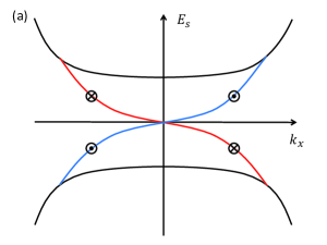
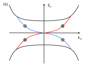
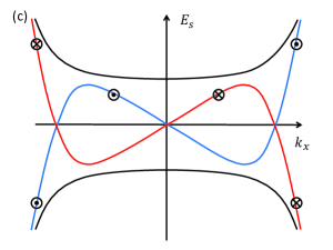
Figure 1: Schematic dispersions for surface bound states in the $A_{1u}$ phase. (a): Single-band or full two-band picture, ${\rm sgn}(mv_{z})>0$, (b): Single-band picture, ${\rm sgn}(mv_{z})<0$, (c): full two-band picture, ${\rm sgn}(mv_{z})<0$. Here, the arrow head (tail) indicates that the spin is pointing out of (in to) the plane. $v<0$.

References

- (1) L. Fu, C. L. Kane and E. J. Mele, Phys. Rev. Lett. 98, 106803 (2007)
- (2) L. Fu and C. L. Kane, Phys. Rev. B 76, 045302 (2007)
- (3) Y. Xia, D. Qian, D. Hsieh, L. Wray, A. Pal, H. Lin, A. Bansil, D. Grauer, Y. S. Hor, R. J. Cava, and M. Z. Hasan, Nature Phys. 5, 398 (2009).
- (4) H. Zhang, C.-X. Liu, X.-L. Qi, X. Dai, Z. Fang and S.-C. Zhang, Nature Physics 5, 438 (2009)
- (5) D. Hsieh, D. Qian, L. Wray, Y. Xia, Y. S. Hor, R. J. Cava and M. Z. Hasan, Nature (London) 452, 970 (2008)
- (6) D. Hsieh, Y. Xia, L. Wray, D. Qian, A. Pal, J. H. Dil, J. Osterwalder, F. Meier, G. Bihlmayer, C. L. Kane, Y. S. Hor, R. J. Cava and M. Z. Hasan, Science 323, 919 (2009)
- (7) Y. L. Chen, J. G. Analytis, J.-H. Chu, Z. K. Liu, S.-K. Mo, X. L. Qi, H. J. Zhang, D. H. Lu, X. Dai, Z. Fang, S. C. Zhang, I. R. Fisher, Z. Hussain, Z.-X. Shen, Science, 325, 178 (2009)
- (8) D. Hsieh, Y. Xia, D. Qian, L. Wray, J. H. Dil, F. Meier, J. Osterwalder, L. Patthey, J. G. Checkelsky, N. P.Ong, A. V. Fedorov, H. Lin, A. Bansil, D. Grauer, Y. S. Hor, R. J. Cava and M. Z. Hasan, Nature 460, 1101 (2009)
- (9) X.-L. Qi, T. L. Hughes, S.-C. Zhang, Phys. Rev. 78, 195424 (2008)
- (10) X.-L. Qi, R. Li, J. Zang and S.-C. Zhang, Science, 323, 1184 (2009)
- (11) Y. S. Hor, A. J. Williams, J. G. Checkelsky, P. Roushan, J. Seo, Q. Xu, H. W. Zandbergen, A. Yazdani, N. P. Ong, and R. J. Cava, Phys. Rev. Lett. 104, 057001 (2010)
- (12) L. A. Wray, S.-Y. Xu, Y. Xia, Y. S. Hor, D. Qian, A. V. Fedorov, H. Lin, A. Bansil, R. J. Cava, and M. Z. Hasan, Nat. Phys. 6, 855 (2010).
- (13) M. Kriener, K. Segawa, Z. Ren, S. Sasaki, and Y. Ando, Phys. Rev. Lett. 106, 127004 (2011)
- (14) Bi2Te3 is also found to be superconducting under pressure JLZhang11 . However, the bulk carriers are holes which are located away from the point, a rather different situation from Cu:Be2Se3. We shall not discuss this compound here any further in this paper.
- (15) J. L. Zhang, S. J. Zhang, H. M. Weng, W. Zhang, L. X. Yang, Q. Q. Liu, S. M. Feng, X. C. Wang, R. C. Yu, L. Z. Cao, L. Wang, W. G. Yang, H. Z. Liu, W. Y. Zhao, S. c. Zhang, X. Dai, Z. Fang and C. Q. Jin, Proc. Acad. Sci. U. S. A. 108, 24 (2011)
- (16) S. Sasaki, M. Kriener, K. Segawa, K. Yada, Y. Tanaka, M. Sato, and Y. Ando, Phys. Rev. Lett. 107, 217001 (2011).
- (17) T. Kirzhner, E. Lahoud, K. Chaska, Z. Salman, and A. Kanigel, B86, 064517 (2012)
- (18) T. V. Bay, T. Naka, Y. K. Huang, H. Luigjes, M. S. Golden, and A. de Visser Phys. Rev. Lett. 108, 057001 (2012)
- (19) N. Levy, T. Zhang, J. Ha, Fred Sharifi, A. A. Talin, Y. Kuk and J. A. Stroscio, arXiv:1211.0267
- (20) L. Fu and E. Berg, Phys. Rev. Lett. 105, 097001 (2010)
- (21) L. Hao and T. K. Lee, Phys. Rev. B 83, 134516 (2011)
- (22) T. H. Hsieh and L. Fu, Phys. Rev. Lett. 108, 107005 (2012).
- (23) A. Yamakage, K. Yada, M. Sato and Y. Tanaka, Phys. Rev. B 85 180509(R) (2012)
- (24) P. W. Anderson, Phys. Rev. B 30, 1549 (1984)
- (25) G. E. Volovik and L. P. Gorkov, Pis’ma Zh. Eksp. Teor. Fiz. 39, 550 (1984) [JETP Lett. 39, 12 (1984)]; Zh. Eksp. Teor. Fiz. 88, 1412 (1985) [Sov. Phys JETP 61, 843 (1985)].
- (26) K. Ueda and T. M. Rice, Phys. Rev. B 31, 7114 (1985).
- (27) E. I. Blount, Phys. Rev. B 32, 2935 (1985).
- (28) M. Sigrist and K. Ueda, Rev. Mod. Phys. 63, 239 (1991)
- (29) S. Yip and A. Garg, Phys. Rev. B 48, 3304 (1993)
- (30) Robert Joynt and Louis Taillefer, Rev. Mod. Phys. 74, 235 (2002)
- (31) Different models have also been employed in the literature, e.g., HZ09 ; Hao11 ; Sasaki11 , hence some modifications must be taken to compare those results with here. In Model I of Hao11 , the spin part in eq (1) was instead written as . Hence all the spins in Hao11 must be rotated by about z in order to compare with ours here. Fortunately, this would not alter anything for pairings between opposite spins, that is, for the , and phases in Table 1. For the two-dimensional odd parity state which involves pairing between parallel spins, this rotation brings in the factors for and respectively, thus interchanges the two entries under in Table 1. We shall not try to provide the comparison with other models in this paper.
- (32) C.-X. Liu, X.-L. Qi, H. J. Zhang, X. Dai, Z. Fang and S.-C. Zhang, Phys. Rev. B 82, 045122 (2010)
- (33) F. Zhang, C. L. Kane and E. J. Mele, Phys. Rev. B 86, 081303 (2012)
- (34) We are using this term with a different meaning from the usual ”two-band superconductivity” in the literature. Here, we only have one Fermi surface for the corresponding normal phase in the absence of pairing potentials.
- (35) A. J. Leggett, Rev. Mod. Phys. 47, 331 (1975)
- (36) There are no entries listed under columns (iii), (iv) and (v) for and , since they do not arise if we insist that there is no momentum dependence when the pairs are expressed in the orbital and spin basis. They can however occur if we allow more general momentum dependence.
- (37) One is free to work in other basis, e.g. Michaeli12 , but the physical picture needed would be different. Also, one would not be able to employ the tables in VG84 ; Ueda85 ; Blount85 ; Sigrist91 ; Yip93 ; Joynt02 .
- (38) K. Michaeli and L. Fu, Phys. Rev. Lett. 109, 187003 (2012)
- (39) We shall not worry about how we define states at . We can define these by approprate limiting procedures. This can lead to discontinuities of these wavefunctions as functions of (see Blount85 ) , but these complications would not occur for the pair wavefunctions, our major concern in this paper.
- (40) The pseudospin obeys under parity while under time-reversal. This is applicable to both and defined below due to eq (2) and (3).
- (41) We are using here for these matrices in primed basis since they do not have the rotational properties of .
- (42) R. Balian and N. R. Werthamer, Phys. Rev. 131, 1553 (1963)
- (43) N. P. Butch, P. Syers, K. Kirshenbaum, A. P. Hope and J. Paglione, Phys. Rev. B 84, 220504(R) (2011)
- (44) A. P. Schnyder, S. Ryu, A. Furusaki, and A. W. W. Ludwig, Phys. Rev. B 78, 195125 (2008).
- (45) M. Sato, Phys. Rev. B 79, 214526 (2009)
- (46) X.-L. Qi, T. L. Hughes, S.-C. Zhang, Phys. Rev. 81, 134508 (2010)
- (47) S.-K. Yip J. Low Temp. Phys. 160, 12 (2010)
- (48) We can separate the reflection due to the vaccum-sample surface and the Andreev reflection due to the order parameter variations by imagining inserting a thin normal layer near the surface, as done in, e.g. Beenakker . Since the reflection coefficient for the hole is given by the complex conjugate of that of the particle, the phase shift from the reflection coefficient of Sec III cancels, if we ignore the small wavevector difference between the particle and hole.
- (49) C. W. J. Beenakker, Phys. Rev. B 46, 12841 (1992)
- (50) These results can be derived easily from solving the Andreev equation, or locating the poles of the Green’s function in, e.g., KO .
- (51) I. O. Kulik and A. N. Omelyanchuk, Sov. J. Low Temp. 3, 459 (1977)
- (52) This sign change arises from , when one derives the Andreev equation.
- (53) There seem to have an ambiguity in the sign of since one can characterize the same phase with antiparallel to by making use of a gauge transformation.